Vectorization of the density matrix and quantum simulation of the von Neumann equation of time-dependent Hamiltonians.

Abstract

Based oh the properties of Lie algebras, in this work we develop a general framework to linearize the von-Neumann equation rendering it in a suitable form for quantum simulations. We show that one of these linearizations of the von-Neumann equation corresponds to the standard case in which the state vector becomes the column stacked elements of the density matrix and the Hamiltonian superoperator takes the form $I\otimes H-H^{\top}\otimes I$ where $I$ is the identity matrix and $H$ is the standard Hamiltonian. It is proven that this particular form belongs to a wider class of ways of linearizing the von Neumann equation that can be categorized by the algebra from which they originated. Particular attention is payed to Hermitian algebras that yield real density matrix coefficients substantially simplifying the quantum tomography of the state vector. Based on this ideas, a quantum algorithm to simulate the dynamics of the density matrix is proposed. It is shown that this method, along with the unique properties of the algebra formed by Pauli strings allows to avoid the use of Trotterization hence considerably reducing the circuit depth. Even though we have used the special case of the algebra formed by the Pauli strings, the algorithm can be readily adapted to other algebras. The algorithm is demonstrated for two toy Hamiltonians using the IBM noisy quantum circuit simulator.

I Introduction

One of the most important applications of quantum computers is the simulation of large quantum systems that are intractable using conventional classical computers Feynman (1982); Lloyd (1996); Nielsen and Chuang (2002). A vast number of quantum techniques to simulate quantum dynamics has been developed with this purpose in mind Georgescu et al. (2014); Miessen et al. (2023). Specially many body systems give rise to extremely large Hamiltonians Abrams and Lloyd (1997) that are classically impossible to tackle even for a small number of particles.

A very common quantum simulation problem is the digital quantum simulation (DQS) of a closed quantum system Lloyd (1996); Abrams and Lloyd (1997); Lidar and Biham (1997); Zalka (1998); Ortiz et al. (2001); Marzuoli and Rasetti (2002); Somma et al. (2002); Verstraete et al. (2009); Berry et al. (2007); Raeisi et al. (2012); Georgescu et al. (2014) which consists in solving the time-dependent Schrödinger equation. In general terms, a DQS algorithm consists of two steps. First the time evolution operator of a given Hamiltonian is expressed as a series of unitary quantum gates through the Jordan-Wigner isomorphism Somma et al. (2002), for example. Second, the time evolution operator is used to propagate an initial state Lloyd (1996); Miessen et al. (2023), typically by shifting locally the wave function forward in time over discrete and sufficiently small time slices Lloyd (1996); Georgescu et al. (2014); Miessen et al. (2023). The Hamiltonian is written as the sum over many simpler interactions $H=\sum_{i=1}^{m}H_{i}$ and the evolution operator can be approximated by $\mathcal{U}(t)=\mathrm{e}^{-iH_{1}\Delta t/\hbar}\mathrm{e}^{-iH_{2}\Delta t/\hbar}\dots\mathrm{e}^{-iH_{m}\Delta t/\hbar}$ as long as the interval $\Delta t$ is small enough. Through the Trotter-Suzuki formula Trotter (1958); Suzuki (1992); Somma (2016), that takes into account the non-commutativity of the $H_{i}$’s, the accuracy of $U(t)$ can then be improved but at the cost of increasing the circuit depth.

Nearly all realistic quantum systems are open systems whose evolution is non-unitary due to the decoherence induced by the unavoidable interaction with the environment. This presents a major difficulty for digital quantum computers that can only operate with a set of unitary gates. This obstacle has spawned a wide range of solutions for the quantum simulation of open quantum systems Tseng et al. (2000); Di Candia et al. (2015); Wang et al. (2011); Wei et al. (2016); Motta et al. (2020); Hu et al. (2020); Kamakari et al. (2022). The following are some examples. The open-system nature of a two-spin NMR ensemble has been employed to simulate the decoherence in a quantum simulation Tseng et al. (2000). Also, a set of ancilla qubits that are designed to have the same effect as the simulated environment have been used to represent the decoherence of an open quantum system Wang et al. (2011). Quantum algorithms have been developed specifically for duality quantum computers that can perform non-unitary operations Wei et al. (2016). More recently, eigenstate and thermal state quantum simulations have been demonstrated employing the quantum analogues of imaginary time evolution and Lanczos algorithms Motta et al. (2020). Of direct relevance to this work is a new kind of open-quantum system simulation algorithm that solves the Lindblad master equation and that has successfully been tested in real digital quantum hardware Kamakari et al. (2022). The algorithm mainly relies on the Kraus matrix representations Kraus (1971); Havel (2003); Nakazato et al. (2006) and an adaptation of the imaginary time evolution algorithm Motta et al. (2020). In general, the Lindblad equation is first vectorized in the form of a Scrhödinger equation through the Kraus operator sum Kraus (1971); Havel (2003); Nakazato et al. (2006); Ramusat and Savona (2021) and then, the anti-Hermitian component of the Hamiltonian is treated through quantum imaginary evolution. The elements of the vectorized density matrix are finally obtained by quantum tomography. The unitary evolution of the Hermitian component of the Hamiltonian is calculated by the standard techniques of DQS listed above.

In this work we are primarily interested in the linearization of the density matrix that is governed by the von Neumann equation

$$i\hbar\frac{d}{dt}\rho(t)=\left[H(t),\rho(t)\right],$$ (1)

where $H$ and $\rho(t)$ are the $N\times N$ matrices for the Hamiltonian and the density matrix. The linearization is typically done by expressing the density matrix using the Kraus operator sum and column stacking the density matrix elements. As we show below, this procedure yields the following linearized von Neumann equation Havel (2003); Kamakari et al. (2022)

$$i\hbar\frac{d}{dt}\left|\boldsymbol{\rho}\right\rangle=\left[I\otimes H(t)-H^{\top}(t)\otimes I\right]\left|\boldsymbol{\rho}\right\rangle,$$ (2)

where $I$ is the $N\times N$ identity matrix and $\left|\boldsymbol{\rho}\right\rangle$ denotes the vector resulting from stacking the columns of $\rho(t)$ from left to right.

We develop a method that generalizes the vectorization process of the von Neumann equation expanding the density matrix in terms of the elements of a Lie algebra. Moreover, we show that the column-stacked density matrix in Eq. (2) is in fact one of the many possible ways of representing $\rho(t)$ as a vector using the elements of a very specific Lie algebra. Instead of using this algebra, whose elements are non Hermitian, we propose expanding the von Neumann equation in terms of Hermitian matrices. The advantage is that the thus vectorized density matrix has purely real coefficients that greatly simplify the quantum tomography of $\left|\boldsymbol{\rho}\right\rangle$. We present the special case of the algebra formed by Pauli strings and with it, implement an algorithm that solves the von Neumann equation to illustrate the method. The method, together with the special properties of Pauli strings, allows to avoid the use of Trotterization therefore reducing the circuit depth. The algorithm was tested for the von Neumann equation of the magnetic resonance Hamiltonian using Qiskit in the noisy quantum circuit simulator qasm_simulator IBM . The code can be downloaded from Kunold .

II Vectorization of the density matrix.

Any $N\times N$ square matrix $W$ can be expressed as the linear combination of the elements of the finite Lie algebra $\mathfrak{g}_{n}=\left\{g_{1},g_{2},\dots,g_{n}\right\}$, as

$$W=\sum_{i=1}^{n}w_{i}g_{i}=\boldsymbol{g}^{\top}\boldsymbol{w}$$ (3)

where $\boldsymbol{g}^{\top}=\left(g_{1},g_{2},\dots,g_{n}\right)$, $\boldsymbol{w}^{\top}=\left(w_{1},w_{2},\dots,w_{n}\right)$, $g_{i}\in\mathbb{C}^{N\times N}$ and $w_{i}\in\mathbb{C}$. If $W$ is known, the coefficients $w_{i}$ can be calculated as

$$w_{i}=\frac{1}{\mathrm{Tr}\left[g^{\dagger}_{i}g_{i}\right]}\mathrm{Tr}\left[g^{\dagger}_{i}W\right],$$ (4)

provided that the elements of the algebra are orthogonal under the Frobenius inner product, namely

$$\mathrm{Tr}\left[g_{i}^{\dagger}g_{j}\right]=\mathrm{Tr}\left[g^{\dagger}_{i}g_{i}\right]\delta_{i,j}.$$ (5)

Not all algebras have orthogonal elements, however, one can always find a linear combination of them that does meet (5). Such combinations might be generated, for example, through the Gram-Schmidt method.

One of the fundamental properties of Lie algebras is that their elements form a closed commutator algebra described by

$$\left[g_{i},g_{j}\right]=i\hbar\sum_{k}c_{i,j,k}g_{k}.$$ (6)

where the Lie bracket of $\mathfrak{g}_{n}$ has been chosen to be the commutator $\left[g_{i},g_{j}\right]=g_{i}g_{j}-g_{j}g_{i}$. From this definition it is straight forward to show that the structure constants $c_{i,j,k}$ have the property

$$c_{i,j,k}=-c_{j,i,k}.$$ (7)

The explicit form of the structure constants

$$c_{i,j,k}=\frac{\mathrm{Tr}\left[g^{\dagger}_{k}\left[g_{i},g_{j}\right]\right]}{{i\hbar}\Tr[g_{k}^{\dagger}g_{k}]}=\frac{\mathrm{Tr}\left[\left[g_{i},g_{j}\right]g^{\dagger}_{k}\right]}{{i\hbar}\Tr[g_{k}^{\dagger}g_{k}]}$$ (8)

is obtained by combining Eqs. (5) and (6). In the case of an algebra $\mathfrak{h}_{n}=\left\{h_{1},h_{2},\dots,h_{n}\right\}$ formed only by Hermitian matrices the structure constants acquire a new and useful property, the invariance with respect to cyclic permutation of the indices

$$c_{i,j,k}=\frac{\mathrm{Tr}\left[\left[h_{i},h_{j}\right]h_{k}\right]}{i\hbar\mathrm{Tr}\left[h_{k}h_{k}\right]}=\frac{\mathrm{Tr}\left[h_{i}h_{j}h_{k}-h_{j}h_{i}h_{k}\right]}{i\hbar\mathrm{Tr}\left[h_{k}h_{k}\right]}\\ =\frac{\mathrm{Tr}\left[h_{k}h_{i}h_{j}-h_{i}h_{k}h_{j}\right]}{i\hbar\mathrm{Tr}\left[h_{k}h_{k}\right]}=\frac{\mathrm{Tr}\left[\left[h_{k},h_{i}\right]h_{j}\right]}{i\hbar\mathrm{Tr}\left[h_{i}h_{i}\right]}=c_{k,i,j},$$ (9)

as long as $\mathrm{Tr}\left[h_{i}h_{i}\right]=\mathrm{Tr}\left[h_{k}h_{k}\right]$. Note that the properties (8) and (9) imply that $c_{i,j,k}$ is fully antisymmetric.

With these definitions at hand we can proceed to vectorize the von Neumann equation. In terms of the most general algebra $\mathfrak{g}_{n}$ the density matrix can be expanded as

$$\rho(t)=\sum_{i}g_{i}\rho_{i}(t)=\boldsymbol{g}^{\top}\boldsymbol{\rho}(t),$$ (10)

where $\boldsymbol{\rho}(t)=(\rho_{1}(t),\rho_{2}(t),\dots,\rho_{n}(t))$ and from Eq. (4) the coefficients are

$$\rho_{i}(t)=\frac{1}{\Tr\left[g_{i}^{\dagger}g_{i}\right]}\left[g_{i}^{\dagger}\rho(t)\right].$$ (11)

Multiplying the left and right-hand side terms of (1) by $g_{k}^{\dagger}$ and tracing it follows that

$$i\hbar\frac{d}{dt}\Tr\left[g_{k}^{\dagger}\rho(t)\right]=\sum_{j}\Tr\left[g_{k}^{\dagger}\left[H(t),g_{j}\right]\right]\Tr[g^{\dagger}_{j}\rho(t)]\\ =\sum_{i,j}\Tr[g^{\dagger}_{i}g_{i}]a_{i}(t)\Tr\left[g_{k}^{\dagger}\left[g_{i},g_{j}\right]\right]\Tr[g^{\dagger}_{j}\rho(t)]\\ =i\hbar\sum_{i,j}\Tr[g^{\dagger}_{k}g_{k}]\Tr[g^{\dagger}_{i}g_{i}]c_{i,j,k}a_{i}(t)\Tr[g^{\dagger}_{j}\rho(t)].$$ (12)

Because of (3) and (4), the Hamiltonian can be expressed as the decomposition

$$H(t)=\sum_{i}a_{i}(t)g_{i}=\boldsymbol{a}^{\top}(t)\boldsymbol{g}$$ (13)

where

$$a_{i}(t)=\frac{1}{\mathrm{Tr}\left[g_{i}^{\dagger}g_{i}\right]}\mathrm{Tr}\left[g_{i}^{\dagger}H(t)\right],$$ (14)

are the Hamiltonian coefficients and $\boldsymbol{a}^{\top}(t)=(a_{1}(t),a_{2}(t),\dots,a_{n}(t))$. Equation (12) can be put in the more succinct form

$$i\hbar\frac{d}{dt}\boldsymbol{\rho}(t)=\mathcal{H}(t)\boldsymbol{\rho}(t)$$ (15)

where

$$\mathcal{H}(t)=\sum_{i}\mathcal{H}_{i},$$ (16)

is the Hamiltonian superoperator,

$$\mathcal{H}_{i}=i\hbar\Tr[g^{\dagger}_{k}g_{k}]\Tr[g^{\dagger}_{i}g_{i}]C_{i}a_{i}(t),$$ (17)

and $C_{i}$ is the matrix whose elements are the structure constants $(C_{i})_{j,k}=c_{i,j,k}$. Equation (15) is a general form of the vectorized von Neumann equation.

At this point it is natural to ask what is the connection between this version of the von Neumann equation and (2). To address this question we introduce two auxiliary algebras. First consider the algebra $\mathfrak{q}_{n}=\left\{q_{1},q_{2},\dots,q_{n}\right\}$ formed by the $N\times N$ sparse matrices $q_{i}$ that only have a $1$ that progressively shifts from top to bottom and from left to right as $i$ goes from $1$ to $n=N^{2}$. More explicitly $(q_{i})_{j,k}=\delta_{j,i_{1}}\delta_{k,i_{2}}$ where

$$i_{1} = (i-1)\bmod N+1,$$ (18)

$$i_{2} = [(i-1)/N]+1.$$ (19)

Therefore, the vector of dimension $n=N^{2}$ formed by the coefficients of a given $N\times N$ matrix in terms of $\mathfrak{q}_{n}$ corresponds to the stacked columns thereof. Indeed, the vector formed by the coefficients of $W$ in terms of $\mathfrak{q}_{n}$ are the matrix elements of $W$

$$w_{i}=\frac{\Tr[q_{i}^{\dagger}W]}{\Tr[q_{i}^{\dagger}q_{i}]}=\Tr[q_{i}^{\dagger}W]=(W)_{i_{1},i_{2}}$$ (20)

where $i_{1}$ and $i_{2}$ are given by (18) and (19), respectively.

The second auxiliary algebra is $\mathfrak{q}_{n}^{\otimes 2}$ $=\mathfrak{q}_{n}\otimes\mathfrak{q}_{n}$ $=\{q_{1}\otimes q_{1},$ $q_{1}\otimes q_{2},$ $\dots,q_{n-1}\otimes q_{n},$ $q_{n}\otimes q_{n}\}$ $=\{Q_{1,1},$ $Q_{1,2},$ $\dots,Q_{n,n-1},$ $Q_{n,n}\}$ where $Q_{i,j}$ is an $N^{2}\times N^{2}$ sparse matrix that has a $1$ in the $i,j$ position. It is important to note that even though in general $Q_{i,j}\neq q_{i}\otimes q_{j}$, it is possible to establish a one to one relation

$$Q_{k,l}=q_{b}\otimes q_{a}$$ (21)

for

$$a = N\left[\left(k-1\right)\bmod N\right]+\left(l-1\right)\bmod N+1,$$ (22)

$$b = N\left[\left(k-1\right)/N\right]+\left[\left(l-1\right)/N\right]+1.$$ (23)

Following a similar procedure as in Eq. (12) the expansion of the von Neumann equation in the $\mathfrak{q}_{n}$ altakes the form

$$i\hbar\frac{d}{dt}\Tr\left[q_{k}^{\dagger}\rho(t)\right]=\sum_{j}\Tr\left[q_{k}^{\dagger}\left[H(t),q_{j}\right]\right]\Tr[q^{\dagger}_{j}\rho(t)]\\ =\sum_{j}\Tr\left[q_{k}^{\dagger}H(t)q_{j}I-q_{k}^{\dagger}Iq_{j}H(t)\right]\Tr[q^{\dagger}_{j}\rho(t)].$$ (24)

In Appendix A it is shown that if $A$ and $B$ are two $N\times N$ matrices then

$$\Tr\left[q_{i}^{\dagger}Aq_{j}B\right]=\Tr\left[Q_{i,j}^{\dagger}B^{\top}\otimes A\right]=(B^{\top}\otimes A)_{i,j}.$$ (25)

With this, Eq. (24) becomes

$$i\hbar\frac{d}{dt}\Tr\left[q_{k}^{\dagger}\rho(t)\right]\\ =\sum_{j}\bigg{(}I\otimes H(t)-H^{\top}(t)\otimes I\bigg{)}_{k,j}\Tr\left[q_{j}^{\dagger}\rho(t)\right],$$ (26)

that, in full consistency with Eq. (2), can also be written as the vectorial expression

$$i\hbar\frac{d}{dt}\boldsymbol{\rho}(t)=\sum_{j}\bigg{(}I\otimes H(t)-H^{\top}(t)\otimes I\bigg{)}\boldsymbol{\rho}(t).$$ (27)

Hence, the von Neumann equation that stems from the Kraus sum is a particular case of (15) when it is expanded in terms of the algebra $\mathfrak{q}_{n}$. In this case $\boldsymbol{\rho}(t)$ corresponds to the stacked columns of the density matrix. The entries of the vector $\boldsymbol{\rho}(t)$ are, however, complex numbers since $\mathfrak{q}_{n}$ is comprised of non-Hermitian matrices. This substantially complicates the quantum tomography of $\boldsymbol{\rho}(t)$ whose elements may have non-vanishing phases.

To circumvent this difficulty one can use any Hermitian algebra $\mathfrak{h}_{n}$ that yields real entries for $\boldsymbol{\rho}(t)$. In this base, the Hamiltonian and the density matrix

$$H(t)=\sum_{i}a_{i}(t)h_{i}=\boldsymbol{a}^{\top}(t)\boldsymbol{h},$$ (28)

$$\rho(t)=\sum_{i=1}^{n}h_{i}\rho_{i}(t)=\boldsymbol{h}^{\top}\boldsymbol{\rho}(t)$$ (29)

are expressed as the linear combination of the elements of the finite Lie algebra $\mathfrak{h}_{n}=\left\{h_{1},h_{2},\dots,h_{n}\right\}$ with $\boldsymbol{h}^{\top}=(h_{1},h_{2},\dots,h_{n})$ and $n=2^{N}$. The Hamiltonian coefficients

$$a_{i}(t)=\frac{1}{\mathrm{Tr}\left[h_{i}h_{i}\right]}\mathrm{Tr}\left[Hh_{i}\right].$$ (30)

are real and, in general, time-dependent. Similarly, the density matrix coefficients are

$$\rho_{i}(t)=\frac{1}{\mathrm{Tr}\left[h_{i}h_{i}\right]}\mathrm{Tr}\left[\rho(t)h_{i}\right].$$ (31)

As before, $\boldsymbol{a}(t)=(a_{1}(t),a_{2}(t),\dots,a_{n}(t))$ and $\boldsymbol{\rho}(t)=(\rho_{1}(t),\rho_{2}(t),\dots,\rho_{n}(t))$. From (16) the Hamiltonian superoperator is given by

$$\mathcal{H}(t)=\sum_{i}\mathcal{H}_{i}(t)$$ (32)

where

$$\mathcal{H}_{i}(t)=i\hbar\Tr[h_{k}h_{k}]\Tr[h_{i}h_{i}]C_{i}a_{i}(t).$$ (33)

Note that $\mathcal{H}$ is Hermitian because the coefficients $a_{i}(t)$ are real and the structure constants are fully antisymmetric, i.e.,

$$c_{i,j,k}=-c_{i,k,j},$$ (34)

and therefore $C_{k}=-C_{k}^{\top}$ is skew-symmetric.

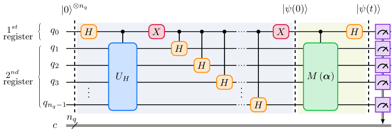
Figure 1: Main quantum algorithm to determine the dynamics of the density matrix coefficients $\rho_{1}(t)$,$\dots$, $\rho_{n}(t)$. (b) Controlled $M\left(\boldsymbol{\alpha}\right)$ gate expressed as a sequence of differential time steps. (c) One time step controlled differential $M\left(d\boldsymbol{\alpha}\right)$ gate expressed as the series of Hamiltonian gates generated by the structure constants of the Pauli strings.

III Time evolution

At first glance it would seem reasonable to find the evolution operator by directly applying the standard techniques of DQS to (15). However, to do so efficiently, it would be convenient to leverage the structure and the symmetries of the linear operator $\mathcal{H}$ in (16). These are not obvious from the expression of $\mathcal{H}$. But the contraction $C_{i}a_{i}(t)$ ($i=1,2,\dots,n$) signals the fact that only the $n$ structure constants are needed to generate the time evolution Somma (2016) and not $n^{2}=n\times n$ as the dimension of $\mathcal{H}$ would suggest. Instead of following this line of reasoning we resort to the Lie algebraic method to prove that indeed only $n$ elements are needed to generate the time evolution.

The Lie algebraic method enables the exact determination of evolution operators for time-dependent Hamiltonians of finite dimension or having a dynamical algebra. Though the general method is thoroughly discussed in Sandoval-Santana et al. (2019) a quick review is provided here for completeness.

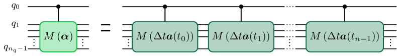
Figure 2: Controlled $M\left(\boldsymbol{\alpha}\right)$ gate expressed as a sequence of differential time steps.

One possible way of expressing the evolution operator of the Hamiltonian (28) is $\mathcal{U}(t)=U^{\dagger}(t)=U_{1}^{\dagger}(t)U_{2}^{\dagger}(t)\dots U_{n}^{\dagger}(t)$ where

$$U_{k}(t)=\exp\left[\frac{i}{\hbar}\alpha_{k}(t)h_{k}\right],$$ (35)

is the unitary transformation generated by the $k$-th element of $\mathfrak{h}_{n}$. Each $U_{k}$ transforms $\boldsymbol{h}$ according to

$$U_{k}(t)\boldsymbol{h}U_{k}^{\dagger}(t)=M_{k}\left(\alpha_{k}(t)\right)\boldsymbol{h},$$ (36)

where the explicit form of the matrices $M_{k}\left(\alpha_{k}(t)\right)$ is given by

$$M_{k}(\alpha_{k}(t))=\exp\left[-\alpha_{k}(t)C_{k}\right].$$ (37)

The matrices $M_{k}(\alpha_{k}(t))$ are unitary since, as mentioned earlier, $C_{k}=-C_{k}^{\top}$ is skew-symmetric in accordance with (34). Therefore, by performing a time evolution over $\boldsymbol{h}$ we obtain

$$U(t)\boldsymbol{h}U^{\dagger}(t)=M(\boldsymbol{\alpha}(t))\boldsymbol{h},$$ (38)

where

$$M(\boldsymbol{\alpha}(t))=M_{1}(\alpha_{1}(t))M_{2}(\alpha_{2}(t))\dots M_{n}(\alpha_{n}(t)).$$ (39)

The explicit time-dependence of the $\alpha_{k}(t)$ parameters is yet unknown but can be derived from the Schrödinger equation

$$\big{(}H(t)-p_{t}\big{)}\left|\psi(t)\right\rangle=0,$$ (40)

where $p_{t}=i\hbar\partial/\partial t$ is the energy operator. The Hamiltonian and the energy operator transform according to

$$U(t)HU^{\dagger}(t) = \boldsymbol{a}^{\top}M_{1}M_{2}\dots M_{n}\boldsymbol{h}=\boldsymbol{a}^{\top}M\boldsymbol{h},$$ (41)

$$U(t)p_{t}U(t)^{\dagger} = p_{t}+\dot{\boldsymbol{\alpha}}^{\top}V^{\top}\boldsymbol{h}$$ (42)

where

$$V^{\top} = I_{1}M_{2}(\alpha_{2})\dots M_{n}(\alpha_{n})$$ (43)

$$+ I_{2}M_{3}(\alpha_{3})\dots M_{n}(\alpha_{n})+\dots+I_{n},$$

$$(I_{k})_{ij} = \delta_{i,k}\delta_{j,k}.$$ (44)

It then follows from Eqs. (41) and (42) that the Schrödinger equation under $U(t)$ becomes

$$U(t)\left(H-p_{t}\right)U^{\dagger}(t)U(t)\left|\psi(t)\right\rangle\\ =\left[\boldsymbol{a}^{\top}M\boldsymbol{h}-\dot{\boldsymbol{\alpha}}^{\top}V^{\top}\boldsymbol{h}-p_{t}\right]U(t)\left|\psi(t)\right\rangle=0.$$ (45)

Making

$$\boldsymbol{a}^{\top}(t)M\left(\boldsymbol{\alpha}(t)\right)\boldsymbol{h}-\dot{\boldsymbol{\alpha}}(t)^{\top}V^{\top}\left(\boldsymbol{\alpha}(t)\right)\boldsymbol{h}=0,$$ (46)

or, equivalently

$$\dot{\boldsymbol{\alpha}}(t)=\boldsymbol{F}\left(t,\boldsymbol{\alpha}(t)\right)=V^{-1}\left(\boldsymbol{\alpha}(t)\right)M^{\top}\left(\boldsymbol{\alpha}(t)\right)\boldsymbol{a}(t),$$ (47)

we arrive at the result that $p_{t}U(t)\left|\psi(t)\right\rangle=0$. Since $p_{t}=i\hbar\partial/\partial t$, the previous equation will only hold if $\mathcal{U}(t)=U^{\dagger}(t)$ and $U(t)\left|\psi(t)\right\rangle=\left|\psi_{0}\right\rangle=\left|\psi(0)\right\rangle$ is the initial state. Equation (47) consists of a system of $n$ ordinary differential equations for $\alpha_{1}(t),\alpha_{2}(t)$, $\dots\alpha_{n}(t)$. The explicit time dependence of the $\boldsymbol{\alpha}(t)$ parameters comes from the solution of (47) along with the initial condition

$$\boldsymbol{\alpha}(0)=0,$$ (48)

necessary to ensure that $U(0)=\mathcal{U}(0)=1$.

As we mentioned above, since both $\rho(t)$ and $\boldsymbol{h}$ are Hermitian matrices, the elements of $\boldsymbol{\rho}$ are real. This crucial feature significantly simplify the quantum tomography of the density matrix coefficients allowing to easily determine its elements through phase kickback Cleve et al. (1998) with only one auxiliary qbit. Using Eqs. (38) and (29) the evolution of the density matrix operator in the Schrödinger picture is expressed according to

$$\rho(t)=\mathcal{U}(t)\rho(0)\mathcal{U}^{\dagger}(t)=U^{\dagger}(t)\rho(0)U(t)\\ =\sum_{i}U^{\dagger}(t)h_{i}U(t)\rho_{i}(0)=U^{\dagger}(t)\boldsymbol{h}^{\top}U(t)\boldsymbol{\rho}(0)\\ =\boldsymbol{h}^{\top}(0)M(\boldsymbol{\alpha}(t))\boldsymbol{\rho}(0).$$ (49)

From the comparison of this result with Eq. (29) it follows that the time-dependent density matrix may be cast in the shape of a vector as

$$\boldsymbol{\rho}(t)=M(\boldsymbol{\alpha}(t))\boldsymbol{\rho}(0).$$ (50)

Except for a normalization constant, notice that $M^{\top}(\boldsymbol{\alpha}(t))$ is associated to the superoperator of $U^{\dagger}(t)$ acting on the vectorized density matrix $\boldsymbol{\rho}(t)$ in the Fock-Liouville space generated by $\mathfrak{h}_{n}$. In other words, the evolution of the density matrix thus maps onto the evolution of a quantum state vector

$$\left|\boldsymbol{\rho}(t)\right\rangle=M(\boldsymbol{\alpha}(t))\left|\boldsymbol{\rho}(0)\right\rangle,$$ (51)

where $M(\boldsymbol{\alpha}(t))$ is a super-evolution operator. The density matrix can be expanded as

$$\left|\boldsymbol{\rho}(t)\right\rangle=\sum_{i}\rho_{i}(t)\left|h_{i}\right\rangle,$$ (52)

where $\rho_{i}(t)$ are the normalized density matrix coefficients ($\sum_{i}\rho_{i}^{2}(t)=1$) and there is a one-to-one relation between the Fock-Liouville states $\left|h_{i}\right\rangle$ and the matrices $h_{i}$.

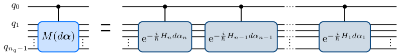
Figure 3: One time step controlled differential $M\left(d\boldsymbol{\alpha}\right)$ gate expressed as the series of Hamiltonian gates generated by the structure constants of the Pauli strings.

Equation (50) proves that the time evolution of the vectorized density matrix is generated by only $n$ elements that correspond to the structure constants $C_{k}$ as was hinted at the beginning of this section.

IV Algorithm

We now provide a quantum simulation algorithm for the density matrix $\rho(t)$ obeying the von-Neumann equation (1) expanded in a general algebra $\mathfrak{h}_{n}$. It illustrates the time evolution and the quantum tomography of the density matrix.

Equation (50) is the underpinning element of the algorithm. It allows for the computation of $\rho(t)$ through a series of time steps $t_{m}$ of step size $\Delta t=t_{m}-t_{m-1}$ as

$$\left|\boldsymbol{\rho}(t_{m})\right\rangle=M(d\boldsymbol{\alpha}_{m})M(d\boldsymbol{\alpha}_{m-1})\dots M(d\boldsymbol{\alpha}_{1})\left|\boldsymbol{\rho}(0)\right\rangle,$$ (53)

where, from (47)

$$d\boldsymbol{\alpha}_{m}=\boldsymbol{\alpha}(t_{m})-\boldsymbol{\alpha}(t_{m-1})=\frac{\dot{\boldsymbol{\alpha}}(t_{m-1})}{1!}\Delta t\\ +\frac{\ddot{\boldsymbol{\alpha}}(t_{m-1})}{2!}\Delta t^{2}+\dots=\boldsymbol{F}\left(t_{m-1},\boldsymbol{\alpha}(t_{m-1})\right)\frac{\Delta t}{1!}\\ +\dot{\boldsymbol{F}}\left(t_{m-1},\boldsymbol{\alpha}(t_{m-1})\right)\frac{\Delta t^{2}}{2!}+\dots\,\,.$$ (54)

Each time step in (54) can be regarded as an independent differential time evolution so that, from the initial condition (48), we can make $\boldsymbol{\alpha}(t_{m-1})=0$ without any loss of generality. Because of this, $V^{-1}\left(\boldsymbol{\alpha}(t_{m-1})\right)=V^{-1}\left(0\right)=I$ and $M^{\top}\left(\boldsymbol{\alpha}(t_{m-1})\right)=M^{\top}\left(0\right)=I$ and consequently the first order term in Eq. (54) gives

$$\boldsymbol{F}\left(t_{m-1},\boldsymbol{\alpha}(t_{m-1})\right)\frac{\Delta t}{1!}\\ =V^{-1}\left(\boldsymbol{\alpha}(t_{m-1})\right)M^{\top}\left(\boldsymbol{\alpha}(t_{m-1})\right)\boldsymbol{a}(t_{m-1})\Delta t\\ =\boldsymbol{a}(t_{m-1})\Delta t.$$ (55)

The second order term is

$$\dot{\boldsymbol{F}}\left(t_{m-1},\boldsymbol{\alpha}(t_{m-1})\right)\frac{\Delta t^{2}}{2!}=\bigg{[}\dot{V}^{-1}\left(\boldsymbol{\alpha}(t)\right)M^{\top}\left(\boldsymbol{\alpha}(t)\right)\boldsymbol{a}(t)\\ +V^{-1}\left(\boldsymbol{\alpha}(t)\right)\dot{M}^{\top}\left(\boldsymbol{\alpha}(t)\right)\boldsymbol{a}(t)\\ +V^{-1}\left(\boldsymbol{\alpha}(t)\right)M^{\top}\left(\boldsymbol{\alpha}(t)\right)\dot{\boldsymbol{a}}(t)\bigg{]}\frac{\Delta t^{2}}{2!}\\ =\bigg{[}\dot{V}^{-1}\left(\boldsymbol{\alpha}(t)\right)\boldsymbol{a}(t)+\dot{M}^{\top}\left(\boldsymbol{\alpha}(t)\right)\boldsymbol{a}(t)\\ +\dot{\boldsymbol{a}}(t)\bigg{]}\frac{\Delta t^{2}}{2!}.$$ (56)

Using (43), (44) and the identity

$$\dot{V}^{-1}\left(\boldsymbol{\alpha}(t_{m-1})\right)\\ =-V^{-1}\left(\boldsymbol{\alpha}(t_{m-1})\right)\dot{V}\left(\boldsymbol{\alpha}(t_{m-1})\right)V^{-1}\left(\boldsymbol{\alpha}(t_{m-1})\right)\\ =-\dot{V}\left(\boldsymbol{\alpha}(t_{m-1})\right),$$ (57)

the first element of (56) reduces to

$$\bigg{(}\dot{V}^{-1}\left(\boldsymbol{\alpha}(t)\right)\boldsymbol{a}(t)\bigg{)}_{i}=\sum_{k=1}^{n-1}\sum_{j=k+1}^{n}c_{i,j,k}a_{j}(t)a_{k}(t).$$ (58)

The second element of (56) vanishes, i.e.,

$$\bigg{(}\dot{M}^{\top}\left(\boldsymbol{\alpha}(t)\right)\boldsymbol{a}(t)\bigg{)}_{i}=\sum_{k=1}^{n}\sum_{j=1}^{n}c_{i,j,k}a_{j}(t)a_{k}(t)=0,$$ (59)

because $c_{i,j,k}a_{j}(t)a_{k}(t)$ is fully antisymmetric. Thus, the second order term is given by

$$\dot{F}_{i}\left(t_{m-1},\boldsymbol{\alpha}(t_{m-1})\right)\frac{\Delta t^{2}}{2!}\\ =\Bigg{[}\sum_{k=1}^{n-1}\sum_{j=k+1}^{n}c_{i,j,k}a_{j}(t)a_{k}(t)+\dot{a}_{i}(t)\Bigg{]}\frac{\Delta t^{2}}{2!}.$$ (60)

Gathering all the contributions up to sencond order in $\Delta t$ yields

$$\big{(}d\boldsymbol{\alpha}_{m}\big{)}_{i}=\Delta t\,a_{i}(t_{m-1})+\frac{\Delta t^{2}}{2}\dot{a}_{i}(t_{m-1})\\ +\frac{\Delta t^{2}}{2}\sum_{k=1}^{n-1}\sum_{j=k+1}^{n}c_{i,j,k}a_{j}(t)a_{k}(t)+O(\Delta t^{3}),$$ (61)

where $\big{(}d\boldsymbol{\alpha}_{m}\big{)}_{i}$ is the $i$-th component of $d\boldsymbol{\alpha}_{m}$ with $i=1,2,\dots n$. Equation (47) and consequently (61) take into account the ordering of the Hamiltonian gates prescribed by Eq. (41) hence enabling us to avoid Trotterization provided that we aim to errors of the order of $\Delta t^{3}$.

More accurate approximations of $d\boldsymbol{\alpha}(t_{m})$ could iteratively be built up to a certain tolerated error of $\Delta t$ reducing the number of time steps and quantum gates. However, this would imply a heavy load of operations in the classical stage of the computation that could undermine the effectiveness of the algorithm. Hence, it should be established at what order of $\Delta t$ the costs of calculating $d\boldsymbol{\alpha}_{m}$ outweigh the gain in precision.

V Quantum circuit

The fundamental stages of the quantum circuit are presented in Fig. 1. The Hamiltonian and $M(\boldsymbol{\alpha}(t))$ are considered to have arbitrary dimension $n=2^{n_{q}-1}$ where $n_{q}$ is the number of required qbits to perform the quantum simulation considering that an extra control qbit is needed for the quantum tomography of $\ket{\boldsymbol{\rho}}$. The control qbit and the remaining ones will be termed first and second registers, respectively.

The first stage is the initial state preparation. In it, the goal is to set the initial state to the superposition

$$\left|\psi(0)\right\rangle=\left|0\right\rangle\otimes\big{[}\left|u\right\rangle\big{]}+\left|1\right\rangle\otimes\big{[}\left|\boldsymbol{\rho}(0)\right\rangle\big{]}.$$ (62)

The second part of the previous state initializes the density matrix coefficients to

$$\left|\boldsymbol{\rho}(0)\right\rangle=\sum_{i=1}^{n}\rho_{i}(0)\left|h_{i}\right\rangle$$ (63)

and the first is used as an ancillary uniform superposition

$$\left|u\right\rangle=2^{-n/2}\sum_{i=1}^{n}\left|h_{i}\right\rangle,$$ (64)

later on used to carry out the phase kickback. Conveniently, the density matrix coefficients $\rho_{i}(0)$ are arranged so that the binary string of $i-1$ matches the second register.

The first Hadamard gate ($H$-gate) puts the control qbit in the superposition

$$\left|\psi_{1}\right\rangle=\left(\left|0\right\rangle+\left|1\right\rangle\right)/\sqrt{2}\otimes[\left|0\right\rangle^{\otimes(n_{q}-1)}].$$ (65)

From this point on the part of the state within square braces refers to the second register. The role of the controlled $U_{H}$ gate is to set the initial condition for the normalized components of the density matrix vector $\left|\boldsymbol{\rho}(0)\right\rangle$. This section of the circuit can be represented by the unitary transformation

$$P_{0}\otimes[I]+P_{1}\otimes[U_{H}]$$ (66)

where $P_{0}=\left|0\right\rangle\left\langle 0\right|$ and $P_{1}=\left|1\right\rangle\left\langle 1\right|$ are the standard projectors. The purpose of this gate is to initialize the second register, whose control qbit is $\left|1\right\rangle$, to the normalized coefficients of $\left|\boldsymbol{\rho}(0)\right\rangle$ living the other unmodified. Given that the second register is initially set to $\left|0\right\rangle^{\otimes(n_{q}-1)}$ by default, the first column vector of the $U_{H}$ must be ($\rho_{1}(0),\rho_{2}(0),\dots,\rho_{n}(0))$. There are many variants of the $U_{H}$ matrix that meet this requirement and that of being unitary. One option is the Householder matrix given by

$$U_{H}=I-\frac{\left(\boldsymbol{\rho}-\boldsymbol{u}_{1}\right)\left(\boldsymbol{\rho}-\boldsymbol{u}_{1}\right)^{\top}}{\left(1-\rho_{1}\right)},$$ (67)

where $\boldsymbol{u}_{1}=(1,0,\dots,0)^{\top}$. The singularity produced when $\rho_{1}=1$ and $\rho_{2}=..=\rho_{n}=0$ can be avoided by choosing $\boldsymbol{u}_{2}$,… or $\boldsymbol{u}_{n}$ instead of $\boldsymbol{u}_{1}$. The following controlled $H$-gates set the part of the second register that is proportional to the control qbit $\left|0\right\rangle$ to a uniform superposition. This segment of the circuit can be cast in the form of the transformation

$$X\otimes[I](P_{0}\otimes[I]+P_{1}\otimes[H^{\otimes(n_{q}-1)}])X\otimes[I]\\ =P_{0}\otimes[H^{\otimes(n_{q}-1)}]+P_{1}\otimes[I].$$ (68)

After collecting the gate transformations and from some elementary algebra it follows that the initial state is given by

$$\left|\psi(0)\right\rangle=\left(P_{0}\otimes[H^{\otimes(n_{q}-1)}]+P_{1}\otimes[I]\right)\\ \times\left(P_{0}\otimes[I]+P_{1}\otimes[U_{H}]\right)\left|0\right\rangle^{\otimes n_{q}}\\ =\frac{1}{\sqrt{2}}\left|0\right\rangle\otimes\left[H^{\otimes(n_{q}-1)}\left|0\right\rangle^{\otimes(n_{q}-1)}\right]\\ +\frac{1}{\sqrt{2}}\left|1\right\rangle\otimes\left[U_{H}\left|0\right\rangle^{\otimes(n_{q}-1)}\right]\\ =\frac{\left|0\right\rangle}{\sqrt{2}}\otimes\left[\sum_{i=1}^{n}\frac{1}{2^{n/2}}\left|h_{i}\right\rangle\right]+\frac{\left|1\right\rangle}{\sqrt{2}}\otimes\bigg{[}\sum_{i=1}^{n}\rho_{i}(t)\left|h_{i}\right\rangle\bigg{]}\\ =\frac{1}{\sqrt{2}}\left|0\right\rangle\otimes\big{[}\left|u\right\rangle\big{]}+\frac{1}{\sqrt{2}}\left|1\right\rangle\otimes\big{[}\left|\boldsymbol{\rho}(0)\right\rangle\big{]},$$ (69)

which is consistent with (62).

The next portion of the circuit is devoted to the actual time evolution of $\left|\boldsymbol{\rho}(t)\right\rangle$. The action of the controlled $M(\boldsymbol{\alpha}(t))$ gate on the initial state $\left|\psi(0)\right\rangle$ can be expressed as

$$\left(P_{0}\otimes\left[I\right]+P_{1}\otimes\left[M(\boldsymbol{\alpha})\right]\right)\left|\psi(0)\right\rangle\\ =\frac{\left|0\right\rangle}{\sqrt{2}}\otimes\left[\sum_{i=1}^{n}\frac{1}{2^{n/2}}\left|h_{i}\right\rangle\right]+\frac{\left|1\right\rangle}{\sqrt{2}}\otimes\bigg{[}M(\boldsymbol{\alpha}(t))\left|\boldsymbol{\rho}(0)\right\rangle\bigg{]}\\ =\frac{\left|0\right\rangle}{\sqrt{2}}\otimes\big{[}\left|u\right\rangle\big{]}+\frac{\left|1\right\rangle}{\sqrt{2}}\otimes\big{[}\left|\boldsymbol{\rho}(t)\right\rangle\big{]}.$$ (70)

As it is shown in Fig. 2, the controlled $M(\boldsymbol{\alpha})$ gate is broken down into small time steps according to Eq. (53). In agreement with Eqs. (37) and (39) each differential time step $M(d\boldsymbol{\alpha})$ is decomposed into $n-1$ Hamiltonian gates of the form

$$M_{k}\left(d\alpha_{k}\right)=\exp\left(-\frac{i}{\hbar}H_{k}d\alpha_{k}\right)$$ (71)

where the Hamiltonian operator is connected to the structure constants through

$$H_{k}=-iC_{k},$$ (72)

as can be seen in Fig. 3. These gates can be synthetized for $SU(2^{N})$ operations with arbitrary number of qbits by means of Cartan decomposition Khaneja and Glaser (2001); Vidal and Dawson (2004); Drury and Love (2008); Dağlı et al. (2008), and other alternative methods Berry et al. (2015); Kökcü et al. (2022). Yet, the complexity and depth of the quantum circuits increases exponentially with the number of qbits producing fast fidelity decays. Fortunately, the structure constants $C_{k}$ acquire properties that facilitate the implementation of the Hamiltonian gates if we restrict ourselves to the algebra $\mathfrak{h}_{n}$ whose elements are the Pauli strings $h_{k}=(1/2)^{n/2}\sigma_{k_{1}}\otimes\sigma_{k_{2}}\dots\otimes\sigma_{k_{n}}$. The structure constants are $n\times n$ matrices that can be expanded in terms of the elements of the algebra $\mathfrak{h}_{n}^{\otimes 2}$ $=\mathfrak{h}_{n}\otimes\mathfrak{h}_{n}$ $=\left\{h_{1}\otimes h_{1},h_{1}\otimes h_{2},\dots,h_{n-1}\otimes h_{n},h_{n}\otimes h_{n}\right\}$ $=\{h_{1}^{(2)},h_{2}^{(2)},\dots,h_{n^{2}}^{(2)}\}$ as

$$C_{k}=\sum_{i=1}^{n^{2}}\Tr\left[C_{k}h_{i}^{(2)}\right]h_{i}^{(2)}.$$ (73)

Thereby the Hamiltonian gate becomes

$$\exp\left(-\frac{i}{\hbar}H_{k}d\alpha_{k}\right)\\ =\exp\left(-\frac{1}{\hbar}\sum_{i}\Tr\left[C_{k}h_{i}^{(2)}\right]h_{i}^{(2)}d\alpha_{k}\right),$$ (74)

where $i$ spans only the non-vanishing coefficients $\Tr[C_{k}h_{i}^{(2)}]$. Furthermore, in the Appendix B we prove that in the previous expansion the elements $h_{i}^{(2)}$ with non-vanishing coefficients $\Tr[C_{k}h_{i}^{(2)}]$ commute with each other. This is quite advantageous because it allows to build the Hamiltonian gate (71) as the sequence of Pauli gates

$$\exp\left(-\frac{i}{\hbar}H_{k}d\alpha_{k}\right)\\ =\prod_{i}\exp\left(-\frac{1}{\hbar}\Tr\left[C_{k}h_{i}^{(2)}\right]h_{i}^{(2)}d\alpha_{k}\right),$$ (75)

without regard to the ordering thereof, and consequently without the need of Trotterization. Additionally the Hamiltonian gates of Pauli strings can be very efficiently simulated using Clifford gates Nielsen and Chuang (2002) .

Up to this point (after the last $H$-gate), the wave function takes the form

$$\left|\psi(t)\right\rangle=\frac{\left|0\right\rangle}{2}\otimes\left[\sum_{i=1}^{n}\left(\frac{1}{2^{n/2}}+\rho_{i}(t)\right)\left|h_{i}\right\rangle\right]\\ +\frac{\left|1\right\rangle}{2}\otimes\bigg{[}\sum_{i=1}^{n}\left(\frac{1}{2^{n/2}}-\rho_{i}(t)\right)\left|h_{i}\right\rangle\bigg{]}.$$ (76)

Finally, the density matrix coefficients $\rho_{i}(t)$ are computed as

$$\rho_{i}(t)=2^{n/2}\left(p_{0,i}-p_{1,i}\right),$$ (77)

where $p_{0,i}$ and $p_{1,i}$ are the probabilities corresponding to $\left|0\right\rangle\otimes[\left|h_{i}\right\rangle]$ and $\left|1\right\rangle\otimes[\left|h_{i}\right\rangle]$, respectively. These are given by

$$p_{0,i} = \left|\left\langle 0\right|\otimes\left[\left\langle h_{i}\right|\right]\left|\psi(t)\right\rangle\right|^{2},$$ (78)

$$p_{1,i} = \left|\left\langle 1\right|\otimes\left[\left\langle h_{i}\right|\right]\left|\psi(t)\right\rangle\right|^{2},$$ (79)

and are computed through the counts from the circuit execution.

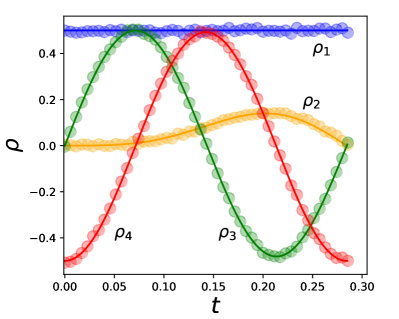
Figure 4: Density matrix coefficients as functions of time for the magnetic resonance Hamiltonian. The plots from the classical (continuous lines) and quantum (circles) computations are shown.

VI Example 1: one spin 1/2 particle subject to a time varying magnetic field

As a toy example, in this section we examine a spin $1/2$ particle in a varying magnetic field. The time evolution of the density matrix elements $\rho_{1}(t)$, $\rho_{2}(t)$, $\rho_{3}(t)$ and $\rho_{4}(t)$ were calculated by means of the classical and quantum algorithms. The Hamiltonian for this system is

$$H(t)=\omega_{1}\cos(\omega t)\sigma_{x}/2\\ -\omega_{1}\cos(\omega t+\phi)\sigma_{y}/2-\omega_{0}\sigma_{z}/2.$$ (80)

Projecting it onto the base formed by the Pauli matrices by means of Eq. (30) we obtain $a_{1}(t)=0$, $a_{2}(t)=\omega_{1}\cos(\omega t)/\sqrt{2}$, $a_{3}(t)=-\omega_{1}\cos(\omega t+\phi)/\sqrt{2}$ and $a_{4}(t)=\omega_{0}/\sqrt{2}$. If we assume that at $t=0$ the particle is in the lowest energy level, the initial condition for the density matrix must be

$$\rho(0)=\frac{1}{2}\left(I-\sigma_{z}\right).$$ (81)

The initial density matrix coefficients are thus obtained from Eq. (30) giving $\rho_{1}(0)=1/\sqrt{2}$, $\rho_{2}(0)=0$, $\rho_{3}(0)=0$ and $\rho_{4}(0)=-1/\sqrt{2}$. In this example we have set the following Hamiltonian parameters: $\omega=0.9$, $\omega_{0}=1$, $\omega=22.0$ and $\phi=\pi/2$.

In Fig. 4 we present the density matrix coefficients as a function of time calculated through the classical (continuous lines) and quantum (circles) algorithms. The quantum algorithm was executed in the IBM noisy quantum circuit (QASM) simulator. Each dot in the plot was obtained from a total of $16384$ shots. The figure shows that the classical and quantum algorithms are consistent.

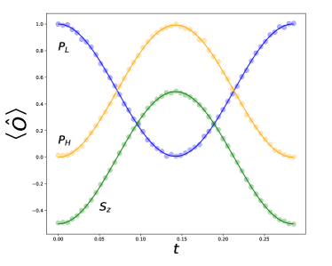
Figure 5: Expected values of the lowest energy level population, highest energy level population and spin projection along the $z$ axis. The classical and quantum computations are shown as solid lines and circles, respectively.

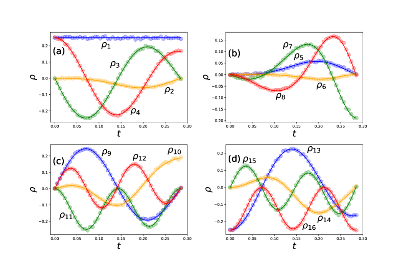
Figure 6: Density matrix coefficients as functions of time for the Hamiltonian corresponding to two spin 1/2 particles coupled through exchange interaction subject to a oscillating magnetic field. The classical and quantum computations are shown as solid lines and circles, respectively.

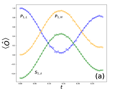
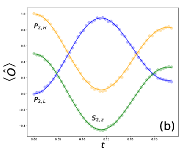
Figure 7: Expected values of the lowest energy level population, highest energy level population and spin projection along the $z$ axis for (a) the first and (b) second atoms. The classical and quantum computations are shown as solid lines and circles, respectively.

In order to illustrate how to calculate expected values using the density matrix coefficients and to further compare the classical and quantum algorithms Fig. 5 exhibits the expected values of the populations of the lowest and highest energy levels and the $z$ projection of the spin given by

$$P_{L}(t) = \mathrm{Tr}\left[\left|1\right\rangle\left\langle 1\right|\rho(t)\right],$$ (82)

$$P_{H}(t) = \mathrm{Tr}\left[\left|2\right\rangle\left\langle 2\right|\rho(t)\right],$$ (83)

$$S_{z}(t) = \mathrm{Tr}\left[\frac{1}{2}\sigma_{z}\rho(t)\right].$$ (84)

All the results in this section where also confirmed by directly solving the von Neumann equation (1) for the matrix elements of $\rho(t)$ and then projecting on to the elements of $\mathfrak{h}_{n}$ using Eq. (31).

VII Example 2: two spin 1/2 particles coupled through exchange interaction subject to a oscillating magnetic field.

In order to test a larger system, in this section we deal with the time evolution of two spin $1/2$ particles coupled through exchange interaction subject to a time-varying magnetic field. The Hamiltonian for two electron spins coupled through the exchange interaction characterized by $A$ and subject to a varying magnetic field is given by

$$H=\omega_{1}\cos(\omega t)\left(S_{x,1}+S_{x,2}\right)\\ +\omega_{1}\cos(\omega t+\phi)\left(S_{y,1}+S_{y,2}\right)+\omega_{0}\left(S_{z,1}+S_{z,2}\right)\\ +A\boldsymbol{S}_{1}\cdot\boldsymbol{S}_{2},$$ (85)

where $\boldsymbol{S}_{1}$ and $\boldsymbol{S}_{2}$ are the spin operators for the first and second particles, respectively. Projecting onto the base formed by the Pauli strings the non vanishing coefficients of the Hamiltonian are $a_{2}(t)=a_{5}(t)=\omega_{1}\cos(\omega t)$, $a_{3}(t)=a_{9}(t)=-\omega_{1}\cos(\omega t+\phi)$, $a_{4}(t)=a_{13}(t)=-\omega_{0}$ and $a_{6}(t)=a_{11}(t)=a_{16}(t)=A/2$.

The initial condition, that corresponds to both electrons being in the lowest energy level, is given by

$$\rho(0)=\frac{1}{2}\left(I-\sigma_{z}\right)\otimes\frac{1}{2}\left(I-\sigma_{z}\right).$$ (86)

The non vanishing coefficients corresponding to this condition are $\rho_{1}(0)=\rho_{4}(0)=-\rho_{13}(0)=-\rho_{16}(0)=1/2$. In this example the Hamiltonian parameters are $\omega=0.9$, $\omega_{0}=1$, $\omega=22.0$, $\phi=\pi/2$ and $A=3.0$.

In Fig. 6 we observe the $16$ density matrix coefficients as a function of time. Both classical and quantum computations are consistent. To further compare the classical and quantum algorithms Fig. 7 presents the expected values of the population corresponding to the lowest and highest energy levels of both atoms $P_{1,L}(t)$, $P_{1,H}(t)$, $P_{2,L}(t)$, $P_{2,H}(t)$ where

$$P_{1,L}(t) = \mathrm{Tr}\left[\left|1\right\rangle\left\langle 1\right|\otimes I\rho(t)\right],$$ (87)

$$P_{1,H}(t) = \mathrm{Tr}\left[\left|2\right\rangle\left\langle 2\right|\otimes I\rho(t)\right],$$ (88)

$$P_{2,L}(t) = \mathrm{Tr}\left[I\otimes\left|1\right\rangle\left\langle 1\right|\rho(t)\right],$$ (89)

$$P_{2,H}(t) = \mathrm{Tr}\left[I\otimes\left|2\right\rangle\left\langle 2\right|\rho(t)\right].$$ (90)

This figure also shows the expected values of the spin $z$ component $S_{z}$

$$S_{1,z}(t) = \mathrm{Tr}\left[\frac{1}{2}\sigma_{z}\otimes I\rho(t)\right],$$ (91)

$$S_{2,z}(t) = \mathrm{Tr}\left[I\otimes\frac{1}{2}\sigma_{z}\rho(t)\right],$$ (92)

where $I$ is the $2\times 2$ identity matrix.

As in the previous example, the coefficients of the density matrix where also confirmed by solving Eq. (1) and then projecting onto the elements of $\mathfrak{h}_{n}$ through Eq. (LABEL:eq:rhoprojection).

VIII Conclusions

In the present paper, a general framework to linearize the von-Neumann equation was developed. It mainly relies on the projection of the density matrix and the Hamiltonian on an operator base formed by the elements of a Lie algebra. For the particular case of $\mathfrak{q}_{n}$ the von-Neumann equation is mapped to the conventional Shrödinger-like equation (2), where the state vector $\left|\boldsymbol{\rho}(t)\right\rangle$ corresponds to the column stacked matrix elements of the density matrix $\rho(t)$ and the Hamiltonian to the superoperator $\mathcal{H}=I\otimes H(t)-H^{\top}(t)\otimes I$. It is shown that this is but one of the multiple ways of linearizing the von-Neumann equation. Other versions can be obtained by projecting onto different algebras. In the case of the Hermitian algebras $\mathfrak{h}_{n}$ the linearization yields a density matrix vector $\left|\boldsymbol{\rho}(t)\right\rangle$ with purely real entries which highly simplifies the quantum tomography of the final state vector. Moreover, it was proven that although the Hamiltonian superoperator has dimension $n\times n$, only $n$ generators are needed to build the time evolution operator considerably reducing the number of necessary quantum gates. Due to the unique properties of the Pauli strings the Hamiltonian gates can be implemented as a sequence of at most $n$ commuting Pauli gates. This presents two advantages: first, Pauli gates are easy to create in terms of Clifford gates and, second, no Trotterization is needed to mitigate errors considerably reducing the circuit depth.

All these notions were used to implement a quantum algorithm that solves the von-Neumann equation. The quantum algorithm was tested against the classical solution of the von Neumann equation for two toy Hamiltonians using the QASM simulator of IBMQ IBM giving identical results. Even though these algorithms were devised for the algebra whose elements are the Pauli strings, they can readily be adapted for any other Hermitian algebra.

We have seen in Eqs. (71) and (72) that the structure constants generate the time evolution of the density matrix through a series of unitary quantum gates. This framework thus gives us the flexibility to engineer the structure constants and consequently the required quantum gates by choosing the elements of the algebra.

This same scheme can also be applied to the analysis of the time evolution of open-quantum systems through the linearization of the Lindblad-Von Neumann master equation. This problem will be addressed elsewhere.

Appendix A Useful identities for the $\mathfrak{q}_{n}\otimes\mathfrak{q}_{n}$

In this appendix we prove that the Kronecker product of two matrices $B^{\top}\otimes A$ expanded in terms of the elements $Q_{i,j}$ of $\mathfrak{q}_{n}\otimes\mathfrak{q}_{n}$ can be related to the expansion in terms of $q_{k}\otimes q_{l}$ through

$$\Tr\left[Q_{i,j}^{\dagger}B^{\top}\otimes A\right]=\Tr\left[q_{i}^{\dagger}Aq_{j}B\right].$$ (93)

Expanding $A$ and $B$ in the right-hand side of (93) we find that

$$\Tr\left[q_{i}^{\dagger}Aq_{j}B\right]=\sum_{a,b}\Tr\left[q_{i}^{\dagger}q_{a}^{\dagger}q_{j}q_{b}\right]\Tr\left[q_{a}A\right]\Tr\left[q_{b}^{\dagger}B\right]\\ =\sum_{a,b}\Tr\left[q_{i}^{\dagger}q_{a}^{\dagger}q_{j}q_{b}\right]\Tr\left[q_{a}A\right]\Tr\left[q_{b}B^{\top}\right]\\ =\sum_{a,b}\Tr\left[q_{i}^{\dagger}q_{a}^{\dagger}q_{j}q_{b}\right]\Tr\left[q_{b}\otimes q_{a}B^{\top}\otimes A\right].$$ (94)

In the last step we have used $\Tr\left[q_{b}B^{\top}\right]=\Tr\left[q_{b}^{\dagger}B\right]$. Substituting the expansion of $q_{b}^{\dagger}\otimes q_{a}^{\dagger}$ in terms of the $Q_{r,s}$ as

$$q_{b}\otimes q_{a}=\sum_{k,l}\Tr\left[Q_{k,l}^{\dagger}q_{b}\otimes q_{a}\right]Q_{k,l}$$ (95)

into Eq. (94) we obtain

$$\Tr\left[q_{i}^{\dagger}Aq_{j}B\right]=\sum_{k,l,a,b}\Tr\left[q_{i}^{\dagger}q_{a}^{\dagger}q_{j}q_{b}\right]\Tr\left[Q_{k,l}^{\dagger}q_{b}\otimes q_{a}\right]\\ \times\Tr\left[Q_{k,l}B^{\top}\otimes A\right].$$ (96)

Only if $a$ and $b$ are given by (22) and (23), as stated by (21), the term $\Tr[Q_{k,l}^{\dagger}q_{b}\otimes q_{a}]=1$, otherwise $\Tr[Q_{k,l}^{\dagger}q_{b}\otimes q_{a}]=0$. Hence, the only non vanishing term from the sum in (96) is

$$\Tr\left[q_{i}^{\dagger}q_{a}^{\dagger}q_{j}q_{b}\right]=\sum_{p}\delta_{p,i_{2}}\delta_{i_{1},a_{2}}\delta_{a_{1},j_{1}}\delta_{j_{2},b_{1}}\delta_{b_{2},p}\\ =\delta_{i_{1},a_{2}}\delta_{a_{1},j_{1}}\delta_{j_{2},b_{1}}\delta_{b_{2},i_{2}}.$$ (97)

Plugging (18) and (19) in to the previous equation, one gets

$$\Tr\left[q_{i}^{\dagger}q_{a}^{\dagger}q_{j}q_{b}\right]=\sum_{p}\delta_{p,i_{2}}\delta_{i_{1},a_{2}}\delta_{a_{1},j_{1}}\delta_{j_{2},b_{1}}\delta_{b_{2},p}\\ =\delta_{i_{1},a_{2}}\delta_{a_{1},j_{1}}\delta_{j_{2},b_{1}}\delta_{b_{2},i_{2}}\\ =\delta_{(i-1)\bmod N+1,[(a-1)/N]+1}\\ \times\delta_{(a-1)\bmod N+1,(j-1)\bmod N+1}\\ \times\delta_{[(j-1)/N]+1,(b-1)\bmod N+1}\\ \times\delta_{[(b-1)/N]+1,[(i-1)/N]+1}.$$ (98)

Substituting the explicit expressions for $a$ and $b$ from (22) and (23) in the equation above yields

$$\Tr\left[q_{i}^{\dagger}q_{a}^{\dagger}q_{j}q_{b}\right]=\delta_{(i-1)\bmod N+1,(k-1)\bmod N+1}\\ \times\delta_{(l-1)\bmod N+1,(j-1)\bmod N+1}\\ \times\delta_{[(j-1)/N]+1,[(l-1)/N]+1}\\ \times\delta_{[(k-1)/N]+1,[(i-1)/N]+1}=\delta_{i,k}\delta_{j,l}.$$ (99)

Introducing this result in (96) we finally obtain (93).

Appendix B Useful properties of the Pauli strings algebra

In this appendix we derive useful properties for the Pauli strings algebra mainly to obtain recurrence relations that make the classical stage of the algorithm more efficient. Pauli strings have the form $(1/2)^{n/2}\sigma_{k_{1}}\otimes\sigma_{k_{2}}\dots\otimes\sigma_{k_{n}}$ where $\sigma_{0}$ is the $2\times 2$ identity matrix, $\sigma_{i}$ ($i=1,2,3$) are proportional to the standard Pauli matrices

$$h_{i}^{1}=\frac{1}{\sqrt{2}}\sigma_{i},$$ (100)

and the factor $1/\sqrt{2}$ is used to normalize the base to unity. Here we have adopted a notation where the superindex $n$ of the element $h_{i}^{n}$ indicates the number of qbits spanned by the algebra. The elements of algebras of higher dimension can be computed by sequentially taking the Kronecker product of the elements of lower dimensional algebras. For example, the elements of the algebra that spans two qbits may be obtained from the Kronecker product of the elements of the algebra corresponding to one qbit as

$$h_{i}^{2}=\frac{1}{\sqrt{2}}\sigma_{i_{1}}\otimes\frac{1}{\sqrt{2}}\sigma_{i_{2}}=h_{i_{1}}^{1}\otimes h_{i_{2}}^{1},$$ (101)

where $i=4(i_{1}-1)+i_{2}$, $i_{1},i_{2}=1,2,3,4$ and $i=1,2,\dots,16$. More generally, the algebra of $n+m$ qbits can be generated from the Kronecker product of the algebras of $n$ and $m$ qbits, i.e.,

$$h_{i}^{n+m}=h_{i_{1}}^{n}\otimes h_{i_{2}}^{m},$$ (102)

where

$$i = 2^{2m}(i_{1}-1)+i_{2},$$ (103)

$$i = 1,2,\dots,2^{2(n+m)},$$ (104)

$$i_{1} = 1,2,\dots,2^{2n},$$ (105)

$$i_{2} = 1,2,\dots,2^{2m}.$$ (106)

In particular, a base corresponding to an arbitrary number of qbits can be constructed by recursively applying

$$h_{i}^{n+1}=h_{i_{1}}^{n}\otimes h_{i_{2}}^{1},$$ (107)

where $i=4(i_{1}-1)+i_{2}$, $i=1,2,\dots,2^{2(n+1)}$, $i_{1}=1,2,\dots,2^{2n}$, $i_{2}=1,2,3,4$.

In this notation, the commutation of two elements of the algebra is given in terms of the structure constants as

$$\left[h_{i}^{n},h_{j}^{n}\right]=i\hbar\sum_{k=1}^{2^{2n}}c_{i,j,k}^{n}h_{k}^{n}.$$ (108)

Using the orthonormailty of this base, the explicit form of the structure constant is given as

$$c_{i,j,k}^{n}=\frac{1}{i\hbar}\Tr\left[\left[h_{i}^{n},h_{j}^{n}\right]h_{k}^{n}\right].$$ (109)

The structure constants $b_{i,j,k}^{n}$ ensued from taking the anticommutator as the Lie braket allow to express the anticommutator as

$$\left\{h_{i}^{n},h_{j}^{n}\right\}=\sum_{k=1}^{2^{2n}}b_{i,j,k}^{n}h_{k}^{n}.$$ (110)

Explicitly,

$$b_{i,j,k}^{n}=\Tr\left[\left\{h_{i}^{n},h_{j}^{n}\right\}h_{k}^{n}\right].$$ (111)

Although these do not play any role in the construction of the Hamiltonian gates, they will be very useful as auxiliary parameters in determining recurrence relations for $c_{i,j,k}^{n}$.

From the general commutator relations

$$\left[A_{1}\otimes A_{2},D_{1}\otimes D_{2}\right]=\frac{1}{2}\left[A_{1},A_{2}\right]\otimes\left\{D_{1},D_{2}\right\}\\ +\frac{1}{2}\left\{A_{1},A_{2}\right\}\otimes\left[D_{1},D_{2}\right],$$ (112)

$$\left\{A_{1}\otimes A_{2},D_{1}\otimes D_{2}\right\}=\frac{1}{2}\left[A_{1},A_{2}\right]\otimes\left[D_{1},D_{2}\right]\\ +\frac{1}{2}\left\{A_{1},A_{2}\right\}\otimes\left\{D_{1},D_{2}\right\},$$ (113)

if follows immediately that the commutator and anticommutator of an algebra of dimension $2^{2(n+m)}$ can be expressed in terms of the commutator and anticommutator of algebras of smaller dimensions $2^{2n}$ and $2^{2m}$ as

$$\left[h_{i}^{n+m},h_{j}^{n+m}\right]=\left[h_{i_{1}}^{n}\otimes h_{i_{n}}^{m},h_{j_{1}}^{n}\otimes h_{j_{2}}^{n}\right]\\ =\frac{1}{2}\left[h_{i_{1}}^{n},h_{j_{1}}^{m}\right]\otimes\left\{h_{i_{2}}^{m},h_{j_{2}}^{m}\right\}\\ +\frac{1}{2}\left\{h_{i_{1}}^{n},h_{j_{1}}^{n}\right\}\otimes\left[h_{i_{2}}^{m},h_{j_{2}}^{m}\right],$$ (114)

$$\left\{h_{i}^{n},h_{j}^{m}\right\}=\left\{h_{i_{1}}^{n}\otimes h_{i_{2}}^{m},h_{j_{1}}^{n}\otimes h_{j_{2}}^{n}\right\}\\ =\frac{1}{2}\left[h_{i_{1}}^{n},h_{j_{1}}^{m}\right]\otimes\left[h_{i_{2}}^{m},h_{j_{2}}^{m}\right]\\ +\frac{1}{2}\left\{h_{i_{1}}^{n},h_{j_{1}}^{n}\right\}\otimes\left\{h_{i_{2}}^{m},h_{j_{2}}^{m}\right\}.$$ (115)

Now we move on to how to workout recurrence relations for the structure constants. Multiplying both sides of (114) and (115) by $h_{k}^{n+m}=h_{k_{1}}^{n}\otimes h_{k_{2}}^{m}$ and using the definitions (109) and (111) we obtain the following recurrence relations

$$c_{i,j,k}^{n+m}=\frac{1}{2}\left(b_{i_{1},j_{1},k_{1}}^{n}c_{i_{2},j_{2},k_{2}}^{m}+c_{i_{1},j_{1},k_{1}}^{n}b_{i_{2},j_{2},k_{2}}^{m}\right),$$ (116)

$$b_{i,j,k}^{n+1}=\frac{1}{2}\left(b_{i_{1},j_{1},k_{1}}^{n}b_{i_{2},j_{2},k_{2}}^{m}-c_{i_{1},j_{1},k_{1}}^{n}c_{i_{2},j_{2},k_{2}}^{m}\right),$$ (117)

or more succintly

$$C_{k}^{n+m}=\frac{1}{2}\left(C_{k_{1}}^{n}\otimes B_{k_{2}}^{m}+B_{k_{1}}^{n}\otimes C_{k_{2}}^{m}\right),$$ (118)

$$B_{k}^{n+m}=\frac{1}{2}\left(B_{k_{1}}^{n}\otimes B_{k_{2}}^{m}-C_{k_{1}}^{n}\otimes C_{k_{2}}^{m}\right),$$ (119)

where $(C_{k}^{n})_{i,j}=c_{i,j,k}^{n}$ and $(B_{k}^{n})_{i,j}=b_{i,j,k}^{n}$. The use of these recurrence relations to obtain structure constants is far more efficient than the direct application of (109) and (111) because it avoids the tracing and all the matrix multiplications required by (109) and (111). For instance, one could initially calculate the structure constants for $n=1$ (one qbit) through (109) and (111), and then, by setting $m=1$ in (118) and (119) it is possible to recursively compute the commutors and anticommutors of progressively larger algebras.

In a similar fashion we are able compute recurrence relations for the coefficients $\Tr[C_{k}h_{i}^{(2)}]=\Tr[C_{k}^{n}h_{i}^{2n}]$ of the structure constants required by the Hamitlonian gate (75). To do so we substitute (119) with $m=1$ and $h_{i}^{2n}=h_{i_{1}}^{n}\otimes h_{i_{2}}^{n}$ into $\Tr[C_{k}^{n+1}h_{i}^{2(n+1)}]$ obtaining the recurrence relation

$$\Tr\left[C_{k}^{n+1}h_{i}^{2(n+1)}\right]=\frac{1}{2}\Tr\left[B_{k_{1}}^{n}h_{i_{1}}^{2n}\right]\Tr\left[C_{k_{2}}^{1}h_{i_{1}}^{2}\right]\\ +\frac{1}{2}\Tr\left[C_{k_{1}}^{n}h_{i_{1}}^{2n}\right]\Tr\left[B_{k_{1}}^{1}h_{i_{2}}^{2}\right].$$ (120)

Similarly $\Tr[B_{k}^{n+1}h_{i}^{2n}]$, also required by the expression above, can be computed as

$$\Tr\left[B_{k}^{n+1}h_{i}^{2(n+1)}\right]=\frac{1}{2}\Tr\left[B_{k_{1}}^{n}h_{i_{1}}^{2n}\right]\Tr\left[B_{k_{2}}^{1}h_{i_{1}}^{2}\right]\\ -\frac{1}{2}\Tr\left[C_{k_{1}}^{n}h_{i_{1}}^{2n}\right]\Tr\left[C_{k_{1}}^{1}h_{i_{2}}^{2}\right].$$ (121)

It only remains to prove that in the expansion of the Hamiltonian gate (75) the elements $h_{i}^{2n}$ with non-vanishing coefficients $\Tr[C_{k}^{n}h_{i}^{2n}]$ commute with each other. This can be easily proven by showing that the commutator of the projections of $C_{k}^{n}$ over two generic elements $h_{i}^{2n}$ and $h_{j}^{2n}$ vanishes, namely

$$\bigg{[}\Tr\left[C_{k}^{n}h_{i}^{2n}\right]h_{i}^{2n},\Tr\left[C_{k}^{n}h_{j}^{2n}\right]h_{j}^{2n}\bigg{]}=0.$$ (122)

By using Eq. (109) Eq. (122) takes the form

$$\bigg{[}\Tr\left[C_{k}^{n}h_{i}^{2n}\right]h_{i}^{2n}\,,\Tr\left[C_{k}^{n}h_{j}^{2n}\right]h_{j}^{2n}\bigg{]}\\ =i\hbar\Tr\left[C_{k}^{n}h_{i}^{2n}\right]\Tr\left[C_{k}^{n}h_{j}^{2n}\right]\sum_{m=1}^{2^{4n}}c_{i,j,m}^{2n}h_{m}^{2n}.$$ (123)

Then, multiplying both sides by $h_{l}^{2n}$ and tracing, we have

$$\Tr\left[C_{k}^{n}h_{i}^{2n}\right]\Tr\left[C_{k}^{n}h_{j}^{2n}\right]c_{i,j,l}^{2n}=0.$$ (124)

The values of a total of $\overbrace{2^{2n}}^{k}\times\overbrace{2^{4n}}^{i}\times\overbrace{2^{4n}}^{j}\times\overbrace{2^{4n}}^{l}=2^{14n}$ terms are needed to prove that. Even for a small number of qbits this is a challenging task. However, (124) can be recast in the form of a recurrence relation by substituting in it (118), (120) and (121) for which we find

$$\Tr\left[C_{k}^{n+1}h_{i}^{2(n+1)}\right]\Tr\left[C_{k}^{n+1}h_{j}^{2(n+1)}\right]c_{i,j,l}^{2(n+1)}=\frac{1}{8}\Tr\left[C_{k_{1}}^{n}h_{i_{1}}^{2n}\right]\Tr\left[C_{k_{1}}^{n}h_{j_{1}}^{2n}\right]c_{i_{1},j_{1},l_{1}}^{2n}\Tr\left[B_{k_{2}}^{1}h_{i_{2}}^{2}\right]\Tr\left[B_{k_{2}}^{1}h_{j_{2}}^{2}\right]b_{i_{2},j_{2},l_{2}}^{2}\\ +\frac{1}{8}\Tr\left[B_{k_{1}}^{n}h_{i_{1}}^{2n}\right]\Tr\left[B_{k_{1}}^{n}h_{j_{1}}^{2n}\right]c_{i_{1},j_{1},l_{1}}^{2n}\Tr\left[C_{k_{2}}^{1}h_{i_{2}}^{2}\right]\Tr\left[C_{k_{2}}^{1}h_{j_{2}}^{2}\right]b_{i_{2},j_{2},l_{2}}^{2}\\ +\frac{1}{8}\Tr\left[C_{k_{1}}^{n}h_{i_{1}}^{2n}\right]\Tr\left[B_{k_{1}}^{n}h_{j_{1}}^{2n}\right]b_{i_{1},j_{1},l_{1}}^{2n}\Tr\left[B_{k_{2}}^{1}h_{i_{2}}^{2}\right]\Tr\left[C_{k_{2}}^{1}h_{j_{2}}^{2}\right]c_{i_{2},j_{2},l_{2}}^{2}\\ +\frac{1}{8}\Tr\left[B_{k_{1}}^{n}h_{i_{1}}^{2n}\right]\Tr\left[C_{k_{1}}^{n}h_{j_{1}}^{2n}\right]b_{i_{1},j_{1},l_{1}}^{2n}\Tr\left[C_{k_{2}}^{1}h_{i_{2}}^{2}\right]\Tr\left[B_{k_{2}}^{1}h_{j_{2}}^{2}\right]c_{i_{2},j_{2},l_{2}}^{2}\\ +\frac{1}{8}\Tr\left[B_{k_{1}}^{n}h_{i_{1}}^{2n}\right]\Tr\left[B_{k_{1}}^{n}h_{j_{1}}^{2n}\right]b_{i_{1},j_{1},l_{1}}^{2n}\Tr\left[C_{k_{2}}^{1}h_{i_{2}}^{2}\right]\Tr\left[C_{k_{2}}^{1}h_{j_{2}}^{2}\right]c_{i_{2},j_{2},l_{2}}^{2}\\ +\frac{1}{8}\Tr\left[C_{k_{1}}^{n}h_{i_{1}}^{2n}\right]\Tr\left[C_{k_{1}}^{n}h_{j_{1}}^{2n}\right]b_{i_{1},j_{1},l_{1}}^{2n}\Tr\left[B_{k_{2}}^{1}h_{i_{2}}^{2}\right]\Tr\left[B_{k_{2}}^{1}h_{j_{2}}^{2}\right]c_{i_{2},j_{2},l_{2}}^{2}\\ +\frac{1}{8}\Tr\left[B_{k_{1}}^{n}h_{i_{1}}^{2n}\right]\Tr\left[C_{k_{1}}^{n}h_{j_{1}}^{2n}\right]c_{i_{1},j_{1},l_{1}}^{2n}\Tr\left[C_{k_{2}}^{1}h_{i_{2}}^{2}\right]\Tr\left[B_{k_{2}}^{1}h_{j_{2}}^{2}\right]b_{i_{2},j_{2},l_{2}}^{2}\\ +\frac{1}{8}\Tr\left[C_{k_{1}}^{n}h_{i_{1}}^{2n}\right]\Tr\left[B_{k_{1}}^{n}h_{j_{1}}^{2n}\right]c_{i_{1},j_{1},l_{1}}^{2n}\Tr\left[B_{k_{2}}^{1}h_{i_{2}}^{2}\right]\Tr\left[C_{k_{2}}^{1}h_{j_{2}}^{2}\right]b_{i_{2},j_{2},l_{2}}^{2}.$$ (125)

The last four lines of the previous equation vanish because, as can be demonstrated from the direct computation of the traces and structure constants,

$$\Tr\left[C_{k_{2}}^{1}h_{i_{2}}^{2}\right]\Tr\left[C_{k_{2}}^{1}h_{j_{2}}^{2}\right]c_{i_{2},j_{2},l_{2}}^{2}=\Tr\left[B_{k_{2}}^{1}h_{i_{2}}^{2}\right]\Tr\left[B_{k_{2}}^{1}h_{j_{2}}^{2}\right]c_{i_{2},j_{2},l_{2}}^{2}\\ =\Tr\left[C_{k_{2}}^{1}h_{i_{2}}^{2}\right]\Tr\left[B_{k_{2}}^{1}h_{j_{2}}^{2}\right]b_{i_{2},j_{2},l_{2}}^{2}=\Tr\left[B_{k_{2}}^{1}h_{i_{2}}^{2}\right]\Tr\left[C_{k_{2}}^{1}h_{j_{2}}^{2}\right]b_{i_{2},j_{2},l_{2}}^{2}=0.$$ (126)

In this way, Eq. (125) simplifies into

$$\Tr\left[C_{k}^{n+1}h_{i}^{2(n+1)}\right]\Tr\left[C_{k}^{n+1}h_{j}^{2(n+1)}\right]c_{i,j,l}^{2(n+1)}=\frac{1}{8}\Tr\left[C_{k_{1}}^{n}h_{i_{1}}^{2n}\right]\Tr\left[C_{k_{1}}^{n}h_{j_{1}}^{2n}\right]c_{i_{1},j_{1},l_{1}}^{2n}\Tr\left[B_{k_{2}}^{1}h_{i_{2}}^{2}\right]\Tr\left[B_{k_{2}}^{1}h_{j_{2}}^{2}\right]b_{i_{2},j_{2},l_{2}}^{2}\\ +\frac{1}{8}\Tr\left[B_{k_{1}}^{n}h_{i_{1}}^{2n}\right]\Tr\left[B_{k_{1}}^{n}h_{j_{1}}^{2n}\right]c_{i_{1},j_{1},l_{1}}^{2n}\Tr\left[C_{k_{2}}^{1}h_{i_{2}}^{2}\right]\Tr\left[C_{k_{2}}^{1}h_{j_{2}}^{2}\right]b_{i_{2},j_{2},l_{2}}^{2}\\ +\frac{1}{8}\Tr\left[C_{k_{1}}^{n}h_{i_{1}}^{2n}\right]\Tr\left[B_{k_{1}}^{n}h_{j_{1}}^{2n}\right]b_{i_{1},j_{1},l_{1}}^{2n}\Tr\left[B_{k_{2}}^{1}h_{i_{2}}^{2}\right]\Tr\left[C_{k_{2}}^{1}h_{j_{2}}^{2}\right]c_{i_{2},j_{2},l_{2}}^{2}\\ +\frac{1}{8}\Tr\left[B_{k_{1}}^{n}h_{i_{1}}^{2n}\right]\Tr\left[C_{k_{1}}^{n}h_{j_{1}}^{2n}\right]b_{i_{1},j_{1},l_{1}}^{2n}\Tr\left[C_{k_{2}}^{1}h_{i_{2}}^{2}\right]\Tr\left[B_{k_{2}}^{1}h_{j_{2}}^{2}\right]c_{i_{2},j_{2},l_{2}}^{2}.$$ (127)

For the recurrence relation (127) to be complete three more terms are needed: $\Tr\left[B_{k_{1}}^{n}h_{i_{1}}^{2n}\right]\Tr\left[B_{k_{1}}^{n}h_{j_{1}}^{2n}\right]c_{i_{1},j_{1},l_{1}}^{2n}$, $\Tr\left[C_{k_{1}}^{n}h_{i_{1}}^{2n}\right]\Tr\left[B_{k_{1}}^{n}h_{j_{1}}^{2n}\right]b_{i_{1},j_{1},l_{1}}^{2n}$ and $\Tr\left[B_{k_{1}}^{n}h_{i_{1}}^{2n}\right]\Tr\left[C_{k_{1}}^{n}h_{j_{1}}^{2n}\right]b_{i_{1},j_{1},l_{1}}^{2n}$. Following the same pathway as for Eq. (127), we obtain that the remaining recurrence relations are

$$\Tr\left[B_{k}^{n+1}h_{i}^{2(n+1)}\right]\Tr\left[B_{k}^{n+1}h_{j}^{2(n+1)}\right]c_{i,j,l}^{2(n+1)}=\frac{1}{8}\Tr\left[C_{k_{1}}^{n}h_{i_{1}}^{2n}\right]\Tr\left[C_{k_{1}}^{n}h_{j_{1}}^{2n}\right]c_{i_{1},j_{1},l_{1}}^{2n}\Tr\left[C_{k_{2}}^{1}h_{i_{2}}^{2}\right]\Tr\left[C_{k_{2}}^{1}h_{j_{2}}^{2}\right]b_{i_{2},j_{2},l_{2}}^{2}\\ +\frac{1}{8}\Tr\left[B_{k_{1}}^{n}h_{i_{1}}^{2n}\right]\Tr\left[B_{k_{1}}^{n}h_{j_{1}}^{2n}\right]c_{i_{1},j_{1},l_{1}}^{2n}\Tr\left[B_{k_{2}}^{1}h_{i_{2}}^{2}\right]\Tr\left[B_{k_{2}}^{1}h_{j_{2}}^{2}\right]b_{i_{2},j_{2},l_{2}}^{2}\\ -\frac{1}{8}\Tr\left[C_{k_{1}}^{n}h_{i_{1}}^{2n}\right]\Tr\left[B_{k_{1}}^{n}h_{j_{1}}^{2n}\right]b_{i_{1},j_{1},l_{1}}^{2n}\Tr\left[C_{k_{2}}^{1}h_{i_{2}}^{2}\right]\Tr\left[B_{k_{2}}^{1}h_{j_{2}}^{2}\right]c_{i_{2},j_{2},l_{2}}^{2}\\ -\frac{1}{8}\Tr\left[B_{k_{1}}^{n}h_{i_{1}}^{2n}\right]\Tr\left[C_{k_{1}}^{n}h_{j_{1}}^{2n}\right]b_{i_{1},j_{1},l_{1}}^{2n}\Tr\left[B_{k_{2}}^{1}h_{i_{2}}^{2}\right]\Tr\left[C_{k_{2}}^{1}h_{j_{2}}^{2}\right]c_{i_{2},j_{2},l_{2}}^{2},$$ (128)

$$\Tr\left[C_{k}^{n+1}h_{i}^{2(n+1)}\right]\Tr\left[B_{k}^{n+1}h_{j}^{2(n+1)}\right]b_{i,j,l}^{2(n+1)}=-\frac{1}{8}\Tr\left[C_{k_{1}}^{n}h_{i_{1}}^{2n}\right]\Tr\left[C_{k_{1}}^{n}h_{j_{1}}^{2n}\right]c_{i_{1},j_{1},l_{1}}^{2n}\Tr\left[B_{k_{2}}^{1}h_{i_{2}}^{2}\right]\Tr\left[C_{k_{2}}^{1}h_{j_{2}}^{2}\right]c_{i_{2},j_{2},l_{2}}^{2}\\ -\frac{1}{8}\Tr\left[B_{k_{1}}^{n}h_{i_{1}}^{2n}\right]\Tr\left[B_{k_{1}}^{n}h_{j_{1}}^{2n}\right]c_{i_{1},j_{1},l_{1}}^{2n}\Tr\left[C_{k_{2}}^{1}h_{i_{2}}^{2}\right]\Tr\left[B_{k_{2}}^{1}h_{j_{2}}^{2}\right]c_{i_{2},j_{2},l_{2}}^{2}\\ +\frac{1}{8}\Tr\left[C_{k_{1}}^{n}h_{i_{1}}^{2n}\right]\Tr\left[B_{k_{1}}^{n}h_{j_{1}}^{2n}\right]b_{i_{1},j_{1},l_{1}}^{2n}\Tr\left[B_{k_{2}}^{1}h_{i_{2}}^{2}\right]\Tr\left[B_{k_{2}}^{1}h_{j_{2}}^{2}\right]b_{i_{2},j_{2},l_{2}}^{2}\\ +\frac{1}{8}\Tr\left[B_{k_{1}}^{n}h_{i_{1}}^{2n}\right]\Tr\left[C_{k_{1}}^{n}h_{j_{1}}^{2n}\right]b_{i_{1},j_{1},l_{1}}^{2n}\Tr\left[C_{k_{2}}^{1}h_{i_{2}}^{2}\right]\Tr\left[C_{k_{2}}^{1}h_{j_{2}}^{2}\right]b_{i_{2},j_{2},l_{2}}^{2},$$ (129)

and

$$\Tr\left[B_{k}^{n+1}h_{i}^{2(n+1)}\right]\Tr\left[C_{k}^{n+1}h_{j}^{2(n+1)}\right]b_{i,j,l}^{2(n+1)}=\frac{1}{8}\Tr\left[C_{k_{1}}^{n}h_{i_{1}}^{2n}\right]\Tr\left[C_{k_{1}}^{n}h_{j_{1}}^{2n}\right]c_{i_{1},j_{1},l_{1}}^{2n}\Tr\left[C_{k_{2}}^{1}h_{i_{2}}^{2}\right]\Tr\left[B_{k_{2}}^{1}h_{j_{2}}^{2}\right]c_{i_{2},j_{2},l_{2}}^{2}\\ -\frac{1}{8}\Tr\left[B_{k_{1}}^{n}h_{i_{1}}^{2n}\right]\Tr\left[B_{k_{1}}^{n}h_{j_{1}}^{2n}\right]c_{i_{1},j_{1},l_{1}}^{2n}\Tr\left[B_{k_{2}}^{1}h_{i_{2}}^{2}\right]\Tr\left[C_{k_{2}}^{1}h_{j_{2}}^{2}\right]c_{i_{2},j_{2},l_{2}}^{2}\\ -\frac{1}{8}\Tr\left[C_{k_{1}}^{n}h_{i_{1}}^{2n}\right]\Tr\left[B_{k_{1}}^{n}h_{j_{1}}^{2n}\right]b_{i_{1},j_{1},l_{1}}^{2n}\Tr\left[C_{k_{2}}^{1}h_{i_{2}}^{2}\right]\Tr\left[C_{k_{2}}^{1}h_{j_{2}}^{2}\right]b_{i_{2},j_{2},l_{2}}^{2}\\ +\frac{1}{8}\Tr\left[B_{k_{1}}^{n}h_{i_{1}}^{2n}\right]\Tr\left[C_{k_{1}}^{n}h_{j_{1}}^{2n}\right]b_{i_{1},j_{1},l_{1}}^{2n}\Tr\left[B_{k_{2}}^{1}h_{i_{2}}^{2}\right]\Tr\left[B_{k_{2}}^{1}h_{j_{2}}^{2}\right]b_{i_{2},j_{2},l_{2}}^{2}.$$ (130)

By recursively inputing (126) into the four recurrence relations (127)-(130) it is readily verified that (127)-(130) vanish for any number $n$ of qbits . In particular, the fact that (127) is zero proves that the projections $\Tr[C_{k}^{n}h_{i}^{2n}]h_{i}^{2n}$ and $\Tr[C_{k}^{n}h_{j}^{2n}]h_{j}^{2n}$ in Eq. (122) indeed commute, which is an essential factor in expressing the Hamiltonian gates of Eq. (75) as a succession of Pauli gates .

References

Feynman (1982)R. P. Feynman, International Journal of Theoretical Physics 21 (1982).
Lloyd (1996)S. Lloyd, Science 273, 1073
(1996).
Nielsen and Chuang (2002)M. A. Nielsen and I. Chuang, “Quantum computation
and quantum information,” (2002).