PLAN: Variance-Aware Private Mean Estimation

Abstract.

Differentially private mean estimation is an important building block in privacy-preserving algorithms for data analysis and machine learning. Though the trade-off between privacy and utility is well understood in the worst case, many datasets exhibit structure that could potentially be exploited to yield better algorithms. In this paper we present Private Limit Adapted Noise (plan), a family of differentially private algorithms for mean estimation in the setting where inputs are independently sampled from a distribution $\mathcal{D}$ over $\mathbf{R}^{d}$, with coordinate-wise standard deviations $\boldsymbol{\sigma}\in\mathbf{R}^{d}$. Similar to mean estimation under Mahalanobis distance, plan tailors the shape of the noise to the shape of the data, but unlike previous algorithms the privacy budget is spent non-uniformly over the coordinates. Under a concentration assumption on $\mathcal{D}$, we show how to exploit skew in the vector $\boldsymbol{\sigma}$, obtaining a (zero-concentrated) differentially private mean estimate with $\ell_{2}$ error proportional to $\|\boldsymbol{\sigma}\|_{1}$. Previous work has either not taken $\boldsymbol{\sigma}$ into account, or measured error in Mahalanobis distance — in both cases resulting in $\ell_{2}$ error proportional to $\sqrt{d}\|\boldsymbol{\sigma}\|_{2}$, which can be up to a factor $\sqrt{d}$ larger. To verify the effectiveness of plan, we empirically evaluate accuracy on both synthetic and real world data.

1. Introduction

Differentially private mean estimation is an important building block in many algorithms, notably in for example implementations of private stochastic gradient descent (Abadi et al., 2016; Pichapati et al., 2019; Denisov et al., 2022). While differential privacy is an effective and popular definition for privacy-preserving data processing, privacy comes at a cost of accuracy, and striking a good trade-off between utility and privacy can be challenging. Achieving a good trade-off is especially hard for high-dimensional data, as the required noise that ensures privacy increases with the number of dimensions. Making matters worse, differential privacy operates on a worst-case basis. Adding noise naïvely may result in a one-size-fits-none noise scale that, although private, fails to give meaningful utility for many datasets.

Motivating example. Consider the following toy example: take a constant $q\in(0,1)$ and let $\lambda\ll 1/d$ be a value close to zero. We consider a set of vectors $\boldsymbol{x}^{(1)},\dots,\boldsymbol{x}^{(n)}\in\mathbf{R}^{d}$ where, independently,

$$\boldsymbol{x}^{(j)}=\begin{cases}(1,\lambda,\dots,\lambda)&\text{with probability }q\\ (0,0,\dots,0)&\text{with probability }1-q\enspace.\end{cases}$$

Though the nominal dimension is $d$, the distribution is “essentially 1-dimensional”. Thus, we should be able to release a private estimate of the mean $(q,\lambda q,\dots,\lambda q)$ with about the same precision as a scalar value with sensitivity 1. However, previous private mean estimation techniques either:

• add the same amount of noise to all $d$ dimensions, making the $\ell_{2}$ norm of the error a factor $\Theta(\sqrt{d})$ larger, or

• split the privacy budget evenly across the $d$ dimensions, making the noise added to the first coordinate a factor $\Theta(\sqrt{d})$ larger than in the scalar case.

Instead, we would like to adapt to the situation, and spend most of the privacy budget on the first coordinate while still keeping the noise on the remaining $d-1$ coordinates low. Dimension reduction using private PCA (Amin et al., 2019; Dwork et al., 2014; Hardt and Price, 2014) could be used, but we aim for something simpler and more general: to spend more budget on coordinates with higher variance.

We explore the design space of such variance-aware budget allocations and show that, perhaps surprisingly, the intuitive approach of splitting the budget across coordinates proportional to their spread (which is optimal for Mahalanobis distance (Brown et al., 2021)) is not optimal for $\ell_{p}$ errors. Using this insight, we design a family of algorithms, Private Limit Adapted Noise (plan), that distributes the privacy budget optimally. The contributions of this work cover both theoretical and practical ground:

• We present Private Limit Adapted Noise (plan) (Section 3), a family of algorithms for differentially private mean estimation for $\ell_{2}$ error, and its accompanying privacy and utility analysis (Section 4).

• We formalize, introduce, and exemplify the notion of ($\boldsymbol{\sigma},p$)-well concentrated distributions (Section 4 & Section 5) that allows for the study of variance-aware algorithms for mean estimation.

• We generalize the analysis of plan to hold for arbitrary $\ell_{p}$ error (Section 4.6).

• We prove that plan matches the utility of the current state-of-the-art algorithm (Huang et al., 2021) for differentially private mean estimation up to constant factors in expectation — without requiring computationally expensive random rotations (Section 6).

• We implement two instantiations of plan, for $\ell_{1}$ and $\ell_{2}$ error respectively, and empirically evaluate the algorithms on synthetic and real world datasets (Section 7).

Scope.

We consider the setting where we have independent samples $\boldsymbol{x}^{(1)},\dots,\boldsymbol{x}^{(n)}$ from a distribution $\mathcal{D}$ over $\mathbf{R}^{d}$, and use $\boldsymbol{\sigma}\in\mathbf{R}^{d}$ to denote the vector where $\boldsymbol{\sigma}_{i}$ is the standard deviation of the $i$th coordinate of a sample from $\mathcal{D}$. For mean estimation, error is often expressed in terms of Mahalanobis distance (Section 2.2), which is natural if $\mathcal{D}$ is a Gaussian distribution. Our objective is instead to estimate the mean $\boldsymbol{\mu}$ of $\mathcal{D}$ with small $\ell_{p}$ error. This is natural in other settings, for example if input vectors:

• represent probability distributions over $\{1,\dots,d\}$, so that $\ell_{1}$ error corresponds to variation distance, or

• are binary, so that $\ell_{1}$ and $\ell_{2}$ error corresponds to mean error and root mean square error, respectively, over $d$ counting queries.

Our exposition will focus primarily on the case of $\ell_{2}$ error, which is most easily compared to previous work.

plan’s privacy guarantees are expressed as $\rho$-zero-Concentrated Differential Privacy (zCDP), where similar results follow for other notions, such as approximate differential privacy (Lemma 2.3). We consider the number of inputs, $n$, fixed — the neighboring relation is changing one vector among the inputs.

In the non-private setting, the empirical mean $\tfrac{1}{n}\sum_{j}\boldsymbol{x}^{(j)}$ is known to yield the smallest $\ell_{2}$ error of size $O(\|\boldsymbol{\sigma}\|_{2}/\sqrt{n})$. We are interested in the situation where the privacy parameter $\rho$ is small enough that the sampling error of the empirical mean is dominated by the error introduced by differential privacy.

Our results.

We show, both theoretically and empirically, that a careful privacy budgeting can improve the $\ell_{p}$ error compared to existing methods when the vector $\boldsymbol{\sigma}$ is skewed. Some limitation, beyond bounded variance, is needed for the distribution $\mathcal{D}$. We say that $\mathcal{D}$ is $\boldsymbol{\sigma}$-well concentrated if, roughly speaking, the norm of distance to the mean $\boldsymbol{\mu}$ of vectors sampled from $\mathcal{D}$ is unlikely to be much larger than vectors sampled from a multivariate exponential distribution with standard deviations given by $\boldsymbol{\sigma}$ or some root of $\boldsymbol{\sigma}$. In the case $p=2$ our upper bound is particularly simple to state:

Theorem 1.1.

(simplified version) Suppose $\mathcal{D}$ is $\boldsymbol{\sigma}$-well concentrated and that we know $\boldsymbol{\hat{\sigma}}$ such that $\|\boldsymbol{\sigma}-\boldsymbol{\hat{\sigma}}\|_{\infty}<1/d$. Then for $n=\tilde{\Omega}\left(\max\left(\sqrt{d/\rho},\rho^{-1}\right)\right)$ there is a mean estimation algorithm that satisfies $\rho$-zCDP and has expected $\ell_{2}$ error

$$\tilde{O}(1+\|\boldsymbol{\sigma}\|_{2}/\sqrt{n}+\|\boldsymbol{\sigma}\|_{1}/(n\sqrt{\rho}))$$

with high probability, where $\tilde{O}$ suppresses polylogarithmic factors in error probability, $d$, $n$, and a bound on the $\ell_{\infty}$ norm of input vectors.

Comparing Theorem 1.1 to applying the Gaussian mechanism directly provides a useful example. Given the vectors $\boldsymbol{x}^{(1)},\dots,\boldsymbol{x}^{(n)}$ sampled from $\mathcal{N}(\boldsymbol{\mu},\Sigma)$ for $\Sigma=\text{diag}(\boldsymbol{\sigma^{2}})$ where $\|\boldsymbol{\mu}\|_{2}=O(\|\boldsymbol{\sigma}\|_{2})$, and clipping at $C=\Theta(\|\boldsymbol{\sigma}\|_{2})$, would give an $\ell_{2}$ error bound of

$$\tilde{O}(\|\boldsymbol{\sigma}\|_{2}/\sqrt{n}+\sqrt{d}\|\boldsymbol{\sigma}\|_{2}/(n\sqrt{\rho}))\enspace.$$

Crucially, Theorem 1.1 is never worse, but can be better than applying the Gaussian mechanism directly. The value of $\|\boldsymbol{\sigma}\|_{1}$ is in the interval $[\|\boldsymbol{\sigma}\|_{2},\sqrt{d}\|\boldsymbol{\sigma}\|_{2}]$, where a smaller value of $\|\boldsymbol{\sigma}\|_{1}$ indicates larger skew. Thus, Theorem 1.1 is strongest when $\boldsymbol{\sigma}$ has a skewed distribution such that $\|\boldsymbol{\sigma}\|_{1}$ is close to the lower bound of $\|\boldsymbol{\sigma}\|_{2}$, assuming that the privacy parameter $\rho$ is small enough that the error due to privacy dominates the sampling error.

2. Preliminaries

We provide privacy guarantees via zero-Concentrated Differential Privacy (zCDP) in the bounded setting, where the dataset has a fixed size, as defined in this section. Since previous work measure error using different distances measures, we give both the definition for $\ell_{p}$ error (which we use), as well as Mahalanobis distance. Lastly, we give an overview of private quantile estimation which is a central building block of our algorithm.

2.1. Differential privacy

Differential privacy (Dwork et al., 2006) is a statistical property of an algorithm that limits information leakage by introducing controlled randomness to the algorithm. Formally, differential privacy restricts how much the output distributions can differ between any neighboring datasets. We say that a pair of datasets are neighboring, denoted $x\sim x^{\prime}$, if and only if there exists an $j\in[n]$ such that $\boldsymbol{x}^{(i)}=\boldsymbol{x}^{\prime(i)}$ for all $i\neq j$.

Definition 2.1 ((Dwork et al., 2006) ($\varepsilon$, $\delta$)-Differential Privacy).

A randomized mechanism $\mathcal{M}$ satisfies ($\varepsilon$, $\delta$)-DP if and only if for all pairs of neighboring datasets $x\sim x^{\prime}$ and all set of outputs $Z$ we have

$$\Pr[\mathcal{M}(x)\in Z]\leq e^{\varepsilon}\Pr[\mathcal{M}(x^{\prime})\in Z]+\delta$$

Definition 2.2 ((Bun and Steinke, 2016) zero-Concentrated Differential Privacy (zCDP)).

Let $\mathcal{M}$ denote a randomized mechanism satisfying $\rho$-zCDP for any $\rho>0$. Then for all $\alpha>1$ and all pairs of neighboring datasets $x\sim x^{\prime}$ we have

$$D_{\alpha}\left(\mathcal{M}(x)||\mathcal{M}(x^{\prime})\right)\leq\rho\alpha,$$

where $D_{\alpha}(X||Y)$ denotes the $\alpha$-Rényi divergence between two distributions $X$ and $Y$.

Lemma 2.3 ((Bun and Steinke, 2016) zCDP to $(\varepsilon,\delta)$-DP conversion).

If $\mathcal{M}$ satisfies $\rho$-zCDP, then $\mathcal{M}$ is $(\varepsilon,\delta)$-DP for any $\delta>0$ and $\varepsilon=\rho+2\sqrt{\rho\log(1/\delta)}$.

Lemma 2.4 ((Bun and Steinke, 2016) Composition).

If $M_{1}$ and $M_{2}$ satisfy $\rho_{1}$-zCDP and $\rho_{2}$-zCDP, respectively. Then $M=(M_{1},M_{2})$ satisfies $(\rho_{1}+\rho_{2})$-zCDP.

The Gaussian Mechanism adds noise from a Gaussian distribution independently to each coordinate of a real-valued query output. The scale of the noise depends on the privacy parameter and the $\ell_{2}$-sensitivity denoted $\Delta_{2}$. A query $q$ has sensitivity $\Delta_{2}$ if for all $x\sim x^{\prime}$ we have $\|q(x)-q(x^{\prime})\|_{2}\leq\Delta_{2}$.

Lemma 2.5 ((Bun and Steinke, 2016) The Gaussian Mechanism).

If $q:\mathbf{R}^{n\times d}\rightarrow\mathbf{R}^{d}$ is a query with sensitivity $\Delta_{2}$ then releasing $\mathcal{N}(q(x),\frac{\Delta_{2}^{2}}{2\rho}\mathbf{I})$ satisfies $\rho$-zCDP.

2.2. Distance measures

Here we introduce the distance measures for the error of a mean estimate. Let $\boldsymbol{\tilde{\mu}}=\mathcal{M}(x)$ denote the mean estimate of a distribution with mean $\boldsymbol{\mu}$. We measure the utility of our mechanism in terms of expected $\ell_{p}$ error as defined below. Here $p$ is a parameter of our mechanism where the most common values for $p$ are $1$ (Manhattan distance), and $2$ (Euclidean distance).

Definition 2.6 ($\ell_{p}$ error).

For any real value $p\geq 1$ the $\ell_{p}$ error is

$$\|\boldsymbol{\tilde{\mu}}-\boldsymbol{\mu}\|_{p}=\left(\sum_{i=1}^{d}|\tilde{\mu}_{i}-\mu_{i}|^{p}\right)^{1/p}$$

Note that we sometimes present error guarantees in the form of the $p$th moment, i.e. $\mathbf{E}[\|\boldsymbol{\tilde{\mu}}-\boldsymbol{\mu}\|_{p}^{p}]$, when it follows naturally from the analysis. Notice that the $p$th moment bounds the expected $\ell_{p}$ error for any $p\geq 1$ as $\mathbf{E}[\|\boldsymbol{\tilde{\mu}}-\boldsymbol{\mu}\|_{p}]\leq(\mathbf{E}[\|\boldsymbol{\tilde{\mu}}-\boldsymbol{\mu}\|_{p}^{p}])^{1/p}$.

As stated in Section 8 several previous work on mean estimates measure error in Mahalanobis distance. Although this is not the focus of our work we include the definition here for completeness. A key difference between Mahalanobis distance measure and $\ell_{p}$ error is that the directions are weighted by the uncertainty of the underlying data. We weight the error in all coordinates equally.

Definition 2.7 (Mahalanobis distance).

The error in Mahalanobis distance of a mean estimate for a distribution with covariance matrix $\Sigma$ is defined as

$$\|\boldsymbol{\tilde{\mu}}-\boldsymbol{\mu}\|_{\Sigma}=\|\Sigma^{-1/2}(\boldsymbol{\tilde{\mu}}-\boldsymbol{\mu})\|_{2}$$

2.3. Private quantile estimation

Our work builds on using differentially private quantiles, whose rank error (i.e. how many elements away from the desired quantile the output is) we will define for our utility analysis. When estimating the $q$’th quantiles of a sequence $\boldsymbol{z}^{(1)}\dots\boldsymbol{z}^{(n)}$ with $\boldsymbol{z}^{(j)}\in\mathbf{R}^{d}$, we ideally return a vector $\boldsymbol{\tilde{z}}\in\mathbf{R}^{d}$ such that for each coordinate $i$ we have $|\{j\in[n]:\boldsymbol{z}_{i}^{(j)}\leq\boldsymbol{\tilde{z}}_{i}\}|/n=q$. We use the notation $\textsc{PrivQuantile}_{\rho}^{M}(\boldsymbol{z}^{(1)}\dots\boldsymbol{z}^{(n)},q)$ to denote a $\rho$-zCDP mechanism that estimates the $q$’th quantiles of $\boldsymbol{z}^{(1)}\dots\boldsymbol{z}^{(n)}$ where each coordinate is bounded to $[-M,M]$.

There are multiple applicable choices for the instantiation of PrivQuantile from the literature, e.g. (Smith, 2011; Huang et al., 2021; Kaplan et al., 2022). In this paper we will use the binary search based quantile (Smith, 2011; Huang et al., 2021) for our utility analysis (Section 4), and the exponential mechanism based quantile by Kaplan et al. (2022) in our empirical evaluation (Section 7). Note that the choice of instantiation of PrivQuantile has no effect on the privacy analysis of plan. The binary search based method gives us cleaner theoretical results because the error guarantees of the exponential mechanism based technique is highly data-dependent, and the error is large for worst-case input. Empirically, however, the exponential mechanism based quantile is more robust, which is why we use it in our experiments.

The binary search based quantile subroutine performs a binary search over the interval $[-M,M]$. At each step of the search, branching is based on a quantile estimate for the midpoint of the current interval. Since branching must be performed privately the privacy budget needs to be partitioned in advance, this limits the binary search to $T$ iterations. Huang et al. (2021) describes the algorithm for discrete input where $T$ is the base 2 logarithm of the size of input domain. Treating $T$ as a parameter of the algorithm gives us the following guarantees for $1$-dimensional input.

Lemma 2.8 (Follows from Huang et al. (2021, Theorem 1)).

PrivQuantile satisfies $\rho^{\prime}$-zCDP and with probability at least $1-\beta$ it returns an interval containing at least one point with rank error bounded by $\sqrt{T\log(T/\beta)/(2\rho^{\prime})}$.

When estimating the quantiles of multiple dimensions, we split the privacy budget evenly across each dimensions such that $\rho^{\prime}=\rho/d$ for each invocation of PrivQuantile. By composition releasing all quantiles satisfies $\rho$-zCDP.

Lemma 2.9.

With probability at least $1-\beta$, $\textsc{PrivQuantile}_{\rho}^{M}$ returns a point that for all coordinates is within a distance of $M2^{-T}$ of a point with rank error at most $\sqrt{dT\log(Td/\beta)/2\rho}$ for the desired quantile.

Proof.

Running binary search for $T$ iterations splits up the range $[-M,M]$ in $2^{T}$ evenly sized intervals. By a union bound there is a point with claimed rank error in each of the intervals returned by PrivQuantile. Returning the midpoint of each interval ensures we are at most distance $M2^{-T}$ from said point. ∎

Throughout this paper, we set $T=\log_{2}(M)$ unless otherwise specified such that the error distance of Lemma 2.9 is $1$.

3. Algorithm

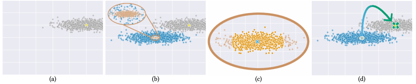
Figure 1. Step-by-step illustration of plan (Algorithm 1): (a) Raw data, with statistical mean (yellow star), (b) Recentering (blue) and scaling (orange) corresponding to 4, (c) Clipping, as determined by 6, (d) Private mean (green cross).

Conceptually, Private Limit Adapted Noise (plan) is a data-aware family of algorithms that exploits variance in the input data to tailor noise to the specific data at hand. Since it is a family of algorithms, a plan needs to be instantiated for a given problem domain, i.e. for a specific $\ell_{p}$ error and data distribution. In Section 7 we showcase two such instantiations, using $\ell_{1}$ error for binary data, and using $\ell_{2}$ for Gaussian data. Pseudocode for plan is shown in Algorithm 1, and a step-by-step illustration of plan is provided in Figure 1.

3.1. plan overview

Based on the input data (1, Figure 1 (a)) plan first computes a private, rough, approximate mean $\boldsymbol{\tilde{\mu}}$ (3). plan then recenters the data around $\boldsymbol{\tilde{\mu}}$, and scales the data (4, Figure 1 (b)) according to an estimate on the variance $\boldsymbol{\hat{\sigma}}^{2}$ — this scaling allows the privacy budget to be spent unevenly across dimensions. Next, plan clips inputs to a carefully chosen ellipsoid (6, Figure 1 (c)) centered around $\boldsymbol{\tilde{\mu}}$ that most data points fall within. The size of the ellipsoid is determined privately based on the data (5). Finally, plan adds sufficient Gaussian noise (7) to make the contribution of each clipped input differentially private, and transforms the results back to the original format (Figure 1 (d)). Each of these techniques have been used for private mean estimation before — we show that choosing the ellipsoid differently leads to smaller $\ell_{p}$ error.

Algorithm 1 plan

1:Input: $\boldsymbol{x}^{(1)},\dots,\boldsymbol{x}^{(n)}\in\mathbf{R}^{d}$, estimate $\boldsymbol{\hat{\sigma}}^{2}\in\mathbf{R}^{d}$

2:Parameters: $M,p,\rho_{1},\rho_{2},\rho_{3}$

3:$\boldsymbol{\tilde{\mu}}\leftarrow\textsc{PrivQuantile}_{\rho_{1}}^{M}(\boldsymbol{x}^{(1)},\dots,\boldsymbol{x}^{(n)},1/2)$

4:$\boldsymbol{y}^{(j)}\leftarrow(\boldsymbol{x}^{(j)}-\boldsymbol{\tilde{\mu}})\,\hat{\Sigma}^{-1/(p+2)}$ for $j=1,\dots,n$

5:$k\leftarrow\sqrt{n}+\Theta\left(\sqrt{1/\rho_{2}}\right)$

6:$C\leftarrow\textsc{PrivQuantile}_{\rho_{2}}^{M\sqrt{d}}(\|\boldsymbol{y}^{(1)}\|_{2},\dots,\|\boldsymbol{y}^{(n)}\|_{2},\tfrac{n-k}{n})$

7:sample $\boldsymbol{\eta}\sim\mathcal{N}(\mathbf{0},\frac{2C^{2}}{\rho_{3}}\mathbf{I})$

8:return $\boldsymbol{\tilde{\mu}}+\tfrac{1}{n}\left(\sum_{j}\min\left\{\frac{C}{\|\boldsymbol{y}^{(j)}\|_{2}},1\right\}\boldsymbol{y}^{(j)}+\boldsymbol{\eta}\right)\hat{\Sigma}^{1/(p+2)}$

3.2. plan building blocks

Like Instance-optimal mean estimation (iome) (Huang et al., 2021), our algorithm computes a rough estimate of the mean as a private estimate $\boldsymbol{\tilde{\mu}}\in\mathbf{R}^{d}$ of the coordinate-wise median. This step uses the assumption that all coordinates are in the interval $[-M,M]$. It is known that a finite output domain is needed for private quantile selection to be possible (Bun et al., 2015). Suppose $\ell_{p}$ is the error measure we are aiming to minimize. The next step is to scale coordinates by multiplying with the diagonal matrix $\hat{\Sigma}^{-1/(p+2)}$, where $\hat{\Sigma}=\text{diag}(\boldsymbol{\hat{\sigma}}^{2})$ is the diagonal matrix of variance estimates $\boldsymbol{\hat{\sigma}}^{2}$.

Note that since $\hat{\Sigma}$ is a diagonal matrix, it is not necessarily close to the covariance matrix of $\mathcal{D}$ outside of the diagonal. Note that for $p=2$ the exponent of $\hat{\Sigma}$ is $-1/4$, which is different from the exponent of $-1/2$ that would be used in order to compute an estimate with small Mahalanobis distance.

The scaling stretches the $i$th coordinate by a factor $\hat{\sigma}_{i}^{-2/(p+2)}$. Since $\hat{\sigma}^{2}_{i}\approx\sigma^{2}_{i}$ this changes the standard deviation on the $i$th coordinate from $\sigma_{i}$ to roughly $\sigma_{i}^{p/(p+2)}$. Next, we compute vectors $\boldsymbol{y}^{(j)}$ that represent the (stretched) differences $\boldsymbol{x}^{(j)}-\boldsymbol{\tilde{\mu}}$. Conceptually, we now want to estimate the mean of $\boldsymbol{y}^{(1)},\dots,\boldsymbol{y}^{(n)}$, which in turn implies an estimate of $(\tfrac{1}{n}\sum_{j}\boldsymbol{x}^{(j)})-\boldsymbol{\tilde{\mu}}$. The mean of $\boldsymbol{y}^{(1)},\dots,\boldsymbol{y}^{(n)}$ is estimated In order to find a suitable scaling of the noise we privately find a quantile $C$ of the lengths $\|\boldsymbol{y}^{(1)}\|_{2},\dots,\|\boldsymbol{y}^{(n)}\|_{2}$ (all shorter than $M\sqrt{d}$ by assumption) such that approximately $k$ vectors have length larger than $C$, and clip vectors to length at most $C$. Clipping, private mean estimation, scaling, and adding back $\boldsymbol{\tilde{\mu}}$ is all condensed in the estimator in 8 of Algorithm 1.

4. Analysis

Assumptions:

• We assume that for a known parameter $M$, all inputs are in $\boldsymbol{x}^{(j)}\in[-M,M]^{d}$ for $j=1,\dots,n$. (If this is not the case, the algorithm will clip inputs to this cube, introducing additional clipping error.) Also, we assume that data has been scaled sufficiently such that $\sigma_{i}\geq 1$ for $i=1,\dots,d$ (this can be enforced by adding independent noise of variance $1$ to each coordinate of inputs).

• We are given a vector $\boldsymbol{\hat{\sigma}}\in\mathbf{R}^{d}$ such that

  (1) $$\sigma_{i}\leq\hat{\sigma}_{i}<\sigma_{i}+\|\boldsymbol{\sigma}\|_{1}/d\enspace.$$

  If no such vector is known we will have to compute it, spending part of the privacy budget, but we consider this a separate question.

Definition 4.1.

Consider a distribution $\mathcal{D}$ over $\mathbf{R}^{d}$, denote the mean and standard deviation of the $i$th coordinate by $\mu_{i}$ and $\sigma_{i}$, respectively. We say that $\mathcal{D}$ is $\boldsymbol{\sigma}$-well concentrated if for any vector $\boldsymbol{\hat{\sigma}}\in\mathbf{R}^{d}$ with $\sigma_{i}\leq\hat{\sigma}_{i}<\sigma_{i}+\|\boldsymbol{\sigma}\|_{1}/d$, the following holds for $t>1$

(2) $$\Pr_{X\sim\mathcal{D}}\left[\sum_{i=1}^{d}(X_{i}-\mu_{i})^{2}>t\|\boldsymbol{\sigma}\|_{2}^{2}\right]=\exp(-\tilde{\Omega}(t))$$

(3) $$\Pr_{X\sim\mathcal{D}}\left[\sum_{i=1}^{d}(X_{i}-\mu_{i})^{2}/\hat{\sigma}_{i}>t\|\boldsymbol{\sigma}\|_{1}\right]=\exp(-\tilde{\Omega}(t))\enspace.$$

Intuitively, these assumptions require concentration of measure of the norms before and after scaling.

4.1. Analysis outline

We will show that plan returns a private mean estimate that, assuming $\mathcal{D}$ is $\boldsymbol{\sigma}$-well concentrated, has small expected $\ell_{p}$ error with probability at least $1-\beta$. All probabilities are over the joint distribution of the input samples and the randomness of the plan mechanism. For simplicity we focus on the case $p=2$, but the analysis extends to any $p\geq 1$ as we will show at the end of this section.

Privacy.

It is not hard to see that plan satisfies $\rho$-zCDP with $\rho=\rho_{1}+\rho_{2}+\rho_{3}$: The computation of $\boldsymbol{\tilde{\mu}}$ satisfies $\rho_{1}$-zCDP and the computation of $C$ satisfies $\rho_{2}$-zCDP by definition of PrivQuantile. Finally, given the values $C$ and $\boldsymbol{\tilde{\mu}}$ the $\ell_{2}$-sensitivity of $\sum_{j}\min\left\{\frac{C}{\|\boldsymbol{y}^{(j)}\|_{2}},1\right\}\boldsymbol{y}^{(j)}$ with respect to an input $\boldsymbol{x}^{(j)}$ is $2C$, so adding Gaussian noise with variance $2C^{2}/\rho_{3}$ gives a $\rho_{3}$-zCDP mean estimate. By composition, and since the returned estimator is a post-processing of these private values, the estimator is $\rho$-zCDP with $\rho=\rho_{1}+\rho_{2}+\rho_{3}$.

Utility.

It is known that mean estimation in $\mathbf{R}^{d}$ requires $n=\Omega(\sqrt{d/\rho})$ samples to achieve meaningful utility (Huang et al., 2021; Kamath et al., 2019). Thus we will assume that $n$ is sufficiently large, $n=\tilde{\Omega}(\sqrt{d/\rho})$, where the $\tilde{\Omega}$ notation hides polylogarithmic factors in $d$, $\beta$, and $M$. Let $\hat{\Sigma}$ denote the scaling matrix $\text{diag}(\boldsymbol{\hat{\sigma}}^{2})$. In the following, we assume that $\rho_{1},\rho_{2},\rho_{3}$ are fixed fractions of $\rho$.

The utility analysis has three parts:

1. First, we argue that $|\tilde{\mu}_{i}-\mu_{i}|<3\sigma_{i}$ for all $i=1,\dots,d$ with high probability.

2. Let $J$ denote the set of indices for which $\|\boldsymbol{y}^{(j)}\|_{2}>C$. We argue that with high probability,

   $$\sum_{j\in J}\|\boldsymbol{x}^{(j)}-\boldsymbol{\tilde{\mu}}\|_{2}=\tilde{O}\left(\left(k+\sqrt{\tfrac{1}{\rho}}\right)\|\boldsymbol{\sigma}\|_{2}\right),$$

   bounding the error due to clipping.

3. Finally, we argue that with high probability

   $$\left\|\boldsymbol{\eta}\,\hat{\Sigma}^{\tfrac{1}{p+2}}\right\|^{2}_{2}=\tilde{O}(\|\boldsymbol{\sigma}\|_{1}^{2}/\rho),$$

   bounding the error due to Gaussian noise.

4.2. Part 1: Bounding $|\boldsymbol{\tilde{\mu}}-\boldsymbol{\mu}|$

In the following $K$ is a universal constant chosen to be sufficiently large.

Lemma 4.2.

Assuming $n>K\sqrt{d/\rho}\log(d/\beta)\log(M)$ then with probability $1-\beta$, the coordinate-wise median ${\tilde{\mu}_{i}}$ satisfies ${\tilde{\mu}}_{i}\in[{\mu}_{i}-3{\sigma}_{i},{\mu}_{i}+3{\sigma}_{i}]$ for all $i=1,\dots,d$.

Proof.

Sample $X=(X_{1},\ldots,X_{d})\sim\mathcal{D}$. By Chebychev’s inequality, for each $i$ with $1\leq i\leq d$:

$$\Pr[|X_{i}{\mu}_{i}|\leq 2{\sigma}_{i}]\geq 1-\frac{{\sigma}_{i}^{2}}{(2{\sigma}_{i})^{2}}=3/4\enspace.$$

Fixing $i$, these events are independent for $j=1,\dots,n$ so by a Chernoff bound with probability $1-\exp(-\Omega(n))$ there are at least $\tfrac{2}{3}n$ indices $j$ such that $|X^{(j)}_{i}-{\mu}_{i}|\leq 2{\sigma}_{i}$. Condition on the event that this is true for $i=1,\dots,d$.

If the rank error of the median estimate ${\tilde{\mu}}_{i}$ is smaller than $n/6$, ${\tilde{\mu}}_{i}\in[{\mu}_{i}-3{\sigma}_{i},{\mu}_{i}+3{\sigma}_{i}]$, using the assumption that ${\sigma}_{i}\geq 1$. By Lemma 2.9 this is true for every $i$ with probability at least $1-\beta$, given our assumption on $n$ and $K$ if $K$ is a sufficiently large constant. ∎

4.3. Part 2: Bounding clipping error

Let $J=\{j\in\{1,\dots,n\}\;|\;\|\boldsymbol{y}^{(j)}\|_{2}>C\}$ denote the set of indices of vectors affected by clipping in plan. By the triangle inequality and assuming the bound of part 1 holds,

$$\sum_{j\in J}\left\|(\boldsymbol{x}^{(j)}-\boldsymbol{\tilde{\mu}})\right\|_{2} \leq\sum_{j\in J}\left\|(\boldsymbol{x}^{(j)}-\boldsymbol{\mu})\right\|_{2}+|J|\cdot\left\|\boldsymbol{\mu}-\boldsymbol{\tilde{\mu}}\right\|_{2}$$

$$\leq\sum_{j\in J}\left\|(\boldsymbol{x}^{(j)}-\boldsymbol{\mu})\right\|_{2}+3|J|\cdot\|\boldsymbol{\sigma}\|_{2}\enspace.$$

By assumption (2) the probability that $\|\boldsymbol{x}^{(j)}-\boldsymbol{\mu}\|_{2}^{2}>t\|\boldsymbol{\sigma}\|_{2}^{2}$ is exponentially decreasing in $t$, so setting $t=\tilde{\Omega}(\log^{2}(n/\beta))$ we have $\|\boldsymbol{x}^{(j)}-\boldsymbol{\mu}\|_{2}=\tilde{O}(\|\boldsymbol{\sigma}\|_{2})$ for all $j=1,\dots,n$ with probability at least $1-\beta$. Using the triangle inequality again we can now bound

$$\sum_{j\in J}\|\boldsymbol{x}^{(j)}-\boldsymbol{\mu}\|_{2}=\tilde{O}(|J|\cdot\|\boldsymbol{\sigma}\|_{2})\enspace.$$

Since $\left\|\boldsymbol{y}^{(j)}\right\|_{2}\leq M\sqrt{d}$, by Lemma 2.8, with probability at least $1-\beta$ (over the random choices of the private quantile selection algorithm) there are at most $\tilde{O}\left(k+\sqrt{\tfrac{1}{\rho}}\right)$ vectors $\boldsymbol{y}^{(j)}$ for which $\|\boldsymbol{y}^{(j)}\|_{2}>C$. So with probability at least $1-\beta$ we have $|J|=\tilde{O}\left(k+\sqrt{\tfrac{1}{\rho}}\right)$, and using the bounds above we get

$$\sum_{j\in J}\|\boldsymbol{x}^{(j)}-\boldsymbol{\tilde{\mu}}\|_{2}=\tilde{O}(|J|\cdot\|\boldsymbol{\sigma}\|_{2})=\tilde{O}\left(\left(k+\sqrt{\tfrac{1}{\rho}}\right)\|\boldsymbol{\sigma}\|_{2}\right)\enspace.$$

4.4. Part 3: Bounding noise

By triangle inequality:

$$\|\boldsymbol{y}^{(j)}\|_{2} =\left\|(\boldsymbol{x}^{(j)}-\boldsymbol{\tilde{\mu}})\,\hat{\Sigma}^{-\tfrac{1}{p+2}}\right\|_{2}$$

$$\leq\left\|(\boldsymbol{x}^{(j)}-\boldsymbol{\mu})\,\hat{\Sigma}^{-\tfrac{1}{p+2}}\right\|_{2}+\left\|(\boldsymbol{\mu}-\boldsymbol{\tilde{\mu}})\,\hat{\Sigma}^{-\tfrac{1}{p+2}}\right\|_{2}$$

For $p=2$, the $i$th coordinate of $(\boldsymbol{x}^{(j)}-\boldsymbol{\mu})\,\hat{\Sigma}^{-1/(p+2)}$ equals $({x}^{(j)}_{i}-{\mu}_{i})/\sqrt{{\hat{\sigma}}_{i}}$, so assumption (3) implies that the length of the first vector is $\tilde{O}(\sqrt{\|\boldsymbol{\sigma}\|_{1}})$ with probability at least $1-\beta/2$. From part 1 we know (again for $p=2$) that the $i$th coordinate of $(\boldsymbol{\mu}-\boldsymbol{\tilde{\mu}})\,\hat{\Sigma}^{-1/(p+2)}$ has absolute value at most

$$3{\sigma}_{i}/\sqrt{{\hat{\sigma}}_{i}}\leq 3\sqrt{{\sigma}_{i}},$$

where the inequality uses the lower bound on ${\hat{\sigma}}_{i}$ in assumption (1). So $\|(\boldsymbol{\mu}-\boldsymbol{\tilde{\mu}})\,\hat{\Sigma}^{-1/(p+2)}\|_{2}\leq 3\sqrt{\|\boldsymbol{\sigma}\|_{1}}$, and we get that $\|\boldsymbol{y}^{(j)}\|_{2}=\tilde{O}(\sqrt{\|\boldsymbol{\sigma}\|_{1}})$ for all $j$ with probability at least $1-\beta/2$.

The value of $C$ is bounded by the maximum length of a vector $\|\boldsymbol{y}^{(j)}\|_{2}$, and thus by a union bound, with probability at least $1-\beta$, $C^{2}=\tilde{O}(\|\boldsymbol{\sigma}\|_{1})$. The scaled noise vector $\boldsymbol{\eta}\,\hat{\Sigma}^{1/(p+2)}$ has distribution $\mathcal{N}(\boldsymbol{0},\frac{2C^{2}}{\rho_{3}}\hat{\Sigma}^{1/(p+2)})$, so using ${\hat{\sigma}}_{i}\leq{\sigma}_{i}+\|\boldsymbol{\sigma}\|_{1}/d$ from assumption (1), for $p=2$:

$$\mathbf{E}[\|\boldsymbol{\eta}\,\hat{\Sigma}^{1/(p+2)}\|_{2}^{2}] =\tfrac{2C^{2}}{\rho_{3}}\sum_{i=1}^{d}\hat{\Sigma}_{ii}^{2/(p+2)}$$

$$=\tfrac{2C^{2}}{\rho_{3}}\sum_{i=1}^{d}\hat{{\sigma}}_{i}$$

$$\leq\tfrac{2C^{2}}{\rho_{3}}\sum_{i=1}^{d}({\sigma}_{i}+\|\boldsymbol{\sigma}\|_{1}/d)=\tilde{O}(\|\boldsymbol{\sigma}\|_{1}^{2}/\rho_{3})\enspace.$$

4.5. Proof of Theorem 1.1

The output of plan can be written as

$$\tfrac{1}{n}\sum_{j=1}^{n}\boldsymbol{x}^{(j)}-\tfrac{1}{n}\sum_{j\in J}\tfrac{\|\boldsymbol{y}^{(j)}\|_{2}-C}{\|\boldsymbol{y}^{(j)}\|_{2}}\,(\boldsymbol{x}^{(j)}-\boldsymbol{\tilde{\mu}})+\tfrac{1}{n}\boldsymbol{\eta}\,\hat{\Sigma}^{1/(p+2)}$$

Using that $\tfrac{\|\boldsymbol{y}^{(j)}\|_{2}-C}{\|\boldsymbol{y}^{(j)}\|_{2}}<1$ for $j\in J$ and the triangle inequality, the $\ell_{2}$ estimation error of plan can thus be bounded as

$$\left\|\tfrac{1}{n}\sum_{j=1}^{n}\boldsymbol{x}^{(j)}-\boldsymbol{\mu}\right\|_{2}+\tfrac{1}{n}\sum_{j\in J}\|\boldsymbol{x}^{(j)}-\boldsymbol{\tilde{\mu}}\|_{2}+\tfrac{1}{n}\|\boldsymbol{\eta}\,\hat{\Sigma}^{1/(p+2)}\|_{2}$$

The first term is the sampling error, which is $\tilde{O}(\|\boldsymbol{\sigma}\|_{2}/\sqrt{n})$ with probability at least $1-\beta$. The sum over $J$ was shown in part 2 to be $\tilde{O}\left(\left(k+\sqrt{\tfrac{1}{\rho}}\right)\|\boldsymbol{\sigma}\|_{2}\right)$, so for $k\leq\sqrt{n}$ and using the assumption $n=\tilde{\Omega}(\max(\sqrt{d/\rho},\rho^{-1}))$, this term is bounded by $\tilde{O}(\|\boldsymbol{\sigma}\|_{2}/\sqrt{n})$. Finally, the noise term in part 3 is $\tilde{O}(\|\boldsymbol{\sigma}\|_{1}/(n\sqrt{\rho}))$.

We have shown a more detailed version of Theorem 1.1:

Theorem 4.3.

For sufficiently large $n=\tilde{\Omega}(\sqrt{d/\rho})$, plan with parameters $k=\sqrt{n}$ and $\rho_{1}=\rho_{2}=\rho_{3}=\rho/3$ is $\rho$-zCDP. If inputs are independently sampled from a $\boldsymbol{\sigma}$-well concentrated distribution, the mean estimate has expected $\ell_{2}$ error $\tilde{O}(1+||\boldsymbol{\sigma}||_{2}/\sqrt{n}+||\boldsymbol{\sigma}||_{1}/(n\sqrt{\rho}))$ with probability at least $1-\beta$, where $\tilde{O}$ suppresses polylogarithmic dependencies on $1/\beta$, $n$, $d$, and the bound $M$ on the $\ell_{\infty}$ norm of inputs.

4.6. General $\ell_{p}$ error

To address the general case we need a definition of well-concentrated that depends on $p$. For simplicity we assume that $p$ is a positive integer constant.

Definition 4.4.

For integer constant $p\geq 1$ consider a distribution $\mathcal{D}$ over $\mathbf{R}^{d}$, where the $i$th coordinate has mean ${\mu}_{i}$ and $p$th central moment ${\sigma}_{i}^{p}$. We say that $\mathcal{D}$ is $(\boldsymbol{\sigma},p)$-well concentrated if for any vector $\boldsymbol{\hat{\sigma}}\in\mathbf{R}^{d}$ with ${\sigma}_{i}\leq{\hat{\sigma}}_{i}<\left({\sigma}_{i}^{\frac{2p}{p+2}}+\|\boldsymbol{\sigma}^{\frac{2p}{p+2}}\|_{1}/d\right)^{\frac{p+2}{2p}}$, the following holds for $t>1$:

(4) $$\Pr_{X\sim\mathcal{D}}\left[\sum_{i=1}^{d}|X_{i}-{\mu}_{i}|^{p}>t\|\boldsymbol{\sigma}\|_{p}^{p}\right]=\exp(-\tilde{\Omega}(t))$$

(5) $$\Pr_{X\sim\mathcal{D}}\left[\sum_{i=1}^{d}\frac{(X_{i}-{\mu}_{i})^{2}}{{\hat{\sigma}}_{i}^{4/(p+2)}}>t\|\boldsymbol{\sigma}^{p/(p+2)}\|_{2}^{2}\right]=\exp(-\tilde{\Omega}(t))\enspace.$$

Theorem 4.5.

For sufficiently large $n=\tilde{\Omega}(\max(\sqrt{d/\rho},\rho^{-1}))$, plan with parameters $k=\sqrt{n}$ and $\rho_{1}=\rho_{2}=\rho_{3}=\rho/3$ is $\rho$-zCDP. If inputs are independently sampled from a $(\boldsymbol{\sigma},p)$-well concentrated distribution, the mean estimate has expected $\ell_{p}$ error

$$\tilde{O}\left(1+\frac{||\boldsymbol{\sigma}||_{p}}{\sqrt{n}}+\frac{\|\boldsymbol{\sigma}\|_{2p/(p+2)}}{n\sqrt{\rho}}\right)$$

with probability at least $1-\beta$, where $\tilde{O}$ suppresses polylogarithmic dependencies on $1/\beta$, $n$, $d$, and the bound $M$ on the $\ell_{\infty}$ norm of inputs.

The proof of this theorem follows along the lines of the proof in this section and can be found in Appendix B. In comparison, the standard Gaussian mechanism for $\ell_{2}$ sensitivity $\|\boldsymbol{\sigma}\|_{2}$ has expected $\ell_{p}$ error $\tfrac{d^{1/p}\|\boldsymbol{\sigma}\|_{2}}{\sqrt{\rho}}$.

5. Examples of well-concentrated distributions

In the following we give examples for some $(\boldsymbol{\sigma},p)$-well concentrated distributions. We start with a general result.

Lemma 5.1.

For integer constant $p\geq 1$, consider a distribution $\mathcal{D}$ over $\mathbf{R}^{d}$ were the $i$th coordinate has mean ${\mu}_{i}$ and standard deviation ${\sigma}_{i}$ such that for $X\sim\mathcal{D}$, the $p$th moment $\mathbf{E}\left[|X_{i}-{\mu}_{i}|^{p}\right]\leq K{\sigma}_{i}^{p}$ for some constant $K$. Then $\mathcal{D}$ is $(\boldsymbol{\sigma},p)$-well concentrated.

Proof.

We first prove the bound  (4) from Definition 4.4. Sample $X$ from $\mathcal{D}$ and define $Y_{i}=|X_{i}-{\mu}_{i}|^{p}-\mathbf{E}[|X_{i}-{\mu}_{i}|^{p}]$ and note that $\sum Y_{i}\leq\sum\left|X_{i}-{\mu}_{i}\right|^{p}$. Each $Y_{i}$ is zero-centered, so we may apply Bernstein’s inequality (Lemma A.1)

$$\Pr\left[\sum_{i=1}^{d}Y_{i}>t\|\boldsymbol{\sigma}\|_{p}^{p}\right]\leq\exp\left(-\frac{t^{2}\|\boldsymbol{\sigma}\|_{p}^{2p}/2}{\sum_{i=1}^{d}\mathbf{E}[Y_{i}^{2}]+Mt\|\boldsymbol{\sigma}\|_{p}^{p}/3}\right).$$

We distinguish two cases depending on which term is dominating the denominator. In the first case,

$$\sum_{i=1}^{d}\mathbf{E}\left[Y_{i}^{2}\right]\leq\sum_{i=1}^{d}\mathbf{E}\left[\left(X_{i}-{\mu}_{i}\right)^{2p}\right]\leq K\|\boldsymbol{\sigma}^{2p}\|_{1}\leq\|\boldsymbol{\sigma}\|_{p}^{2p},$$

where we applied the triangle inequality. This means that the probability of $\sum|X_{i}-{\mu}_{i}|^{p}$ to exceed $t\|\boldsymbol{\sigma}\|_{p}^{p}$ is $\exp\left(-\Omega\left(t^{2}\right)\right)$. In the second case,

$$\frac{t^{2}\|\boldsymbol{\sigma}\|_{p}^{2p}/2}{Mt\|\boldsymbol{\sigma}\|_{p}^{p}/3}=\frac{3t\|\boldsymbol{\sigma}\|_{p}^{p}}{2M}.$$

By Chebychev’s inequality almost surely $Y_{i}\leq C\max_{i}{\sigma}_{i}^{p}\leq\|{\sigma}\|_{p}^{p}$. Thus, the probability is bounded by $\exp(-\Omega(t))$ in this case.

For the second property (5), note that $\sum(X_{i}-{\mu}_{i})^{2}/{\hat{\sigma}}_{i}^{4/(p+2)}$ is maximized for ${\hat{\sigma}}_{i}={\sigma}_{i}$. For this choice, the calculations are analogous to the ones above. ∎

We will now proceed with studying the Gaussian distribution for $\ell_{2}$ error and a sum of Poisson trials for $\ell_{1}$ error. These are the distributions that we will empirically study in Section 7.

5.1. Gaussian data

Lemma 5.2.

Let $p=2$ and fix $\boldsymbol{\mu}\in\mathbf{R}^{d}$ and $\Sigma\in\mathbf{R}^{d\times d}$. The multivariate normal distribution $\mathcal{N}\left(\boldsymbol{\mu},\Sigma\right)$ is ($\boldsymbol{\sigma}$, 2)-well concentrated.

Before presenting the proof, we remark that the independent case with diagonal covariance matrix $\Sigma$ can easily be handled by Chernoff-type bounds. Furthermore, Lemma 5.1 holds for $\mathcal{N}\left(\boldsymbol{\mu},\Sigma\right)$ for diagonal covariance matrix. In the lemma, we handle the general case of (non)-diagonal covariance matrices, thus allowing for dependence among the variables.

Proof.

Consider property (2) of Definition 4.1 and fix any $i\in\{1,\ldots,d\}$. Let ${\sigma}_{i}^{2}=\Sigma_{ii}$ and sample $X_{i}\sim\mathcal{N}({\mu}_{i},{\sigma}_{i}^{2})$. Since $X$ is normally distributed, for all $t>0$ it holds that (Mitzenmacher and Upfal, 2005, Theorem 9.3)

$$\Pr[|X-{\mu}_{i}|\geq t]\leq 2\text{exp}(-t^{2}/(2{\sigma}_{i}^{2})).$$

Fix a value $t>0$ and let $t^{\prime}=t\ln(d){\sigma}_{i}^{2}$. We proceed to bound the deviation as follows:

$$\Pr[(X-{\mu}_{i})^{2}\geq t^{\prime}] =\Pr[|X-{\mu}_{i}|\geq\sqrt{t^{\prime}}]$$

$$\leq 2\exp\left(-\left(t\ln(d){\sigma}_{i}^{2}\right)/\left(2{\sigma}_{i}^{2}\right)\right)$$

$$=1/d\exp(-\tilde{\Omega}(t)).$$

Consider the case that we sample $X_{1},\ldots,X_{d}$ from $\mathcal{N}\left(\boldsymbol{\mu},\Sigma\right)$. By a union bound over $X_{1},\ldots,X_{d}$, we may assume that with probability at least $1-\text{exp}\left(-\tilde{\Omega}(t)\right)$, for all $i\in\{1,\ldots,d\}$ we have $(X_{i}-{\mu}_{i})^{2}\leq t\ln(d){\sigma}_{i}^{2}$, which implies that their sum is at most $t\ln(d)\|\boldsymbol{\sigma}\|^{2}_{2}=\tilde{O}(t\|\boldsymbol{\sigma}\|^{2}_{2})$.

Next, consider property (3) of Definition 4.1. Sample $X\sim\mathcal{N}({\mu}_{i},{\sigma}_{i}^{2})$ and consider the transformation $(X-{\mu}_{i})^{2}/{\sigma}_{i}$. Setting $t^{\prime}=t\ln(d){\sigma}_{i}$, the same calculations as above show that with probability at most $1/d\exp(-\tilde{\Omega}(t))$, $(X-{\mu}_{i})^{2}/{\sigma}_{i}$ is larger than $t\ln(d){\sigma}_{i}$.

Consider the case that we sample $X$ from $\mathcal{N}\left(\boldsymbol{\mu},\Sigma\right)$. Again using a union bound, with probability at least $1-\exp(-\tilde{\Omega}(t))$, all scaled values are within $t\ln(d)\boldsymbol{\sigma}_{i}$. Conditioned on this, $\sum_{i=1}^{d}(X_{i}-{\mu}_{i})^{2}/{\hat{\sigma}}_{i}\leq t\ln(d)\|\boldsymbol{\sigma}\|_{1}$, which finishes the proof. ∎

5.2. Binary data

We next consider binary strings of length $d$ in which bit $i$ is set independently and at random with probability $q_{i}$. Lemma 5.1 is not applicable in this case, because the $p$th moment is roughly equal to $\max\{q_{i},1-q_{i}\}$.

Lemma 5.3.

Let $d\geq 1$ be an integer, and let $\mathcal{D}_{\text{binary}}$ be the distribution over length-$d$ binary strings such that the bit in position $i$ is set with probability $q_{i}$. If for each $i\in\{1,\ldots,d\}$, $\sigma_{i}^{2}=q_{i}(1-q_{i})\geq 1/d^{2/5}$, then $\mathcal{D}_{\text{binary}}$ is $(\boldsymbol{\sigma},1)$-well concentrated.

Proof.

Since we assumed in Section 4 that $\sigma_{i}\geq 1$, we consider the mapping $x\mapsto d^{1/5}x:=\bar{x}$. Consider Property (4) of Definition 4.4. Since ${\bar{\sigma}}_{i}^{2}\geq 1$, $\|\boldsymbol{\bar{\sigma}}\|_{1}\geq d$. Using a generalized Chernoff bound (Lemma A.3) we conclude that $\sum|d^{1/5}\left(X_{i}-{\mu}_{i}\right)|$ exceeds $t\|\boldsymbol{\bar{\sigma}}\|_{1}$ with probability at most

$$\exp\left(-(t\|\boldsymbol{\bar{\sigma}}\|_{1})^{2}/\left(2d^{2/5}d\right)\right)=\exp\left(-\Omega(t^{2})\right).$$

Next, consider Property (5). Define $Y_{i}=\left(d^{1/5}(X_{i}-q_{i})\right)^{2}/{\sigma}_{i}^{4/3}$. Note that $Y_{i}$ takes values in an interval of length $d_{i}\leq d^{2/5}$. $|\sum Y_{i}-\mathbf{E}[\sum Y_{i}]|$ exceeds $t\|\boldsymbol{\bar{\sigma}}^{2/3}\|_{1}$ with probability at most

$$\exp\left(-\frac{t^{2}\|\boldsymbol{\bar{\sigma}}^{2/3}\|^{2}_{1}}{2\sum_{i=1}^{d}d_{i}^{2}}\right) \leq\exp\left(-\frac{t^{2}\|\boldsymbol{\bar{\sigma}}^{2/3}\|^{2}_{1}}{2d^{9/5}}\right)\leq\exp\left(-t^{2}d^{1/5}/2\right)$$

$$=\exp\left(-\Omega(t^{2})\right).$$

∎

6. Generic Bounds in the Absence of Variance estimates

Algorithm 1 requires as input estimates $\boldsymbol{\hat{\sigma}}^{2}$ on the coordinate-wise variances. If the input is $\boldsymbol{\sigma}$-well concentrated, Theorem 4.3 provided bounds on the expected $\ell_{2}$ error of the algorithm. In this section, we consider the case that no such estimates are known and we run the algorithm without the scaling step. This is similar in spirit to using the “shifted-clipped-mean estimator” of Huang et al. (Huang et al., 2021). The following theorem shows that even without carrying out the random rotation (see Section 3.3 in (Huang et al., 2021)), we match their bounds up to constant terms in expectation. This result makes their algorithm useful in settings where a random rotation impacts performance negatively, e.g., when vectors are sparse.

Let $D\subseteq\mathbf{R}^{d}$ be the collection of $n$ vectors $\boldsymbol{x}^{(1)},\ldots,\boldsymbol{x}^{(n)}$. Let $w(D)=\max_{\boldsymbol{x},\boldsymbol{y}\in D}\|\boldsymbol{x}-\boldsymbol{y}\|_{2}$ be the diameter of the dataset. For simplicity we assume that $w(D)\geq 1$ and $M=O(w(D))$. In comparison to the distributional setting studied before, there is no sampling error involved in mean estimation and we only measure clipping error and the error due to noise.

Theorem 6.1.

Let $d\geq 1,\rho>0$, and $D$ be of size $n=\tilde{\Omega}\left(\sqrt{\tfrac{d}{\rho}}\right)$. If Algorithm 1 is run with $k=\tilde{\Theta}\left(\sqrt{\frac{d}{\rho}}\right)$, $\rho_{1}=\rho_{2}=\rho_{3}=\rho/3$, and ${\hat{\sigma}}^{2}_{i}=1$ for all $i\in\{1,\ldots,d\}$ then the expected $\ell_{2}$ error due to clipping and noise is

$$\tilde{O}\left(\sqrt{\frac{d}{\rho}}\frac{w(D)}{n}\right)\enspace.$$

Before proceeding with the proof, we introduce some helpful notation.

Definition 6.2.

Let $\boldsymbol{\mu}\in\mathbf{R}^{d}$ be the coordinate-wise median of $D$. For $0\leq\alpha<1/2$, we say that $\boldsymbol{\tilde{\mu}}\in\mathbf{R}^{d}$ is $\alpha$-good if each ${\tilde{\mu}}_{i}$ has rank error at most $\alpha n$ from ${\mu}_{i}$.

Lemma 6.3.

Given $0\leq\alpha<1/2$, let $\boldsymbol{\tilde{\mu}}$ be $\alpha$-good. For each $\boldsymbol{x}^{(j)}\in D$, $1\leq j\leq n$, $\|\boldsymbol{x}^{(j)}-\boldsymbol{\hat{\mu}}\|_{2}^{2}\leq\frac{w(D)^{2}}{1/2-\alpha}$.

Proof.

Fix $\boldsymbol{x}^{(j)}$ and compute

$$(n-1)w(D)^{2} \geq\sum_{j\neq j^{\prime}}\|\boldsymbol{x}^{(j)}-\boldsymbol{x}^{(j^{\prime})}\|_{2}^{2}$$

$$=\sum_{i=1}^{d}\sum_{j\neq j^{\prime}}\left({x}_{i}^{(j)}-{x}_{i}^{(j^{\prime})}\right)^{2}$$

$$\geq\sum_{i=1}^{d}(1/2-\alpha)(n-1)\left({x}_{i}^{(j)}-{\hat{\mu}}_{i}\right)^{2}$$

$$=(1/2-\alpha)(n-1)\|\boldsymbol{x}^{(j)}-\boldsymbol{\hat{\mu}}\|_{2}^{2}.$$

The lemma follows by re-ordering terms. ∎

Proof of Theorem 6.1.

We instantiate PrivQuantile as the binary search based method of (Huang et al., 2021) with $T=\log(Mn\sqrt{\rho})$. Fix some value for $\alpha$, say 1/3. By Lemma 2.9 the coordinate-wise median computed on 3 of Algorithm 1 is within $\ell_{2}$ distance $\sqrt{d/\rho}/n$ of an $\alpha$-good point with high probability. We assume for simplicity that $\boldsymbol{\tilde{\mu}}$ is itself $\alpha$-good as an additional error of $\sqrt{d/\rho}/n$ is dominated by the error from clipping and noise.

Since $\boldsymbol{\tilde{\mu}}$ is $\alpha$-good, the maximum length of a shifted vector $\boldsymbol{x}^{(j)}-\boldsymbol{\tilde{\mu}}$ is $O(w(D))$, so $C=O(w(D))$ on 6 of Algorithm 1. As in Section 4.4, the expected $\ell_{2}$ error due to noise is at most $1/n\cdot\sqrt{2C^{2}(\sum_{i=1}^{d}{\hat{\sigma}}_{i})/\rho}=\tilde{O}\left(\sqrt{\frac{d}{\rho}}\frac{w(D)}{n}\right)$.

In the same way as in the calculations carried out in Section 4.3, we can bound the error due to clipping for all vectors $\|\boldsymbol{y}^{(j)}\|_{2}>C$. Setting $k=\tilde{\Theta}(\sqrt{d/\rho})$ shows that this clipping error is

$$\tilde{O}\left(\sqrt{d/\rho}\cdot w(D)/n\right).$$

∎

7. Empirical Evaluation

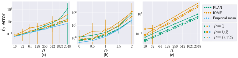
Figure 2. $\ell_{2}$ error for synthetic Gaussian data when varying (a) dimensions with data without a skew, (b) skewness of the variances, and (c) dimensions for skewed data — note that we compute error relative to the empirical mean rather than the statistical mean in this experiment as sampling error dominates in this setting. Also notice the different scales on the y-axis.

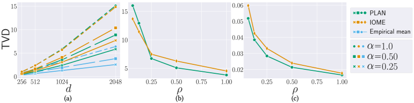
Figure 3. (a) Synthetic binary data, varying the ratio of 0s to 1s (b) Kosarak dataset (c) POS dataset

Name	$n$	$\rho$	$M$	$d$	$\boldsymbol{\sigma^{2}}$	$\boldsymbol{\mu}$
Gaussian A	$4000$	$\{1,0.5,0.125\}$	$\sqrt{50}d$	$\{16,32,\hbox to10.00002pt{.\hss.\hss.},2048\}$	$\left(1,\hbox to10.00002pt{.\hss.\hss.},1\right)$	$0^{d}$
Gaussian B	$10\,000$	$\{1,0.5,0.125\}$	$100d\max\left\{\boldsymbol{\sigma}\right\}$	$2048$	$\left(\left(\frac{d}{d}\right)^{\alpha},\left(\frac{d}{d-1}\right)^{\alpha},\hbox to10.00002pt{.\hss.\hss.},\left(\frac{d}{1}\right)^{\alpha}\right)$	$10^{d}$
Gaussian C	$10\,000$	$\{1,0.5,0.125\}$	$100d\max\left\{\boldsymbol{\sigma}\right\}$	$\{16,32,\hbox to10.00002pt{.\hss.\hss.},2048\}$	$\left(\left(\frac{d}{d}\right)^{2},\left(\frac{d}{d-1}\right)^{2},\hbox to10.00002pt{.\hss.\hss.},\left(\frac{d}{1}\right)^{2}\right)$	$10^{d}$
Binary	$4096$	$\{1,0.5,0.125\}$	$\|\boldsymbol{\hat{\sigma}^{2/3}}\|_{2}$	$\{256,512,\hbox to10.00002pt{.\hss.\hss.},2048\}$	$\sigma_{i}^{2}=\mu_{i}(1-\mu_{i})$	$\mu_{i}=\begin{cases}\tfrac{1}{2}&i\leq\alpha d\\ \tfrac{1}{100}&\text{else}\end{cases}$
Kosarak	$75\,462$	$\{1,0.5,0.25,0.125,0.0625\}$	$\|\boldsymbol{\hat{\sigma}^{2/3}}\|_{2}$	$27\,983$	Fixed dataset
POS	$515\,596$	$\{1,0.5,0.25,0.125,0.0625\}$	$\|\boldsymbol{\hat{\sigma}^{2/3}}\|_{2}$	$1\,657$	Fixed dataset
Global setting: $\rho_{1}=0.25\rho/d,\rho_{2}=0.25(\rho-\rho_{1}),\rho_{3}=\rho-\rho_{1}-\rho_{2}$.

Table 1. Settings for the experiments. All experiment settings run 50 times for each algorithm. iome is run with 20 steps for the binary quantile selection. Note that $\rho_{1}$ is split between recentering and variance prediction for plan.

To put plan’s utility into context, we measure error in diverse experimental settings. We use the empirical mean as a baseline, since it reflects an inevitable lower bound, i.e. the sampling error $\tilde{O}(\|\boldsymbol{\sigma}\|_{2}/\sqrt{n})$. Additionally we compare plan to Instance-optimal mean estimation (iome) (Huang et al., 2021), which has been shown to perform at least as good as CoinPress (Biswas et al., 2020) in empirical settings (Huang et al., 2021) hence representing the current state-of-the-art for differentially private mean estimation. Since plan works for $(\boldsymbol{\sigma},p)$-well concentrated distributions, we evaluate accuracy for Gaussian and binary data, representing $\ell_{2}$ and $\ell_{1}$ error, respectively. We run our experiments with synthetic data as input. For the binary case, we also evaluate our error on the Kosarak dataset (Benson et al., 2018) which represents user visits (or, conversely, non-visits) to webpages, as well as the Point of Sale (POS) dataset which represents user purchases.

7.1. Implementation

We evaluate the empirical accuracy of plan by instantiating Algorithm 1 in Python 3. Our implementation contains two different instantiations of plan: one version for binary data ($p=1$), and one version for data from multivariate Gaussian distributions ($p=2$). The pseudo code for both instantiations of plan is shown in LABEL:code:plan. Both instances use the PrivQuantile search by Kaplan et al. (2022). The implementation of iome uses the original source code from Huang et al. (2021).

⬇

1def PLAN(data, n, d, M, p, rho, beta) {

2 rho1, rho2, rho3 = divideBudget(rho)

3 mu = center(M, rho1*0.25, data, beta/3)

4 std = estimateStd(M, rho1*0.75, data, beta/3)

5 scaleFactors = std**(-1/(p + 2))

6 y = (data-mu) * scaleFactors #coordinate-wise

7 k = sqrt(n) + rankError(M, n, d, rho2, beta/3)

8 z = clip(M, y, rho2, (n-k)/n)

9 return ((z+noise(p, rho3))/scaleFactors)+mu

10}

Listing 1: Pseudo code for the plan instantiation for $n$ vectors in $\mathbb{R}^{d}$, with each coordinate being in the range ${[-M,M]}$, targeting the expected $\ell_{p}$ error with privacy budget $\rho$ and a failure probability of at most $\beta$. Note that budget is spent on estimating the standard deviation unlike in Algorithm 1 where $\boldsymbol{\hat{\sigma}^{2}}$ is an input parameter.

Estimating $\boldsymbol{\sigma}^{2}$.

Note that Algorithm 1 assumes an estimate of the variances as input. In the absence of public knowledge, these parameters have to be estimated on the actual data in a differentially private way, as mentioned in LABEL:code:plan.

In the Gaussian case, given $X,Y\sim\mathcal{N}({\mu_{i}},\sigma_{i}^{2})$, $\mathbf{E}[(X-Y)^{2}/2]=\mathbf{E}[X^{2}]-\mathbf{E}[X]^{2}=\sigma_{i}^{2}$. Since $(X-Y)^{2}/2$ follows a generalized Chi-squared distribution, we use PrivQuantile for each coordinate to differentially privately estimate the median $\tilde{\mu}_{i}$ of a sequence of values $(X-Y)^{2}/2$, and estimate the mean as $\tilde{\mu_{i}}/(9/7)^{3}$. In the binary case where each coordinate is 1 with probability $q_{i}$, we estimate the variance by private estimation of the mean $\tilde{q}_{i}$ using the Gaussian mechanism with $\ell_{2}$-sensitivity $1/n$, and use ${\hat{\sigma}}^{2}_{i}=\tilde{q}_{i}(1-\tilde{q}_{i})$. In both cases, we regularize the estimate $\boldsymbol{\hat{\sigma}}$ on the standard deviation by adding $\|\boldsymbol{\hat{\sigma}}\|_{1}/d$ to each coordinate.

In Appendix D, we generalize the estimator on Gaussian data to distributions with bounded fourth moment and provide more details on the empirical evaluation.

Bounding the clipping universe.

Having an estimate on $\boldsymbol{\sigma}^{2}$ provides an opportunity to trim the universe used when searching for the clipping radius (Algorithm 1 6). Specifically, instead of using $M\sqrt{d}$ as the upper bound to cover the entire universe, we use the tighter bound $\sqrt{\log(d)\log(1/\beta)\|\boldsymbol{\sigma}\|_{1}}$.

7.2. Experiment design

Parameter input space.

The following parameters needs to be chosen for each execution of plan: the universe $M$, the $\ell_{p}$ error norm, and the privacy budget $\rho$ as well as the partitioning of $\rho$ into $\rho_{1},\rho_{2},\rho_{3}$. Since iome uses a binary search for their quantile selection, the amount of steps to use also needs to be chosen. iome sets the amount of steps to 10 by default, but an empirical investigation shows that this value is too low for many of our settings — the binary quantile search ends early which causes inaccurate results. To level the playing field, we use 20 steps to ensure that iome does not suffer any disadvantages from the binary quantile search failing.

Input data.

We will use both synthetic, and real world datasets to evaluate plan. When generating synthetic data, the following parameters need to be chosen: the dataset size $n$, the dimensionality $d$, the means $\boldsymbol{\mu}$, and the variances $\boldsymbol{\sigma^{2}}$. Since plan and iome both ignore potential correlations in data, we use covariance matrices of the form $\Sigma=\text{diag}(\boldsymbol{\sigma}^{2})$.

7.2.1. Gaussian data

To show the effectiveness of plan on Gaussian data, we design three diverse experiments. The first experiment (Gaussian A) reflects the parameter settings used in previous work by Huang et al. (2021) where data has no skew, which is the case iome is intended for. The second experiment (Gaussian B) simulates data ranging from no to significant skew across dimensions, showcasing how plan improves with increasing skew. Finally, the third experiment (Gaussian C) highlights how plan scales as dimensionality increases for data with a skew. For each experiment, we vary $\rho$ between $1$ and $0.125$ to show how accuracy scales in higher and lower privacy regimes. We summarize the settings used in the experiments in Table 1.

Budget division.

Our algorithm needs to perform two preprocessing steps: estimating $\boldsymbol{\mu}$ for re-centering, and estimating $\boldsymbol{\sigma^{2}}$ for scaling the noise. We fix the initial estimation of $\boldsymbol{\mu}$ and $\boldsymbol{\sigma^{2}}$ to use 25% of the total privacy budget — the same proportion used for preprocessing as in Huang et al. (2021). In the same spirit, we set the budget to determine the clipping threshold ($\rho_{2}$) to 25% of the remaining budget, and use the larger part ($\rho_{3}$) for the Gaussian noise.

Choosing valid settings.

Just like for iome, $M$ needs to be set such that $\boldsymbol{\mu}$ is within the universe. We will use two different approaches to set $M$: the approach from (Huang et al., 2021) ($M=\sqrt{50}d$), and a more pessimistic approach where we assume all values have the worst case standard deviation across all dimensions, and create more leeway by scaling with a constant ($M=100d\max\left\{\boldsymbol{\sigma}\right\}$).

Additionally, the rank error needs to be tuned such that PrivQuantile search can be expected to return a quantile close to the requested one. Since plan calls PrivQuantile multiple times, plan needs to tolerate the worst case rank error for all calls. We set $n$ such that the rank error is at most $0.1n$ for each value of $\rho$.

Gaussian A: no skew. To show that plan performs comparatively to iome we run it on data where variance is the same across all dimensions. In this setting we expect plan to perform similar to iome. We reuse the experiment settings used by Huang et al. (2021) for a fair comparison.

Gaussian B: varying skewness. To show how plan improves as the input data’s skew increases, we vary the skewness of the variance. We introduce a parameter $\alpha$, and simulate a Zipfian like skew to the data and set the variances $\boldsymbol{\sigma^{2}}=((d/d)^{\alpha},(d/(d-1))^{\alpha},\hbox to10.00002pt{.\hss.\hss.},(d/1)^{\alpha})$ for $\alpha\in\{0,0.5,\hbox to10.00002pt{.\hss.\hss.},2\}$. In this setting we expect plan to outperform iome for $\alpha>0$.

Gaussian C: varying dimensionality. To show how plan’s advantage scales compared to iome, we vary dimensionality as we expect an improvement up to a factor $\sqrt{d}$. Since plan’s advantage is based on data having a skew, we set $\boldsymbol{\sigma^{2}}=(d/d)^{\alpha},(d/(d-1))^{\alpha},\hbox to10.00002pt{.\hss.\hss.},(d/1)^{\alpha}$, where $\alpha=2$. Note that plan’s improvement is in noise error, as sampling error is unavoidable — we compute the error relative to the empirical mean in this experiment to showcase the difference in noise error.

7.2.2. Binary data

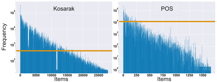
Figure 4. Histogram for Kosarak (left) and POS (right). The orange line is the smallest allowed variance according to Lemma 5.3 which we clip to.

To diversify our experimental scope, we consider binary data represented by $n$ bitvectors of length $d$ in which each bit $i,1\leq i\leq d,$ is set independently to 1 with probability $q_{i}$. We usually think about these bitvectors as sets representing a selection of items from $\{1,\ldots,d\}$. To vary the error measure, we focus on the $\ell_{1}$ error. This is akin to computing the total variation distance (TVD) $1/2\|x-y\|_{1}$, but we avoid the normalization of $x$ and $y$ to have unit $\ell_{1}$ norm.

We design three experiments: the first (Binary) varies the skewness in the probabilities to make controlled experiments on the accuracy of plan. The two remaining experiments (Kosarak, POS) use real world datasets that naturally exhibit skew between coordinates.

Binary: Varying skewness. This experiment follows the same design principle as Gaussian B: to show how skewness affects the performance of plan. Given $n,d,$ and $\rho$, we choose two probabilities $q_{1}=0.5$ (high variance) and $q_{2}=0.01$ (low variance). Given $\alpha\in[0,1]$, we sample the first $\lceil\alpha d\rceil$ bits with probability $q_{1}$ each, and the remaining positions with probability $q_{2}$. The low variance setting is slightly below the minimum threshold of $1/d^{2/5}$ discussed in Lemma 5.3 to test the robustness of our implementation. We clip all estimated variances to $1/d^{2/5}$ from below.

Kosarak: Website visits. The Kosarak dataset represents click-stream data of a Hungarian news portal. There are $n=75\,462$ users and a collection of $d=27\,983$ websites. In total, users clicked on 4 194 414 websites (each user clicked on 55.6 websites on average), and there is a large skew between the websites, see Figure 4.

POS: Shopping baskets. The POS dataset contains merchant transactions on $d=1\,657$ categories from $n=515\,596$ users. In total, there are $3\,367\,019$ transactions (around 6.5 on average per user). Again, there is large skew in the different categories, see Figure 4. The dataset is particularly challenging because the minimum variance $d^{-2/5}$ (cf. Lemma 5.3) has to be clipped on many coordinates.

7.3. Results

For the Gaussian case, we ran our experiments using Python 3.11.3 on a MacBook Pro with 24GB RAM, and the Apple M2 chip (8-core CPU). For the binary case, we had to run the experiments on a more powerful machine to support iome on the real world datasets. While Kosarak and POS are sparse datasets, iome requires that the entire dataset (not just the sparse representation) is loaded into memory to perform a random rotation the algorithm uses as a preprocessing step. As a consequence, we ran the binary experiments using Python 3.6.9 on a machine with 512GB RAM, on a Intel(R) Xeon(R) CPU E5-2690 v4 @ 2.60GHz (56-core CPU). Even on this more powerful machine, a single run of iome took at least 26 minutes on Kosarak, and at least 9 minutes on POS. In comparison, plan spent an average of 12, and 9 seconds running on Kosarak and POS, respectively.

7.3.1. Gaussian data

All results are shown in Figure 2. Figure 2 (a) shows Gaussian A, where plan and iome have comparable accuracy until $d=2048$, when plan performs worse as we reach a setting where the assumptions on rank error no longer hold. This is expected behavior as plan spends some additional budget estimating $\boldsymbol{\sigma}^{2}$ in comparison to iome.

Figure 2 (b) shows Gaussian B, where plan performs better than iome for $\alpha>0$. For $\alpha=0$ the error between plan and iome is similar. This is expected behavior, as $\alpha=0$ represents the same input data as in Gaussian A. Notice how plan approaches the empirical mean as $\alpha$ grows for both $\rho=0.5$ and $\rho=1$.

Figure 2 (c) shows Gaussian C, where we compare against the empirical mean since sampling error is larger than the noise error for plan in this case. As expected, plan increases its advantage over iome as $d$ grows.

7.3.2. Binary data

All results are shown in Figure 3. Figure 3 (a) shows Binary, where plan has an advantage over iome for $\alpha<1$ which increases as $\alpha$ decreases. This is the expected behavior, as plan is able to exploit the skew in variance whereas iome treats every dimension the same.

Figure 3 (b) shows Kosarak. As we can see, plan outperforms iome for sufficiently large values of $\rho$. For small $\rho$ ($\rho\leq 0.125$), plan is running in a invalid setting — our assumptions on rank error are not fulfilled in these cases.

Figure 3 (c) shows POS. plan has a slight advantage compared to Instance-optimal mean estimation in this case, which decreases as $\rho$ grows.

8. Related Work

Our work builds on concepts from multiple areas within the literature on differential privacy. We provide an overview of the most closely related work.

Statistical private mean estimation.

There is a large, recent literature on statistical estimation for $d$-dimensional distributions under differential privacy, mainly focusing on the case of Gaussian or subgaussian distributions (Alabi et al., 2022; Ashtiani and Liaw, 2022; Biswas et al., 2020; Brown et al., 2021, 2023; Du et al., 2020; Duchi et al., 2023; Hopkins et al., 2022; Karwa and Vadhan, 2018; Kamath et al., 2019, 2022; Kothari et al., 2022). The error on mean estimates is generally expressed in terms of Mahalanobis distance, which is natural if we want the error to be preserved under affine transformations. Some of these efficient estimators are even robust against adversarial changes to the input data (Alabi et al., 2022; Kothari et al., 2022). Others estimators work even for rather heavy-tailed distributions (Kamath et al., 2020). What all these estimators have in common is that the nominal dimension $d$ influences the privacy-utility trade-off such that higher-dimensional vectors have a worse trade-off. To our best knowledge, the algorithm among these that has been shown to work best in practical (non-adversarial) settings is the CoinPress algorithm of Biswas et al. (2020).

Adapting to the data.

The best private mean estimation algorithms are near-optimal for worst-case $d$-dimensional distributions in view of known lower bounds (Cai et al., 2021). However, it is natural to consider ways of improving the privacy-utility trade-off whenever the input distribution has some structure. One way of going beyond the worst case is by privately identifying low-dimensional structure (Amin et al., 2019; Dwork et al., 2014; Hardt and Price, 2014; Singhal and Steinke, 2021). Such methods effectively reduce the mean estimation problem to an equivalent problem with a dimension smaller than $d$. However, we are not aware of any work showing this approach to be practically relevant for mean estimation.

Another approach for adapting to the data is instance optimality, introduced by Asi and Duchi (2020) and studied in the context of mean estimation by Huang et al. (2021) who use $\ell_{2}$ error (or mean square error) as the utility metric. The goal is optimality, i.e. matching lower bounds, for a class of inputs with a given diameter but no further structure. Huang et al. (2021) found that their private mean estimation algorithm often has smaller error than CoinPress in practice. Because of this, and since they also aim to minimize an $\ell_{p}$ error, this algorithm was chosen as our main point of comparison.

Neither of the mentioned approaches take skew in the data distribution into account, so we believe this is a novel aspect of our work in the context of mean estimation. However, we mention that privacy budgeting in skewed settings has recently been studied in the context of multi-task learning Krichene et al. (2023). Also, the related setting of mean estimation with heterogeneous data (where the sensitivity with respect to different client’s data can differ) was recently studied by Cummings et al. (2022).

Clipping.

An important aspect of private mean estimation for unbounded distributions, in theory and practice, is how to perform clipping to reduce the sensitivity. This has in particular been studied in the context of differentially private stochastic gradient descent (McMahan et al., 2018; Pichapati et al., 2019; Andrew et al., 2021; Bu et al., 2022). Though clipping introduces bias, Kamath et al. (2023) have show that this is unavoidable without additional assumptions.

Huang et al. (2021) used a clipping method designed to cut off a carefully chosen, small fraction of the data points. The clipping done in plan follows the same pattern, though it is applied only after carefully scaling data according to the coordinate variances. Thus, it corresponds to clipping to an axis-aligned ellipsoid.

To formally bound clipping error one can either express the error in terms of the diameter of the dataset or analyze the error under some assumption on the data distribution. Both approaches are explored in Huang et al. (2021), but in this paper we have chosen to focus on the latter.

9. Conclusion and future work

We introduce Private Limit Adapted Noise (plan), a family of algorithms for differentially private mean estimation of $d$-dimensional data. plan exploits skew in data’s variance to achieve better $\ell_{p}$ error. In the case of $\ell_{2}$ error we achieve a particularly clean bound, namely error proportional to $\|\boldsymbol{\sigma}\|_{1}$. This is never worse than the error of $\sqrt{d}\|\boldsymbol{\sigma}\|_{2}$ obtained by previous methods and gives an improvement up to a factor of up to $\sqrt{d}$ when $\boldsymbol{\sigma}$ is skewed. While the privacy guarantees hold for any input, the error bounds hold for independently sampled data from distributions that follow a well-defined assumption on concentration.

Finally, we implement two plan instantiations and empirically evaluate their utility. Practice follows theory — plan outperforms the current state-of-the-art for skewed datasets, and is able to perform competitively for datasets without skewed variance. To aid practitioners in implementing their own plan, we summarize some practical advice based on our lessons learned.

Advice for practitioners.

When implementing a plan instantiation, practitioners should pose the following questions:

1. Is there a suitable estimator for the variances ${\sigma}_{i}^{2}$ of the data distribution?

2. Can a tighter bound on the clipping universe ($M\sqrt{d}$) be used?

3. How robust is plan for my given settings, i.e., will the rank error be too high and cause plan to fail?

We give examples of how to answers these question in our evaluation. To answer Question 1, we derive private variance estimators tuned to the data distribution. As for Question 2, when the distribution is $(\boldsymbol{\sigma},p)$-well concentrated, much better bounds on the universe size can be derived by using Assumption (5) in Definition 4.4. Finally, answering Question 3, robustness must carefully be evaluated using the assumption on minimum $\rho$ values and maximum dimensionality $d$. Both parameters in conjunction give minimum requirements to the required sample size $n$.

Future work.

We conclude with some possible future directions.

• An interesting avenue to explore would be to capture skew in the input vectors that is not necessarily visible in the standard basis. For example, one could use private PCA to rotate the space into a basis in which coordinates are nearly independent, and then apply plan.

• Though our algorithm chooses optimal parameters within a class of mechanisms, we have not ruled out that an entirely different approach could have better performance. We conjecture that for any choice of $\boldsymbol{\sigma}$ there exist an input distributions for which our mechanism achieves an optimal trade-off up to logarithmic factors.

• Finally, we rely on having access to reasonable estimates of coordinate variances (the diagonal of the covariance matrix). It would be interesting to study this problem in its own right, since it is likely that estimating the entire covariance matrix is strictly harder.

Appendix A Useful statements from probability theory

Lemma A.1 (Bernstein’s inequality).

Let $X_{1},\ldots,X_{n}$ be independent zero-mean random variables. Suppose that $|X_{i}|\leq M$ almost surely for all $i$. Then for all $t>0$,

$$\Pr\left[\sum_{i=1}^{n}X_{i}\geq t\right]\leq\exp\left(-\frac{t^{2}/2}{\sum_{i=1}^{n}\mathbf{E}[X_{i}^{2}]+Mt/3}\right).$$

Lemma A.2 ((Winkelbauer, 2012, Equation (18))).

The $p$th absolute moment of a zero-centered Gaussian distribution for any $p>0$ is

$$\mathbf{E}\left[\left|\mathcal{N}\left(0,\sigma^{2}\right)\right|^{p}\right]=\sigma^{p}\cdot\frac{2^{p/2}\Gamma\left(\tfrac{p+1}{2}\right)}{\sqrt{\pi}}.$$

Lemma A.3 (Generalized Chernoff-Hoeffding Bound (Dubhashi and Panconesi, 2009)).

Let $X:=\sum_{1\leq i\leq n}X_{i}$ where $X_{i},1\leq i\leq n$ are independently distributed in $[a_{i},b_{i}]$ for $a_{i},b_{i}\in\mathbf{R}$. Then for all $t>0$

$$\Pr[|X-\mathbf{E}[X]|\geq t]\leq 2\exp\left(\frac{-t^{2}/2}{\sum_{i}\left(a_{i}-b_{i}\right)^{2}}\right).$$

Appendix B Proof of Theorem 4.5

Theorem B.1.

For sufficiently large $n=\tilde{\Omega}(\max(\sqrt{d/\rho},\rho^{-1}))$, plan with parameters $k=\sqrt{n}$ and $\rho_{1}=\rho_{2}=\rho_{3}=\rho/3$ is $\rho$-zCDP. If inputs are independently sampled from a $(\boldsymbol{\sigma},p)$-well concentrated distribution, the mean estimate has expected $\ell_{p}$ error

$$\tilde{O}\left(1+\frac{||\boldsymbol{\sigma}||_{p}}{\sqrt{n}}+\frac{\|\boldsymbol{\sigma}\|_{2p/(p+2)}}{n\sqrt{\rho}}\right)$$

with probability at least $1-\beta$, where $\tilde{O}$ suppresses polylogarithmic dependencies on $1/\beta$, $n$, $d$, and the bound $M$ on the $\ell_{\infty}$ norm of inputs.

Proof.

We proceed in the same three steps as in the proof of Theorem 4.3 in Section 4.

By Lemma 4.2, with probability at least $1-\beta$, all $|{\mu}_{i}-{\tilde{\mu}}_{i}|\leq{\sigma}_{i}$. In this case, $\|\boldsymbol{\mu}-\boldsymbol{\tilde{\mu}}\|_{p}=O(\|\boldsymbol{\sigma}\|_{p})$.

Let $J=\{j\in\{1,\dots,n\}\;|\;\|\boldsymbol{y}^{(j)}\|_{2}>C\}$ denote the set of indices of vectors affected by clipping in plan. By the triangle inequality and assuming the bound of part 1 holds,

$$\sum_{j\in J}\left\|(\boldsymbol{x}^{(j)}-\boldsymbol{\tilde{\mu}})\right\|_{p} \leq\sum_{j\in J}\left\|(\boldsymbol{x}^{(j)}-\boldsymbol{\mu})\right\|_{p}+|J|\cdot\left\|\boldsymbol{\mu}-\boldsymbol{\tilde{\mu}}\right\|_{p}$$

$$\leq\sum_{j\in J}\left\|(\boldsymbol{x}^{(j)}-\boldsymbol{\mu})\right\|_{p}+2|J|\cdot\|\boldsymbol{\sigma}\|_{p}\enspace.$$

By assumption (4) the probability that $\|\boldsymbol{x}^{(j)}-\boldsymbol{\mu}\|_{p}^{p}>t\|\boldsymbol{\sigma}\|_{p}^{p}$ is exponentially decreasing in $t$, so setting $t=\tilde{\Omega}(\log^{p}(n/\beta))$ we have $\|\boldsymbol{x}^{(j)}-\boldsymbol{\mu}\|_{p}=\tilde{O}(\|\boldsymbol{\sigma}\|_{p})$ for all $j=1,\dots,n$ with probability at least $1-\beta$. Using the triangle inequality again we can now bound

$$\sum_{j\in J}\|\boldsymbol{x}^{(j)}-\boldsymbol{\mu}\|_{p}=\tilde{O}(|J|\cdot\|\boldsymbol{\sigma}\|_{p})\enspace.$$

The same line of argument as in Section 4.3 shows that $|J|=\tilde{O}(k+\sqrt{1/\rho})$. Thus, the clipping error can be bounded by $O((k+\sqrt{1/\rho})\|\boldsymbol{\sigma}\|_{p})$, and setting $k=n^{-1/2}$ balances the clipping error with the sampling error $\frac{\|\boldsymbol{\sigma}\|_{p}}{\sqrt{n}}$.

Lastly, we consider the error due to noise. First, we find a bound on the clipping threshold $C$. By the triangle inequality, we may bound

$$\|\boldsymbol{y}^{(j)}\|_{2} =\left\|(\boldsymbol{x}^{(j)}-\boldsymbol{\tilde{\mu}})\,\hat{\Sigma}^{-\tfrac{1}{p+2}}\right\|_{2}$$

$$\leq\left\|(\boldsymbol{x}^{(j)}-\boldsymbol{\mu})\,\hat{\Sigma}^{-\tfrac{1}{p+2}}\right\|_{2}+\left\|(\boldsymbol{\mu}-\boldsymbol{\tilde{\mu}})\,\hat{\Sigma}^{-\tfrac{1}{p+2}}\right\|_{2}$$

The $i$th coordinate of the first vector $(\boldsymbol{x}^{(j)}-\boldsymbol{\mu})\,\hat{\Sigma}^{-1/(p+2)}$ equals $({x}^{(j)}_{i}-{\mu}_{i})/{{\hat{\sigma}}_{i}}^{2/(p+2)}$, so assumption (5) implies that the length of the first vector is $\tilde{O}(\sqrt{\|\boldsymbol{\sigma}^{2p/(p+2)}\|_{1}})$ with high probability. By using that the $i$th coordinate of $|\boldsymbol{\mu}-\boldsymbol{\tilde{\mu}}|\leq\boldsymbol{\sigma}$, $(\boldsymbol{\mu}-\boldsymbol{\tilde{\mu}})\,\hat{\Sigma}^{-1/(p+2)}$ has absolute value $\tilde{O}(\sqrt{\|\boldsymbol{\sigma}^{2p/(p+2)}\|_{1}})$ as well. The clipping value of $C$ is bounded by the maximum length of a vector $\|\boldsymbol{y}^{(j)}\|_{2}$, and thus $C^{2}=\tilde{O}(\|\boldsymbol{\sigma}^{2p/(p+2)}\|_{1})$, with probability at least $1-\beta$.

The scaled noise vector $\boldsymbol{\eta}\,\hat{\Sigma}^{1/(p+2)}$ has distribution $\mathcal{N}(\boldsymbol{0},\frac{2C^{2}}{\rho_{3}}\hat{\Sigma}^{2/(p+2)})$. Using ${\hat{\sigma}}_{i}<\left({\sigma}_{i}^{\frac{2p}{p+2}}+\|\boldsymbol{\sigma}^{\frac{2p}{p+2}}\|_{1}/d\right)^{\frac{p+2}{2p}}$ and Lemma A.2, we conclude

$$\mathbf{E}[\|\boldsymbol{\eta}\,\hat{\Sigma}^{1/(p+2)}\|_{p}^{p}] =O\left(\tfrac{2^{p}C^{p}}{\rho_{3}^{p/2}}\sum_{i=1}^{d}\hat{\Sigma}_{ii}^{p/(p+2)}\right)$$

$$=O\left(\tfrac{2^{p}C^{p}}{\rho_{3}^{p/2}}\sum_{i=1}^{d}\hat{{\sigma}}_{i}^{2p/(p+2)}\right)$$

$$=\tilde{O}\left(\frac{2^{p}\|\boldsymbol{\sigma}\|_{2p/(p+2)}^{p}}{\rho_{3}^{p/2}}\right)\enspace.$$

The result of Theorem 4.5 is achieved by putting together the different error terms as in the proof of Theorem 4.3.

∎

Appendix C Choosing The Scaling Value

Here we discuss the choice of scaling of plan. For parameters $p$ and $\boldsymbol{\hat{\sigma}}\in\mathbf{R}^{d}$ we scale each coordinate $i$ by $\boldsymbol{\sigma}^{-2/(p+2)}$ on 4. When returning the mean estimate on 5 each coordinate $i$ is scaled back by $\boldsymbol{\sigma}^{2/(p+2)}$. The choice of scaling affects how noise is distributed across coordinates. In this section we consider a simpler setting with independent queries with known sensitivities where we restrict ourselves to adding noise such that there is no clipping error. We choose the scaling parameters that minimizes the $p$th moment of the noise.

Consider the problem of privately answering $d$ independent real-valued queries with different sensitivities. We denote the sensitivity of the $i$th query as ${\Delta}_{i}$ and the vector of all sensitivities as $\boldsymbol{\Delta}$. We want to minimize the $p$th moment of the noise. That is, let $\boldsymbol{\eta}\in\mathbf{R}^{d}$ denote the vector where $\boldsymbol{\eta}_{i}$ is the value of the noise added to the $i$th query. We want to minimize $\mathbf{E}[\|\boldsymbol{\eta}\|_{p}^{p}]$. As discussed in section 1, standard approaches either adds a lot of noise for queries with low or high sensitivity as we show here. We can think of the queries as a $d$-dimensional query which we can release by adding noise from $\mathcal{N}(\boldsymbol{0},\frac{\bar{\Delta}^{2}}{2\rho}\mathbf{I})$ where the sensitivity is $\bar{\Delta}=\sqrt{\sum_{i\in[d]}{\Delta}_{i}^{2}}=\|\boldsymbol{\Delta}\|_{2}$. This approach adds noise of the same magnitude to each coordinate which might be excessive for queries with very low sensitivity. The privacy budget is effectively split up between queries weighted linearly by $\boldsymbol{\Delta}$. Alternatively we could split the privacy budget evenly and answer each query independently by adding noise from $\mathcal{N}(\boldsymbol{0},d\cdot\frac{\bar{\Delta}_{i}^{2}}{2\rho})$. This approach is equivalent to first scaling each coordinate by ${\Delta}_{i}^{-1}$ and scale back after adding noise from $\mathcal{N}(\boldsymbol{0},\frac{d}{2\rho}\mathbf{I})$. However, this approach adds too much noise to coordinates with high sensitivity. We want to balance the two approaches and as such plan uses an in-between scaling value. We can think of our approach as allocating more privacy budget for queries with high sensitivity, but not so much that it creates large errors for queries with low sensitivity.

Let $\boldsymbol{x}\in\mathbf{R}^{d}$ be the answer to the $d$ queries and let $\boldsymbol{s}\in\mathbf{R}^{d}$ be a scaling vector. Let $\boldsymbol{y}=\boldsymbol{x}S^{-1}$ denote the scaled down answers where $S$ is a diagonal matrix with $\boldsymbol{s}$ on the diagonal. We can privately release $\boldsymbol{y}$ by adding noise from $\mathcal{N}(\boldsymbol{0},\frac{\bar{\Delta}^{2}}{2\rho}\mathbf{I})$ where $\bar{\Delta}^{2}=\sum_{i\in[d]}{\Delta}_{i}^{2}/s_{i}^{2}$. When scaling back we multiply the noisy answers with $S$. Our goal is to minimize the $p$th moment. Specifically, we want to choose $\boldsymbol{s}$ to minimize

$$\mathbf{E}\left[\|\mathcal{N}(\boldsymbol{0},\frac{\bar{\Delta}^{2}}{2\rho}\mathbf{I})S\|_{p}^{p}\right]\enspace,$$

where $\bar{\Delta}$ and $S$ are defined as above.

Lemma C.1.

The $p$th moment of the algorithm above is

$$\mathbf{E}\left[\|\mathcal{N}(\boldsymbol{0},\frac{\bar{\Delta}^{2}}{2\rho}S^{2})\|_{p}^{p}\right]=\frac{\Gamma\left(\frac{p+1}{2}\right)}{\rho^{p/2}\sqrt{\pi}}\sum_{i\in[d]}(\bar{\Delta}\cdot\boldsymbol{s}_{i})^{p}$$

Proof.

It follows from linearity of expectation by summing over each coordinate. By Lemma A.2 we have

$$\mathbf{E}\left[|\mathcal{N}(\boldsymbol{0},\frac{\bar{\Delta}^{2}}{2\rho}s_{i})|^{p}\right] =\left(\frac{\bar{\Delta}^{2}}{2\rho}s_{i}^{2}\right)^{p/2}\frac{2^{p/2}\Gamma\left(\frac{p+1}{2}\right)}{\sqrt{\pi}}$$

$$=\frac{\Gamma\left(\frac{p+1}{2}\right)}{\rho^{p/2}\sqrt{\pi}}(\bar{\Delta}\cdot s_{i})^{p}$$

∎

Since the fraction outside the sum is not affected by our choice of $\boldsymbol{s}$ we just have to find $\boldsymbol{s}$ that minimizes $\sum_{i\in[d]}(\bar{\Delta}\cdot s_{i})^{p}$.

Lemma C.2.

The $p$th moment of the noise is minimized for

$$s_{i}\propto{\Delta}_{i}^{2/(p+2)}.$$

Proof.

First notice that multiplying all entries in $\boldsymbol{s}$ by the same scalar does not change the result since the magnitude of noise added to $y$ would be scaled by the inverse of the scalar. As such, we can restrict our search to $\boldsymbol{s}$ such that $\bar{\Delta}^{2}=\sum_{i\in[d]}({\Delta}_{i}/s_{i})^{2}=1$. We also restrict our search to $\boldsymbol{s}$ with no negative values since negative values would simply fix the input and has no impact on the sensitivity. We use the method of Lagrange multipliers to find $\boldsymbol{s}$. The method is used to find local maxima or minima of a function subject to equality constraints. In our case, it turns our that there is only one minimum which means it is the global minimum. We want to minimize $\sum_{i\in[d]}s_{i}^{p}$ subject to the restriction $\sum_{i\in[d]}({\Delta}_{i}/s_{i})^{2}-1=0$. The minimum is at the stationary point of the Lagrangian function

$$\mathcal{L}(\boldsymbol{s},\lambda)=\sum_{i\in[d]}s_{i}^{p}+\lambda\left(\sum_{i\in[d]}({\Delta}_{i}/s_{i})^{2}-1\right),$$

where $\lambda\in\mathbf{R}$ is the Lagrange multiplier.

We start by finding the partial derivative of the Lagrangian function with respect to $s_{i}$.

$$\frac{\partial}{\partial s_{i}}\mathcal{L}(\boldsymbol{s},\lambda)=\frac{\partial}{\partial s_{i}}\boldsymbol{s}_{i}^{p}+\lambda(\Delta_{i}/\boldsymbol{s}_{i})^{2}=ps_{i}^{p-1}-2\lambda{\Delta}_{i}^{2}/s_{i}^{3}\enspace.$$

We then find the root of this function with respect to $s_{i}$, that is,

$$ps_{i}^{p-1}-2\lambda{\Delta}_{i}^{2}/s_{i}^{3} =0$$

$$s_{i}^{p+2} =2\lambda{\Delta}_{i}^{2}/p$$

$$s_{i} ={\Delta}_{i}^{2/(p+2)}\cdot\gamma\enspace,$$

where $\gamma=(2\lambda/p)^{1/(p+2)}$ is a scalar. This finishes the proof. ∎

Lemma C.3.

Let $\boldsymbol{s}\in\mathbf{R}^{d}$ be defined as in Lemma C.2. Then the $p$th moment of the mechanism described in this section is

$$\mathbf{E}\left[\|\mathcal{N}(\boldsymbol{0},\frac{\bar{\Delta}^{2}}{2\rho}\mathbf{I})S\|_{p}^{p}\right]=\frac{\Gamma\left(\frac{p+1}{2}\right)}{\rho^{p/2}\sqrt{\pi}}\|\boldsymbol{\Delta}\|_{2p/(p+2)}^{p}$$

Proof.

From Lemma C.1 we know that the above equality holds if $\sum_{i\in[d]}(\bar{\Delta}/s_{i})^{p}=\|\boldsymbol{\Delta}\|_{2p/(p+2)}^{p}$. Continuing the calculations from the proof of the previous Lemma we see that for $\bar{\Delta}=1$ we have

$$\sum_{i\in[d]}({\Delta}_{i}/s_{i})^{2} =\bar{\Delta}$$

$$\frac{1}{\gamma^{2}}\sum_{i\in[d]}{\Delta}_{i}^{2p/(p+2)} =1$$

$$\gamma =\sqrt{\sum_{i\in[d]}{\Delta}_{i}^{2p/(p+2)}}$$

Finally, we find that the $p$th moment is proportional to

$$\sum_{i\in[d]}(s_{i})^{p} =\sum_{i\in[d]}\left({\Delta}_{i}^{2/(p+2)}\sqrt{\sum_{i\in[d]}{\Delta}_{i}^{2p/(p+2)}}\right)^{p}$$

$$=\left(\sum_{i\in[d]}{\Delta}_{i}^{2p/(p+2)}\right)^{p/2}\sum_{i\in[d]}{\Delta}_{i}^{2p/(p+2)}$$

$$=\left(\sum_{i\in[d]}{\Delta}_{i}^{2p/(p+2)}\right)^{1+p/2}=\|\boldsymbol{\Delta}\|_{2p/(p+2)}^{p}\enspace.$$

∎

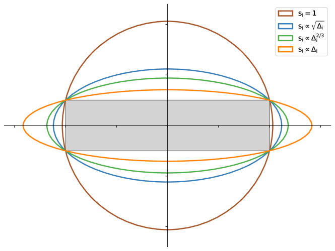
Figure 5. Shape of noise for different scaling parameters.

Figure 5 shows an example of this scaling in two dimensions, where the sensitivity of one query is 4 times as high as the other. The green and blue lines show the shape of noise when optimizing for the first and second moment, respectively. In both cases we use most of the privacy budget for the horizontal axis which allows us to add less noise than the orange line where the budget is split evenly. But we are still able to add less noise to the vertical axis as opposed to the brown line without scaling.

We use the scaling as described above for plan. However, in our setting we do not use sensitivities of queries. Instead we scale each coordinate based on the estimate of the standard deviation. The intuition is the same: we spend more privacy budget on coordinates with high standard deviation but we still add less noise to coordinates with low standard deviation.

Appendix D Algorithms for Variance Estimation

While plan (Algorithm 1) assumes that estimates on the standard deviations are known, such estimates have to be computed in a differentially private manner. Two such ways were described in Section 7 and we will provide more details and empirical results in this section.

We remark that the standard attempt to estimate the variance from a mean estimate $\tilde{\mu}$ is

$$\left(1/n\sum_{i=1}^{n}{x_{i}^{2}}\right)-\tilde{\mu}^{2}$$

If $x_{i}\in[-M,M]$, the sensitivity of this function is $M^{2}/n$, which, depending on the application, means that too much noise must be added.

D.1. A Generic Variance Estimation Algorithm

Algorithm 2 VarianceEstimate

1:Input: Samples $x^{(1)},\dots,x^{(n)}\in\mathbf{R}$ from $\mathcal{D}$

2:Parameters: $M,\rho,k$

3:Split $x^{(1)},\ldots,x^{(n)}$ into $n^{\prime}=\lfloor\tfrac{n}{2k}\rfloor$ groups $G_{1},\ldots,G_{n^{\prime}}$.

4:For each $i\in\{1,\ldots,n^{\prime}\}$: For $G_{i}=(\hat{x}_{i}^{(1)},\ldots,\hat{x}_{i}^{(2k)})$, let $\hat{y}^{(i)}=\sum_{j=1}^{k}(\hat{x}_{i}^{(2j)}-\hat{x}_{i}^{(2j+1)})^{2}/2$.

5:return $\tilde{\sigma}^{2}\leftarrow\frac{\textsc{PrivQuantile}_{\rho}^{M}(\hat{y}^{(1)},\dots,\hat{y}^{(n^{\prime})},1/2)}{k}.$

Given a distribution $\mathcal{D}$ with mean $\mu$ and variance $\sigma^{2}$, we showed in Section 7 that for $X,Y\sim\mathcal{D}$, $\mathbf{E}\left[(X-Y)^{2}/2\right]=\sigma^{2}$. Algorithm 2 is a generalization of the approach used for Gaussian in Section 7. For Gaussian data, we made use of the fact that $(X-Y)^{2}/2$ is $\chi_{2}$ distributed and it is well known how to translate an approximate median to an approximate mean.

Lemma D.1.

Let $\beta>0,\rho>0$, and $n=\tilde{\Omega}(\rho^{-1/2})$. Let $\mathcal{D}$ be a distribution over $\mathbf{R}$ with mean $\mu$ and variance $\sigma^{2}\geq 1$. For a constant $\kappa$, assume that $\mathbf{E}[(X-Y)^{4}]\leq\kappa\sigma^{4}$. With probability at least $1-\beta$, Algorithm 2 using $k=16\kappa$ returns an estimate $\hat{\sigma}^{2}$ such that $\sigma^{2}/2\leq\hat{\sigma}^{2}\leq 3\sigma^{2}/2$.

Proof.

Fix a group $G_{i}$, $1\leq i\leq n^{\prime}$. Since $\mathbf{E}((X-Y)^{2}/2)=\sigma^{2}$, we know that $\mathbf{E}(\hat{y}^{(}i))=k\sigma^{2}$. By Chebychev’s inequality,

$$\Pr(|\hat{y}^{(i)}-\mathbf{E}[\hat{y}^{(i)}]|>k\sigma^{2}/2)\leq\frac{\text{Var}(\hat{y}^{(i)})}{(k\sigma^{2}/2)^{2}}\leq\frac{k\cdot\mathbf{E}[(X-Y)^{4}]}{(k\sigma^{2}/2)^{2}}\leq\frac{1}{4},$$

using our assumption on $\mathbf{E}[(X-Y)^{4}]$ and $k$.

As in the proof of Lemma 4.2, with probability at least $1-\exp(-\Omega(n^{\prime}))$, there are more than $2/3n^{\prime}$ groups $i$ for which

$$\frac{|\hat{y}^{(i)}-\mathbf{E}[\hat{y}^{(i)}]|}{k}\leq\sigma^{2}/2.$$

As long as the private quantile selection returns an element $\hat{\sigma}^{2}$ with rank error at most $n^{\prime}/6$, $\sigma^{2}/2\leq\hat{\sigma}^{2}\leq 3/2\sigma^{2}$. By Lemma 2.8, assuming $n>K\sqrt{1/\rho}\log(1/\beta)\log(M^{2})=\tilde{\Omega}(\rho^{-1/2})$, this is true with probability at least $1-\beta$. ∎

In contrast to the naïve estimator mentioned above, this estimator has only a logarithmic dependency on the input universe. In contrast to it, it does not improve from increased sample size above a minimum sample size in relation to the parameter $k$ that is necessary to guarantee that the rank error is at most $n/(6\cdot 2k)$.

By running Algorithm 2 on each coordinate independently with target probability $1-\beta/d$, and using a union bound, we may summarize:

Corollary D.2.

Let $\beta>0,\rho>0$, and $n=\tilde{\Omega}(\sqrt{d/\rho})$. Let $\mathcal{D}$ be a distribution over $\mathbf{R}^{d}$ with mean $\mu_{i}$ and variance $\sigma_{i}^{2}\geq 1$ on each coordinate $i\in\{1,\ldots,d\}$. For a constant $\kappa$, assume that $\mathbf{E}[(X-Y)^{4}]\leq\kappa\sigma^{4}$. For each $i$, with probability at least $1-\beta$, Algorithm 2 on each coordinate using $k=16\kappa$ returns an estimate $(\hat{\sigma}_{1}^{2},\ldots\hat{\sigma}_{d}^{2})$ such that $\sigma_{i}^{2}/2\leq\hat{\sigma_{i}}^{2}\leq 3\sigma_{i}^{2}/2$.

Why hidden in the $\tilde{\Omega}(.)$ notation, only having $n^{\prime}=n/(2k)$ to choose a private quantile might be incompatible with the rank error of the input domain and the dimensionality. In this case, we can use more groups to “boost” $n^{\prime}$, but we need to adjust $\rho$ because each element is potentially present multiple times. To cover variances that are smaller than $1$, let $\sigma^{2}_{\text{min}}$ be a minimum bound on the variance. Then, use PrivQuantile with $T=\Theta(\log(M/\sigma^{2}_{\text{min}}))$ to quantize the input space in steps of $\sigma^{2}_{\text{min}}$, which gives a logarithmic depends on $1/\sigma^{2}_{\text{min}}$.

D.2. Variance estimation for Gaussian Data

In the case that we know that the data is distributed as $\mathcal{N}(\mu,\sigma^{2})$, we can tune the variance estimation more towards the distribution as follows. Given an estimate $\tilde{\mu}$ on $\mu$, we can estimate the variance as follows:

$$\tilde{\sigma}\leftarrow\textsc{PrivQuantile}_{\rho}^{M}(x^{(1)},\dots,x^{(n)},.841)-\tilde{\mu}$$

It is a well-known property of the Gaussian distribution that the .841 quantile is approximately the value $\mu+\sigma$. However, when estimating the quantile privately we have to adjust for the rank error of the quantile selection, so aiming for this exact quantile may be unwise.

We run the following experiment: we sample $n=4000$ from $\mathcal{N}(10,\sigma^{2})$ with $\sigma^{2}\in\{0.001,1\}$. For $\rho\in\{10^{-3},10^{-2}\}$ we compare (i) three different methods that use different quantiles of the input data ($.75,.841,$ and $.9$) to (ii) two different instantiations of Algorithm 2 for $k=1$ and $k=4$. Since we know that $(X-Y)^{2}$ is $\chi_{2}$ distributed, we use the mean to median transformation and divide the approximate median by $(1-(2/(9k)))^{3}$. Each parameter setting is run 100 times and we report on the average relative error $\tfrac{|\hat{\sigma}^{2}-\sigma^{2}|}{\sigma^{2}}$. Table 2 reports on empirical results for the variance estimation. We summarize that Algorithm 2 is more accurate than direct estimation for both values of $k$, and guarantees very small relative error even for small $\sigma^{2}$.

$\rho$	$\sigma^{2}$	Method	Relative error
0.001	0.001	direct-075	0.350444
	0.001	direct-0841	0.038144
	0.001	direct-09	0.240120
	0.001	general (k=1)	0.035163
	0.001	general (k=4)	0.019068
	1	direct-075	0.330807
	1	direct-0841	0.031329
	1	direct-09	0.296298
	1	general (k=1)	0.022601
	1	general (k=4)	0.010411
0.01	0.001	direct-075	0.319298
	0.001	direct-0841	0.007646
	0.001	direct-09	0.276414
	0.001	general (k=1)	0.023152
	0.001	general (k=4)	0.008120
	1	direct-075	0.319716
	1	direct-0841	0.010308
	1	direct-09	0.284934
	1	general (k=1)	0.019798
	1	general (k=4)	0.006361

Table 2. Comparison of variance estimation algorithms. Variants named direct directly use a quantile of the input to estimate the standard deviation. Variants named general use Algorithm 2 with $k=1$ and $k=4$, and use the median to mean conversion for $\chi_{2}$ distributed random variables.

References

- (1)
- Abadi et al. (2016) Martin Abadi, Andy Chu, Ian Goodfellow, H. Brendan McMahan, Ilya Mironov, Kunal Talwar, and Li Zhang. 2016. Deep Learning with Differential Privacy. In Proceedings of the 2016 ACM SIGSAC Conference on Computer and Communications Security (Vienna, Austria) (CCS ’16). Association for Computing Machinery, New York, NY, USA, 308–318. https://doi.org/10.1145/2976749.2978318
- Alabi et al. (2022) Daniel Alabi, Pravesh K. Kothari, Pranay Tankala, Prayaag Venkat, and Fred Zhang. 2022. Privately Estimating a Gaussian: Efficient, Robust and Optimal. arXiv:2212.08018 [cs, math, stat]
- Amin et al. (2019) Kareem Amin, Travis Dick, Alex Kulesza, Andres Munoz, and Sergei Vassilvitskii. 2019. Differentially Private Covariance Estimation. In Advances in Neural Information Processing Systems, Vol. 32. Curran Associates, Inc.
- Andrew et al. (2021) Galen Andrew, Om Thakkar, Brendan McMahan, and Swaroop Ramaswamy. 2021. Differentially Private Learning with Adaptive Clipping. In Advances in Neural Information Processing Systems, Vol. 34. Curran Associates, Inc., 17455–17466.
- Ashtiani and Liaw (2022) Hassan Ashtiani and Christopher Liaw. 2022. Private and Polynomial Time Algorithms for Learning Gaussians and Beyond. In Proceedings of Thirty Fifth Conference on Learning Theory. PMLR, 1075–1076.
- Asi and Duchi (2020) Hilal Asi and John C Duchi. 2020. Instance-Optimality in Differential Privacy via Approximate Inverse Sensitivity Mechanisms. In Advances in Neural Information Processing Systems, Vol. 33. Curran Associates, Inc., 14106–14117.
- Benson et al. (2018) Austin R. Benson, Ravi Kumar, and Andrew Tomkins. 2018. A Discrete Choice Model for Subset Selection. In Proceedings of the Eleventh ACM International Conference on Web Search and Data Mining. ACM, Marina Del Rey CA USA, 37–45. https://doi.org/10.1145/3159652.3159702
- Biswas et al. (2020) Sourav Biswas, Yihe Dong, Gautam Kamath, and Jonathan Ullman. 2020. CoinPress: Practical Private Mean and Covariance Estimation. Advances in Neural Information Processing Systems 33 (2020), 14475–14485.
- Brown et al. (2021) Gavin Brown, Marco Gaboardi, Adam Smith, Jonathan Ullman, and Lydia Zakynthinou. 2021. Covariance-Aware Private Mean Estimation Without Private Covariance Estimation. In Advances in Neural Information Processing Systems, Vol. 34. Curran Associates, Inc., 7950–7964. https://proceedings.neurips.cc/paper/2021/hash/42778ef0b5805a96f9511e20b5611fce-Abstract.html
- Brown et al. (2023) Gavin Brown, Samuel B. Hopkins, and Adam Smith. 2023. Fast, Sample-Efficient, Affine-Invariant Private Mean and Covariance Estimation for Subgaussian Distributions. https://doi.org/10.48550/arXiv.2301.12250 arXiv:2301.12250 [cs]
- Bu et al. (2022) Zhiqi Bu, Yu-Xiang Wang, Sheng Zha, and George Karypis. 2022. Automatic Clipping: Differentially Private Deep Learning Made Easier and Stronger. arXiv:2206.07136 [cs]
- Bun et al. (2015) Mark Bun, Kobbi Nissim, Uri Stemmer, and Salil Vadhan. 2015. Differentially Private Release and Learning of Threshold Functions. In 2015 IEEE 56th Annual Symposium on Foundations of Computer Science. 634–649. https://doi.org/10.1109/FOCS.2015.45
- Bun and Steinke (2016) Mark Bun and Thomas Steinke. 2016. Concentrated Differential Privacy: Simplifications, Extensions, and Lower Bounds. In Theory of Cryptography (Lecture Notes in Computer Science), Martin Hirt and Adam Smith (Eds.). Springer, Berlin, Heidelberg, 635–658. https://doi.org/10.1007/978-3-662-53641-4_24
- Cai et al. (2021) T. Tony Cai, Yichen Wang, and Linjun Zhang. 2021. The Cost of Privacy: Optimal Rates of Convergence for Parameter Estimation with Differential Privacy. The Annals of Statistics 49, 5 (Oct. 2021), 2825–2850. https://doi.org/10.1214/21-AOS2058
- Cummings et al. (2022) Rachel Cummings, Vitaly Feldman, Audra McMillan, and Kunal Talwar. 2022. Mean Estimation with User-level Privacy under Data Heterogeneity. Advances in Neural Information Processing Systems 35 (Dec. 2022), 29139–29151.
- Denisov et al. (2022) Sergey Denisov, H Brendan McMahan, Keith Rush, Adam Smith, and Abhradeep Thakurta. 2022. Improved Differential Privacy for SGD via Optimal Private Linear Operators on Adaptive Streams. Advances in Neural Information Processing Systems (2022).
- Du et al. (2020) Wenxin Du, Canyon Foot, Monica Moniot, Andrew Bray, and Adam Groce. 2020. Differentially Private Confidence Intervals. https://doi.org/10.48550/arXiv.2001.02285 arXiv:2001.02285 [cs, stat]
- Dubhashi and Panconesi (2009) Devdatt P. Dubhashi and Alessandro Panconesi. 2009. Concentration of Measure for the Analysis of Randomized Algorithms. Cambridge University Press.
- Duchi et al. (2023) John Duchi, Saminul Haque, and Rohith Kuditipudi. 2023. A Fast Algorithm for Adaptive Private Mean Estimation. arXiv:2301.07078 [cs, stat]
- Dwork et al. (2006) Cynthia Dwork, Frank McSherry, Kobbi Nissim, and Adam Smith. 2006. Calibrating Noise to Sensitivity in Private Data Analysis. In Theory of Cryptography (Lecture Notes in Computer Science), Shai Halevi and Tal Rabin (Eds.). Springer Berlin Heidelberg, 265–284.
- Dwork et al. (2014) Cynthia Dwork, Kunal Talwar, Abhradeep Thakurta, and Li Zhang. 2014. Analyze Gauss: Optimal Bounds for Privacy-Preserving Principal Component Analysis. In Proceedings of the Forty-Sixth Annual ACM Symposium on Theory of Computing (STOC ’14). Association for Computing Machinery, New York, NY, USA, 11–20. https://doi.org/10.1145/2591796.2591883
- Hardt and Price (2014) Moritz Hardt and Eric Price. 2014. The Noisy Power Method: A Meta Algorithm with Applications. In Advances in Neural Information Processing Systems, Vol. 27. Curran Associates, Inc.
- Hopkins et al. (2022) Samuel B. Hopkins, Gautam Kamath, and Mahbod Majid. 2022. Efficient Mean Estimation with Pure Differential Privacy via a Sum-of-Squares Exponential Mechanism. In Proceedings of the 54th Annual ACM SIGACT Symposium on Theory of Computing (STOC 2022). Association for Computing Machinery, New York, NY, USA, 1406–1417. https://doi.org/10.1145/3519935.3519947
- Huang et al. (2021) Ziyue Huang, Yuting Liang, and Ke Yi. 2021. Instance-optimal Mean Estimation Under Differential Privacy. Advances in Neural Information Processing Systems 34 (2021), 25993–26004. https://proceedings.neurips.cc/paper/2021/file/da54dd5a0398011cdfa50d559c2c0ef8-Paper.pdf
- Kamath et al. (2019) Gautam Kamath, Jerry Li, Vikrant Singhal, and Jonathan Ullman. 2019. Privately Learning High-Dimensional Distributions. In Proceedings of the Thirty-Second Conference on Learning Theory. PMLR, 1853–1902.
- Kamath et al. (2023) Gautam Kamath, Argyris Mouzakis, Matthew Regehr, Vikrant Singhal, Thomas Steinke, and Jonathan Ullman. 2023. A Bias-Variance-Privacy Trilemma for Statistical Estimation. https://doi.org/10.48550/arXiv.2301.13334 arXiv:2301.13334 [cs, math, stat]
- Kamath et al. (2022) Gautam Kamath, Argyris Mouzakis, Vikrant Singhal, Thomas Steinke, and Jonathan Ullman. 2022. A Private and Computationally-Efficient Estimator for Unbounded Gaussians. In Proceedings of Thirty Fifth Conference on Learning Theory. PMLR, 544–572.
- Kamath et al. (2020) Gautam Kamath, Vikrant Singhal, and Jonathan Ullman. 2020. Private Mean Estimation of Heavy-Tailed Distributions. In Proceedings of Thirty Third Conference on Learning Theory. PMLR, 2204–2235.
- Kaplan et al. (2022) Haim Kaplan, Shachar Schnapp, and Uri Stemmer. 2022. Differentially Private Approximate Quantiles. In Proceedings of the 39th International Conference on Machine Learning. PMLR, 10751–10761. https://proceedings.mlr.press/v162/kaplan22a.html ISSN: 2640-3498.
- Karwa and Vadhan (2018) Vishesh Karwa and Salil Vadhan. 2018. Finite Sample Differentially Private Confidence Intervals. In 9th Innovations in Theoretical Computer Science Conference (ITCS 2018). Schloss Dagstuhl - Leibniz-Zentrum fuer Informatik GmbH, Wadern/Saarbruecken, Germany, 9 pages. https://doi.org/10.4230/LIPICS.ITCS.2018.44
- Kothari et al. (2022) Pravesh Kothari, Pasin Manurangsi, and Ameya Velingker. 2022. Private Robust Estimation by Stabilizing Convex Relaxations. In Proceedings of Thirty Fifth Conference on Learning Theory. PMLR, 723–777.
- Krichene et al. (2023) Walid Krichene, Prateek Jain, Shuang Song, Mukund Sundararajan, Abhradeep Thakurta, and Li Zhang. 2023. Multi-Task Differential Privacy Under Distribution Skew. arXiv:2302.07975 [cs, stat]
- McMahan et al. (2018) H. Brendan McMahan, Daniel Ramage, Kunal Talwar, and Li Zhang. 2018. Learning Differentially Private Recurrent Language Models. https://doi.org/10.48550/arXiv.1710.06963 arXiv:1710.06963 [cs]
- Mitzenmacher and Upfal (2005) Michael Mitzenmacher and Eli Upfal. 2005. Probability and Computing: Randomized Algorithms and Probabilistic Analysis. Cambridge University Press.
- Pichapati et al. (2019) Venkatadheeraj Pichapati, Ananda Theertha Suresh, Felix X. Yu, Sashank J. Reddi, and Sanjiv Kumar. 2019. AdaCliP: Adaptive Clipping for Private SGD. https://doi.org/10.48550/arXiv.1908.07643 arXiv:1908.07643 [cs, stat]
- Singhal and Steinke (2021) Vikrant Singhal and Thomas Steinke. 2021. Privately Learning Subspaces. In Advances in Neural Information Processing Systems, Vol. 34. Curran Associates, Inc., 1312–1324.
- Smith (2011) Adam Smith. 2011. Privacy-Preserving Statistical Estimation with Optimal Convergence Rates. In Proceedings of the Forty-Third Annual ACM Symposium on Theory of Computing (STOC ’11). Association for Computing Machinery, New York, NY, USA, 813–822. https://doi.org/10.1145/1993636.1993743
- Winkelbauer (2012) Andreas Winkelbauer. 2012. Moments and absolute moments of the normal distribution. arXiv preprint arXiv:1209.4340 (2012).