Wireless Point Cloud Transmission

Abstract

3D point cloud is a three-dimensional data format generated by LiDARs and depth sensors, and is being increasingly used in a large variety of applications. This paper presents a novel solution called SEmantic Point cloud Transmission (SEPT), for the transmission of point clouds over wireless channels with limited bandwidth. At the transmitter, SEPT encodes the point cloud via an iterative downsampling and feature extraction process. At the receiver, SEPT reconstructs the point cloud with latent reconstruction and offset-based upsampling. Extensive numerical experiments confirm that SEPT significantly outperforms the standard approach with octree-based compression followed by channel coding. Compared with a more advanced benchmark that utilizes state-of-the-art deep learning-based compression techniques, SEPT achieves comparable performance while eliminating the cliff and leveling effects. Thanks to its improved performance and robustness against channel variations, we believe that SEPT can be instrumental in collaborative sensing and inference applications among robots and vehicles, particularly in the low-latency and high-mobility scenarios.

I Introduction

3D point clouds are collections of three-dimensional data points and their associated attributes, such as color, temperature, and normals [1, 2, 3, 4, 5]. Generated through technologies such as light detection and ranging (LiDAR), depth camera, and structured light scanning, point clouds are non-ordered and non-uniformly distributed within space.

Wireless transmission plays a vital role in facilitating the mobility and accessibility of 3D point clouds, empowering industries and applications reliant on this expressive data format. Examples include autonomous driving, medical imaging, augmented reality (AR), robotics, etc. However, it is essential to acknowledge and address the inherent challenges that arise in wireless communication, including potential data loss, latency, and bandwidth limitations. These constraints necessitate a careful and dedicated design of wireless technologies to meet the specific requirements of point cloud transmission.

The standard approach for point cloud transmission consists of four main steps [1]: octree decomposition, quantization, entropy coding, channel coding and modulation. Octree is a canonical representation of point clouds. It recursively partitions the space into eight equal sized octants or cubes, and each node of the octree contains a point or a set of points in the corresponding cube [2]. The standard approach faces several challenges in achieving accurate and reliable transmission of 3D point cloud data:

• Inefficient feature extraction. The octree representation cannot efficiently extract contextual features from the 3D point cloud data and does not yield good energy compaction [6]. This can result in a large dynamic range during quantization.

• The cliff and leveling effects. Two inherent issues of digital transmission are the cliff and leveling effects [7, 8]. The cliff effect is characterized by a sharp decline in transmission rate when the channel quality falls below a certain threshold. The leveling effect, on the other hand, refers to the phenomenon that the transmission rate fails to improve despite an improvement in the channel quality, unless the coding rate and modulation order are reconfigured adaptively.

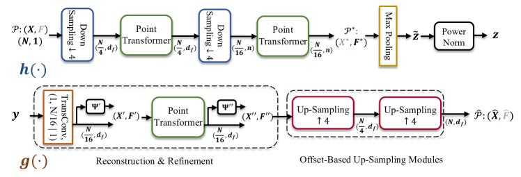
Figure 1: The detailed architecture of SEPT with an encoder $h(\cdot)$ and a decoder $g(\cdot)$. For clarity, we label the dimension information of the point cloud after each processing module. Take $(\frac{N}{4},d_{f})$ after the first point transformer at the encoder for an example, $\frac{N}{4}$ is the number of points after the point transformer and $d_{f}$ is the dimension of feature vectors.

Overcoming the above challenges requires the development of more efficient feature extraction modules and communication protocols. In this paper, we leverage the recent advances in deep joint source-channel coding (DeepJSCC) [7] and develop a deep learning-based encoding and decoding framework for wireless point cloud transmission. Our main contributions can be summarized as follows:

1. We present SEPT (SEmantic Point cloud Transmission), a tailored framework for efficient delivery of 3D point cloud over additive white Gaussian noise (AWGN) channels. To the best of our knowledge, this is the first work to utilize the autoencoder approach in designing communication systems specifically for point cloud transmission.

2. To efficiently extract semantic features and avoid the cliff and leveling effects, we develop novel DeepJSCC encoder and decoder architectures for 3D point cloud: At the transmitter, SEPT encodes the point cloud directly into a latent vector without voxelization. A flexible power normalization that judiciously assigns power to different point clouds is applied. At the receiver, as opposed to feeding the noisy latent vector directly into the up-sampling layer, we introduce a refinement layer that uses the Point Transformer[5] as the backbone to first denoise the latent vector. Finally, offset-based up-sampling layers are employed for point cloud reconstruction.

3. Extensive simulations are conducted to verify the reconstruction performance of SEPT. Comparisons with the octree-based digital scheme demonstrate significant performance gains achieved by SEPT. When compared with a more advanced benchmark that combines state-of-the-art deep learning-based compression [9] with Polar code, SEPT shows comparable reconstruction performance while simultaneously eliminating the cliff and leveling effects.

Related work: There have been many efforts in processing and understanding 3D point clouds using deep learning. The authors in [4] proposed PointNet that uses permutation-invariant operations, such as pointwise multilayer perceptrons (MLPs) and max-pooling, to extract features for point cloud classification and segmentation. The follow-up works improved the performance by using more advanced operations such as 3D convolution [10] and self-attention [5, 11, 12]. The most related line of work to ours is point cloud compression, for which different deep learning-based techniques have been proposed recently [2, 13, 14, 9]. Among them, [2] used deep neural networks to predict the occupancy probability for a certain node in the octree, exploiting the information from its parent node and sibling nodes. Then, an entropy model is used to generate the bit stream. Ref. [14] used multiple KPconv [10] and downsampling layers to progressively reduce the number of points and extract information from the points of previous layers, and an offset-based up-sampling algorithm was proposed to reconstruct the point clouds at the decoder. The authors in [9] used the point cloud transformer [11] as the backbone to enhance the compression performance.

There is also growing interest in utilizing DeepJSCC to develop semantic communication systems [7, 15]. It is shown in [7] that by end-to-end optimizing the DeepJSCC system, both the cliff and leveling effects can be eliminated. With such merits, researchers have actively applied DeepJSCC to different wireless channels, e.g., multi-path fading [16], MIMO [17], and relay channels [18], as well as different data sources, e.g., text [19], image [7, 20], speech [21, 22], video [23, 24], or even wireless channel state information [25].

For different channels and data sources, it is crucial to employ appropriate methods to harness their characteristics to maximize the potential of DeepJSCC. While convolutional neural network (CNN) based autoencoders have been successfully applied to many of these sources in the aforementioned works, three-dimensional point clouds constitute a much more challenging data source as they are unstructured and can be represented in an arbitrary coordinate system. Moreover, the points can be presented in any arbitrary order, which makes it difficult to apply any specified filter to capture the structure among neighbouring points. The main objective of semantic-oriented joint source-channel coding approach to wireless signal delivery is to extract the relevant features of the signal for the specified task, and to map similar features to similar channel inputs so that the reconstruction is robust against channel noise. However, the lack of structure in point clouds makes it highly challenging to apply CNN-based DeepJSCC techniques, despite their recent success in the wireless transmission of image and video sources.

II System Model

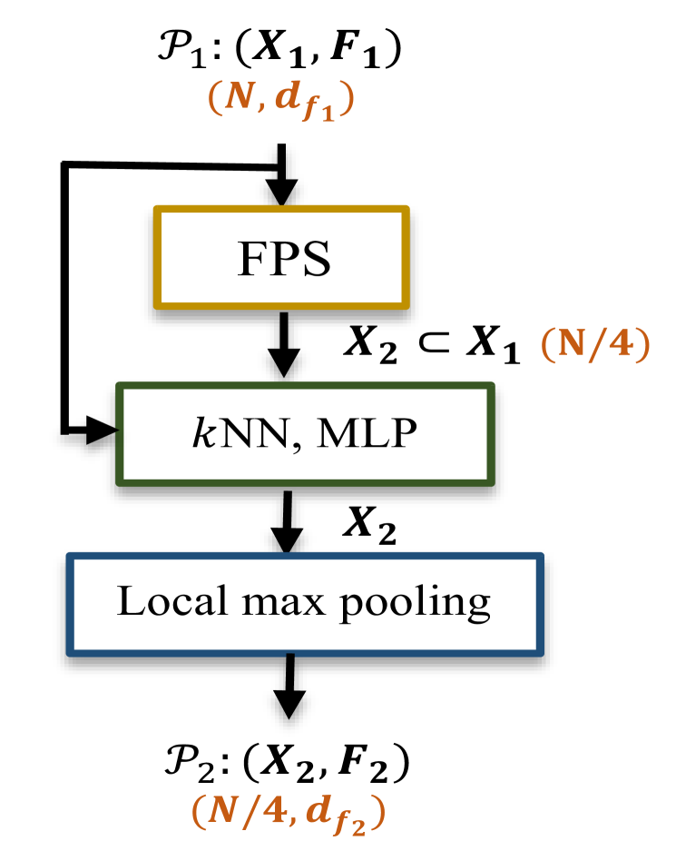
(a)

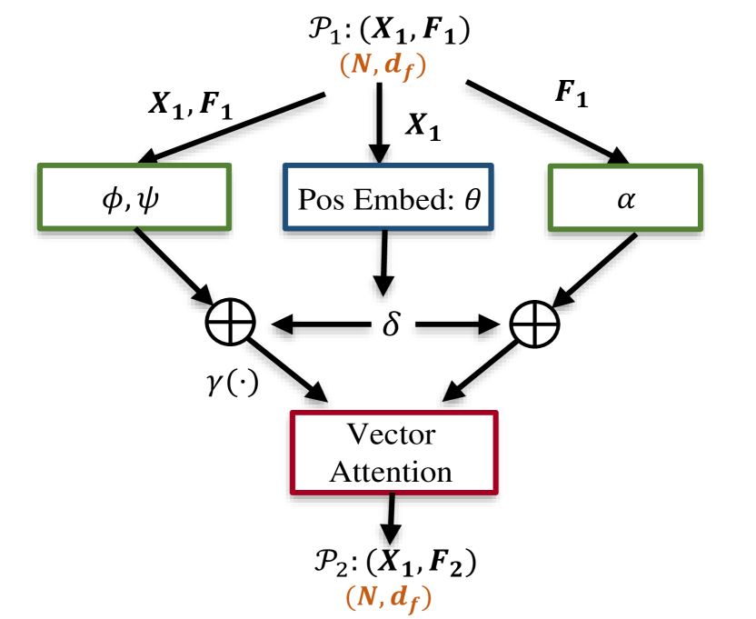
(b)

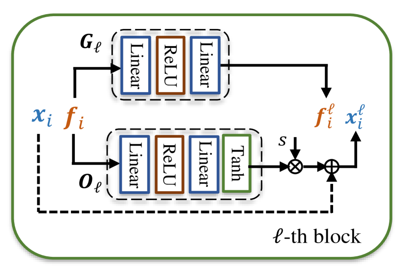
(c)

Figure 2: The inner architectures of (a) the downsampling module, (b) the point transformer layer, and (c) the $\ell$-th block of the offset-based up-sampling module, $\ell\in[1,L]$.

We consider transmitting a 3D point cloud over an AWGN channel. A point cloud can be expressed as $\mathcal{P}=(\bm{X},\bm{F})$, where $\bm{X}\triangleq\{\bm{x}_{i}\in\mathbb{R}^{3}\}$, $i\in[N]$, is a set of $N$ points in space, and $\bm{F}\triangleq\{\bm{f}_{i}\in\mathbb{R}^{d}\},i\in[N]$, is a set of features associated with each point in $\bm{X}$. In particular, this paper considers point clouds with no input attributes and focuses on transmitting only the coordinates $\bm{X}$. Following the convention, we set the input attributes $\bm{F}$ to an all-ones vector with $d=1$.

The detailed architecture of SEPT is presented in Fig. 1, where we denote the DeepJSCC encoder and decoder by $h(\cdot)$ and $g(\cdot)$, respectively. In the big picture, the encoder $h(\cdot)$ first maps the input 3D point cloud $\mathcal{P}$ to a latent vector $\bm{\tilde{z}}\in\mathbb{R}^{n}$ where $n$ is the available channel bandwidth. Then, we power normalize the latent vector to obtain a codeword $\bm{{z}}\in\mathbb{R}^{n}$ and transmit it to the receiver via discrete-time analog transmission (DTAT) [26]. In particular, instead of imposing a stringent power constraint such that the power of each codeword $\bm{z}$ is bounded by a power budget $nP/2$, we adopt a more flexible average power constraint [27]: $\mathbb{E}||\bm{z}||^{2}_{2}\leq nP/2,$ whereby the power of codewords associated with different point clouds can be adjusted judiciously. To achieve this, we record the moving mean $\mu$ and deviation $\sigma$ of $\bm{\tilde{z}}$ during the training phase. Then, in the inference phase, the latent vector $\tilde{\bm{z}}$ is normalized using $(\mu,\sigma)$, yielding

$$\bm{z}=(\bm{\tilde{z}}-\mu)/\sigma.$$ (1)

It is worth noting that the codeword $\bm{z}$ is converted to a complex vector, $\bm{z}^{\prime}\in\mathbb{C}^{n/2}$, when passing through the complex AWGN channel. The channel use per point (CPP) is given by $\frac{n}{2N}$.

At the receiver, the received signal $\bm{{y}}^{\prime}\in\mathbb{C}^{n/2}$ is a noisy version of $\bm{{z}}^{\prime}$:

$$\bm{{y}}^{\prime}=\bm{{z}}^{\prime}+\bm{w},$$ (2)

where $\bm{w}\in\mathbb{C}^{n/2}$ denotes a complex AWGN vector with independent and identically distributed elements, $\bm{w}\sim\mathcal{CN}(0,N_{0})$. The channel signal-to-noise ratio (SNR) is defined as $\mathrm{SNR}=10\log_{10}{\frac{P}{N_{0}}}$. Without loss of generally, we assume $P=1$ in the sequel. Upon receiving $\bm{{y}}^{\prime}$, we first convert it to a real vector $\bm{y}\in\mathbb{R}^{n}$ and feed it into the decoder $g(\cdot)$ to obtain a reconstructed point cloud $\hat{\mathcal{P}}$.

III Methodology

This section details our design of the encoder and decoder functions using neural network architectures, and explains how features are extracted from the original point cloud $\mathcal{P}$ via downsampling and self-attention layers and how the point cloud $\hat{\mathcal{P}}$ is reconstructed from the noisy latent vector via refinement and up-sampling layers.

III-A SEPT encoder

The encoder of SEPT consists of three main modules: downsampling, self-attention, and max pooling, as shown in Fig. 1.

Downsampling. The objective of the downsampling module is to reduce the number of points in the input point cloud. Let $\mathcal{P}_{1}=(\bm{X}_{1},\bm{F}_{1})$ and $\mathcal{P}_{2}=(\bm{X}_{2},\bm{F}_{2})$ denote the input and output point clouds of a downsampling module, respectively, where $\bm{X}_{2}\subset\bm{X}_{1}$. In particular,

• In order to achieve a more representative point cloud, it is crucial to disperse the selected points, i.e., $\bm{X}_{2}$, as widely as possible, ensuring sufficient coverage across $\bm{X}_{1}$.

• The clipped points of $\mathcal{P}_{1}$ will be embedded into the features of $\mathcal{P}_{2}$ to facilitate reconstruction at the receiver.

To the above ends, SEPT uses the farthest point sampling (FPS) algorithm to generate $\bm{X}_{2}$, as shown in Fig. 2(a). To generate the feature vector of the $i$-th point in $\bm{X}_{2}$, denoted by $\bm{f}^{(2)}_{i}\in\mathbb{R}^{d_{f_{2}}}$, we first find its $k$-nearest neighbors within a given radius $r$ in $\bm{X}_{1}$ and denote them by $\mathbb{N}(i)$. Then, we concatenate the feature vectors with their coordinates of the points in $\mathbb{N}(i)$ and organise them into a tensor, denoted by $\bm{T}_{\mathbb{N}(i)}\in\mathbb{R}^{(d_{f_{1}}+3)}\times k\times N_{1}$ where $N_{1}$ denotes the cardinality of $\bm{X}_{1}$, and feed this tensor to a 2D convolutional layer followed by batch normalization, ReLU, and max pooling. In each downsampling module, we set the cardinality of $\bm{X}_{2}$ to be $1/4$ of that of $\bm{X}_{1}$, i.e., $|\bm{X}_{2}|=|\bm{X}_{1}|/4$.

Self-Attention. In SEPT, each downsampling module is followed by a self-attention module [5], a point cloud processing technique that is capable of extracting rich neighboring information. Denote the input and output point clouds of the self-attention layer by $\mathcal{P}_{1}=(\bm{X}_{1},\bm{F}_{1})$ and $\mathcal{P}_{2}=(\bm{X}_{1},\bm{F}_{2})$, respectively. As shown in Fig. 2(b), the self-attention layer refines the features of each point in $\mathcal{P}_{1}$. The inner operations can be written as

$$\bm{f}^{(2)}_{i}\!=\!\!\sum_{j\in\mathbb{N}(i)}\!\text{Softmax}\big{(}\gamma(\phi(\bm{f}^{(1)}_{i})-\phi(\bm{f}^{(1)}_{j}))+\delta\big{)}\odot(\alpha(\bm{f}^{(1)}_{j})+\delta),$$

where $\bm{f}^{(2)}_{i}$ denotes the refined feature vector of the $i$-th point; $\gamma,\phi,\alpha:\mathbb{R}^{d_{f}}\rightarrow\mathbb{R}^{d_{f}}$ are realized by MLPs; $\delta=\theta(\bm{x}_{i}-\bm{x}_{j})$ is the positional information and $\theta:\mathbb{R}^{3}\rightarrow\mathbb{R}^{d_{f}}$ is an MLP layer for positional embedding; $\odot$ denotes the element-wise product. That is, we adopt vector attention [5], as opposed to the standard scalar dot-product attention used in language and vision transformer models, for better performance.

As shown in Fig. 1, after two consecutive downsampling and self-attention module pairs, the final downsized point cloud is obtained, which we denote by $\mathcal{P}^{*}=(\bm{X}^{*},\bm{F}^{*})$, where $\bm{X}^{*}\in\mathbb{R}^{(N/16)\times 3}$ and $\bm{F}^{*}\in\mathbb{R}^{(N/16)\times n}$. We emphasize that the features $\bm{F}^{*}$ are generated by neural networks and can be optimized to be robust to noise, thanks to end-to-end learning. On the other hand, the coordinates $\bm{X}^{*}$ are obtained from FPS and are susceptible to noise. Our empirical results indicate that $\bm{X}^{*}$ has to be transmitted to the receiver reliably via digital communications. Failure to do so results in a substantial degradation in the reconstruction performance of the point cloud. Digital transmission of $\bm{X}^{*}$, however, results in two problems: 1) the cliff and leveling effects; 2) excessive channel usage (detailed later in Section IV-B). In this context, SEPT eliminates the need for coordinate ($\bm{X}^{*}$) transmission and instead focuses solely on transmitting the features ($\bm{F}^{*}$) to the receiver. To be precise, SEPT learns to encode the global features in $\bm{F}^{*}$ and the decoder is trained to reconstruct the entire point cloud from the global features without the aid of the coordinates. By doing so, SEPT significantly reduces the amount of data that needs to be transmitted, leading to more efficient and streamlined communication.

Max Pooling. The last step at the encoder is to transform $\bm{F}^{*}\in\mathbb{R}^{(N/16)\times n}$ to the latent vector $\tilde{\bm{z}}\in\mathbb{R}^{n}$. A natural solution is to use an MLP for each $\bm{f}_{i}^{*}\in\mathbb{R}^{n}$. In contrast, SEPT applies max pooling over the $N/16$ points to generate the $n$-dimensional vector $\tilde{\bm{z}}$ where $n$ is the available channel bandwidth. The advantage of max pooling will be demonstrated in Section IV-B via an ablation study.

III-B SEPT decoder

The decoder of SEPT consists of two modules: latent reconstruction and refinement, and offset-based up-sampling.

Latent Reconstruction and Refinement. The latent reconstruction module takes the noisy latent vector as input to reconstruct $\mathcal{P}^{*}$. As shown in Fig. 1, given the received signal $\bm{y}$, we first use a TransConv layer, which is essentially a 1D deconvolution with a unit stride, to generate the initial estimate of $\bm{F}^{*}$, denoted by ${\bm{F}}^{\prime}\in\mathbb{R}^{(N/16)\times n}$. Then, we employ a coordinate reconstruction layer $\Psi^{\prime}:\mathbb{R}^{n}\rightarrow\mathbb{R}^{3}$, which is composed of MLP layers and a ReLU function, operates on each row of ${\bm{F}}^{\prime}$ to generate an initial estimate of the coordinates:

$${\bm{X}}^{\prime}=\Psi^{\prime}({\bm{F}}^{\prime}),$$ (3)

where ${\bm{X}}^{\prime}\in\mathbb{R}^{N/16\times 3}$. The initial estimates $({\bm{X}}^{\prime},{\bm{F}}^{\prime})$ can be erroneous due to noise. Therefore, we further use a self-attention module, denoted as SA, to refine the features:

$${\bm{F}}^{\prime\prime}=\text{SA}({\bm{X}}^{\prime},{\bm{F}}^{\prime}).$$ (4)

Next, a new coordinate reconstruction layer, $\Psi^{\prime\prime}$, is applied to ${\bm{F}}^{\prime\prime}$ to produce a refined estimation of coordinates, ${\bm{X}}^{\prime\prime}$. Our refinement module is shown to be very effective in denoising the coordinates and features. An ablation study will be provided in Section IV-B.

Offset-Based Up-Sampling. Finally, we employ an offset-based up-sampling module [14] on $({\bm{X}}^{\prime\prime},{\bm{F}}^{\prime\prime})$ for point cloud reconstruction. For the $i$-th point in the input point cloud, whose coordinates and features are denoted by $(\bm{x}_{i},\bm{f}_{i})$, this module generates $L$ new points $\{(\bm{x}_{i}^{\ell},\bm{f}_{i}^{\ell}),\ell\in[1,L]\}$ as:

$$\bm{x}_{i}^{\ell} =\bm{x}_{i}+s\cdot O_{\ell}(\bm{f}_{i}),$$ (5)

$$\bm{f}_{i}^{l} =G_{\ell}(\bm{f}_{i}),$$ (6)

where $O_{\ell}:\mathbb{R}^{d_{f}}\rightarrow[-1,1]^{3}$ is an MLP layer followed by a $\mathrm{tanh}$ function that aims to generate an offset vector; $G_{\ell}$ is comprised of MLPs and a ReLU function that maps the input feature to a new one with the same dimension. In particular, $s$ is a scaling factor for the offsets. Compared with [14], SEPT uses a relatively large $s=0.1$ to give the up-sampling module more freedom for better performance, considering the additional noise introduced by the wireless channel. The detailed architectures for $O_{\ell}$ and $G_{\ell}$ are shown in Fig. 2(c).

In SEPT, we use two up-sampling modules, and $L$ is set to $4$ in each module. Denoting by $\hat{\mathcal{P}}=(\hat{\bm{X}},\hat{\bm{F}})$ the final output of the up-sampling modules, the Chamfer distance between ${\bm{X}}$ and $\hat{\bm{X}}$, denoted by $d^{2}_{cd}({\bm{X}},\hat{\bm{X}})$, is used as the loss function:

$$\mathcal{L}_{\text{CD}}=\frac{1}{N}\sum_{\bm{x}\in\mathcal{P}}\min_{\bm{y}\in\hat{\mathcal{P}}}||\bm{x}-\bm{y}||^{2}_{2}+\frac{1}{N}\sum_{\bm{y}\in\hat{\mathcal{P}}}\min_{\bm{x}\in{\mathcal{P}}}||\bm{y}-\bm{x}||^{2}_{2}.$$ (7)

IV Numerical Experiments

This section presents the results of our numerical experiments to evaluate the reconstruction performance of SEPT. We consider the point cloud data from ShapeNet [28], which contains about $51000$ different shapes, and we sample each point cloud to $N=2048$ points using the FPS algorithm. In both the SEPT encoder and decoder, the dimension of the intermediate attributes is set to $d_{f}=256$ and the number of neurons in the MLPs of the coordinate reconstruction layer is set to $128$. During training, we adopt the Adam optimizer with a varying learning rate, which is initialized to 0.001 and reduced by a factor of $0.5$ every $20$ epochs. We set the number of epochs to $200$ and the batch size to $32$. Two conventional peak signal-to-noise ratio (PSNR) measures [29], D1 and D2, are adopted to evaluate the reconstruction quality. Specifically, $\text{D1}(\mathcal{A},\mathcal{B})$ measures the average point-to-point geometric distance between each point in point cloud $\mathcal{A}$ and its nearest neighbor in point cloud $\mathcal{B}$. To be precise, we first calculate the mean squared error, $e_{\mathcal{A},\mathcal{B}}^{D1}$:

$$e_{\mathcal{A},\mathcal{B}}^{D1} =\frac{1}{N}\sum_{\bm{a}_{i}\in\mathcal{A}}||\bm{a}_{i}-\bm{b}_{k}||_{2}^{2}$$

$$k =\operatorname*{arg\,min}_{j\in[N]}{||\bm{a}_{i}-\bm{b}_{j}||_{2}^{2}}.$$ (8)

then, D1 is calculated as [29]:

$$\text{D1}(\mathcal{A},\mathcal{B})=10\frac{3\gamma^{2}}{\max(e_{\mathcal{A},\mathcal{B}}^{D1},e_{\mathcal{B},\mathcal{A}}^{D1})},$$ (9)

where factor $3$ in the numerator is due to the 3D coordinates used in the representation, and the peak, $\gamma$, is set to unity due to the fact that the input points are normalized within the range $[0,1]$. Similarly, D2 evaluates the point-to-plane distance between $\mathcal{A}$ and $\mathcal{B}$ and the error term for D2 is defined as:

$$e_{\mathcal{A},\mathcal{B}}^{D2}=\frac{1}{N}\sum_{\bm{a}_{i}\in\mathcal{A}}(\bm{a}_{i}-\bm{b}_{k})\cdot\bm{n}_{i},$$ (10)

where $\bm{n}_{i}$ is the normal vector corresponding to $\bm{a}_{i}$ and $\bm{b}_{k}$ is the nearest neighbor of $\bm{a}_{i}$. After obtaining (10), we follow the same formula in (9) to calculate $\text{D2}(\mathcal{A},\mathcal{B})$.

Table I: D1 performance (in dB) comparison between max pooling and linear projection to generate the channel inputs ($n=300$).

$\mathrm{SNR}$	0 dB	5 dB	10 dB
Max Pooling	34.33	35.27	35.63
Linear Projection	26.41	30.22	31.27

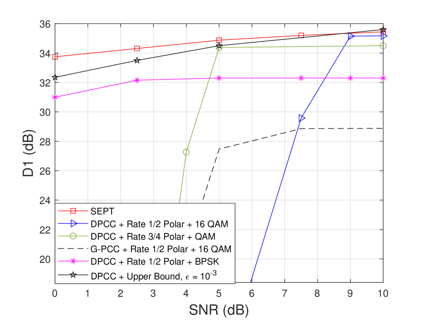
(a)

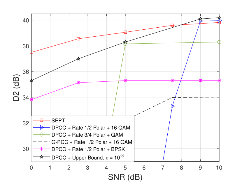
(b)

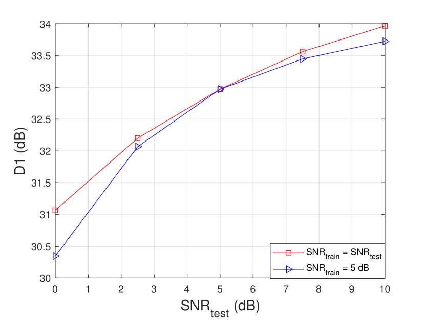
(c)

Figure 3: Reconstruction performances of SEPT: (a) $\&$ (b) the D1 and D2 performances, where $n=200$; (c) D1 versus the test SNR, where $n=50$ and the SEPT model is trained with $\mathrm{SNR}_{\text{train}}=5$ dB.

IV-A The reconstruction performance

We first evaluate the reconstruction performance of SEPT with various CPP and channel SNR values. Two separate source-channel coding schemes are considered as benchmarks. For source coding, the first benchmark uses the standard octree-based point cloud compression scheme: MPEG G-PCC [3]. The second benchmark uses the state-of-the-art deep learning-based point cloud compression scheme, which we name it as DPCC [9]. Both schemes are protected by Polar codes with rate $\{1/2,3/4\}$ and modulated by BPSK, QPSK, or 16QAM for transmission. We also provide the results for the DPCC delivered at finite block length converse bound [30] for a block error rate of $\epsilon=10^{-3}$.

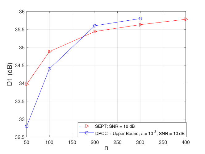
Figure 4: The reconstruction performance (D1) of the proposed SEPT with respect to different number of channel uses $n$. We fix the $\text{SNR}=10$ dB.

The simulation results are presented in Fig. 3 (a) and (b), where we fix the channel bandwidth to $n=200$. In the simulations, a specific SEPT model is trained for each channel SNR value. As shown, SEPT is significantly better than the separation based scheme with MPEG G-PCC, demonstrating its efficacy in feature extraction and robustness to channel noise. SEPT also outperforms the separation-based scheme with DPCC [9], especially in the low-SNR regime. Note that DPCC can achieve comparable performance to SEPT at certain SNRs, if proper coded modulation schemes are selected.

Next, we show how SEPT eliminates the cliff and leveling effects. To this end, Fig. 3(c) evaluates the performance of the SEPT model trained with a $\mathrm{SNR}_{\text{train}}=5$ dB under various channel conditions, $\mathrm{SNR}_{\text{test}}=\{0,2.5,5,7.5,10\}$ dB. For these simulations, we set $n=50$. As shown, the single SEPT model trained with $\mathrm{SNR}_{\text{train}}=5$ dB is robust to channel variations and performs well under various test SNRs. Importantly, SEPT eliminates the cliff and leveling effects, its performance degrades gracefully with the decrease in the test SNR and improves when the test SNR increases, while the digital benchmarks suffer from both the cliff and leveling effects if the modulation order remains unchanged, as shown in Fig. 3(a) and (b).

The performance of the proposed SEPT with respect to different number of channel uses $n$ are shown in Fig. 4. Two SNR values, $\{0,10\}$ dB, are considered and we compare the SEPT with the DPCC baseline delivered at finite length capacity. We can observe that D1 and D2 almost saturate when $n\geq 200$. This might be due to the max pooling operation at the transmitter focuses more on the global features while the fine details may be lost.

We also provide a visualization of the reconstructed point clouds with $n=300$ and $\mathrm{SNR}\in\{0,5\}$ dB. As shown in Fig. 5, SEPT yields visually pleasing results even when the $\mathrm{SNR}$ is as low as 0 dB.

IV-B Ablation study

This section performs ablation studies to evaluate different modules of SEPT.

Max pooling versus linear projection. As mentioned in Section III-A, to generate $\tilde{\bm{z}}$ from the feature vectors $\bm{F}^{*}\in\mathcal{R}^{N/16\times n}$, we can either use max pooling to produce an $n$-dimensional vector or perform MLP layers on $\bm{F}^{*}$ to generate an $N/16\times t$ matrix satisfying $Nt/16\approx n$. For comparison, we set $n=300,t=3$ for the two schemes, and report the reconstruction performance with $\mathrm{SNR}=\{0,5,10\}$ dB in terms of D1 and D2 in Table I. It is confirmed that max pooling is superior to a linear projection.

The refinement networks at the decoder. The initial estimates of both the coordinates and the features, $\{\bm{{X}}^{\prime},\bm{{F}}^{\prime}\}$, obtained from the 1D deconvolution layer are noisy, and SEPT uses an additional self-attention layer and a coordinate estimation layer to refine these coordinates and features. In this simulation, we show the effectiveness of the proposed refinement neural network by comparing the Chamfer distance (7) between $\{{\mathcal{P}}^{\prime\prime},{\mathcal{P}}\}$ with that of $\{{\mathcal{P}}^{\prime},{\mathcal{P}}\}$, where $\mathcal{P}$ is the original point cloud. Simulations are performed with $n=300$ and $\mathrm{SNR}=0$ dB, and we have $\mathcal{L}_{\text{CD}}({\bm{X}}^{\prime},{\bm{X}})=0.76$ and $\mathcal{L}_{\text{CD}}({\bm{X}}^{\prime\prime},{\bm{X}})=0.018$ illustrating that the refinement layer provides a much more accurate reconstruction.

Transmitting downsampled coordinates. As stated in Section III-B, SEPT only transmits the features $\bm{F}^{*}$ of the downsized point cloud, but not the coordinates $\bm{X}^{*}$. For a comprehensive understanding of SEPT, we further explore a hybrid transmission scheme, where $\bm{X}^{*}$ is transmitted in the digital fashion while $\bm{F}^{*}$ is transmitted with DTAT. Note that this hybrid transmission strategy will still suffer from the cliff and leveling effects.

In this simulation, we consider a $\mathrm{SNR}=10$ dB and $n=200$. For the hybrid scheme, we first downsample the original point cloud to $\mathcal{P}^{*}$ with $64$ points and then perform max pooling to generate a latent vector $\tilde{\bm{z}}$ with $n=200$, as SEPT. Then, $\bm{X}^{*}$ is quantized, and the quantized bits are transmitted using $1/2$-rate Polar code, and 16QAM modulation. At $\mathrm{SNR}=10$ dB, this coded modulation scheme achieves zero error probability for coordinate transmission. At the receiver, the coordinate reconstruction layers are no longer needed, since accurate coordinates are already available. The features are refined and the up-sampling blocks are used to reconstruct the final point clouds with $N$ points. We observe a slight improvement in D1 by sending extra coordinate information from $35.4$ dB to $36.2$ dB. However, even if we consider a $16$-bit precision of the coordinates as in [14], the extra cost for transmitting the coordinates is $3072$ bits, occupying $\approx 900$ excessive complex channel uses (assuming capacity achieving codes), which is unacceptable, given that we only have $n=200$.

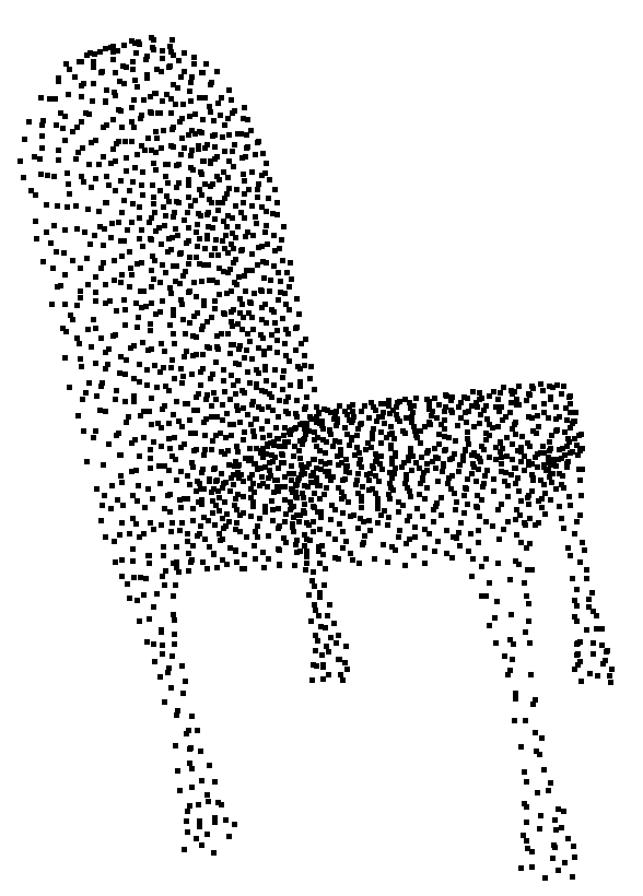
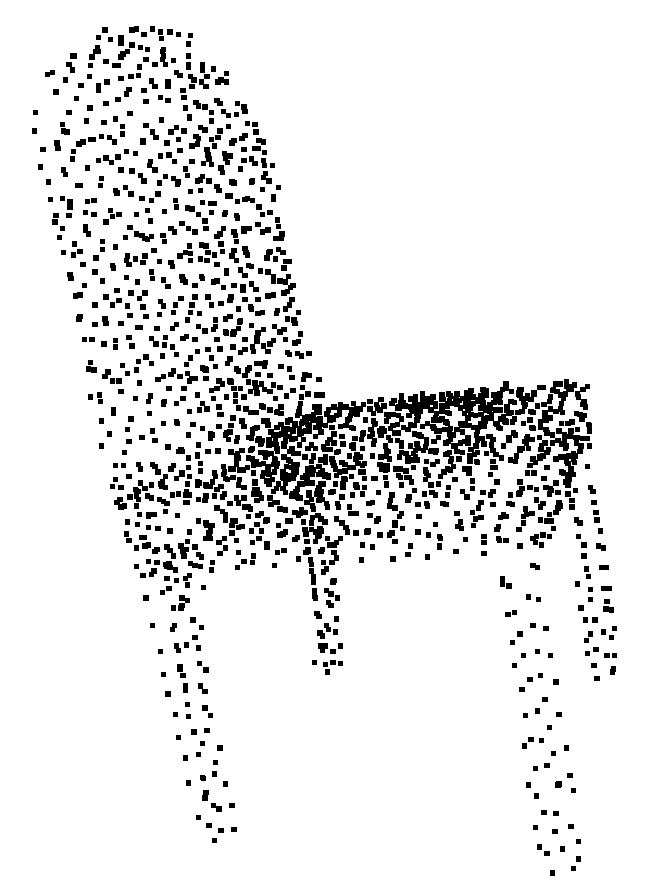
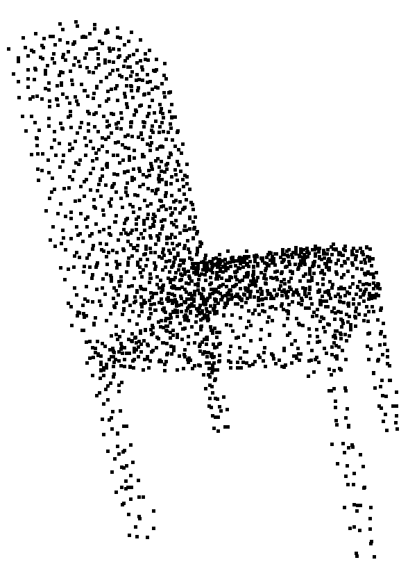
Figure 5: Visualization of reconstructed point clouds. Left: original $\mathcal{P}$; middle: $\hat{\mathcal{P}}$ with $n=300,\mathrm{SNR}=5$ dB; right: $\hat{\mathcal{P}}$ with $n=300,\mathrm{SNR}=0$ dB.

V Conclusion

Wireless transmission plays a pivotal role in enhancing the mobility and accessibility of 3D point clouds. With limited bandwidth, the SEPT framework proposed in this paper achieves efficient and robust wireless transmission of 3D point clouds, paving the way for realizing immersive user experiences in the metaverse, or collaborative sensing in vehicular networks. Our study highlights two key challenges that merit further investigation:

• The potential for a hybrid scheme that transmits both point cloud coordinates and features for improved performance, albeit at the expense of increased bandwidth utilization. A direction worthy of exploration involves designing a cost-effective hybrid scheme that strikes a balance between performance enhancement and bandwidth efficiency.

• Our findings indicate that the reconstruction performance reaches a saturation point as the CPP increases. This implies that certain intricate details of the point cloud are not fully preserved during feature extraction. To address this issue, it is crucial to develop new encoding and decoding architectures that effectively capture these fine details, enabling progressive performance improvements with higher CPP values.

References

- [1] R. B. Rusu and S. Cousins, “3D is here: Point Cloud Library,” in IEEE International Conference on Robotics and Automation, 2011.
- [2] L. Huang, S. Wang, K. Wong, J. Liu, and R. Urtasun, “OctSqueeze: Octree-structured entropy model for LiDAR compression,” in Proceedings of the IEEE/CVF Conference on Computer Vision and Pattern Recognition (CVPR), June 2020.
- [3] D. Graziosi, O. Nakagami, S. Kuma, A. Zaghetto, T. Suzuki, and A. Tabatabai, “An overview of ongoing point cloud compression standardization activities: Video-based (V-PCC) and geometry-based (G-PCC),” APSIPA Transactions on Signal and Information Processing, vol. 9, pp. 1–13, 2020.
- [4] C. R. Qi, H. Su, K. Mo, and L. J. Guibas, “Pointnet: Deep learning on point sets for 3D classification and segmentation,” in Proceedings of the IEEE conference on computer vision and pattern recognition, 2017, pp. 652–660.
- [5] H. Zhao, L. Jiang, J. Jia, P. H. Torr, and V. Koltun, “Point transformer,” in Proceedings of the IEEE/CVF international conference on computer vision, 2021, pp. 16 259–16 268.
- [6] P. de Oliveira Rente, C. Brites, J. Ascenso, and F. Pereira, “Graph-based static 3D point clouds geometry coding,” IEEE Transactions on Multimedia, vol. 21, no. 2, pp. 284–299, 2018.
- [7] E. Bourtsoulatze, D. B. Kurka, and D. Gündüz, “Deep joint source-channel coding for wireless image transmission,” IEEE Trans. Cognitive Commun. Netw., vol. 5, no. 3, pp. 567–579, 2019.
- [8] T. Fujihashi, T. Koike-Akino, T. Watanabe, and P. V. Orlik, “HoloCast+: Hybrid digital-analog transmission for graceful point cloud delivery with graph Fourier transform,” IEEE Transactions on Multimedia, vol. 24, pp. 2179–2191, 2021.
- [9] J. Zhang, G. Liu, D. Ding, and Z. Ma, “Transformer and upsampling-based point cloud compression,” in Proceedings of the 1st International Workshop on Advances in Point Cloud Compression, Processing and Analysis, 2022, pp. 33–39.
- [10] H. Thomas, C. R. Qi, J.-E. Deschaud, B. Marcotegui, F. Goulette, and L. J. Guibas, “Kpconv: Flexible and deformable convolution for point clouds,” in Proceedings of the IEEE/CVF international conference on computer vision, 2019, pp. 6411–6420.
- [11] M.-H. Guo, J.-X. Cai, Z.-N. Liu, T.-J. Mu, R. R. Martin, and S.-M. Hu, “Pct: Point cloud transformer,” Computational Visual Media, vol. 7, pp. 187–199, 2021.
- [12] C. Park, Y. Jeong, M. Cho, and J. Park, “Fast point transformer,” in Proceedings of the IEEE/CVF Conference on Computer Vision and Pattern Recognition, 2022, pp. 16 949–16 958.
- [13] J. Wang, D. Ding, Z. Li, and Z. Ma, “Multiscale point cloud geometry compression,” in 2021 Data Compression Conference (DCC). IEEE, 2021, pp. 73–82.
- [14] L. Wiesmann, A. Milioto, X. Chen, C. Stachniss, and J. Behley, “Deep compression for dense point cloud maps,” IEEE Robotics and Automation Letters, vol. 6, no. 2, pp. 2060–2067, 2021.
- [15] D. Gündüz, Z. Qin, I. E. Aguerri, H. S. Dhillon, Z. Yang, A. Yener, K. K. Wong, and C.-B. Chae, “Beyond transmitting bits: Context, semantics, and task-oriented communications,” IEEE J. Sel. Area Comm., 2022.
- [16] M. Yang, C. Bian, and H.-S. Kim, “OFDM-guided deep joint source channel coding for wireless multipath fading channels,” IEEE Transactions on Cognitive Communications and Networking, vol. 8, no. 2, pp. 584–599, 2022.
- [17] H. Wu, Y. Shao, C. Bian, K. Mikolajczyk, and D. Gündüz, “Vision transformer for adaptive image transmission over MIMO channels,” in IEEE International Conference on Communications (ICC), 2023.
- [18] C. Bian, Y. Shao, H. Wu, and D. Gunduz, “Deep joint source-channel coding over cooperative relay networks,” 2022.
- [19] N. Farsad, M. Rao, and A. Goldsmith, “Deep learning for joint source-channel coding of text,” in 2018 IEEE International Conference on Acoustics, Speech and Signal Processing (ICASSP), 2018, pp. 2326–2330.
- [20] J. Dai, S. Wang, K. Tan, Z. Si, X. Qin, K. Niu, and P. Zhang, “Nonlinear transform source-channel coding for semantic communications,” IEEE Journal on Selected Areas in Communications, vol. 40, no. 8, pp. 2300–2316, 2022.
- [21] Z. Weng, Z. Qin, X. Tao, C. Pan, G. Liu, and G. Y. Li, “Deep learning enabled semantic communications with speech recognition and synthesis,” IEEE Transactions on Wireless Communications, pp. 1–1, 2023.
- [22] T. Han, Q. Yang, Z. Shi, S. He, and Z. Zhang, “Semantic-preserved communication system for highly efficient speech transmission,” IEEE Journal on Selected Areas in Communications, vol. 41, no. 1, pp. 245–259, 2023.
- [23] T.-Y. Tung and D. Gündüz, “DeepWiVe: Deep-learning-aided wireless video transmission,” IEEE Journal on Selected Areas in Communications, vol. 40, no. 9, pp. 2570–2583, 2022.
- [24] S. Wang, J. Dai, Z. Liang, K. Niu, Z. Si, C. Dong, X. Qin, and P. Zhang, “Wireless deep video semantic transmission,” IEEE Journal on Selected Areas in Communications, vol. 41, no. 1, pp. 214–229, 2023.
- [25] M. B. Mashhadi, Q. Yang, and D. Gündüz, “Cnn-based analog csi feedback in fdd mimo-ofdm systems,” in IEEE International Conference on Acoustics, Speech and Signal Processing (ICASSP), 2020, pp. 8579–8583.
- [26] Y. Shao and D. Gunduz, “Semantic communications with discrete-time analog transmission: A PAPR perspective,” IEEE Wireless Communications Letters, vol. 12, no. 3, pp. 510–514, 2022.
- [27] E. Ozfatura, Y. Shao, A. G. Perotti, B. M. Popović, and D. Gündüz, “All you need is feedback: Communication with block attention feedback codes,” IEEE Journal on Selected Areas in Information Theory, vol. 3, no. 3, pp. 587–602, 2022.
- [28] A. X. Chang, T. Funkhouser, L. Guibas, P. Hanrahan, Q. Huang, Z. Li, S. Savarese, M. Savva, S. Song, H. Su et al., “Shapenet: An information-rich 3D model repository,” arXiv preprint arXiv:1512.03012, 2015.
- [29] “Common test conditions for point cloud compression,” ISO/IEC JTC1/SC29/WG11 MPEG output document N19084, Feb. 2020.
- [30] Y. Polyanskiy, H. V. Poor, and S. Verdu, “Channel coding rate in the finite blocklength regime,” IEEE Transactions on Information Theory, vol. 56, no. 5, pp. 2307–2359, 2010.