Ziv-Zakai-type error bounds for general statistical models

Abstract

I propose Ziv-Zakai-type lower bounds on the Bayesian error for estimating a parameter $\beta:\Theta\to\mathbb{R}$ when the parameter space $\Theta$ is general and $\beta(\theta)$ need not be a linear function of $\theta$.

I Introduction

The Ziv-Zakai family of lower bounds on the Bayesian error of parameter estimation are useful tools in estimation theory, as they are often reasonable to compute, do not require the involved functions to be differentiable, and may be much tighter than the Cramér-Rao-type bounds for certain problems Ziv and Zakai (1969); Bell et al. (1997); Van Trees and Bell (2007); Tsang (2012); Berry et al. (2015); Jeong et al. (2023). When the underlying parameter $\theta\in\Theta$ is vectoral in Euclidean parameter space $\Theta=\mathbb{R}^{p}$, Bell and coworkers have proposed some extended Ziv-Zakai bounds Bell et al. (1997), but they work only when the parameter of interest $\beta(\theta)$ is a linear function of $\theta$. Jeong, Dytso, and Cardone recently generalized Bell’s bounds for any prior probability measure on a Euclidean $\Theta$ and $\beta(\theta)=\theta$ Jeong et al. (2023). This paper generalizes the bounds for a general parameter space $\Theta$ and a general function $\beta:\Theta\to\mathbb{R}$ as the parameter of interest.

II Main result

Let $Y$ be the observation in a Borel space $(\mathcal{Y},\Sigma_{\mathcal{Y}})$ and $P_{\theta}$ be its probability measure conditioned on a hidden parameter $\theta\in\Theta$. In the Bayesian setting, the parameter is also a random variable in a Borel space $(\Theta,\Sigma_{\Theta})$; let $\pi$ be its prior probability measure. For clarity, I use $\theta$ only to denote a specific value in $\Theta$ and $X$ to denote the hidden parameter as a random variable in general. Let $\beta:\Theta\to\mathbb{R}$ be a parameter of interest and $\check{\beta}:\mathcal{Y}\to\mathbb{R}$ be an estimator. Define a distortion function $D:\mathbb{R}_{+}\to\mathbb{R}_{+}$ with $\mathbb{R}_{+}\equiv[0,\infty\rparen$ and the properties

$$D(x) \geq D(y)\quad\textrm{if }x\geq y,$$ (1)

$$D(0) =0,$$ (2)

$$D(x) \textrm{ is differentiable, with }\dot{D}(x)\equiv\derivative{D(x)}{x}.$$ (3)

The Bayesian error can then be defined as

$$\mathsf{E} \equiv\operatorname{\mathbb{E}}\quantity{D[|\check{\beta}(Y)-\beta(X)|]},$$ (4)

where $\operatorname{\mathbb{E}}$ denotes the expectation with respect to all random variables. For example, $\mathsf{E}$ is the mean-square error when $D(x)=x^{2}$.

Ziv-Zakai-type bounds are lower bounds on $\mathsf{E}$ in terms of the minimum error probability of a related binary-hypothesis-testing problem. Let the two hypotheses be

$$\mathcal{H}_{0}:Y \sim P_{\theta}, \mathcal{H}_{1}:Y \sim P_{\phi},$$ (5)

and let the prior probability of $\mathcal{H}_{0}$ be $q$. I denote the minimum error probability for this hypothesis-testing problem as $\Pi(\theta,\phi,q)$. I can now present the main result of this paper.

Theorem 1.

Let $t\in\mathbb{R}_{+}$. For each $t$, let $\Phi_{t},\Phi_{t}^{\prime}\in\Sigma_{\Theta}$ be two subsets of the parameter space, $\Sigma_{t}\equiv\{S\cap\Phi_{t}:S\in\Sigma_{\Theta}\}\equiv\Sigma_{\Theta}\cap\Phi_{t}$ and $\Sigma_{t}^{\prime}\equiv\Sigma_{\Theta}\cap\Phi_{t}^{\prime}$ be the restrictions (Tao, 2011, Sec. 1.4) of $\Sigma_{\Theta}$ to $\Phi_{t}$ and $\Phi_{t}^{\prime}$, respectively, and $T_{t}:\Phi_{t}\to\Phi_{t}^{\prime}$ be a $\Sigma_{t}/\Sigma_{t}^{\prime}$-measurable map such that there exists a measure $\pi_{t}$ on $(\Phi_{t},\Sigma_{t})$ satisfying

$$\pi =\pi_{t}T_{t}^{-1}\quad\textrm{on }(\Phi_{t}^{\prime},\Sigma_{t}^{\prime}),$$ (6)

and

$$\beta(T_{t}(\theta))\geq\beta(\theta)+t\quad\textrm{almost everywhere on $\Phi_{t}$ with respect to $\pi_{t}$.}$$ (7)

Moreover, assume that both $\pi$ and $\pi_{t}$ are dominated by a reference measure $\mu$ on $(\Phi_{t},\Sigma_{t})$ and their densities are denoted as

$$f \equiv\derivative{\pi}{\mu},$$ (8)

$$f_{t} \equiv\derivative{\pi_{t}}{\mu}.$$ (9)

Then

$$\mathsf{E} \geq\mathsf{Z}_{1}\equiv\frac{1}{2}\int_{0}^{\infty}dt\dot{D}\quantity(\frac{t}{2})\mathcal{V}g_{1}(t),$$ (10)

$$g_{1}(t) \equiv\int_{\Phi_{t}}d\mu(\theta)\quantity[f(\theta)+f_{t}(\theta)]\Pi\quantity(\theta,T_{t}(\theta),\frac{f(\theta)}{f(\theta)+f_{t}(\theta)}),$$ (11)

where

$$\mathcal{V}g(t) \equiv\sup_{t^{\prime}:t^{\prime}\geq t}g(t^{\prime})$$ (12)

is the valley-filling operator Van Trees and Bell (2007). A more convenient bound is

$$\mathsf{E} \geq\mathsf{Z}_{2}\equiv\frac{1}{2}\int_{0}^{\infty}dt\dot{D}\quantity(\frac{t}{2})\mathcal{V}g_{2}(t),$$ (13)

$$g_{2}(t) \equiv 2\int_{\Phi_{t}}d\mu(\theta)\min\quantity{f(\theta),f_{t}(\theta)}\Pi\quantity(\theta,T_{t}(\theta),0.5).$$ (14)

Proof.

With the given properties of $D$, the error can be expressed as

$$\mathsf{E} =\frac{1}{2}\int_{0}^{\infty}dt\dot{D}\quantity(\frac{t}{2})\Pr\quantity(|\check{\beta}-\beta|\geq\frac{t}{2}),$$ (15)

where $\Pr$ denotes the probability. Write

$$\Pr\quantity(|\check{\beta}-\beta|\geq\frac{t}{2}) =\Pr\quantity(\check{\beta}\geq\beta(X)+\frac{t}{2})+\Pr\quantity(\check{\beta}<\beta(X)-\frac{t}{2}).$$ (16)

The first probability on the right-hand side of Eq. (16) can be bounded as

$$\Pr\quantity(\check{\beta}\geq\beta(X)+\frac{t}{2}) \geq\int_{\Phi_{t}}d\mu(\theta)f(\theta)\Pr\quantity(\check{\beta}\geq\beta(\theta)+\frac{t}{2}|X=\theta),$$ (17)

while the second probability can be bounded as

$$\Pr\quantity(\check{\beta}<\beta(X)-\frac{t}{2}) \geq\int_{\theta\in\Phi_{t}^{\prime}}d\pi(\theta)\Pr\quantity(\check{\beta}<\beta(\theta)-\frac{t}{2}|X=\theta)$$ (18)

$$=\int_{\phi\in\Phi_{t}}d\pi_{t}(\phi)\Pr\quantity(\check{\beta}<\beta(T_{t}(\phi))-\frac{t}{2}|X=T_{t}(\phi))$$ (19)

$$\geq\int_{\phi\in\Phi_{t}}d\mu(\phi)f_{t}(\phi)\Pr\quantity(\check{\beta}<\beta(\phi)+\frac{t}{2}|X=T_{t}(\phi)),$$ (20)

where Eq. (19) comes from Eq. (6) and the change-of-variable formula (Billingsley, 1995, Theorem 16.13) and Eq. (20) comes from Eqs. (7) and (9). Equation (16) can then be bounded as

$$\Pr\quantity(|\check{\beta}-\beta|\geq\frac{t}{2}) \geq g(t)\equiv\int_{\Phi_{t}}d\mu(\theta)\left[f(\theta)\Pr\quantity(\check{\beta}\geq\beta(\theta)+\frac{t}{2}|X=\theta)\right.$$

$$\quad\left.+f_{t}(\theta)\Pr\quantity(\check{\beta}<\beta(\theta)+\frac{t}{2}|X=T_{t}(\theta))\right]$$ (21)

$$=\int_{\Phi_{t}}d\mu(\theta)[f(\theta)+f_{t}(\theta)]\left[\frac{f(\theta)}{f(\theta)+f_{t}(\theta)}\Pr\quantity(\check{\beta}\geq\beta(\theta)+\frac{t}{2}|X=\theta)\right.$$

$$\quad\left.+\frac{f_{t}(\theta)}{f(\theta)+f_{t}(\theta)}\Pr\quantity(\check{\beta}<\beta(\theta)+\frac{t}{2}|X=T_{t}(\theta))\right].$$ (22)

The expression in the square brackets can be regarded as the error probability of a decision rule for a related hypothesis-testing problem and lower-bounded by $\Pi(\theta,T_{t}(\theta),f/(f+f_{t}))$. A lower bound $g_{1}(t)$ given by Eq. (11) on $\Pr(|\check{\beta}-\beta|\geq t/2)$ then results. Since $\Pr(|\check{\beta}-\beta|\geq t/2)$ is a nonincreasing function of $t$,

$$\Pr(|\check{\beta}-\beta|\geq\frac{t}{2}) \geq\Pr(|\check{\beta}-\beta|\geq\frac{t^{\prime}}{2})\geq g_{1}(t^{\prime}),\quad\forall t^{\prime}\geq t,$$ (23)

the valley-filling operator $\mathcal{V}$ can be applied to $g_{1}$ to obtain a tighter bound, and Eq. (10) results.

Equations (13) and (14) can be obtained similarly by starting with Eq. (21), using the bound

$$g(t) \geq 2\int_{\Phi_{t}}d\mu(\theta)\min\quantity{f(\theta),f_{t}(\theta)}\left[\frac{1}{2}\Pr\quantity(\check{\beta}\geq\beta(\theta)+\frac{t}{2}|X=\theta)\right.$$

$$\quad\left.+\frac{1}{2}\Pr\quantity(\check{\beta}<\beta(\theta)+\frac{t}{2}|X=T_{t}(\theta))\right],$$ (24)

and lower-bounding the expression in the square brackets by $\Pi(\theta,T_{t}(\theta),0.5)$. ∎

Remark 1.

At each $t$, $T_{t}$ and its domain $\Phi_{t}$—where $T_{t}$ satisfies Eq. (7)—may be picked to maximize $g_{1}(t)$ or $g_{2}(t)$ and produce the tightest bounds. If a $T_{t}$ can be found such that Eq. (7) is an equality, then Eq. (20) is an equality as well, and the bounds may be improved. For a chosen $T_{t}$, its domain $\Phi_{t}$ should also be as big as Theorem 1 allows.

Remark 2.

Note that $\pi_{t}$ may not be a probability measure, as the pushforward measure $\pi_{t}T_{t}^{-1}$ is required to match the given prior $\pi$ only on a subset $\Phi_{t}^{\prime}$ of the parameter space.

Remark 3.

It is straightforward to generalize Theorem 1 for quantum problems via quantum lower bounds on $\Pi$ Tsang (2012); Berry et al. (2015).

III Examples

Example 1.

If $\Theta=\mathbb{R}^{p}$, $\beta=u^{\top}\theta$, and $T_{t}(\theta)=\theta+vt$ with $u^{\top}v=1$, where $\top$ denotes the matrix transpose, $\theta$, $u$, and $v$ are all real column vectors of dimension $p$, and $u$ and $v$ do not depend on $\theta$, then one can pick $\Phi_{t}=\Phi_{t}^{\prime}=\Theta$, $d\mu(\theta)=d^{p}\theta$, and $f_{t}(\theta)=f(\theta+vt)$, such that Theorem 1 becomes the extended Ziv-Zakai bounds in Ref. Bell et al. (1997).

Example 2.

Let $\Theta=\mathbb{R}^{p}$ and the parameter of interest be the Euclidean norm

$$\beta(\theta) =\|\theta\|\equiv\sqrt{\theta^{\top}\theta}.$$ (25)

Suppose that the observation conditioned on each $\theta\in\Theta$ follows the linear Gaussian model $Y\sim N(\theta,\sigma^{2}I)$, where $I$ is the identity matrix. Previous Ziv-Zakai bounds are inapplicable because $\beta(\theta)$ here is a nonlinear function of $\theta$.

It is well known that

$$\Pi(\theta,T_{t}(\theta),0.5) =Q\quantity(\frac{\|\theta-T_{t}(\theta)\|}{2\sigma}),$$ (26)

where $Q(x)\equiv\Pr(Z\geq x)$ for a standard normal $Z$. It is also straightforward to show that

$$T_{t}(\theta) =\theta+\frac{\theta}{\|\theta\|}t$$ (27)

minimizes $\|\theta-T_{t}(\theta)\|$ subject to the constraint $\beta(T_{t}(\theta))=\|T_{t}(\theta)\|\geq\beta(\theta)+t=\|\theta\|+t$, and the minimum $\|\theta-T_{t}(\theta)\|$ is equal to $t$. Equation (13) for the mean-square error becomes

$$\mathsf{Z}_{2} =\int_{0}^{\infty}dtt\mathcal{V}\quantity[A(t)Q\quantity(\frac{t}{2\sigma})],$$ (28)

$$A(t) \equiv\int_{\Phi_{t}}d\mu\min\quantity{f,f_{t}}.$$ (29)

In some asymptotic limit of high signal-to-noise ratio (SNR), $Q(t/2\sigma)$ is expected to be concentrated near $t=0$ and much sharper than $A(t)$, so $A(t)$ can be approximated as $A(t)\approx A(0)=1$, leading to

$$\mathsf{Z}_{2} \approx\int_{0}^{\infty}dttQ\quantity(\frac{t}{2\sigma})=\sigma^{2}.$$ (30)

For an example of $A(t)$, consider a uniform prior density with respect to $d\mu(\theta)=d^{p}\theta$ for $\|\theta\|\leq R$, expressed as

$$f(\theta) =\frac{1}{V_{p}R^{p}}[\|\theta\|\leq R],$$ (31)

where $V_{p}$ is the volume of the unit ball in $p$ dimensions and $[\cdot]$ denotes the Iverson bracket. To compute $f_{t}$, one can pick $\Phi_{t}=\Theta-\{0\}$ and $\Phi_{t}^{\prime}=\{\theta\in\Theta:\|\theta\|>t\}$ such that $T_{t}$ is bijective and

$$f_{t}(\theta) =f(T_{t}(\theta))|\det D(\theta)|,$$ (32)

where $D_{jk}(\theta)\equiv\partialderivative*{[T_{t}(\theta)]_{j}}{\theta_{k}}$ is the Jacobian matrix (Billingsley, 1995, Theorem 17.2). With some effort, it can be shown that

$$f_{t}(\theta) =\frac{1}{V_{p}R^{p}}[\|\theta\|\leq R-t]\quantity(1+\frac{t}{\|\theta\|})^{p-1},$$ (33)

$$\min\quantity{f,f_{t}} =\frac{1}{V_{p}R^{p}}[\|\theta\|\leq R-t],$$ (34)

$$A(t) =\quantity(1-\frac{t}{R})^{p}[t\leq R].$$ (35)

The width of $A(t)$ is roughly $R/p$, so the high-SNR regime can be reached if $\sigma\ll R/p$.

$\mathsf{Z}_{2}$ can be compared with a Bayesian Cramér-Rao bound in a high-SNR regime Gill and Levit (1995); Tsang (2020) given by

$$\mathsf{E} \geq\mathsf{C}\approx\operatorname{\mathbb{E}}\quantity(u^{\top}J^{-1}u)=\sigma^{2}, u_{j} \equiv\partialderivative{\beta}{\theta_{j}}=\frac{\theta_{j}}{\beta}, J^{-1}=\sigma^{2}I,$$ (36)

where $J$ is the Fisher information matrix.

While the two bounds $\mathsf{Z}_{2}$ and $\mathsf{C}$ in Example 2 look identical, note that Cramér-Rao-type bounds in general require $f(\theta)$, $P_{\theta}$, and $\beta(\theta)$ to be differentiable in some way, whereas Theorem 1 here does not. More dramatic differences between the two types of bounds may be obtained when the observation model is nonlinear or non-Gaussian.

Another problem with existing Bayesian Cramér-Rao bounds Van Trees and Bell (2007); Gill and Levit (1995); Jupp (2010); Tsang (2020) is that they assume the parameter space $\Theta$ to be a finite-dimensional differentiable manifold such that differential geometry can be used, and it is unclear how they may be generalized for an infinite-dimensional $\Theta$, where differential geometry becomes a daunting subject. Theorem 1, on the other hand, can deal with an infinite-dimensional $\Theta$, at least in principle.

IV Geometric picture

It may be helpful to visualize $T_{t}$ in terms of a game in the parameter space, as shown in Fig. 1. $\beta(\theta)$ sets the difficulty levels of the game as a function of the player position $\theta\in\Theta$. $\{\theta:\beta(\theta)=C\}$ for a constant $C$ then specifies a surface of constant difficulty, which I call a stage. Each player starts at a position $\phi\in\Phi_{t}$ and moves to a final position $T_{t}(\phi)$ while satisfying certain rules. $t$ is the transport time; assume that it is given. Equation (7) is a rule that each player must reach a stage with difficulty level $\beta(T_{t}(\phi))$ at least $\beta(\phi)+t$, which is proportionate to the time taken. Since the stage with the minimum target level $\{\theta:\beta(\theta)=\beta(\phi)+t\}$ may not exist (i.e., the set may be empty), the inequality in Eq. (7) allows the player to reach a stage that exists at a higher level.

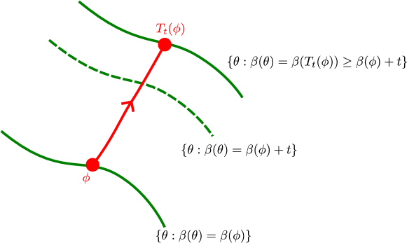
Figure 1: In the game picture, each player moves from the starting position $\phi$ to the final position $T_{t}(\phi)$ in the parameter space. $\beta(\theta)$ can be regarded as the difficulty level of a game as a function of player position $\theta\in\Theta$. $\beta(\theta)=C$ is then a surface of constant difficulty, or a stage. Each player is required to reach a stage with difficulty level at least $\beta(\phi)+t$.

To understand the role of $T_{t}$’s domain $\Phi_{t}$, suppose that each player is uniquely associated with one starting position $\phi$, which is used as their identification. If a player $\phi$ is unable to satisfy the rule at time $t$, then they should be removed from the game by excluding $\phi$ from $\Phi_{t}$. For example, if there is a supremum difficulty level $\beta_{\mathrm{sup}}\equiv\sup_{\theta\in\Theta}\beta(\theta)<\infty$, then a player $\phi$ with $\beta(\phi)+t>\beta_{\mathrm{sup}}$ can never satisfy Eq. (7) because there is no stage at the target level $\beta(T_{t}(\phi))\geq\beta(\phi)+t>\beta_{\mathrm{sup}}$ by time $t$. The player $\phi$ should hence be excluded from $\Phi_{t}$.

The measure $\pi_{t}$ assumed by Eq. (6) can be regarded as the initial distribution of the players on $\Phi_{t}$. After the movements specified by $T_{t}$, $\pi$ restricted to $\Phi_{t}^{\prime}$ is their final distribution. I call $(\Phi_{t},T_{t},\pi_{t})$ a flock. Since $\pi$ is given, the existence of $\pi_{t}$ given by Eq. (6) and its density $f_{t}$ given by Eq. (9) is another rule for the flock.

When there are many qualified flocks, one that produces a high $g_{1}(t)$ or $g_{2}(t)$ should be chosen. $g_{j}(t)$ can be regarded as a reward in the game and a definition of flock efficiency. For example, Ref. Bell et al. (1997) assumes that the stages $\beta(\theta)=u^{\top}\theta=C$ are parallel planes in the Euclidean space, and the flock are a family of parallel displacements $T_{t}(\theta)=\theta+vt$ with velocity $v$. If $u^{\top}v=1$, the flock for all starting positions in $\Phi_{t}=\Theta$ are just fast enough to reach their target stages. Subject to this constraint, $v$ is then chosen to produce a high $g_{j}(t)$. For another example, consider the choice of $T_{t}$ given by Eq. (27) in Example 2. It minimizes the distance $\|\theta-T_{t}(\theta)\|$, since the $\Pi(\theta,T_{t}(\theta),0.5)$ there is a decreasing function of the distance and the prior is ignored. The resulting flock move in radial directions, normal to the constant-$\beta$ surfaces, as one may heuristically expect from an efficient flock for the game.

It may be interesting to explore further this geometric picture in relation to the geometric picture of the Bayesian Cramér-Rao bounds Tsang (2020).

This research is supported by the National Research Foundation, Singapore, under its Quantum Engineering Programme (QEP-P7).

References

- Ziv and Zakai (1969) Jacob Ziv and Moshe Zakai, “Some lower bounds on signal parameter estimation,” IEEE Transactions on Information Theory 15, 386–391 (1969).
- Bell et al. (1997) Kristine L. Bell, Yossef Steinberg, Yariv Ephraim, and Harry L. Van Trees, “Extended ziv-zakai lower bound for vector parameter estimation,” IEEE Transactions on Information Theory 43, 624–637 (1997).
- Van Trees and Bell (2007) Harry L. Van Trees and Kristine L. Bell, eds., Bayesian Bounds for Parameter Estimation and Nonlinear Filtering/Tracking (Wiley-IEEE, Piscataway, 2007).
- Tsang (2012) Mankei Tsang, “Ziv-Zakai Error Bounds for Quantum Parameter Estimation,” Physical Review Letters 108, 230401 (2012).
- Berry et al. (2015) Dominic W. Berry, Mankei Tsang, Michael J. W. Hall, and Howard M. Wiseman, “Quantum Bell-Ziv-Zakai Bounds and Heisenberg Limits for Waveform Estimation,” Physical Review X 5, 031018 (2015).
- Jeong et al. (2023) Minoh Jeong, Alex Dytso, and Martina Cardone, “Functional properties of the ziv-zakai bound with arbitrary inputs,” ArXiv e-prints (2023), 10.48550/arXiv.2305.02970, 2305.02970 .
- Tao (2011) Terence Tao, An Introduction to Measure Theory (American Mathematical Society, Providence, 2011).
- Billingsley (1995) Patrick Billingsley, Probability and Measure, 3rd ed. (Wiley, New York, 1995).
- Gill and Levit (1995) Richard D. Gill and Boris Y. Levit, “Applications of the Van Trees inequality: A Bayesian Cramér-Rao bound,” Bernoulli 1, 59–79 (1995).
- Tsang (2020) Mankei Tsang, “Physics-inspired forms of the Bayesian Cramér-Rao bound,” Physical Review A 102, 062217 (2020).
- Jupp (2010) P. E. Jupp, “A van Trees inequality for estimators on manifolds,” Journal of Multivariate Analysis 101, 1814–1825 (2010).