A Unified Framework of Graph Information Bottleneck for Robustness and Membership Privacy

Abstract.

Graph Neural Networks (GNNs) have achieved great success in modeling graph-structured data. However, recent works show that GNNs are vulnerable to adversarial attacks which can fool the GNN model to make desired predictions of the attacker. In addition, training data of GNNs can be leaked under membership inference attacks. This largely hinders the adoption of GNNs in high-stake domains such as e-commerce, finance and bioinformatics. Though investigations have been made in conducting robust predictions and protecting membership privacy, they generally fail to simultaneously consider the robustness and membership privacy. Therefore, in this work, we study a novel problem of developing robust and membership privacy-preserving GNNs. Our analysis shows that Information Bottleneck (IB) can help filter out noisy information and regularize the predictions on labeled samples, which can benefit robustness and membership privacy. However, structural noises and lack of labels in node classification challenge the deployment of IB on graph-structured data. To mitigate these issues, we propose a novel graph information bottleneck framework that can alleviate structural noises with neighbor bottleneck. Pseudo labels are also incorporated in the optimization to minimize the gap between the predictions on the labeled set and unlabeled set for membership privacy. Extensive experiments on real-world datasets demonstrate that our method can give robust predictions and simultaneously preserve membership privacy.

1. Introduction

Graph Neural Networks (GNNs) have shown promising results in modeling graph-structured data such as social network analysis (Hamilton et al., 2017), finance (Wang et al., 2019), and drug discovery (Irwin et al., 2012). For graphs, both graph topology and node attributes are important for downstream tasks. Generally, GNNs adopt a message-passing mechanism to update a node’s representation by aggregating information from its neighbors. The learned node representation can preserve both node attributes and local structural information, which facilitates various tasks, especially semi-supervised node classification.

Despite their great success in modeling graphs, GNNs are at risk of adversarial attacks and privacy attacks. First, GNNs are vulnerable to adversarial attacks (Zügner and Günnemann, 2019; Zou et al., [n.d.]; Dai et al., 2018). An attacker can achieve various attack goals such as controlling predictions of target nodes (Dai et al., 2018) and degrading the overall performance (Zügner and Günnemann, 2019) by deliberately perturbing the graph structure and/or node attributes. For example, Nettack (Zügner et al., 2018) can mislead the target GNN to give wrong predictions on target nodes by poisoning the training graph with small perturbations on graph structure or node attributes. The vulnerability of GNNs largely hinders the adoption of GNNs in safety-critical domains such as finance and healthcare. Second, GNNs might leak private training data information under membership inference attacks (MIAs) (Shokri and Shmatikov, 2015; Olatunji et al., 2021). The membership inference attack can detect whether a target sample belongs to the training set. It can effectively distinguish the training samples even with black-box access to the prediction vectors of the target GNNs. This potential membership leakage threatens the privacy of the GNN models trained on sensitive data such as clinical records. For example, an attacker can infer the patient list from GNN-based chronic disease prediction on the patient network (Lu and Uddin, 2021).

Many efforts (Zhu et al., 2019; Entezari et al., 2020; Jin et al., 2020; Tang et al., 2020; Zhang and Zitnik, 2020; Dai et al., 2022b) have been taken to learn robust GNNs against adversarial attacks. For instance, robust aggregation mechanisms (Zhu et al., 2019; Chen et al., 2021; Geisler et al., 2021; Liu et al., 2021) have been investigated to reduce the negative effects of adversarial perturbations. A group of graph denoising methods (Zhang and Zitnik, 2020; Jin et al., 2020; Entezari et al., 2020; Dai et al., 2022a) is also proposed to remove/down-weight the adversarial edges injected by the attacker. Though they are effective in defending graph adversarial attacks, these methods may fail to preserve the membership privacy, which is also empirically verified in Sec. 5.3. For membership privacy-preserving, approaches such as adversarial regularization (Nasr et al., 2018) and differential privacy (Abadi et al., 2016; Papernot et al., 2016) are proposed for independent and identically distributed (i.i.d) data. However, in semi-supervised node classification, the size of labeled nodes is small and information on labeled nodes can be propagated to their neighbor nodes. These will challenge existing methods that generally process i.i.d data with sufficient labels. Work in membership privacy-preserving on GNNs is still limited (Olatunji et al., 2021), let alone robust and membership privacy-preserving GNNs. Therefore, in this paper, we focus on a novel problem of simultaneously defending adversarial attacks and membership privacy attacks with a unified framework.

One promising direction of simultaneously achieving robustness and membership privacy-preserving is to adopt the information bottleneck (IB) principle (Tishby et al., 2000) for node classification of GNNs. The IB principle aims to learn a code that maximally expresses the target task while containing minimal redundant information. In the objective function of IB, apart from the classification loss, a regularization is applied to constrain information irrelevant to the classification task in the bottleneck code. First, as IB encourages filtering out information irrelevant to the classification task, the noisy information from adversarial perturbations could be reduced, resulting in robust predictions (Alemi et al., 2016). Second, membership inference attack is feasible because of the difference between training and test samples in posteriors. As analyzed in Sec 3.5, the regularization in IB can constrain the mutual information between representations and labels on the training set, which can narrow the gap between training and test sets to avoid membership privacy leakage.

Though promising, there are still two challenges in applying IB principle for robust and membership privacy-preserving predictions on graphs. First, in graph-structured data, adversarial perturbations can happen in both node attributes and graph structures. However, IB for i.i.d data is only designed to extract compressed information from attributes. Simply extending the IB objective function used for i.i.d data to the GNN model may fail to filter out the structural noises. This problem is also empirically verified in Sec. 3.6. Second, in semi-supervised node classification, the size of labeled nodes is small. Without enough labels, the IB framework would have poor performance on test nodes. In this situation, the gap between labeled nodes and unlabeled test nodes can still be large even with the IB regularization term on labeled nodes, making it ineffective to defend MIA. Our empirical analysis in Sec. 3.5 also proves that this challenge is caused by lacking labels.

In an attempt to address these challenges, we propose a novel Robust and Membership Privacy-Preserving Graph Information Bottleneck (RM-GIB). RM-GIB develops a novel graph information bottleneck framework that adopts an attribute bottleneck and a neighbor bottleneck, which can handle the redundant information and adversarial perturbations in both node attributes and graph topology. Moreover, a novel self-supervisor is deployed to benefit the neighbor bottleneck in alleviating noisy neighbors to further improve the robustness. Since membership privacy-preserving with IB requires a large number of labels, RM-GIB collects pseudo labels on unlabeled nodes and combines them with provided labels in the optimization to guarantee membership privacy. In summary, our main contributions are:

• We investigate a new problem of developing a robust and membership privacy-preserving framework for graphs.

• We propose a novel RM-GIB that can alleviate both attribute and structural noises with bottleneck and preserve the membership privacy through incorporating pseudo labels in the optimization.

• Extensive experiments in various real-world datasets demonstrate the effectiveness of our proposed RM-GIB in defending membership inference and adversarial attacks.

2. Related Works

2.1. Graph Neural Networks

Graph Neural Networks (GNNs) (Kipf and Welling, 2016; Veličković et al., 2018; Ying et al., 2018; Bongini et al., 2021) have shown remarkable ability in modeling graph-structured data, which benefits various applications such as recommendation system (Ying et al., 2018), drug discovery (Bongini et al., 2021) and traffic analysis (Zhao et al., 2020). Generally, GNNs adopt a message-passing mechanism to iteratively aggregate the neighbor information to augment the representation learning of center nodes. For instance, in each layer of GCN (Kipf and Welling, 2016), the representations of neighbors and the center node will be averaged, followed by a non-linear transformation such as ReLU. GAT (Veličković et al., 2018) deploys an attention mechanism in the neighbor aggregation to benefit the representation learning. Recently, many extensions and improvements have been made to address various challenges in graph learning (Dai and Wang, 2021a; Qiu et al., 2020; Dai et al., 2021). For example, new frameworks of GNNs such LW-GCN (Dai et al., 2022c) are designed to handle the graph with heterophily. FairGNN (Dai and Wang, 2021a) is proposed to mitigate the bias of predictions of GNNs. Various self-supervised GNNs (Qiu et al., 2020; Dai and Wang, 2021b) have been explored to learn better representations. However, despite the great achievements, GNNs are vulnerable to adversarial (Zügner et al., 2018) and privacy attacks (Olatunji et al., 2021), which largely constrain the applications of GNNs in safety-critical domains such as bioinformatics and finance.

2.2. Robust Graph Learning

Extensive studies (Wu et al., 2019b; Zügner et al., 2018; Zügner and Günnemann, 2019; Dai et al., 2023) have shown that GNNs are vulnerable to adversarial attacks. Attackers can inject a small number of adversarial perturbations on graph structures and/or node attributes for their attack goals such as reducing overall performance (Zügner and Günnemann, 2019; Zou et al., [n.d.]) or controlling predictions of target nodes (Zügner et al., 2018; Dai et al., 2023).

Recently, many efforts have been taken to defend against adversarial attacks (Zhu et al., 2019; Entezari et al., 2020; Jin et al., 2020; Tang et al., 2020; Dai et al., 2022b), which can be roughly divided into three categories, i.e., adversarial training, robust aggregation, and graph denoising. In adversarial training (Xu et al., 2019), the GNN model is forced to give similar predictions for a clean sample and its adversarially perturbed version to achieve robustness. The robust aggregation methods (Zhu et al., 2019; Geisler et al., 2021; Liu et al., 2021) design a new message-passing mechanism to restrict the negative effects of adversarial perturbations. Some efforts in adopting Gaussian distributions as hidden representations (Zhu et al., 2019), aggregating the median value of each neighbor embedding dimension (Geisler et al., 2021), and incorporating $l_{1}$-based graph smoothing (Liu et al., 2021). In graph denoising methods (Jin et al., 2020; Wu et al., 2019b; Entezari et al., 2020; Dai et al., 2022a; Li et al., 2022), researchers propose various methods to identify and remove/down-weight the adversarial edges injected by the attacker. For example, Wu et al. (Wu et al., 2019b) propose to prune the perturbed edges based on the Jaccard similarity of node features. Pro-GNN (Jin et al., 2020) learns a clean graph structure by low-rank constraint. RS-GNN (Dai et al., 2022a) introduces a feature similarity weighted edge-reconstruction loss to train the link predictor which can down-weight the noisy edges and predict the missing links. However, these methods do not consider defense against membership inference attacks; On the contrary, the proposed RM-GIB can simultaneously defend against both adversarial attacks and membership inference attacks.

2.3. Membership Privacy Preservation

Membership inference attack (MIA) (Shokri and Shmatikov, 2015; Olatunji et al., 2021) is a type of privacy attack that aims to identify whether a sample belongs to the training set. The main idea of MIA is to learn a binary classifier on patterns such as posteriors that training and test samples exhibit different distributions. The membership leakage will largely threaten the privacy of the model trained on sensitive data such as medical records. Many studies (Shokri et al., 2017; Hayes et al., 2017; Choquette-Choo et al., 2021; Nasr et al., 2018; Abadi et al., 2016) have been conducted to defend against the membership inference attack on models trained on i.i.d data. The overfitting on the training samples leads to the difference between training samples and test samples in terms of posteriors and other patterns, which makes the membership inference attack feasible. Hence, a group of MIA defense methods propose to reduce the generalization gap through various regularization techniques. For example, L2 regularization (Shokri et al., 2017), weight normalization (Hayes et al., 2017), and dropout (Salem et al., 2018; Choquette-Choo et al., 2021) have been investigated for membership privacy preservation. Adversarial regularization (Nasr et al., 2018) is also explored to reduce the posterior distribution difference between training and test samples. Another type of defense (Abadi et al., 2016; Chaudhuri et al., 2011; Papernot et al., 2016) is to apply differentially private mechanisms such as DP-SGD (Abadi et al., 2016). These mechanisms generally add noise to gradients, model parameters, or outputs to achieve membership privacy guarantee. The above membership inference attack and defense methods are mainly on i.i.d data.

Recently, several seminal works (Olatunji et al., 2021; He et al., 2021; Wu et al., 2021) show that GNNs also suffer from MIA. However, defending MIA on graphs is rarely explored (Olatunji et al., 2021). Olatunji et al. (Olatunji et al., 2021) propose to inject noise to the posteriors or sample neighbors in the aggregation to protect the membership privacy on node classification. However, it will largely sacrifice the node classification performance to achieve membership privacy. On the contrary, our method combines the proposed novel graph IB and pseudo labels to give accurate and membership privacy-preserving predictions. Moreover, our framework is robust to both MIA and adversarial attacks.

2.4. Information Bottleneck

The Information Bottleneck (IB) principle (Tishby et al., 2000) aims to learn latent representations of each sample that maximally express the target task while containing minimal redundant information. Alemi et al. (Alemi et al., 2016) firstly propose the variational information bottleneck (VIB) to introduce the IB principle to deep learning. As IB filters out information irrelevant to the downstream task, it naturally leads to more robust representations, which have been investigated in (Wang et al., 2021; Kim et al., 2021; Alemi et al., 2016) for i.i.d data. Wu et al. (Wu et al., 2020) extend the IB principle to learn robust representations on graph-structured data. IB is also applied to extract informative but compressed subgraphs for graph classification (Sun et al., 2022; Yu et al., 2020) and graph explanation (Miao et al., 2022). Our method is inherently different from these methods because: (i) we conduct the first attempt to design a novel IB-based framework for membership privacy-preserving on graph neural networks; (ii) we propose a unified framework that can simultaneously defend against adversarial and membership inference attacks.

3. Preliminaries

3.1. Notations

We use $\mathcal{G}=(\mathcal{V},\mathcal{E},\mathbf{X})$ to denote an attributed graph, where $\mathcal{V}=\{v_{1},...,v_{N}\}$ is the set of nodes, $\mathcal{E}\in\mathcal{V}\times\mathcal{V}$ is the set of edges, and $\mathbf{X}=\{\mathbf{x}_{1},...,\mathbf{x}_{N}\}$ is node attribute matrix with $\mathbf{x}_{i}$ being the node attribute vector of $v_{i}$. $\mathbf{A}\in\mathbb{R}^{N\times N}$ denotes the adjacency matrix of $\mathcal{G}$, where $\mathbf{A}_{ij}=1$ if $(v_{i},v_{j})\in\mathcal{E}$ and $\mathbf{A}_{ij}=0$ otherwise. In this work, we focus on semi-supervised node classification. Only a small set of nodes $\mathcal{V}_{L}$ are provided with labels $\mathcal{Y}_{L}=\{y_{1},\dots,y_{l}\}$. $\mathcal{V}_{U}=\mathcal{V}-\mathcal{V}_{L}$ denotes the unlabeled nodes. Note that the topology and attributes of $\mathcal{G}$ could contain adversarial perturbations or inherent noises.

3.2. Membership Inference Attack

Attacker’s Goal. The goal of MIA is to identify if a target node was used for training the target model $f_{T}$ for node classification.

Attacker’s Knowledge. We focus on the defense against black-box membership inference attacks as black-box MIA is a practical setting that is widely adopted in existing MIA methods. Specifically, the attacker can have black-box access to the target model $f_{T}$ to obtain prediction vectors of queried samples. And a shadow graph dataset $\mathcal{G}_{S}$ from the same distribution of the graph for training $f_{T}$ is assumed to be available for the attacker. It can be a subgraph or overlap with the training graph $\mathcal{G}$.

General Framework of MIAs. Shadow training (Shokri et al., 2017; Olatunji et al., 2021) is generally used to train the attack model $f_{A}$ for MIA. In the shadow training, part of nodes in the shadow dataset, i.e., $\mathcal{V}_{S}^{in}\subset\mathcal{G}_{S}$, are used to train a shadow model $f_{S}$ for node classification to mimic the behaviors of the target model $f_{T}$. Then, the attacker can construct a dataset by combining the prediction vectors and corresponding ground truth of membership for the attack model training. Specifically, each node $v_{i}\in\mathcal{V}_{S}^{in}$ used to train $f_{S}$ is labeled as $1$ (membership) and each node $v_{j}\in\mathcal{V}_{S}^{out}$ is labeled as $0$ (non-membership), where $\mathcal{V}_{S}^{out}=\mathcal{V}_{S}-\mathcal{V}_{S}^{out}$. Then, the training process of $f_{A}$ is formally written as follows:

(1) $$\min_{\theta_{A}}-\sum_{v_{i}\in\mathcal{V}_{S}^{in}}\log(f_{A}(\mathbf{\hat{y}}_{i}^{S}))-\sum_{v_{i}\in\mathcal{V}_{S}^{out}}\log(1-f_{A}(\mathbf{\hat{y}}_{i}^{S}))$$

where $f_{A}$ denotes the attack model, which is a binary classifier to judge if a node is in the training set or not. $\theta_{A}$ represents the parameters of $f_{A}$. $\mathbf{\hat{y}}_{i}^{S}$ denotes the prediction vector of node $v_{i}$ from the shadow model $f_{S}$. As machine learning model generally overfits on the labeled samples, it is feasible to have a well-trained attack model. With the trained attack model $f_{A}$, the membership of a target node $v_{t}$ can be inferred by $f_{A}(\hat{\bf y}_{t}^{T})$, where $\hat{\bf y}_{t}^{T}$ denotes the prediction vector of $v_{t}$ given by the target model $f_{T}$.

3.3. Problem Definition

With the notations in Sec. 3.1 and the description of membership inference attacks in Sec. 3.2, the problem of learning a robust and membership privacy-preserving GNN can be formally defined as:

Problem 1.

Given a graph $\mathcal{G}=(\mathcal{V},\mathcal{E},\mathbf{X})$ with a small set of nodes $\mathcal{V}_{L}$ labeled, and edge set $\mathcal{E}$ and attributes $\mathbf{X}$ may be poisoned by adversarial perturbations, we aim to learn a robust and membership privacy-preserving GNN $f_{\mathcal{G}}:\mathcal{G}\rightarrow\mathcal{Y}$ that maintains high prediction accuracy on the unlabeled set $\mathcal{V}_{U}$ and is resistant to membership inference attacks.

3.4. Preliminaries of Information Bottleneck

The objective of information bottleneck on i.i.d data is to learn a bottleneck representation $\mathbf{z}=f_{\theta}(\mathbf{x})$ that (i) maximizes the mutual information with label $y$; and (ii) filters out information not related to the label $y$. Various functions can be adopted for $f_{\theta}$ such as neural networks. Formally, the objective function of IB can be written as:

(2) $$\min_{\theta}-I(\mathbf{z};y)+\beta I(\mathbf{z};\mathbf{x}),$$

where the former term aims to maximize the mutual information between the bottleneck $\mathbf{z}$ and the label $y$. The latter term constrains the mutual information between $\mathbf{z}$ and input $\mathbf{x}$ to help filter out the redundant information for the classification task. $\beta$ is the Lagrangian parameter that balances two terms.

3.5. Impacts of IB to Membership Privacy

As shown in Eq.(2), IB will constrain $I(\mathbf{z};\mathbf{x})$ on the training set. Based on mutual information properties and the fact that $\mathbf{z}$ is only obtained from $\mathbf{x}$, we can derive the following equation:

(3) $$I(\mathbf{z};\mathbf{x}) =I(\mathbf{z};y)+I(\mathbf{z};\mathbf{x}|y)-I(\mathbf{z};y|\mathbf{x})$$

$$=I(\mathbf{z};y)+I(\mathbf{z};\mathbf{x}|y)\geq I(\mathbf{z};y)$$

The details of the derivation can be found in the Appendix D. The constraint on $I(\mathbf{z};\mathbf{x})$ in the IB objective will simultaneously bound the mutual information $I(\mathbf{z};y)$ on the training set $\mathcal{V}_{L}$. On the contrary, classifier without using IB will maximize $I(\mathbf{z};y)$ on the training set $\mathcal{V}_{L}$ without any constraint. Hence, compared to classifier without using IB regularization, classifier using IB objective is expected to exhibit a smaller gap between the training set and test set. As a result, the member inference attack on classifier trained with IB regularization will be less effective. However, in semi-supervised node classification, only a small portion of nodes are labeled. $I(\mathbf{z};y)$ will be only maximized on the small set of labeled nodes $\mathcal{V}_{L}$. Due to the lack of labels, the performance on unlabeled nodes could be poor. And $I(\mathbf{z};y)$ on unlabeled nodes can still be very low. As a result, even with a constraint on $I(\mathbf{z};y)$, the gap between labeled nodes and unlabeled nodes can still be large when the size of labeled nodes is small, resulting in membership privacy leakage.

To verify the above analysis, we directly apply the objective function of VIB (Alemi et al., 2016) to GCN and denote the model as GCN+IB. We investigate the performance of GCN+IB against membership inference attacks by varying the number of training labeled nodes. Specifically, we vary the label rates on Cora (Kipf and Welling, 2016) by $\{2\%,4\%,6\%,8\%\}$. The ROC score of MIA-F (Olatunji et al., 2021) is used to evaluate the ability to preserve membership privacy. Note that a lower MIA-F ROC score indicates better performance in preserving membership privacy. The experimental settings of MIA and the hyperparameter tuning follow the description in Sec. 5.1. The results are presented in Fig. 1, where we can observe that (i) MIA-F ROC of GCN+IB is consistently lower than GCN, which verifies that adopting IB can benefit membership privacy preserving; (ii) membership inference attack can still be very effective on GCN+IB when the label rate is small. With the increase in label rate, the MIA-F ROC score of GCN+IB significantly decreases and the gap between GCN and GCN+IB becomes larger. This empirically shows that abundant labeled samples are required for applying IB to defend MIA effectively.

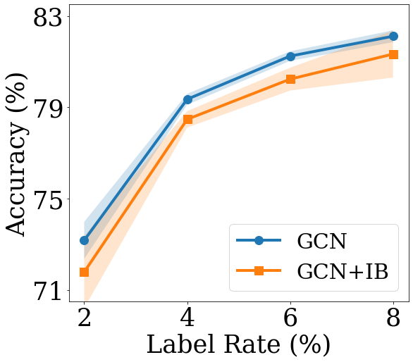
(a) Accuracy

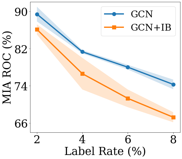
(b) MIA-F ROC

Figure 1. Results of classification and MIA on Cora.

3.6. Impacts of IB to Adversarial Robustness

Intuitively, the negative effects of adversarial perturbations can be reduced with IB, as IB aims to learn representations that only contain information about the label of the classification task. This has been verified by VIB (Alemi et al., 2016), which incorporates IB to deep neural networks on i.i.d data. However, GNNs generally explicitly combine the information of center nodes and their neighbors to obtain node representations. For example, in each layer of GCN, the center node representations are updated by averaging with neighbor representations. Directly using the IB objective function to a GNN encoder may not be sufficient to bottleneck the minimal sufficient neighbor information. As a result, adversarial perturbations on graph structures can still degrade the performance. To empirically verify this, we compare the performance of GCN+IB with GCN on graphs perturbed by Metattack (Zügner and Günnemann, 2019) and Nettack (Zügner et al., 2018). The experimental settings follow the description in Sec. 5.1. The results are shown in Tab. 1. We can observe that the GCN model trained with IB objective function achieves better performance on perturbed graphs, which indicates the potential of giving robust node classification with IB. However, compared with the performance on clean graphs, the accuracy of GCN+IB on perturbed graphs is still relatively poor. This empirically verifies that simply applying IB objective function to the GNN model cannot properly eliminate the noisy information from adversarial edges and there is still a large space to improve IB for robust GNN.

Table 1. Results (Accuracy(%)+std) on perturbed graphs.

Dataset	Model	Clean	Metattack	Netattack
Cora	GCN	73.2 $\pm 0.8$	61.9 $\pm 1.4$	54.6 $\pm 0.8$
	GCN+IB	73.1 $\pm 0.5$	66.3 $\pm 0.3$	58.0 $\pm 1.6$
Citeseer	GCN	72.1 $\pm 0.2$	64.1 $\pm 0.5$	62.3 $\pm 0.7$
	GCN+IB	71.5 $\pm 0.3$	66.8 $\pm 1.1$	63.1 $\pm 1.3$

4. Methodology

As analyzed in Sec. 3.5 and Sec. 3.6, information bottleneck can benefit both robustness and membership privacy. However, there are two challenges to be addressed for achieving better robust and membership privacy-preserving predictions: (i) how to design a graph information bottleneck framework that can handle adversarial edges? and (ii) how to ensure membership privacy with IB given a small set of labels? To address these challenges, we propose a novel framework RM-GIB, which is illustrated in Fig. 2. In RM-GIB, the attribute information and neighbor information are separately bottlenecked. The attribute bottleneck aims to extract node attribute information relevant to the classification. The neighbor bottleneck aims to control the information flow from neighbors to the center node, and to filter out noisy or useless neighbors for the prediction on the center node. Hence, the influence of adversarial edges can be reduced. Moreover, a novel self-supervisor is proposed to guide the training of the neighbor bottleneck to benefit the noisy neighbor elimination. To address the challenge of lacking plenty of labels for membership privacy-preserving, we propose to obtain pseudo labels and combine them with provided labels in the training phase. Specifically, RM-GIB will be trained with the IB objective function with both labels on labeled nodes and pseudo labels on unlabeled nodes to guarantee membership privacy. More details of the design are presented in the following sections.

4.1. Graph Information Bottleneck

In this section, we give the objective of the proposed graph information bottleneck. For graph-structured data, both node attributes and neighbors contain crucial information for node classification. Therefore, for each node $v$, RM-GIB will extract bottleneck code from both node attributes $\mathbf{x}$ and its neighbor set $\mathcal{N}$, which is shown in Fig. 2. More specifically, the bottleneck code is separated into two parts: (i) $\mathbf{z}_{x}=f_{x}(\mathbf{x})$, encoding the node attribute information; (ii) $\mathcal{N}_{S}=f_{n}(\mathcal{N},\mathbf{x})$, a subset of $v$’s neighbors that bottleneck the neighborhood information for prediction. Note that $\mathcal{N}$ can be multi-hop neighbors of a node. With the explicit bottleneck mechanisms on both attributes and neighbors, the noisy information from adversarial perturbations can be suppressed. The objective function of the graph information bottleneck is given as:

(4) $$\min_{\theta}-I(\mathbf{z}_{x},\mathcal{N}_{S};y)+\beta I(\mathbf{z}_{x},\mathcal{N}_{S};\mathbf{x},\mathcal{N})$$

where $\theta$ denotes the learnable parameters of attribute bottleneck and neighbor bottleneck. However, it is challenging to directly optimize Eq.(4) due to the difficulty in computing the mutual information. Thus, we derive tractable variational upper bounds of the two terms in Eq.(4).

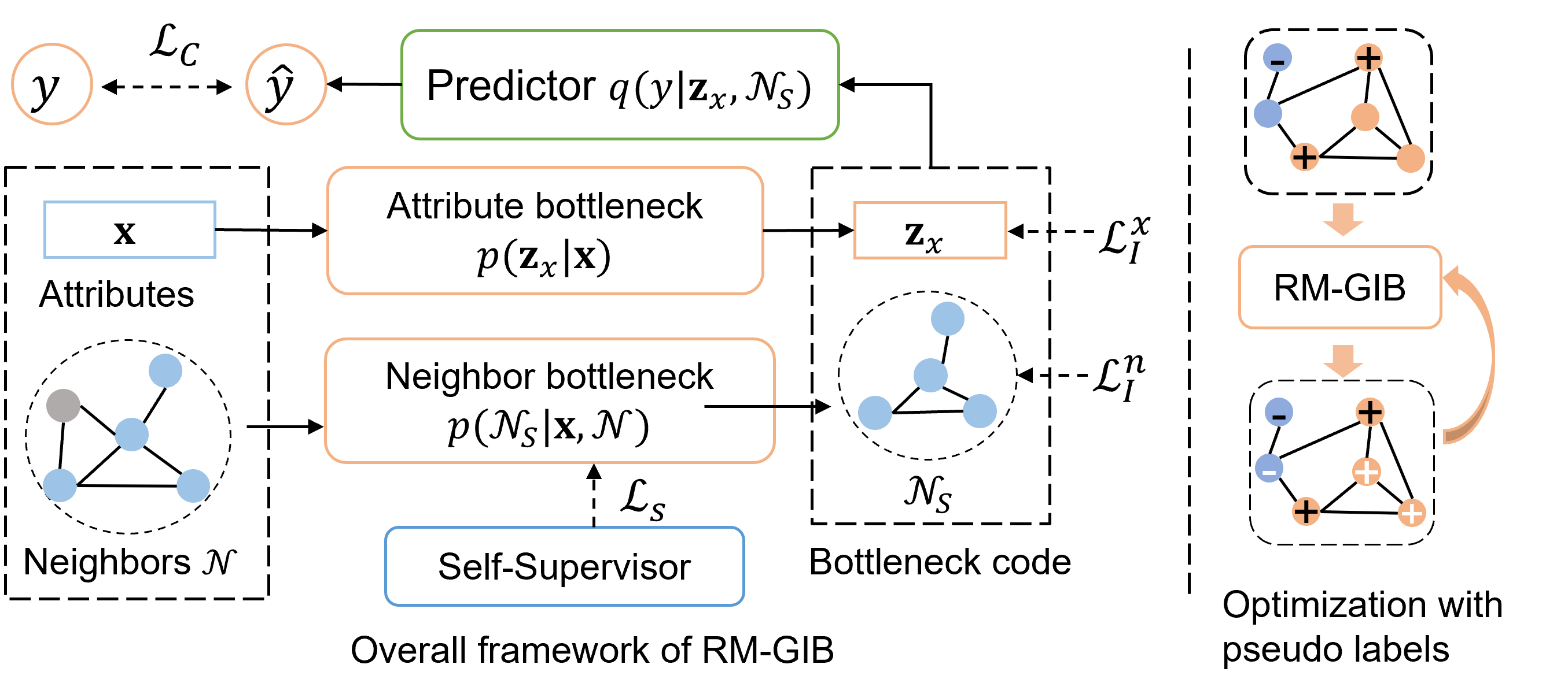
Figure 2. The overall framework of our method and the illustration of optimization with pseudo labels.

Following (Alemi et al., 2016), we introduce $q(y|\mathbf{z}_{x},\mathcal{N}_{S})$ as the parameterized variational approximation of $p(y|\mathbf{z}_{x},\mathcal{N}_{S})$. Note that $q(y|\mathbf{z}_{x},\mathcal{N}_{S})$ also can be viewed as a predictor, which can be flexible to various GNNs. Then, the upper bound of $-I(\mathbf{z}_{x},\mathcal{N}_{S};y)$ can be derived as:

(5) $$-I(\mathbf{z}_{x},\mathcal{N}_{S};y) \leq\mathbb{E}_{p(\mathbf{z}_{x},\mathcal{N}_{S},y)}[-\log q(y|\mathbf{z}_{x},\mathcal{N}_{S})]-H(y)$$

$$\leq\mathbb{E}_{p(\mathbf{z}_{x},\mathcal{N}_{S},y)}[-\log q(y|\mathbf{z}_{x},\mathcal{N}_{S})]=\mathcal{L}_{C}$$

Next, we give the upper bound of the second term in Eq.(4). Since the attribute code $\mathbf{z}_{x}$ is given by $f_{x}(\mathbf{x})$ which only takes node attributes as input, we can infer that $p(\mathbf{z}_{x}|\mathbf{x},\mathcal{N})=p(\mathbf{z}_{x}|\mathbf{x})$. Then, we can get $p(\mathbf{z}_{x},\mathcal{N}_{S}|\mathbf{x},\mathcal{N})=p(\mathbf{z}_{x}|\mathbf{x})p(\mathcal{N}_{S}|\mathbf{x},\mathcal{N})$, which indicates $I(\mathbf{z}_{x},\mathcal{N}_{S}|\mathbf{x},\mathcal{N})=0$. As a result, $I(\mathbf{z}_{x},\mathcal{N}_{S};\mathbf{x},\mathcal{N})$ can be derived to:

(6) $$I(\mathbf{z}_{x},\mathcal{N}_{S};\mathbf{x},\mathcal{N})=I(\mathbf{z}_{x};\mathbf{x},\mathcal{N})+I(\mathcal{N}_{S};\mathbf{x},\mathcal{N}|\mathbf{z}_{x})$$

$$= I(\mathbf{z}_{x};\mathbf{x})+I(\mathcal{N}_{S};\mathbf{x},\mathcal{N})-I(\mathbf{z}_{x};\mathcal{N}_{S})+I(\mathbf{z}_{x},\mathcal{N}_{S}|\mathbf{x},\mathcal{N})$$

$$\leq I(\mathbf{z}_{x};\mathbf{x})+I(\mathcal{N}_{S};\mathbf{x},\mathcal{N})$$

The term $I(\mathbf{z}_{x};\mathbf{x})$ in Eq.(6) can be upper bounded as:

(7) $$I(\mathbf{z}_{x};\mathbf{x})\leq\mathbb{E}_{p(\mathbf{x})}[KL(p(\mathbf{z}_{x}|\mathbf{x})||q(\mathbf{z}_{x}))]=\mathcal{L}_{I}^{x}$$

where $q(\mathbf{z}_{x})$ is the variational approximation to the marginal $p(\mathbf{z}_{x})$ $KL$ denotes the KL divergence. $q(\mathbf{z}_{x})$ is flexible to various distributions such as normal distribution. Similarly, let $q(\mathcal{N}_{S})$ be the variational approximation to the marginal $p(\mathcal{N}_{S})$, the upper bound of $I(\mathcal{N}_{S};\mathbf{x},\mathcal{N})$ is given as:

(8) $$I(\mathcal{N}_{S};\mathbf{x},\mathcal{N})\leq\mathbb{E}_{p(\mathbf{x},\mathcal{N})}[KL(p(\mathcal{N}_{S}|\mathbf{x},\mathcal{N})||q(\mathcal{N}_{S}))]=\mathcal{L}_{I}^{n}$$

With the above derivations, we obtain a variational upper bound of Eq.(4) as the objective function of graph information bottleneck:

(9) $$\min_{\theta}\mathcal{L}_{C}+\beta(\mathcal{L}_{I}^{x}+\mathcal{L}_{I}^{n})$$

where $\theta$ denotes the parameters to be optimized in the graph information bottleneck.

4.2. Neural Network Parameterization

With the objective function of graph information bottleneck given above, we specify the neural network parameterization of the attribute bottleneck $p(\mathbf{z}_{x}|\mathbf{x})$, neighbor bottleneck $p(\mathcal{N}_{S}|\mathbf{x},\mathcal{N})$ and the predictor $q(y|\mathbf{z}_{x},\mathcal{N}_{S})$ in this subsection.

4.2.1. Attribute Bottleneck

The attribute bottleneck aims to learn a code $\mathbf{z}_{x}$ that contains minimal and sufficient information for classification from node attributes $\mathbf{x}$. Inspired by (Alemi et al., 2016), a MLP model and reparameterization trick is adopted to model $p(\mathbf{z}_{x}|\mathbf{x})$ for attribute bottleneck. Specifically, we assume $p(\mathbf{z}_{x}|\mathbf{x})$ follows Gaussian distribution with the mean and variance as the output of a MLP:

(10) $$p(\mathbf{z}_{x}|\mathbf{x})=N(\mathbf{z}_{x};\boldsymbol{\mu},\boldsymbol{\sigma}^{2}\mathbf{I}),\quad\boldsymbol{\mu},\boldsymbol{\sigma}=f_{x}(\mathbf{x})$$

where $f_{x}$ is a MLP which outputs $\boldsymbol{\mu}$ and $\boldsymbol{\sigma}$ as the mean and standard deviation. $\mathbf{z}_{x}$ can be sampled by $\mathbf{z}_{x}=\boldsymbol{\mu}+\boldsymbol{\sigma}\odot\boldsymbol{\epsilon}$, where $\boldsymbol{\epsilon}$ is sampled from the normal distribution $N(\mathbf{0},\mathbf{I})$. As $q(\mathbf{z}_{x})$ is set as normal distribution, $KL(p(\mathbf{z}_{x}|\mathbf{x})||q(\mathbf{z}_{x}))$ can be easily computed for $\mathcal{L}_{I}^{x}$.

4.2.2. Neighbor Bottleneck

For the neighbor bottleneck, it will extract a subset of neighbors that are useful for the target classification task. With an ideal neighbor bottleneck, noisy neighbors caused by adversarial edges and inherent structural noise can be eliminated. Here, we propose a parameterized neighbor bottleneck to model $p(\mathcal{N}_{S}|\mathbf{x},\mathcal{N})$. To ease the difficulty of computation, we decompose $p(\mathcal{N}_{S}|\mathbf{x},\mathcal{N})$ into a multivariate Bernoulli distribution as

(11) $$p(\mathcal{N}_{S}|\mathbf{x},\mathcal{N})={\prod}_{u\in\mathcal{N}_{S}}p_{u}{\prod}_{u\in\mathcal{N}\backslash\mathcal{N}_{S}}(1-p_{u})$$

where $p_{u}$ is the probability of $p(u|\mathbf{x},\mathcal{N})$ that follows Bernoulli distribution. To ensure the gradients can be propagated from the classifier to the neighbor bottleneck module during the optimization, Gumbel-Softmax trick (Jang et al., 2016) with the temperature set as 1 is applied in the sampling phase. Each $p_{u}$ will be estimated by a MLP which takes the center node attributes $\mathbf{x}$ and the attributes of the neighbor $\mathbf{x}_{u}$ as input by:

(12) $$p_{u}=\sigma(\mathbf{h}_{u}^{T}\mathbf{h})\text{ with }~{}~{}\mathbf{h}=f_{n}(\mathbf{x}),~{}~{}\mathbf{h_{u}}=f_{n}(\mathbf{x}_{u}),$$

where $\sigma$ denotes the sigmoid function, and $f_{n}$ denotes a MLP model. As for the variational approximation of marginal distribution $q(\mathcal{N}_{S})$, we also use a multivariate Bernoulli distribution $q(\mathcal{N}_{S})=r^{|\mathcal{N}_{S}|}(1-r)^{|\mathcal{N}|-|\mathcal{N}_{S}|}$ where $r\in[0,1]$ is the probability of a predefined Bernoulli distribution. Then, the information loss on neighbor bottleneck $\mathcal{L}_{I}^{n}$ in Eq.(9) can be computed as:

(13) $$\mathcal{L}_{I}^{n}=\mathbb{E}_{p(\mathbf{x},\mathcal{N})}\big{[}\sum_{u\in\mathcal{N}}p_{u}\log\frac{p_{u}}{r}+(1-p_{u})\log\frac{1-p_{u}}{1-r}\big{]}.$$

4.2.3. Predictor

The predictor $q(y|\mathbf{z}_{x},\mathcal{N}_{S})$ will give predictions based on the bottleneck code of attributes and the extracted subset of neighbors. To fully utilize the rich information from bottlenecked neighbors, a GNN model is deployed as the predictor in RM-GIB. It is flexible to adopt various GNN models such as GCN (Kipf and Welling, 2016) and SGC (Wu et al., 2019a). Note that if $\mathcal{N}_{S}$ contains neighbors in $K$ hops, a $K$ layer GNN will be adopted in this situation. In addition, to avoid the influence of noises in attributes, we also use the attribute bottleneck code $\mathbf{z}_{u}$ for each neighbor $\mathbf{z}_{u}\in\mathcal{N}_{S}$. Let $\mathbf{A}_{S}$ denote the local adjacency matrix that connects nodes in $\mathcal{N}_{S}$ and the center node, the prediction can be formally defined as:

(14) $$\hat{y}=f_{c}(\mathbf{z}_{x},\{\mathbf{z}_{u}\}_{u\in\mathcal{N}_{S}},\mathbf{A}_{S}),$$

where $f_{c}$ is the GNN-based classifier. As the prediction is given on bottlenecked attributes and neighbors, it can give robust predictions against adversarial perturbations on attributes and graph structures.

4.3. Self-supervision for Neighbor Bottleneck

The objective function in Eq.(9) will force the neighbor bottleneck to extract minimal sufficient neighbors that achieve good classification performance. However, the training of neighbor bottleneck will only rely on the implicit supervision from the small set of labels in semi-supervised node classification, which may not be sufficient to train a neighbor bottleneck to handle various structural noises. Therefore, we propose a novel self-supervisor to explicitly guide the training of the neighbor bottleneck. The major intuition is that the neighbor nodes with low mutual information with the center node are likely to be the noisy neighbors that are not helpful for the prediction on the center nodes. Hence, we can first estimate the mutual information of each pair of linked nodes. Then, neighbors with low mutual information scores with the center node can be viewed as negative samples and others as positive samples. Next, we give the details of the mutual information estimation followed by the self-supervision loss on the neighbor bottleneck.

Following (Hjelm et al., 2018), a neural network $f_{M}$ is used to estimate the mutual information between node $v$ and $u$ by:

(15) $$s_{vu}=\sigma({\mathbf{h}_{v}^{m}}^{T}\mathbf{h}_{u}^{m}),~{}~{}\mathbf{h}_{v}^{m}=f_{M}(\mathbf{x}_{v}),~{}~{}\mathbf{h}_{u}^{m}=f_{M}(\mathbf{x}_{u}),$$

where $\sigma$ is the sigmoid activation function and $f_{M}$ is an MLP instead of a GNN model to avoid the negative effects of inherent and adversarial structural noises. A larger $s_{vu}$ indicates higher point-wise mutual information between $v$ and $u$. The mutual information estimator $f_{M}$ can be trained with the following objective (Hjelm et al., 2018):

(16) $$\min_{\theta_{M}}-\frac{1}{|\mathcal{V}|}\sum_{v\in\mathcal{V}}\sum_{u\in\mathcal{N}_{v}}[-\log(s_{vu})-\mathbb{E}_{n\sim p(v)}\log(1-s_{vn})],$$

where $\theta_{M}$ represents parameters of $f_{M}$ and $\mathcal{N}_{v}$ is the set of neighbors of $v$. $p(v)$ is the distribution of sampling negative samples for $v$, which is set as a uniform distribution. With Eq.(16), the mutual information estimator can be trained. Then, we can select the neighbors with a mutual information score lower than the threshold as the negative pairs for neighbor bottleneck. Specifically, for each node $v$, the negative neighbors can be obtained by:

(17) $$\mathcal{N}_{v}^{-}=\{u\in\mathcal{N}_{v};s_{vu}<T\},$$

where $T$ is the predefined threshold. With the negative neighbors, the self-supervision on neighbor bottleneck can be given by:

(18) $$\min_{\theta}\mathcal{L}_{S}=\frac{1}{|\mathcal{V}|}\sum_{v\in\mathcal{V}}\big{[}\sum_{u\in\mathcal{N}_{v}^{+}}-\log(p_{u}^{v})-\sum_{u\in\mathcal{N}_{v}^{-}}\log(1-p_{u}^{v})\big{]},$$

where $\theta$ denotes parameters of RM-GIB, $\mathcal{N}_{v}^{+}=\mathcal{N}_{v}-\mathcal{N}_{v}^{-}$ and $p_{u}^{v}$ corresponds to the probability value of $p(u|\mathbf{x}_{v},\mathcal{N}_{v})$ given by neighbor bottleneck thorough Eq.(12). With Eq.(18), the neighbors who are likely to be noisy will be given lower probability scores in the neighbor bottleneck.

4.4. Privacy-Preserving Optimization with Pseudo Labels

As empirically verified in Sec. 3.5, a large number of labels are required to preserve membership privacy with IB. Thus, we propose to obtain pseudo labels of unlabeled nodes to enlarge the training set to further improve membership privacy. In particular, the adoption of pseudo labels in RM-GIB can benefit the membership privacy in two aspects: (i) classification loss will also be optimized with unlabeled nodes, which increases the confidence scores of prediction on unlabeled nodes. This will make it more difficult to distinguish the prediction vectors of labeled and unlabeled nodes. (ii) involving a large number of unlabeled nodes in the training can improve the generalization ability of attribute and neighbor bottleneck, which can help narrow the gap between the predictions on training samples and test samples. Moreover, the improvement of bottleneck code can also benefit the classification performance. Next, we give the details of the pseudo label collection and the optimization with pseudo labels.

To obtain pseudo labels that are robust to noises in graphs, we can train RM-GIB with the IB objective function combined with the self-supervision on neighbor bottleneck. Let $\mathcal{L}_{C}(\mathcal{V}_{L},\mathcal{Y}_{L})$, $\mathcal{L}_{I}^{x}(\mathcal{V}_{L})$, and $\mathcal{L}_{I}^{n}(\mathcal{V}_{L})$ denote the three terms in the IB objective function in Eq.(9) on the labeled set $\mathcal{V}_{L}$. Then, the process of training RM-GIB for pseudo label collection can be formulated as:

(19) $$\min_{\theta}\mathcal{L}_{C}(\mathcal{V}_{L},\mathcal{Y}_{L})+\beta\big{(}\mathcal{L}_{I}^{x}(\mathcal{V}_{L})+\mathcal{L}_{I}^{n}(\mathcal{V}_{L})\big{)}+\gamma\mathcal{L}_{S},$$

where $\beta$ and $\gamma$ are hyperparameters to control the contributions of regularization on bottleneck code and the self-supervision on neighbor bottleneck. $\theta$ denotes the learnable parameters in RM-GIB. With the RM-GIB trained on Eq.(19), we can collect high-quality pseudo labels $\mathcal{\hat{Y}}_{U}$ of the unlabeled set $\mathcal{V}_{U}$. Then, we combine pseudo labels $\mathcal{\hat{Y}}_{U}$ with provided labels $\mathcal{Y}_{L}$ and retrain RM-GIB for membership privacy-preserving. Let $\mathcal{V}_{P}=\mathcal{V}_{L}\cup\mathcal{V}_{U}$ and $\mathcal{\hat{Y}}_{P}=\mathcal{\hat{Y}}_{U}\cup\mathcal{Y}_{L}$ denote the enlarged labeled node set and labels, the membership privacy-preserving optimization can be formally written as:

(20) $$\min_{\theta}\mathcal{L}_{C}(\mathcal{V}_{P},\mathcal{\hat{Y}}_{P})+\beta(\mathcal{L}_{I}^{x}(\mathcal{V}_{P})+\mathcal{L}_{I}^{n}(\mathcal{V}_{P}))+\gamma\mathcal{L}_{S}$$

The hyperparameters $\beta$ and $\gamma$ are set the same as Eq.(19).

Table 2. Statistics of datasets.

	Cora	Citeseer	Pubmed	Flickr
#classes	7	6	3	7
#features	1,433	3,703	500	500
#nodes	2,485	2,110	19,717	89,250
#edges	5,069	3,668	44,338	899,756

Table 3. Comparison with baselines in defending membership inference attack on various clean graphs.

Dataset	Metrics	GCN	GCN+PL	Adv-Reg	DP-SGD	GIB	LBP	NSD	RM-GIB
Cora	Accuracy (%) $\uparrow$	73.2$\pm 0.8$	74.7$\pm 0.2$	75.5 $\pm 0.8$	57.9 $\pm 0.2$	72.5 $\pm 0.7$	69.7 $\pm 0.7$	65.4 $\pm 0.3$	78.1 $\bf\pm 0.4$
	MIA-F ROC (%) $\downarrow$	90.6 $\pm 0.8$	61.6$\pm 0.2$	70.6 $\pm 0.4$	73.8 $\pm 3.3$	86.6 $\pm 0.8$	71.0 $\pm 1.7$	81.8 $\pm 0.8$	57.4 $\bf\pm 0.2$
	MIA-S ROC (%) $\downarrow$	88.8 $\pm 0.2$	63.8 $\pm 0.8$	70.6 $\pm 0.3$	75.3 $\pm 1.2$	87.3 $\pm 0.7$	71.1 $\pm 1.5$	81.2 $\pm 0.6$	59.5 $\bf\pm 1.2$
Citeseer	Accuracy (%)$\uparrow$	72.1 $\pm 0.2$	73.1 $\pm 0.2$	72.4 $\pm 1.0$	57.9 $\pm 0.2$	71.0 $\pm 0.2$	66.5 $\pm 0.8$	65.6 $\pm 0.2$	73.9 $\bf\pm 0.6$
	MIA-F ROC (%)$\downarrow$	88.5 $\pm 1.8$	65.2 $\pm 0.6$	60.9 $\pm 0.6$	73.8 $\pm 3.3$	85.8 $\pm 0.5$	66.6 $\pm 0.4$	84.4 $\pm 0.1$	55.2 $\bf\pm 0.8$
	MIA-S ROC (%)$\downarrow$	84.9 $\pm 1.5$	65.8 $\pm 0.5$	61.2 $\pm 1.1$	75.3 $\pm 1.2$	80.3 $\pm 0.4$	67.3 $\pm 0.7$	88.3 $\pm 0.1$	55.9 $\bf\pm 1.7$
Pubmed	Accuracy (%)$\uparrow$	79.9 $\pm 0.1$	79.9 $\pm 0.1$	79.4 $\pm 1.1$	69.3 $\pm 3.2$	78.1 $\pm 0.4$	78.3 $\pm 0.1$	75.5 $\pm 0.1$	81.4 $\bf\pm 0.2$
	MIA-F ROC (%)$\downarrow$	75.1 $\pm 0.2$	60.8 $\pm 0.2$	60.6 $\pm 1.8$	56.3 $\pm 1.8$	68.5 $\pm 1.6$	67.4 $\pm 1.6$	68.4 $\pm 0.2$	53.9 $\bf\pm 0.3$
	MIA-S ROC (%)$\downarrow$	73.4 $\pm 0.1$	63.4 $\pm 0.2$	62.8 $\pm 2.0$	58.3 $\pm 2.1$	67.0 $\pm 1.8$	65.7 $\pm 2.0$	72.1 $\pm 0.1$	57.2 $\bf\pm 0.2$
Flickr	Accuracy (%)$\uparrow$	52.5 $\bf\pm 0.2$	51.8 $\pm 0.8$	48.2 $\pm 1.8$	46.2 $\pm 0.1$	45.2 $\pm 2.0$	44.6 $\pm 0.5$	41.6 $\pm 0.5$	52.2 $\pm 0.2$
	MIA-F ROC (%)$\downarrow$	87.9 $\pm 0.7$	72.9 $\pm 1.5$	64.3 $\pm 3.9$	66.5 $\pm 0.7$	79.9 $\pm 4.4$	67.9 $\pm 0.8$	59.0 $\pm 1.5$	58.2 $\bf\pm 0.1$
	MIA-S ROC (%)$\downarrow$	84.2 $\pm 0.7$	69.7 $\pm 1.2$	66.4 $\pm 1.2$	65.1 $\pm 0.6$	76.5 $\pm 0.7$	71.3 $\pm 0.9$	63.5 $\pm 1.3$	57.6 $\bf\pm 0.3$

5. Experiments

In this subsection, we evaluate the proposed RM-GIB on various real-world datasets to answer the following research questions:

• RQ1 Can our proposed RM-GIB preserve the membership privacy in node classification given a small set of labeled nodes?

• RQ2 Is RM-GIB robust to adversarial perturbations on graphs and can membership privacy be simultaneously guaranteed?

• RQ3 How does each component of RM-GIB contribute to the robustness and membership privacy?

5.1. Experimental Settings

5.1.1. Datasets

We conduct experiments on widely used publicly available benchmark datasets, i.e., Cora, Citeseer, Pubmed (Kipf and Welling, 2016), and Flickr (Zeng et al., 2020). The key statistics of these datasets can be found in Tab. 2. Details of the dataset settings can be found in Appendix A

5.1.2. Baselines

To evaluate the performance in preserving membership privacy, we compare RM-GIB with the representative graph neural network GCN (Kipf and Welling, 2016) and an existing work of graph information bottleneck GIB (Wu et al., 2020). We also incorporate a state-of-the-art regularization method, i.e., adversarial regularization (Nasr et al., 2018) (Adv-Reg). A differential privacy-based method DP-SGD (Abadi et al., 2016) is also compared. Additionally, we compare two recent methods for defending membership inference attacks on GNNs, which are LBP (Olatunji et al., 2021) and NSD (Olatunji et al., 2021). LBP adds noise to the posterior before it is released to end users. NSD randomly chooses neighbors of the queried node to limit the amount of information used in the target model for membership privacy protection.

To evaluate the robustness of RM-GIB against adversarial attacks on graphs, apart from GCN and GIB, we also compare representative and state-of-the-art robust GNNs. Specifically, we compare two classical preprocessing methods, i.e., GCN-jaccard (Wu et al., 2019b) and GCN-SVD (Entezari et al., 2020). Two state-of-the-art robust GNNs are also incorporated in the comparison, which are Elastic (Liu et al., 2021) and RSGNN (Dai et al., 2022a). For more detailed descriptions about the above baselines, please refer to Appendix B. To make a fair comparison, the hyperparameters of all baselines are tuned based on the validation set. For our RM-GIB, hyperparameter sensitivity analysis is given in Sec. 5.5. More implementation details of RM-GIB can be found in Appendix C.

5.1.3. Evaluation Protocol

In this subsection, we provide details of experimental settings and metrics to evaluate the performance in defending membership inference attacks and adversarial attacks.

Membership Privacy. We adopt the state-of-the-art MIA on GNNs in (Olatunji et al., 2021) for membership privacy-preserving evaluation. The shadow training  (Olatunji et al., 2021) described in Sec. 3.2 is adopted. Here, GCN is applied as the shadow model. The attack setting is set as black-box, i.e., the attacker can only obtain the predictive vectors and cannot access model parameters. As for the shadow dataset, we use two settings:

• MIA-F: The attacker has the complete graph used for training along with a small set of labels;

• MIA-S: The attacker has a subgraph of the dataset with a small set of labels; In all experiments, we randomly sample 50% nodes as the subgraph that is available for the attacker.

In both settings, the labeled nodes used in the attack have no overlap with the training set of target model. The number of labeled nodes used in the attack is the same as the training set. The attack ROC score is used as a metric for membership privacy-preserving evaluation. And a GNN model with a lower attack ROC score indicates better performance in defending MIAs.

Robustness. To evaluate the robustness against adversarial attacks, we evaluate RM-GIB on graphs perturbed by following methods:

• Mettack (Zügner and Günnemann, 2019): It aims to reduce the overall performance of the target GNN by perturbing attributes and graph structures. The perturbation rate is set as 0.2 in all experiments.

• Nettack (Zügner et al., 2018): It aims to lead the GNN to misclassify target nodes. Following (Dai et al., 2022a), 15% nodes are randomly selected as target nodes.

As the cited papers do, both Mettack and Nettack can access the whole graph. Similar to MIA, the adversarial attacker is assumed to have nodes with labels that do not overlap with the training set.

5.2. Privacy Preserving on Clean Graphs

To answer RQ1, we compare RM-GIB with baselines in defending membership inference attacks on various real-world graphs. The prediction accuracy of each method is reported. As described in Sec. 5.1.3, for membership privacy-preserving evaluation, we report the membership attack ROC score on two different settings, i.e., MIA-F and MIA-S, which correspond to the MIA-F ROC and MIA-S ROC in the evaluation metrics. Note that lower attack ROC score indicates better performance in preserving privacy. The results on the default dataset split setting described in Appendix A are reported in Tab. 3. Results on different sizes of training set can be found in Appendix 6. From the Tab. 3, we can observe:

• GCN can be easily attacked by membership inference attacks. This demonstrates the necessity of developing membership privacy-preserving methods for node classification on graphs.

• RM-GIB gives significantly lower scores in MIA-F ROC and MIA-S ROC than baselines. The attack ROC scores can be even close to 0.5, indicating invalid privacy attacks. This demonstrates the effectiveness of RM-GIB in preserving membership privacy.

• The baseline methods often improve membership privacy with a significant decline in accuracy. By contrast, our RM-GIB can simultaneously maintain high prediction accuracy and preserve membership privacy. This is because baselines generally need to either largely regularize the model or inject strong noises. RM-GIB does not only rely on the regularization in the IB objective function. Pseudo labels are further incorporated in training RM-GIB, which helps to bottleneck redundant information to improve performance and narrow the gap between training and test samples for preserving membership privacy.

Table 4. Comparison with Robust GNNs in node classification (Accuracy(%)$\pm$Std) on various adversarially perturbed graphs.

Dataset	Graph	GCN	GIB	GCN-jaccard	GCN-SVD	Elastic	RSGNN	RM-GIB
Cora	Clean	73.2 $\pm 0.8$	72.5 $\pm 0.7$	68.9 $\pm 0.6$	65.1 $\pm 0.6$	77.9 $\pm 0.9$	74.6 $\pm 1.0$	78.5 $\bf\pm 0.6$
	Metattack	61.9 $\pm 1.4$	65.6 $\pm 0.1$	64.4 $\pm 0.2$	60.5 $\pm 1.3$	70.2 $\pm 0.4$	65.3 $\pm 2.5$	71.1 $\bf\pm 0.6$
	Nettack	54.6 $\pm 0.8$	60.1 $\pm 3.2$	58.6 $\pm 0.5$	54.8 $\pm 0.7$	64.8 $\pm 1.1$	66.9 $\bf\pm 0.4$	65.6 $\pm 1.3$
Citeseer	Clean	72.1 $\pm 0.2$	71.0 $\pm 0.2$	72.2 $\pm 0.1$	63.0 $\pm 0.4$	73.7 $\pm 0.3$	73.7 $\pm 1.3$	73.9 $\bf\pm 0.6$
	Metattack	64.1 $\pm 0.5$	66.8 $\pm 0.7$	70.5 $\pm 0.1$	59.7 $\pm 1.1$	71.5 $\pm 0.4$	73.0 $\bf\pm 0.3$	72.1 $\pm 0.9$
	Nettack	62.3 $\pm 0.7$	63.8 $\pm 1.6$	68.9 $\pm 0.2$	55.6 $\pm 1.1$	68.5 $\pm 0.2$	69.0 $\pm 0.9$	69.9 $\bf\pm 0.8$
Pubmed	Clean	79.8 $\pm 0.1$	78.1 $\pm 0.4$	79.5 $\pm 0.1$	75.1 $\pm 0.1$	80.6 $\pm 0.2$	75.6 $\pm 0.3$	81.4 $\bf\pm 0.1$
	Metattack	67.5 $\pm 0.1$	61.5 $\pm 0.4$	74.1 $\pm 0.6$	74.5 $\pm 0.1$	73.5 $\pm 0.2$	74.4 $\pm 0.2$	77.3 $\bf\pm 0.1$
	Nettack	68.2 $\pm 0.1$	67.5 $\pm 0.6$	74.0 $\pm 0.7$	67.9 $\pm 0.2$	73.2 $\pm 0.3$	72.8 $\pm 0.6$	75.0 $\bf\pm 0.2$

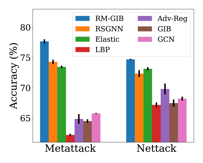
(a) Accuracy on Pubmed

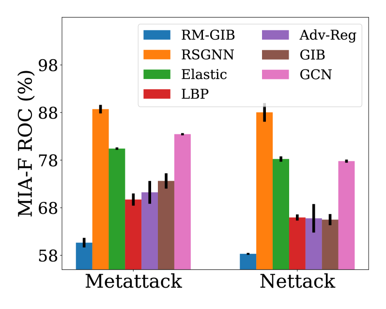
(b) MIA-F ROC on Pubmed

Figure 3. Results on perturbed Cora and Pubmed graphs.

5.3. Results on Adverarially Perturbed Graphs

To answer RQ2, we first compare RM-GIB with Robust GNNs on various perturbed graphs. Then, the performance of membership privacy-preserving on perturbed graphs is also evaluated.

5.3.1. Robust Classification

Two types of adversarial attacks, i.e., Metattack and Nettack, are considered for all datasets. Metattack and Nettack will result in out of memory in attacking the large-scale dataset Flickr. Therefore, we only conduct experiments on Cora, Citeseer, and Pubmed. The detailed settings of attacks follow the description in Sec. 5.1. The average results and standard deviations of 5 runs are reported in Tab. 4, where we can observe:

• Our proposed RM-GIB achieves comparable/better results compared with the state-of-the-art robust GNNs on perturbed graphs, which indicates RM-GIB can mitigate the attribute noises and structural noises with the attribute and neighbor bottleneck.

• Our RM-GIB performs much better than GIB, which also applies IB on graphs to filter out noises in attributes and structures. This is because self-supervision on neighbor bottleneck is adopted in RM-GIB to eliminate noisy neighbors irrelevant to label information. Meanwhile, incorporating pseudo labels of unlabeled nodes also benefits bottleneck code learning.

• On clean graphs, RM-GIB can also consistently outperform baselines including GCN. This is because clean graphs can contain superfluous information and inherent noises, which can be alleviated with the bottleneck in RM-GIB.

5.3.2. Membership Privacy Preserving

We also evaluate RM-GIB on perturbed graphs in terms of membership privacy-preserving. The most effective privacy-preserving baselines in Tab. 3 and robust GNNs in Tab. 4 are selected for comparison. The accuracy and MIA-F ROC on Pubmed and Cora that are perturbed by Metattack and Nettack are shown in Fig. 3 and Fig. 6, respectively. From this figure, we can find that robust GNNs generally fail in preserving privacy. And privacy-preserving baselines give poor classification performance on perturbed graphs. In contrast, RM-GIB can simultaneously preserve membership privacy and give robust predictions in a unified framework.

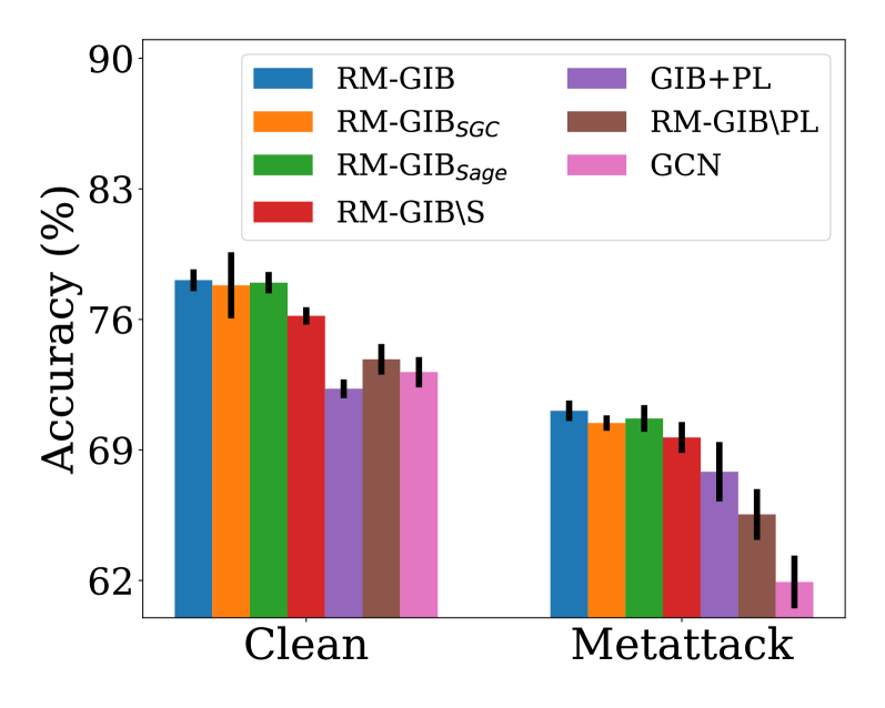
(a) Accuracy

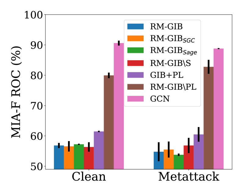
(b) MIA-F ROC

Figure 4. Ablation studies on the Cora graph.

5.4. Ablation Study

To answer RQ3, we conduct an ablation study to understand the effects of the proposed graph information bottleneck, self-supervision on the neighbor bottleneck, and adoption of pseudo labels. To demonstrate the effectiveness of the self-supervision on the neighbor bottleneck, we set $\gamma$ as 0 when we train RM-GIB and denote this variant as RM-GIB$\backslash$S. Moreover, to show our RM-GIB can better bottleneck noisy neighbors, a GIB+PL model which trains GIB (Wu et al., 2020) with pseudo labeling is adopted as a reference. We train a variant RM-GIB$\backslash$PL that does not incorporate any pseudo labels of unlabeled nodes in the optimization to show the benefits of using pseudo labels in the training. To prove the flexibility of RM-GIB, we train two variants of RM-GIB that use SGC and GraphSage as the predictor, which correspond to RM-GIB_SGC and RM-GIB_Sage. Results of classification and membership privacy-preserving on clean graphs and Metattack perturbed graphs are reported in Fig. 4. We only show results on Cora as we have similar observations on other datasets. Concretely, we observe that:

• RM-GIB_SGC and RM-GIB_Sage achieve comparable results in both robustness and membership privacy-preserving, which shows the flexibility of our proposed RM-GIB.

• The accuracy of RM-GIB$\backslash$S and GIB+PL is worse than RM-GIB especially on perturbed graphs, which verifies self-supervision on neighbor bottleneck can benefit filtering out noisy neighbors.

• RM-GIB outperforms RM-GIB$\backslash$PL in both accuracy and membership privacy preserving. This shows the effectiveness of adopting pseudo labels to IB for preserving membership privacy. Pseudo labels on unlabeled nodes also improve the quality of the bottleneck code, resulting in better classification performance.

5.5. Hyperparameter Sensitivity Analysis

In this subsection, we conduct hyperparameter sensitivity analysis to investigate how $\beta$ and $\gamma$ affect the RM-GIB, where $\beta$ controls the regularization on the bottleneck code and $\gamma$ controls the contributions of self-supervision on the neighbor bottleneck. More specifically, we vary $\beta$ and $\gamma$ as $\{0.0003,0.0001,0.003,0.001,0.03,0.1\}$ and $\{0.00001,0.0001,0.001,0.01,0.1\}$, respectively. We report the accuracy and MIA-F ROC on Cora graph perturbed by Metattack. Similar trends are also observed on other datasets and attack methods. The results are shown in Fig. 5. We find that: (i) With the increase of $\beta$, the performance of classification and membership privacy-preserving both become better. This is because with very small $\beta$, the regularization will be too weak, which can cause overfitting and failure in filtering out noisy information. When $\beta$ is very large, the strong constraint will lead to poor generalization ability of bottleneck code, resulting in worse performance of both classification and membership privacy; (ii) With the increment of $\gamma$, the classification accuracy on perturbed graphs tends to first increase and decrease. And its effects on preserving membership privacy is negligible. When $\gamma$ is in $[0.0001,0.001]$, RM-GIB generally gives good classification performance.

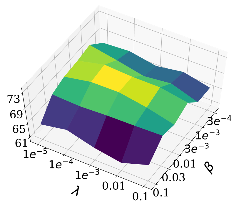
(a) Accuracy

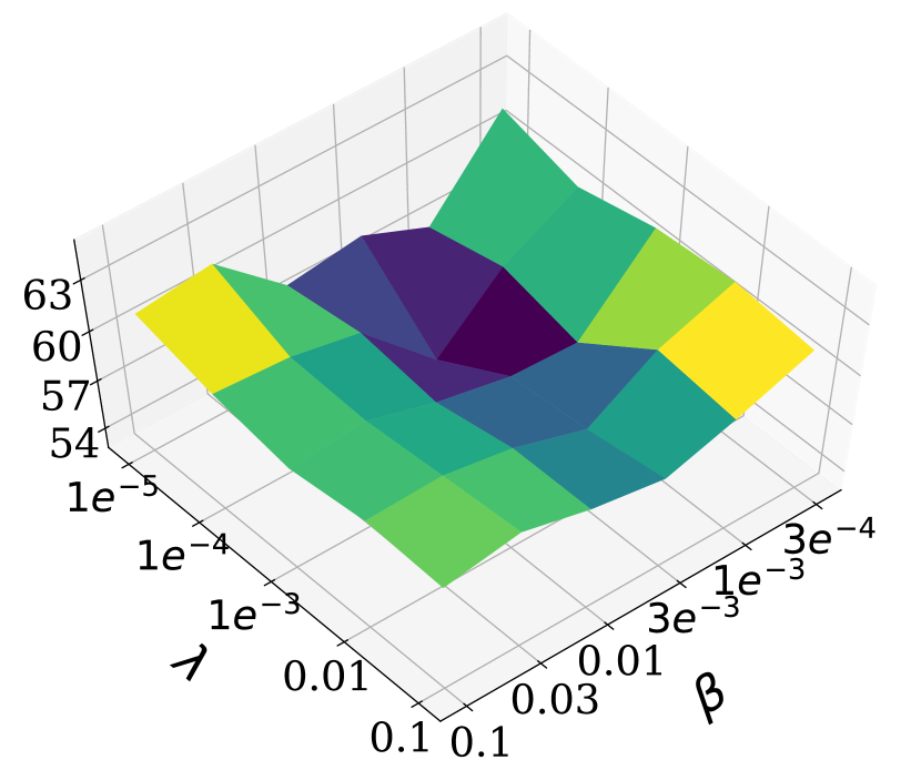
(b) MIA-F ROC

Figure 5. Hyperparameter analysis on the perturbed Cora.

6. Conclusion And Future Work

In this paper, we study a novel problem of developing a unified framework that can simultaneously achieve robustness and preserve membership privacy. We verify that IB has potential to eliminate the noises and adversarial perturbations in the data. In addition, IB regularizes the predictions on labeled samples, which can benefit membership privacy. However, the deployment of IB on graph-structured data is challenged by structural noises and shortage of labels in node classification on graphs. To address these issues, we propose a novel graph information bottleneck framework that separately bottlenecks the attribute and neighbor information to handle attribute and structural noises. A self-supervision loss is applied to neighbor bottleneck to further help to filter out adversarial edges and inherent structural noises. Moreover, pseudo labels of unlabeled nodes are incorporated in optimization with pseudo labels to enhance membership privacy. There are two directions that need further investigation. In this work, we only focus on membership inference attacks. We will investigate whether IB can help defend against other privacy attacks such as attribute inference attacks. Since IB can extract minimal sufficient information, it would be interesting to investigate whether the sensitive information of users such as race can be removed for fairness.

7. Acknowledgement

This material is based upon work partially supported by National Science Foundation (NSF) under grant number IIS-1909702 and the Army Research Office (ARO) under grant number W911NF21-1-0198 to Suhang Wang. The findings and conclusions in this paper do not necessarily reflect the view of the funding agency.

Appendix A Dataset

Cora, Citeseer, and Pubmed are citation networks, where nodes in the graphs represent the papers and edges denote citation relationship. The attributes of the nodes are the bag-of-words of these papers. For small citation graphs, i.e., Cora and Citeseer, we randomly sample 2% nodes as the training set. For the large citation graph Pubmed, we randomly sample 0.5% nodes as the training set. As for Flickr (Zeng et al., 2020), it is a large-scale graph to categorize the type of images. Each node represents an image and the image description is used as a node attribute. Edges are formed between nodes sharing common properties. We randomly sample 2% nodes from Flickr as the training set. Splits of validation and test sets on all datasets follow the cited papers for consistency. Note that the training node set doesn’t overlap with the validation and test sets.

Appendix B Baselines

To evaluate the performance in preserving membership privacy, we compare RM-GIB with the following representative and state-of-the-art methods in defending membership inference attacks:

• GCN (Kipf and Welling, 2016): This is a representative graph convolutional network which defines graph convolution with spectral analysis.

• GCN+PL (Lee et al., 2013): A GCN is firstly trained to obtain pseudo labels. Then, pseudo labels of unlabeled nodes and labels of labeled nodes are used to retrain the GCN.

• GIB (Wu et al., 2020): It proposes a graph information bottleneck that regularizes the structural and attribute information in GAT (Veličković et al., 2018).

• Adv-Reg (Nasr et al., 2018): Min-max game between the training model and the membership inference attacker is introduced as regularization for membership privacy-preserving.

• DP-SGD (Abadi et al., 2016): This is a differentially private mechanism that adds noises to gradients during optimization for preserving privacy.

• LBP (Olatunji et al., 2021): This is an output perturbation method by adding noise to the posterior before it is released to end users.

• NSD (Olatunji et al., 2021): It randomly chooses neighbors of the queried node in inference to limit the amount of information used in the target model for membership privacy protection.

Apart from GCN and GIB, we also compare the following representative and state-of-the-art robust GNNs to evaluate the robustness of RM-GIB against adversarial attacks on graphs:

• GCN-jaccard (Wu et al., 2019b): It preprocesses a graph by removing edges linking nodes with low Jaccard feature similarity, then trains a GCN on the preprocessed graph.

• GCN-SVD (Entezari et al., 2020): It uses a low-rank approximation of the perturbed graph to defend against graph adversarial attacks with the observation that adversarial edges often result in a high-rank adjacency matrix.

• Elastic (Liu et al., 2021): Elastic designs a robust message-passing mechanism which incorporates $l_{1}$-based graph smoothing in GNNs.

• RSGNN (Dai et al., 2022a): This is a state-of-the-art robust GNN that denoises and densifies the noisy graph to give robust predictions.

Table 5. Results of defending membership inference attack (Accuracy(%)$\uparrow$ — MIA-F ROC(%) $\downarrow$) with various label rates.

Dataset	Method	2%	4%	6%	8%
Cora	GCN	73.2$\pm$0.8 — 89.4$\pm$0.5	79.4$\pm$0.2 — 81.3$\pm$1.4	81.2$\pm$0.2 — 78.0$\pm$0.4	82.1$\pm$0.3 — 74.3$\pm$0.1
	GIB	72.5$\pm$0.7 — 86.6$\pm$0.8	78.8$\pm$0.5 — 78.6$\pm$0.7	80.6$\pm$1.5 — 71.4$\pm$1.8	80.9$\pm$0.8 — 67.8$\pm$0.6
	RM-GIB	78.5$\pm$0.6 — 56.4$\pm$0.2	79.6$\pm$0.6 — 56.9$\pm$0.3	81.9$\pm$0.4 — 55.9$\pm$0.6	81.9$\pm$0.3 — 54.4$\pm$1.0
Citeseer	GCN	70.2$\pm$0.2 — 88.5$\pm$1.8	71.3$\pm$0.4 — 83.1$\pm$0.3	73.6$\pm$0.1 — 76.0$\pm$0.3	73.9$\pm$0.1 — 73.2$\pm$0.1
	GIB	70.1$\pm$1.1 — 87.4$\pm$0.6	72.1$\pm$0.6 — 80.4$\pm$2.1	74.8$\pm$0.5 — 70.9$\pm$0.3	74.6$\pm$0.7 — 69.9$\pm$0.9
	RM-GIB	73.9$\pm$0.6 — 55.2$\pm$0.8	73.6$\pm$0.8 — 53.0$\pm$0.1	76.1$\pm$0.3 — 50.3$\pm$0.7	76.4$\pm$0.7 — 50.2$\pm$1.8
Pubmed	GCN	81.0$\pm$0.1 — 56.6$\pm$0.1	82.8$\pm$0.4 — 56.6$\pm$0.1	83.9$\pm$0.1 — 54.9$\pm$0.1	85.3$\pm$0.1 — 53.0$\pm$0.1
	GIB	81.9$\pm$0.1 — 56.1$\pm$0.2	84.0$\pm$0.2 — 53.7$\pm$0.4	85.1$\pm$0.3 — 52.0$\pm$0.1	85.5$\pm$0.8 — 51.3$\pm$0.1
	RM-GIB	84.0$\pm$0.1 — 50.3$\pm$0.5	85.2$\pm$0.4 — 49.8$\pm$0.7	85.9$\pm$0.3 — 50.1$\pm$0.3	86.4$\pm$0.2 — 50.1$\pm$0.1

Appendix C Implementation Details

A 2-layer MLP is deployed as the attribute bottleneck. The neighbor bottleneck also uses a 2-layer MLP. As for the predictor, we use a 2-layer GCN without on default. The mutual information estimator used for self-supervision on neighbor bottleneck also deploys a 2-layer MLP. All the hidden dimensions of the neural networks are set as 256. For the hyperparameter $T$ which is the threshold to determine the negative neighbors for self-supervision, it is set as 0.5 for all experiments. As for the hyperparameters $\beta$ and $\gamma$ used in the final objective function Eq.(20), they are selected based on accuracy on the validation set with grid search. Specifically, we vary $\beta$ and $\gamma$ as $\{0.0003,0.0001,0.003,0.001,0.03,0.1\}$ and $\{0.00001,0.0001,0.001,0.01,0.1\}$, respectively.

Appendix D Proof Details

Recall that in IB, for a given training sample $(\mathbf{x}_{n},y_{n})$, its distribution of $\mathbf{z}$ is obtained by $P(\mathbf{z}|\mathbf{x}_{n},y_{n};\theta)=f_{\theta}(\mathbf{z},\mathbf{x}_{n})$, where $f_{\theta}(\mathbf{z},\mathbf{x}_{n})$ is the probability density function modeled by the nerual network with parameters $\theta$. In the practice of computing mutual information, $P(\mathbf{x},y,\mathbf{z};\theta)$ is approximated with the empirical data distribution $P(\mathbf{x},y,\mathbf{z};\theta)=\frac{1}{N}\sum_{n=1}^{N}\delta_{\mathbf{x}_{n}}(\mathbf{x})\delta_{y_{n}}(y)f_{\theta}(\mathbf{z},\mathbf{x}_{n})$, where $\delta()$ is the Dirac function. Then, we can have the following equations:

(21) $$P(\mathbf{x},\mathbf{z};\theta)=\int_{y}P(\mathbf{x},y,\mathbf{z};\theta)dY=\frac{1}{N}\sum_{n=1}^{N}\delta_{\mathbf{x}_{n}}(\mathbf{x})f_{\theta}(\mathbf{z},\mathbf{x}_{n})$$

(22) $$P(\mathbf{x},y;\theta)=\int_{\mathbf{z}}P(\mathbf{x},y,\mathbf{z};\theta)d\mathbf{z}=\frac{1}{N}\sum_{n=1}^{N}\delta_{\mathbf{x}_{n}}(\mathbf{x})\delta_{y_{n}}(y)$$

(23) $$P(\mathbf{x};\theta)=\int_{y}P(\mathbf{x},y;\theta)d\mathbf{x}=\frac{1}{N}\sum_{n=1}^{N}\delta_{\mathbf{x}_{n}}(\mathbf{x})$$

The $I_{\theta}(\mathbf{z};y|\mathbf{x})$ can be computed by:

(24) $$I_{\theta}(\mathbf{z};y|\mathbf{x})$$

$$=\int_{\mathbf{x}}\int_{y}\int_{\mathbf{z}}p(\mathbf{x},y,\mathbf{z};\theta)\log\frac{P(\mathbf{x};\theta)P(\mathbf{x},y,\mathbf{z};\theta)}{P(\mathbf{x},y;\theta)P(\mathbf{x},\mathbf{z};\theta)}d\mathbf{x}dyd\mathbf{z}$$

$$=\frac{1}{N}\int_{\mathbf{x}}\int_{y}\int_{\mathbf{z}}\Big{(}\sum_{n=1}^{N}\delta_{\mathbf{x}_{n}}(\mathbf{x})\delta_{y_{n}}(y)f_{\theta}(\mathbf{z},\mathbf{x}_{n})\Big{)}$$

$$\cdot\log\frac{\big{(}\sum_{n=1}^{N}\delta_{\mathbf{x}_{n}}(\mathbf{x})\big{)}\cdot\big{(}\sum_{n=1}^{N}\delta_{\mathbf{x}_{n}}(\mathbf{x})\delta_{y_{n}}(y)f_{\theta}(\mathbf{z},\mathbf{x}_{n})\big{)}}{\big{(}\sum_{n=1}^{N}\delta_{\mathbf{x}_{n}}(\mathbf{x})\delta_{y_{n}}(y)\big{)}\cdot\big{(}\sum_{n=1}^{N}\delta_{\mathbf{x}_{n}}(\mathbf{x})f_{\theta}(\mathbf{z},\mathbf{x}_{n})\big{)}}d\mathbf{x}dyd\mathbf{z}$$

$$=\frac{1}{N}\int_{\mathbf{z}}\sum_{n=1}^{N}f_{\theta}(\mathbf{z},\mathbf{x}_{n})\log\frac{f_{\theta}(\mathbf{z},\mathbf{x}_{n})}{f_{\theta}(\mathbf{z},\mathbf{x}_{n})}=0$$

Based on the above proof, we verify that $I_{\theta}(\mathbf{z};y|\mathbf{x})=0$ regardless the value of model parameters. Thus, we can derive the first line of Eq.(3) in our paper.

Appendix E Time Complexity Analysis

We analyze the time complexity of the proposed RM-GIB in the following. The time complexity mainly comes from the pretraining of self-supervisor for the neighbor bottleneck, and the training of RM-GIB. Let $h$ and $K$ denote the embedding dimension and training epochs, respectively. The cost of training the self-supervisor is approximately $O(Khd|\mathcal{V}|)$, where $d$ is the average degree of nodes and $|\mathcal{V}|$ is the number of nodes in the graph. Next, we analyze the time complexity of the optimization of RM-GIB. The time complexity of attribute bottleneck and neighbor bottleneck in each epoch are $O(h|\mathcal{V}|)$ and $O(hd|\mathcal{V}|)$, respectively. As for the computation cost of the predictor is approximately $O(hd|\mathcal{V}|)$ in each epoch. The privacy-preserving optimization requires firstly training RM-GIB for pseudo label collection followed by the optimization on the enlarged label set. Hence, the time complexity of optimizing RM-GIB is $O(2Kh(2d+1)|\mathcal{V}|)$. Combining the training of self-supervisor, the overall time complexity for training is $O(Kh(4d+3)|\mathcal{V}|)$. Our RM-GIB is linear to the size of the graph, which proves its scalability.

Appendix F Additional Experimental Results

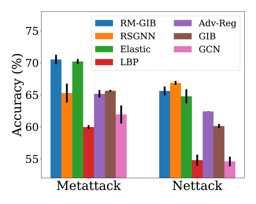
(a) Accuracy on Cora

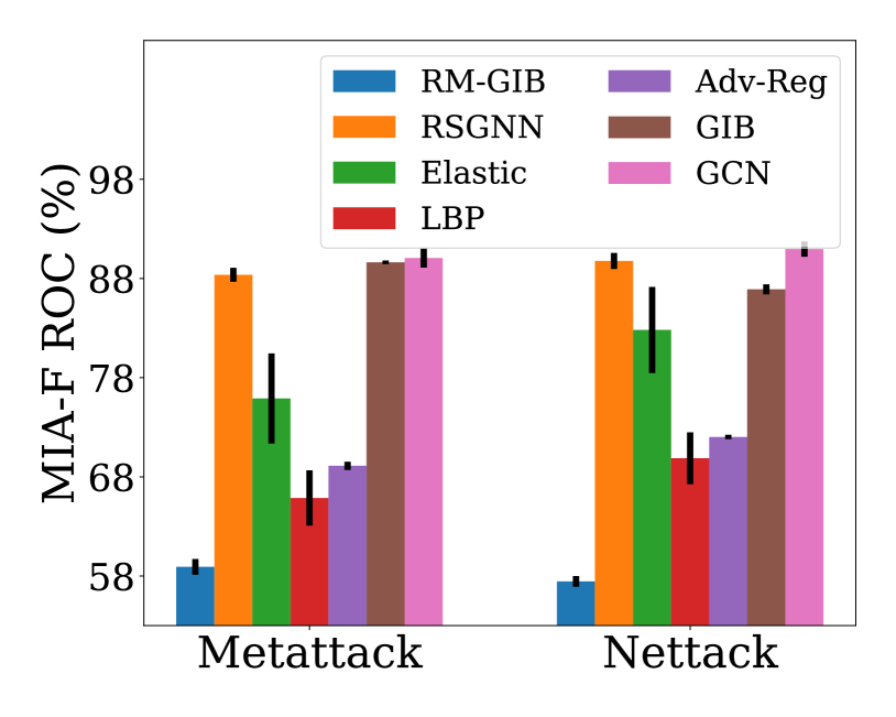
(b) MIA-F ROC on Cora

Figure 6. Additional results on the perturbed Cora.

The additional results on the perturbed Cora graph are shown in Fig. 6, which have the same observations as Fig. 3.

Impacts of Label Rates. We add the experiments that vary label rates by {2%, 4%, 6%, 8%} to verify our motivation and the effectiveness of our RM-GIB. All the hyperparameters of GCN, GIB, and our RM-GIB are tuned on the validation set for a fair comparison. The results are presented in Table 5. We can observe that:

• When the label rates are small, GIB gives high MIA-F ROC scores and marginally outperforms GCN in privacy preservation. This verifies that GIB is vulnerable to membership inference attack under a semi-supervised learning setting.

• Our method RM-GIB can consistently achieve a very low MIA-F ROC score (close to 50%) with different sizes of labeled nodes. This demonstrates the effectiveness of our RM-GIB in membership privacy preservation under different data settings.

Table 6. Impacts of labels rates in defending metattack.

		2%	4%	6%	8%
Cora	GCN	62.7$\pm$0.6	71.9$\pm$0.2	76.0$\pm$0.2	77.7$\pm$0.3
	GIB	65.6$\pm$0.1	74.0$\pm$0.7	77.5$\pm$1.0	78.4$\pm$0.5
	RM-GIB	71.1$\pm$0.6	75.7$\pm$0.6	78.4$\pm$0.5	79.6$\pm$0.6
Citeseer	GCN	66.1$\pm$0.5	67.9$\pm$1.9	68.3$\pm$0.8	71.1$\pm$0.4
	GIB	66.8$\pm$0.7	68.90.7	69.4$\pm$0.2	72.2$\pm$0.5
	RM-GIB	72.1$\pm$0.9	71.9$\pm$0.9	74.5$\pm$0.9	74.6$\pm$0.3
Pubmed	GCN	70.3$\pm$0.1	72.1$\pm$0.1	72.9$\pm$0.1	74.1$\pm$0.3
	GIB	70.8$\pm$0.2	73.4$\pm$0.2	74.4$\pm$0.2	75.2$\pm$0.3
	RM-GIB	81.2$\pm$0.2	81.9$\pm$0.3	83.1$\pm$0.5	84.4$\pm$0.6

We also show the accuracy (%)) of defending metattack (20% perturbation rate) under different label rates in Tab. 6. Our RM-GIB consistently performs better than GIB by a large margin in defending graph adversarial attacks given different sizes of labels.

Table 7. Results (%) of varying pseudo label Sizes.

	5%	10%	20%	50%	100%
MIA-F ROC	68.0$\pm$0.9	63.2$\pm$3.3	62.0$\pm$4.3	58.1$\pm$2.1	54.8$\pm$3.1
Accuracy	68.1$\pm$0.5	69.8$\pm$1.2	70.5$\pm$0.3	71.1$\pm$0.6	71.7$\pm$0.4

Varying Sizes of Pseudo Labels. We vary the rates of unlabeled nodes used for the pseudo-label generation by {5%, 10%, 20%, 50%, 100%} . Experiments are conducted on the Cora graph. For the adversarial attacks, we apply metattack with 20% perturbation rate. All other settings are the same as the description in Sec. 5.1. The results are shown in Tab. 7. We can observe from the results that with the increase of pseudo labels, the performance in defending membership inference attack and adversarial attacks will both increase. This demonstrates the effectiveness of incorporating pseudo labels. It justifies that we should generate pseudo labels for all the unlabeled nodes in the graph.

Table 8. Accuracy on attribute-perturbed only graphs.

Dataset	GCN	GIB	RM-GIB
Cora	70.3$\pm$1.3	74.3$\pm$0.2	78.2$\pm$0.7
Citeseer	70.7$\pm$0.5	71.6$\pm$0.2	73.9$\pm$0.9

Results on Attribute Perturbation. we conduct experiments on attribute-perturbed only graphs to empirically verify the effectiveness of our methods in defending against noises in attributes. We apply metattack to poison the attributes of the Cora and Citeseer graphs with the perturbation rate set as 20%. The other settings are the same as the description in Sec. 5.1. The results are shown in Tab. 8, where we can observe that our RM-GIB performs better than GIB on attribute-perturbed graphs. This verifies the effectiveness of our method in defending noises in node attributes.

References

- (1)
- Abadi et al. (2016) Martin Abadi, Andy Chu, Ian Goodfellow, H Brendan McMahan, Ilya Mironov, Kunal Talwar, and Li Zhang. 2016. Deep learning with differential privacy. In CCS. 308–318.
- Alemi et al. (2016) Alexander A Alemi, Ian Fischer, Joshua V Dillon, and Kevin Murphy. 2016. Deep variational information bottleneck. arXiv preprint arXiv:1612.00410 (2016).
- Bongini et al. (2021) Pietro Bongini, Monica Bianchini, and Franco Scarselli. 2021. Molecular generative Graph Neural Networks for Drug Discovery. Neurocomputing 450 (2021), 242–252.
- Chaudhuri et al. (2011) Kamalika Chaudhuri, Claire Monteleoni, and Anand D Sarwate. 2011. Differentially private empirical risk minimization. JMLR 12, 3 (2011).
- Chen et al. (2021) Liang Chen, Jintang Li, Qibiao Peng, Yang Liu, Zibin Zheng, and Carl Yang. 2021. Understanding structural vulnerability in graph convolutional networks. arXiv preprint arXiv:2108.06280 (2021).
- Choquette-Choo et al. (2021) Christopher A Choquette-Choo, Florian Tramer, Nicholas Carlini, and Nicolas Papernot. 2021. Label-only membership inference attacks. In ICML. PMLR, 1964–1974.
- Dai et al. (2021) Enyan Dai, Charu Aggarwal, and Suhang Wang. 2021. NRGNN: Learning a Label Noise-Resistant Graph Neural Network on Sparsely and Noisily Labeled Graphs. arXiv preprint arXiv:2106.04714 (2021).
- Dai et al. (2022a) Enyan Dai, Wei Jin, Hui Liu, and Suhang Wang. 2022a. Towards robust graph neural networks for noisy graphs with sparse labels. In WSDM. 181–191.
- Dai et al. (2023) Enyan Dai, Minhua Lin, Xiang Zhang, and Suhang Wang. 2023. Unnoticeable Backdoor Attacks on Graph Neural Networks. In WWW. 2263–2273.
- Dai and Wang (2021a) Enyan Dai and Suhang Wang. 2021a. Say No to the Discrimination: Learning Fair Graph Neural Networks with Limited Sensitive Attribute Information. In WSDM. 680–688.
- Dai and Wang (2021b) Enyan Dai and Suhang Wang. 2021b. Towards self-explainable graph neural network. In Proceedings of the 30th ACM International Conference on Information & Knowledge Management. 302–311.
- Dai et al. (2022b) Enyan Dai, Tianxiang Zhao, Huaisheng Zhu, Junjie Xu, Zhimeng Guo, Hui Liu, Jiliang Tang, and Suhang Wang. 2022b. A Comprehensive Survey on Trustworthy Graph Neural Networks: Privacy, Robustness, Fairness, and Explainability. arXiv preprint arXiv:2204.08570 (2022).
- Dai et al. (2022c) Enyan Dai, Shijie Zhou, Zhimeng Guo, and Suhang Wang. 2022c. Label-Wise Graph Convolutional Network for Heterophilic Graphs. In Learning on Graphs Conference. https://openreview.net/forum?id=HRmby7yVVuF
- Dai et al. (2018) Hanjun Dai, Hui Li, Tian Tian, Xin Huang, Lin Wang, Jun Zhu, and Le Song. 2018. Adversarial attack on graph structured data. ICML (2018).
- Entezari et al. (2020) Negin Entezari, Saba A Al-Sayouri, Amirali Darvishzadeh, and Evangelos E Papalexakis. 2020. All You Need Is Low (Rank) Defending Against Adversarial Attacks on Graphs. In WSDM. 169–177.
- Geisler et al. (2021) Simon Geisler, Tobias Schmidt, Hakan Şirin, Daniel Zügner, Aleksandar Bojchevski, and Stephan Günnemann. 2021. Robustness of graph neural networks at scale. NeurIPS 34 (2021), 7637–7649.
- Hamilton et al. (2017) Will Hamilton, Zhitao Ying, and Jure Leskovec. 2017. Inductive representation learning on large graphs. In NeurIPS. 1024–1034.
- Hayes et al. (2017) Jamie Hayes, Luca Melis, George Danezis, and Emiliano De Cristofaro. 2017. Logan: Membership inference attacks against generative models. arXiv preprint arXiv:1705.07663 (2017).
- He et al. (2021) Xinlei He, Rui Wen, Yixin Wu, Michael Backes, Yun Shen, and Yang Zhang. 2021. Node-level membership inference attacks against graph neural networks. arXiv preprint arXiv:2102.05429 (2021).
- Hjelm et al. (2018) R Devon Hjelm, Alex Fedorov, Samuel Lavoie-Marchildon, Karan Grewal, Phil Bachman, Adam Trischler, and Yoshua Bengio. 2018. Learning deep representations by mutual information estimation and maximization. arXiv preprint arXiv:1808.06670 (2018).
- Irwin et al. (2012) John J Irwin, Teague Sterling, Michael M Mysinger, Erin S Bolstad, and Ryan G Coleman. 2012. ZINC: a free tool to discover chemistry for biology. Journal of chemical information and modeling 52, 7 (2012), 1757–1768.
- Jang et al. (2016) Eric Jang, Shixiang Gu, and Ben Poole. 2016. Categorical reparameterization with gumbel-softmax. arXiv preprint arXiv:1611.01144 (2016).
- Jin et al. (2020) Wei Jin, Yao Ma, Xiaorui Liu, Xianfeng Tang, Suhang Wang, and Jiliang Tang. 2020. Graph structure learning for robust graph neural networks. In SIGKDD. 66–74.
- Kim et al. (2021) Junho Kim, Byung-Kwan Lee, and Yong Man Ro. 2021. Distilling robust and non-robust features in adversarial examples by information bottleneck. NeurIPS 34 (2021), 17148–17159.
- Kipf and Welling (2016) Thomas N Kipf and Max Welling. 2016. Semi-supervised classification with graph convolutional networks. arXiv preprint arXiv:1609.02907 (2016).
- Lee et al. (2013) Dong-Hyun Lee et al. 2013. Pseudo-label: The simple and efficient semi-supervised learning method for deep neural networks. In Workshop on challenges in representation learning, ICML, Vol. 3. 896.
- Li et al. (2022) Kuan Li, Yang Liu, Xiang Ao, Jianfeng Chi, Jinghua Feng, Hao Yang, and Qing He. 2022. Reliable Representations Make A Stronger Defender: Unsupervised Structure Refinement for Robust GNN. In SIGKDD. 925–935.
- Liu et al. (2021) Xiaorui Liu, Wei Jin, Yao Ma, Yaxin Li, Hua Liu, Yiqi Wang, Ming Yan, and Jiliang Tang. 2021. Elastic graph neural networks. In ICML. PMLR, 6837–6849.
- Lu and Uddin (2021) Haohui Lu and Shahadat Uddin. 2021. A weighted patient network-based framework for predicting chronic diseases using graph neural networks. Scientific reports 11, 1 (2021), 22607.
- Miao et al. (2022) Siqi Miao, Mia Liu, and Pan Li. 2022. Interpretable and generalizable graph learning via stochastic attention mechanism. In ICML. PMLR, 15524–15543.
- Nasr et al. (2018) Milad Nasr, Reza Shokri, and Amir Houmansadr. 2018. Machine learning with membership privacy using adversarial regularization. In CCS. 634–646.
- Olatunji et al. (2021) Iyiola E Olatunji, Wolfgang Nejdl, and Megha Khosla. 2021. Membership inference attack on graph neural networks. In TPS-ISA. IEEE, 11–20.
- Papernot et al. (2016) Nicolas Papernot, Martín Abadi, Ulfar Erlingsson, Ian Goodfellow, and Kunal Talwar. 2016. Semi-supervised knowledge transfer for deep learning from private training data. arXiv preprint arXiv:1610.05755 (2016).
- Qiu et al. (2020) Jiezhong Qiu, Qibin Chen, Yuxiao Dong, Jing Zhang, Hongxia Yang, Ming Ding, Kuansan Wang, and Jie Tang. 2020. Gcc: Graph contrastive coding for graph neural network pre-training. In SIGKDD. 1150–1160.
- Salem et al. (2018) Ahmed Salem, Yang Zhang, Mathias Humbert, Pascal Berrang, Mario Fritz, and Michael Backes. 2018. Ml-leaks: Model and data independent membership inference attacks and defenses on machine learning models. arXiv preprint arXiv:1806.01246 (2018).
- Shokri and Shmatikov (2015) Reza Shokri and Vitaly Shmatikov. 2015. Privacy-preserving deep learning. In CCS. 1310–1321.
- Shokri et al. (2017) Reza Shokri, Marco Stronati, Congzheng Song, and Vitaly Shmatikov. 2017. Membership inference attacks against machine learning models. In 2017 IEEE symposium on security and privacy (SP). IEEE, 3–18.
- Sun et al. (2022) Qingyun Sun, Jianxin Li, Hao Peng, Jia Wu, Xingcheng Fu, Cheng Ji, and S Yu Philip. 2022. Graph structure learning with variational information bottleneck. In AAAI, Vol. 36. 4165–4174.
- Tang et al. (2020) Xianfeng Tang, Yandong Li, Yiwei Sun, Huaxiu Yao, Prasenjit Mitra, and Suhang Wang. 2020. Transferring Robustness for Graph Neural Network Against Poisoning Attacks. In WSDM. 600–608.
- Tishby et al. (2000) Naftali Tishby, Fernando C Pereira, and William Bialek. 2000. The information bottleneck method. arXiv preprint physics/0004057 (2000).
- Veličković et al. (2018) Petar Veličković, Guillem Cucurull, Arantxa Casanova, Adriana Romero, Pietro Lio, and Yoshua Bengio. 2018. Graph attention networks. ICLR (2018).
- Wang et al. (2019) Daixin Wang, Jianbin Lin, Peng Cui, Quanhui Jia, Zhen Wang, Yanming Fang, Quan Yu, Jun Zhou, Shuang Yang, and Yuan Qi. 2019. A Semi-supervised Graph Attentive Network for Financial Fraud Detection. In ICDM. IEEE, 598–607.
- Wang et al. (2021) Zifeng Wang, Tong Jian, Aria Masoomi, Stratis Ioannidis, and Jennifer Dy. 2021. Revisiting Hilbert-Schmidt Information Bottleneck for Adversarial Robustness. NeurIPS 34 (2021), 586–597.
- Wu et al. (2021) Bang Wu, Xiangwen Yang, Shirui Pan, and Xingliang Yuan. 2021. Adapting membership inference attacks to gnn for graph classification: Approaches and implications. In ICDM. IEEE, 1421–1426.
- Wu et al. (2019a) Felix Wu, Amauri Souza, Tianyi Zhang, Christopher Fifty, Tao Yu, and Kilian Weinberger. 2019a. Simplifying graph convolutional networks. In ICML. PMLR, 6861–6871.
- Wu et al. (2019b) Huijun Wu, Chen Wang, Yuriy Tyshetskiy, Andrew Docherty, Kai Lu, and Liming Zhu. 2019b. Adversarial examples on graph data: Deep insights into attack and defense. arXiv preprint arXiv:1903.01610 (2019).
- Wu et al. (2020) Tailin Wu, Hongyu Ren, Pan Li, and Jure Leskovec. 2020. Graph information bottleneck. NeurIPS 33 (2020), 20437–20448.
- Xu et al. (2019) Kaidi Xu, Hongge Chen, Sijia Liu, Pin-Yu Chen, Tsui-Wei Weng, Mingyi Hong, and Xue Lin. 2019. Topology attack and defense for graph neural networks: An optimization perspective. arXiv preprint arXiv:1906.04214 (2019).
- Ying et al. (2018) Rex Ying, Ruining He, Kaifeng Chen, Pong Eksombatchai, William L Hamilton, and Jure Leskovec. 2018. Graph convolutional neural networks for web-scale recommender systems. In SIGKDD. 974–983.
- Yu et al. (2020) Junchi Yu, Tingyang Xu, Yu Rong, Yatao Bian, Junzhou Huang, and Ran He. 2020. Graph information bottleneck for subgraph recognition. arXiv preprint arXiv:2010.05563 (2020).
- Zeng et al. (2020) Hanqing Zeng, Hongkuan Zhou, Ajitesh Srivastava, Rajgopal Kannan, and Viktor Prasanna. 2020. GraphSAINT: Graph Sampling Based Inductive Learning Method. In ICLR.
- Zhang and Zitnik (2020) Xiang Zhang and Marinka Zitnik. 2020. GNNGuard: Defending Graph Neural Networks against Adversarial Attacks. In NeurIPS, Vol. 33. 9263–9275.
- Zhao et al. (2020) Tianxiang Zhao, Xianfeng Tang, Xiang Zhang, and Suhang Wang. 2020. Semi-Supervised Graph-to-Graph Translation. In CIKM. 1863–1872.
- Zhu et al. (2019) Dingyuan Zhu, Ziwei Zhang, Peng Cui, and Wenwu Zhu. 2019. Robust graph convolutional networks against adversarial attacks. In SIGKDD. 1399–1407.
- Zou et al. ([n.d.]) Xu Zou, Qinkai Zheng, Yuxiao Dong, Xinyu Guan, Evgeny Kharlamov, Jialiang Lu, and Jie Tang. [n.d.]. Tdgia: Effective injection attacks on graph neural networks. In SIGKDD, pages=2461–2471, year=2021.
- Zügner et al. (2018) Daniel Zügner, Amir Akbarnejad, and Stephan Günnemann. 2018. Adversarial attacks on neural networks for graph data. In SIGKDD. 2847–2856.
- Zügner and Günnemann (2019) Daniel Zügner and Stephan Günnemann. 2019. Adversarial Attacks on Graph Neural Networks via Meta Learning. In ICLR.