FTIO: Detecting I/O Periodicity Using Frequency Techniques

Abstract.

Characterizing the temporal I/O behavior of an HPC application is a challenging task, but informing the system about it can be valuable for techniques such as I/O scheduling, burst buffer management, and many more, especially if provided online. In this work, we focus on the most commonly discussed temporal I/O behavior aspect: the periodicity of I/O. Specifically, we propose to examine the periodicity of the I/O phases using a signal processing technique, namely the Discrete Fourier Transform (DFT). Our approach, named FTIO, also provides metrics that quantify how far from being periodic the signal is, and hence represent yield confidence in the DFT-obtained period. We validate our approach with large-scale experiments on a productive system and examine its limitations extensively.

inline]to do for the french side: the acknowledgement about the project explicitly thanks the german ministry in addition to the european commission, find out if we need something to also mention a French counterpart?

1. Introduction

Large HPC applications often alternate between I/O and compute phases (Carns et al., 2009; Dorier et al., 2016; Gainaru et al., 2015). Many of these I/O phases have exhibited a periodic behavior for various lengths of time, such as checkpointing for resilience or visualization (Gainaru et al., 2015; Tseng et al., 2019). The I/O phases often involve long file system accesses, which can be a source for I/O and network contention. Aside from causing performance variability (Yildiz et al., 2016; Wang et al., 2019), contention means that jobs run longer on nodes, harming the platform’s utilization and ultimately wasting resources. Solutions proposed to alleviate it include I/O scheduling (Gainaru et al., 2015; Dorier et al., 2014; Zhou et al., 2015; Jeannot et al., 2021), I/O-aware batch scheduling (Grandl et al., 2014; Tran et al., 2018; Bleuse et al., 2018; Liu et al., 2016), and burst buffers (Sung et al., 2020; Aupy et al., 2018). A challenge when designing such solutions is obtaining information about the applications’ I/O behaviors. Indeed, the HPC I/O stack only sees a stream of issued requests, and does not provide I/O behavior characterization. Notably, the notion of an I/O phase is often purely logical, as it may consist of a set of independent I/O requests generated during a certain time window, and popular APIs do not require that applications explicitly group them.

For these reasons, a method for characterizing the I/O behavior of an application is needed. It should impose minimal overhead and generate only a modest amount of information to be suitable in practice, especially during real-time execution. On the one hand, some approaches have been proposed to provide high-level summarized metrics — the most popular example probably being Darshan (Snyder et al., 2016), but on the other hand, these aggregated metrics do not properly represent the temporal behavior of applications (Yang et al., 2022). Because I/O tends to be bursty and periodic, knowing how many bytes are accessed does not paint the full picture: we would need to know when (or rather how often) these accesses happened. For instance, work on I/O scheduling (Benoit et al., 2023; Jeannot et al., 2021; Dorier et al., 2014) has shown that information about applications’ periodicity, even when not perfectly precise, leads to good contention-avoidance techniques.

In this paper, we focus on periodic I/O behavior: given an application, we want to answer i) if it is periodic, and ii) if periodic, what is its period (i.e., the time between consecutive I/O phases, also known as “characteristic time” (Aupy et al., 2018)). For that, our approach applies a signal processing technique, namely the Discrete Fourier Transform (DFT), and extends the obtained information with metrics that reflect the periodicity. Once the period is identified, other statistics, such as the amount of data read or written per I/O phase, can be easily estimated. In addition to providing useful information for I/O scheduling, for periodic applications at run time, this high-level I/O profile allows for predicting the future I/O phases and their volume, which has clear usefulness for burst buffer management, for example. Our main contributions are listed below:

• We propose an approach, called FTIO, to characterize the temporal I/O behavior of an application by a metric, namely the period, which reciprocal is the time between the start of consecutive I/O phases, obtained primarily with DFT. Once the period is identified, the average amount of data and time spent per I/O phase can be calculated.

• Our approach includes additional metrics that indicate how far from being periodic applications are. Because the DFT-provided period will be accurate for periodic signals, these metrics give a confidence in the obtained result.

• We provide online and offline realizations of our strategy, which are freely available. Our FTIO library can be easily attached to existing codes to provide online predictions of their I/O behavior with low overhead.

• Our results validate our approach with large-scale applications running on a production system. Additionally, we extensively study its limitations by using traces crafted to represent challenging situations.

This paper is organized as follows: Section 2 further motivates it by stating the problem of detecting I/O phases. In Section 3, we present our approach: how we collect information, DFT and how we use it, the additional confidence metrics, and the implementation of FTIO. Our strategy is evaluated first, in Section 4, using large-scale runs, and then, in Section 5, with non-periodic signals to test its robustness. Finally, we discuss related work in Section 6, before concluding on the implications of this work in Section 7.

2. Motivation: On detecting I/O phases

Our goal is to characterize the temporal I/O behavior of applications by providing the period, i.e., the time between the start of consecutive I/O phases. Here we show that this is not an easy task.

The first complication is where to draw the border of an I/O phase (see Figure 1), as it is composed of one or many I/O requests, issued by one or more processes and threads. For example, an application with 10 processes may access $10$ GB by generating a sequence of two $512$ MB requests per process, then do compute and communication phases for a certain amount of time and perform a new $10$ GB access. In this case, we need a way of saying that the first $20$ requests correspond to the first I/O phase, and the last $20$ to a second one. One could propose an approach where the time between consecutive requests, compared to a given threshold, determines whether they belong to the same phase or not. But then a suitable threshold must be chosen that will depend on the system. Moreover, the reading or writing method can make this an even harder challenge as accesses can occur, e.g., during the computational phases in the absence of barriers. Hence, the threshold would not only be system-dependent but also application-dependent.

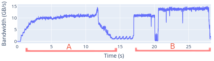
Figure 1. Difficulty of detecting I/O phases: Where does A finish? Is B one or two phases? How about A and B together?

Once the boundaries of the I/O phases are found, an average period could be calculated. However, using the average does not allow for differentiating I/O phases. For example, consider an application that has periodic large checkpoint writes that achieve high bandwidth, but also a single process that is often writing a few bytes to a small log file (thus with low bandwidth). Although the application is technically doing I/O while writing the log file, the periodicity of the checkpoint writes is what is the most interesting to contention-avoidance techniques such as I/O scheduling. If we simply see I/O activity as belonging to I/O phases and compute the average time between them, we may reach an estimate that does not reflect well the behavior of interest. Ideally, weighted average (e.g., weighted by the amount of transferred bytes) could be used to consider this, but other factors like slow I/O or sudden bursts make such an approach quickly reach its limitation.

We move away from detailed modeling approaches and averaging and focus on a simple metric: the I/O period. For that, we examine the I/O behavior in the frequency domain, instead of traditionally analyzing it in the time domain. In our approach, we treat I/O bandwidth over time as a signal, which we first discretize, then analyze using DFT. To exemplify our approach, consider Figure 2. We executed the IOR benchmarking tool (Benchmark, 2020) on the Lichtenberg cluster (see Section 4) with 2 segments, a block size of 10 MB, a transfer size of 2 bytes, and 8 iterations with the MPI-IO API in the collective mode. As illustrated in blue, the original signal has 8 phases that occur periodically. With our approach, we can easily identify the frequency of a signal which is 0.04 Hz corresponding to a period of 25 s. Even though there are I/O bursts present in the signal, our approach is capable of handling that while maintaining a low overhead as shown in Section 3.5.

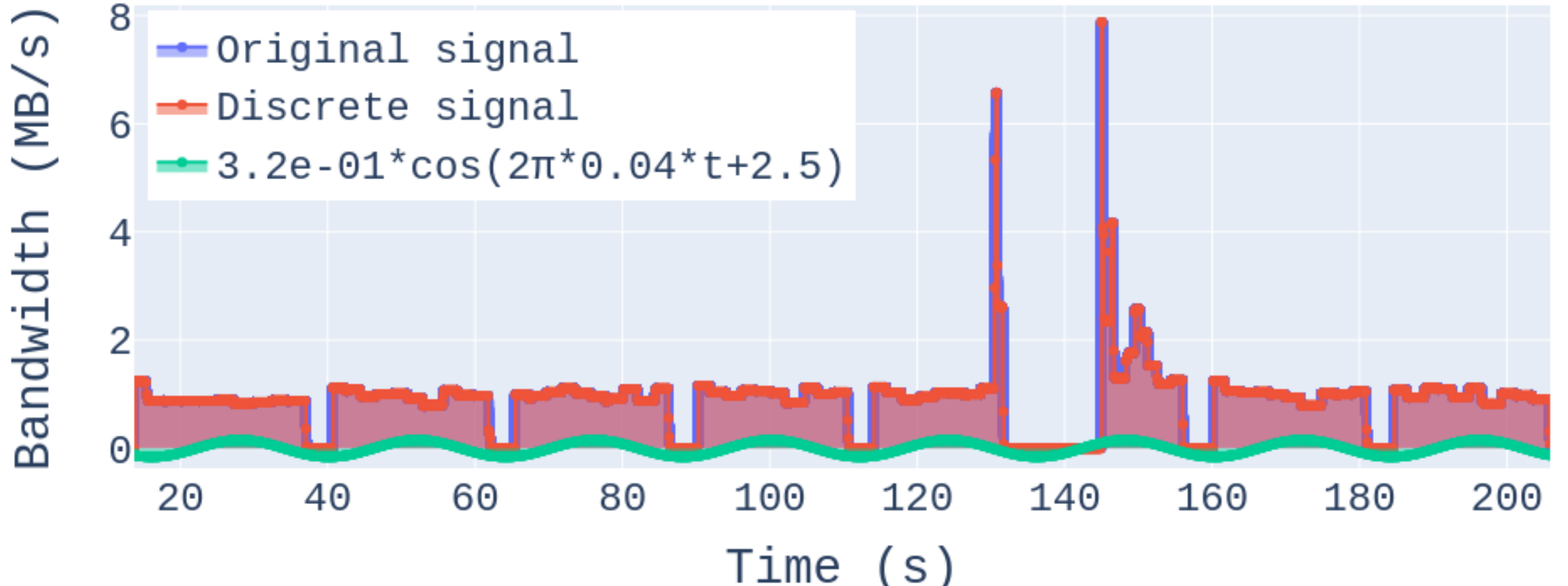
Figure 2. IOR with 1536 ranks. After discretization and DFT, the cosine wave that depicts the frequency of the I/O phases is found to be 0.04 Hz (i.e., a period of 25 s).

3. FTIO: finding the periodicity of I/O

In this section, we present our approach to predict the I/O phases of HPC applications using DFT. We call our methodology: Frequency techniques for I/O (FTIO). FTIO is implemented as a two-step approach: (1) a library at the application side intercepts the I/O calls and appends the collected data continuously to a file (Section 3.1), which (2) can be evaluated at any time (Section 3.2), on a cluster or a local machine, to determine the I/O periodicity. All the code is available at: hidden for double-blind. Besides briefly reviewing DFT, we examine the data collection, the key parameters of the approach, and the induced overhead. We also present additional metrics that try to measure how periodic the signal is and provide confidence metrics in the obtained results (Section 3.3).

3.1. Gathering the I/O information

As the first step of FTIO, the I/O information from the application needs to be collected. For this, we developed a tracing library (in C++) that intercepts specific MPI-IO calls to gather metrics such as start time, end time, and transferred bytes. We provide two methods for linking the library to the application, depending whether the information is used for offline (detection) or online (prediction) periodicity analysis. In the offline mode, the LD_PRELOAD mechanism is used, and upon MPI_Finalize, the collected data are written out to a single file that can be later analyzed. In the online mode, the library is included by the application and a single line is added to indicate when to flush the results out to a file (JSON Lines). This file can be evaluated at any moment using a Python script, for online prediction of the next phases based on the data collected up to this point. Note that, at the end of the run, the same file can be used for offline evaluation. Our library has a low overhead as the collected I/O data are at the rank level (individual requests), and their overlapping (i.e., bandwidth at the application level), is evaluated in the Python script (either entirely or for a given time window) with a linear complexity with the number of I/O requests.

In essence, what we need for the next step is the variation of the bandwidth over time. Since the analysis is at the application level, we merge the per-process collected information. Note that although we used our library in this paper, other tools, can easily provide this data, removing the need for our library. For example, for the detection approach, we support Recorder (Wang et al., 2020) traces. With our library, we aimed for a user-level implementation that could, however, be easily swapped with file system monitoring data, if available. Next, we describe how the collected information $x(t)$ (bandwidth over time) is used.

3.2. Predicting I/O periodicity using DFT

Fourier analysis has a wide range of applications including signal and image processing, analog signal design, physics (optics, astronomy, etc.), and many more. In essence, it decomposes a signal into its frequency components such that their sum allows for reconstructing the signal. While the term “Fourier transform” usually refers to the continuous one, which deals with continuous signals, the discrete Fourier transform (DFT) works with discrete samples of the signal in the time domain. Here, we use the latter.

DFT: DFT operates on discrete time values. Hence, we sample the continuous signal $x(t)$ with a sampling rate $T_{s}$ in a time window $\Delta t$, to obtain $N=\Delta t/T_{s}$ samples. That is:

(1) $$\{x_{n}=x(n\cdot T_{s})\quad|\quad n\in[0,N)\}$$

The sampling frequency, $f_{s}=1/T_{s}$, is the reciprocal of the sampling rate. The selection of $f_{s}$ is discussed in Section 3.4. DFT transforms the evenly spaced sequence (see Eq. 1) from the time domain into a sequence of the same length in the frequency domain:

(2) $$X_{k}=\sum_{n=0}^{N-1}x_{n}e^{\frac{-2\pi kn}{N}i}$$

for the frequency bins $k\in[0,N)$ corresponding to the frequencies:

(3) $$f_{k}=k\frac{f_{s}}{N}=\frac{k}{\Delta t}$$

DFT is evaluated for the fundamental frequency $\frac{f_{s}}{N}$ and its harmonics. In addition, the component at $f_{0}=0$ is referred to as the zero frequency component, DC value, or DC offset in signal analysis. Eq. 3 depicts that the complex values $X_{k}$ are $\frac{1}{\Delta t}$apart in terms of $f_{k}$. Hence, the larger the time window $\Delta t$, the closer the complex values $X_{k}$ are from each other on the frequency axis. However, increasing $\Delta t$ for a fixed sampling rate $T_{s}$, means more samples, which directly increases the complexity of the analysis.

As the sampled signal $x_{n}$ consists of purely real values, DFT is symmetric and only half of the frequencies are needed to reconstruct the signal with the inverse DFT (IDFT):

(4) $$x_{n} =\frac{1}{N}\left(X_{0}+\sum_{k=1}^{\frac{N}{2}}2|X_{k}|\cos{\left(\frac{2\pi kn}{N}+arg(X_{k})\right)}\right)$$

with the amplitude $|X_{k}|$ and the phase $arg(X_{k})$:

$$|X_{k}| =\sqrt{\operatorname{Re}(X_{k})^{2}+\operatorname{Im}(X_{k})^{2}}$$

$$arg(X_{k}) =atan2(\operatorname{Im}(X_{k}),\operatorname{Re}(X_{k}))$$

This reduces the calculation needed for the reconstruction of the signal as well as limits the constituting signals to cosine waves only, simplifying the interpretation of results. Consequently, when plotting the amplitude $X_{k}$ against the frequencies $f_{k}$, only half of the spectrum (single-sided spectrum) needs to be inspected. In this case, the amplitude of symmetric signals (around $\frac{N}{2}$) need to be multiplied by two as Eq. 4 shows (i.e., $2|X_{k}|$). Moreover, $X_{0}$ (DC offset) is expected to be among the highest components as the I/O data transferred is always a positive number of bytes, and the cosine waves obtained with DFT need to be shifted upwards. Moreover, dividing $X_{0}$ by $N$ results in the arithmetic average.

In this context, we can distinguish between three signals: the original, the discrete sampled, and the reconstructed with IDFT ones. All three are somewhat discrete, however, in contrast to the latter two, the points of the original signal (the I/O bandwidth over time) are not necessarily equally spaced by a fixed discretization step ($T_{s}$). Hence, in most cases, there is a variation between the original and the discrete signals. Moreover, in case all complex signals $X_{k}$ are used to reconstruct $x_{n}$, there is no difference between the discrete and the reconstructed signals, which is why we handle them identically. To compute DFT, we use the FFT (Fast Fourier Transform) algorithm, which has a complexity of $O(NlogN)$.

Results interpretation:

The result of DFT on the signal can then be visualized in the frequency domain, where the frequencies $f_{k}$ (or frequency bins $k$) are plotted against their corresponding amplitudes $|X_{k}|$.

Figure 3. Running example: IOR with 384 ranks.

As a running example, and to demonstrate how the period can be extracted from a signal, we run IOR on Lichtenberg cluster (described in Secion 4). We set up IOR with 384 ranks, 8 iterations, 2 segments, a transfer size of 2 MB, and a block size of 10 MB with the MPI-IO API in the parallel mode and our library preloaded. The temporal I/O behavior is shown in Figure 3.

Figure 4. Two-sided frequency spectrum from DFT for IOR with 384 ranks and a sampling frequency set to 100 Hz.

The result of DFT on this signal with $f_{s}=100$ Hz is shown in Figure 4, where the amplitudes $|X_{k}|$ are plotted against the frequencies $f_{k}$ for $k\in[0,N)$ (i.e., two-sided spectrum).

The amplitudes in the figure show the contribution of the frequencies to the signal: the higher the amplitude $|X_{k}|$, the more the frequency at $f_{k}$ contributes to the discretized signal $x_{n}$. This becomes especially interesting when one signal has a significantly higher amplitude than the others. If this is the case, the frequency of this signal (at $f_{k}$) delivers the periodicity of the I/O phases as it is the dominating one. As shown in Figure 4, 7605 (3803 for single-sided) frequencies contribute to the original signal. So the question is: How can we extract the dominating frequency, if there is any?

According to Section 3.2, it is enough to examine half the spectrum (i.e., $\frac{N}{2}$). Hence, we look into the single-sided spectrum which plots the amplitude of only half the data against the frequency. However, the amplitudes are adjusted: $2|X_{k}|$ for $1\leq k\leq\frac{N}{2}$ and $|X_{0}|$ for $k=0$.

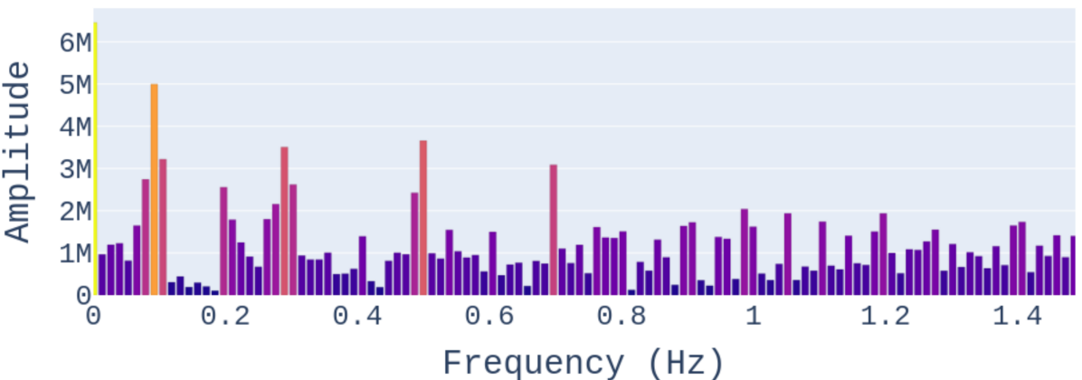
Figure 5. Single-sided spectrum from DFT on IOR with 384 ranks and a sampling frequency set to 100 Hz.

This is shown in Figure 5, for the running example from Figure 3. We added a color scale that shows the contribution of the amplitude to the aggregate amplitude over the $\frac{N}{2}$ frequencies. Higher values are closer to yellow while lower values are closer to dark purple. Since we set the sampling frequency $f_{s}=100$ Hz, and we are looking at the single-sided spectrum, one can expect to see frequencies up to 50 Hz. However, as the contribution of the frequencies up to 50 Hz is very low, we show only those up to 1.5 Hz. Moreover, the step between two consecutive frequencies is 0.013 Hz corresponding to $\frac{1}{\Delta t}$ ($\Delta t$ = 76.05 s). As shown in Figure 5, the contribution of the component at $f_{0}=0$ Hz is the highest. aligning with what has been stated at the beginning of this section.

Period extraction:

The most straightforward approach to extract the period of the I/O phases is to find the frequency with the maximum amplitude (i.e., the dominant frequency $f_{d}$), while excluding $f_{0}$. However, if there are multiple frequencies with amplitudes close to the maximum, they all have important contributions to the signal, i.e. the maximum-amplitude frequency does not properly represent it. Notably, that is the case for non-periodic signals. Hence, simply selecting the maximum would silently provide a result that is probably inaccurate. Therefore, the task narrows down to finding the frequencies with high amplitudes that are at the same time outliers. The number of such frequencies indicates the periodicity of the signal. One well-known approach for detecting outliers is the Z-score. It reveals how many standard deviations $\sigma$ an amplitude $|X_{k}|$ is from the mean $|\bar{X}|$ of the amplitudes:

(5) $$z_{k}=\frac{|X_{k}|-|\bar{X}|}{\sigma}$$

Thus for each frequency $f_{k}$, $k\in[1,\frac{N}{2}]$, a Z-score $z_{k}$ is found. Usually, a Z-score beyond 3 indicates an outlier. For the running example, we calculate the Z-score and found out that 80 out of the 3803 frequencies are candidates for outliers. That number is still too high to make reasonable conclusions concerning the periodicity. Hence, using a tolerance factor (which can be adjusted), we examine the largest Z-Scores of the outliers that lie 80% above the maximum. That is, the candidates $f_{k}$ that depict the period of the signal have:

(6) $${z_{k}\geq\max_{k\in[1,\frac{N}{2})}(z_{k})*80\%\geq 3}$$

If Eq. 6 is true, $f_{k}$ is a dominant frequency ($f_{d}$) candidate. We distinguish between three cases:

• High confidence: Only a single candidate frequency was found (i.e., Eq. 6 is true only once), which is $f_{d}$.

• Moderate confidence: Two candidate frequencies were found. The dominant frequency is the one with a higher amplitude.

• Low confidence: No dominant frequency was found (too many candidates, i.e., Eq. 6 was true at least three times).

Note that there is an exception. In case the candidates are multiples of two of each other, higher frequency values are ignored. The presence of these kinds of harmonics with decreasing high amplitudes in the frequency spectrum (like in Figure 5), is a direct indication that there are periodic I/O bursts (see Section 4).

Since a single frequency is expected for a perfectly periodic signal, the number of candidates provides confidence in the results. When three or more candidates are found, we have low confidence, as the signal might be non-periodic. Section 3.3 presents additional metrics that provide further confidence in the results.

For the running example,

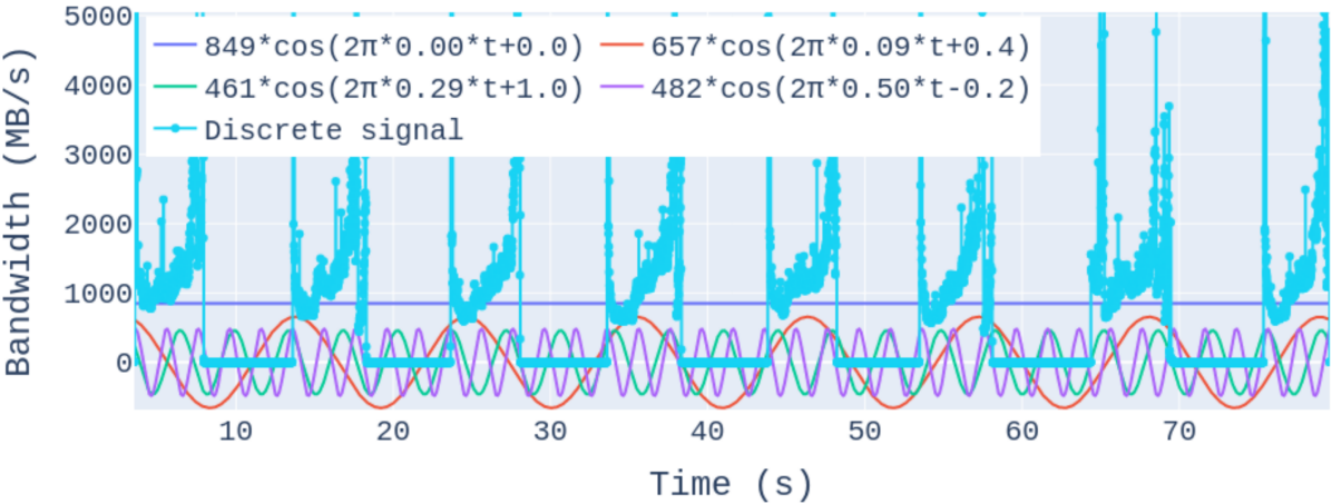
Figure 6. The cosine waves of the frequencies with the top four amplitudes (including $f_{0}$) plotted against time. The reconstructed signal, from all values, is also shown.

we plotted the top four signals with the largest amplitudes (including $f_{0}$) in Figure 6. The figure contains the discretized signal (zoomed) with $f_{s}=100$ Hz which is identical to the reconstructed signal (obtained from the IDFT). To show the contribution of a frequency, we extracted its corresponding component from Eq. 4 with ($t=nT_{s}$ and a zero-order hold) That is, the amplitudes of the cosine waves are $\frac{2X_{k}}{N}$ for $k\in[1,\frac{N}{2}$] and $\frac{X_{k}}{N}$ for $k=0$. Besides the offset at $f_{0}$, the frequency at $f_{7}=0.09$ Hz has the second-largest amplitude with a period of $\frac{1}{f_{7}}=10.86$ s. As mentioned earlier, 80 frequencies had a Z-Score larger than 3. By evaluating Eq. 6, only the Z-score of a single frequency at 0.09 Hz ($k=7$) satisfies the equation. Hence, $f_{d}=f_{7}$ and the the period of I/O phases is 10.86 s with high confidence, which is shown in Figure 7. Note that the first I/O operation starts at $t=3.5s$.

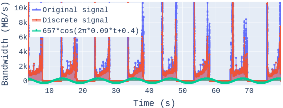
Figure 7. Result of our approach: The I/O behavior (blue) for the running example is periodic with a period of 10.86 s (i.e., $f_{7}=0.09$ Hz) as depicted by the signal in green.

Online prediction:

So far, we described the detection approach that is evaluate offline. For predicting the period online, the approach is similar, with the difference that DFT is periodically reevaluated once new I/O measurements are appended to the output file. For the running example, we added two lines to the ior.c file, one that includes the library, and one to flush the data out. Moreover, we modified the build commands to compile IOR with our library. During a different execution on Lichtenberg, we obtained 8 predictions. Unlike the previous (detection) example, the sampling frequency was set to 10 Hz and a bash script handled executing the Python script on the login node in distinct threads that return the periods. The first prediction didn’t find any dominant frequency, while the second one returned a period of $16.3$ s. The next six predictions returned: $12.9$, $11.8$, $11.5$, $9.5$, $11.2$, and $10.7$ s.

For online prediction, instead of considering the entire time window, it can be reduced. This is handled later in Section 3.4, which examines the parameters of DFT that can affect the analysis.

3.3. Additional characterization of I/O behavior

Our approach can find a dominant frequency for periodic I/O, that describes it well. However, non-periodic signals may lead to undetermined or simply wrong predictions. Therefore, metrics are required that provide a measure of how far from being periodic the signal is and, therefore, of the level of confidence in the obtained results. Although not formally defined, in this paper we talk about signals being “less” or “more periodic” to represent this idea. The number of candidate frequencies, discussed previously, is one of these metrics. In this section, we present two others.

The standard deviation of volume:

If we assume the application is periodic and we know its frequency, then in every period, roughly the same amount of data is transferred. For the I/O trace $\mathcal{T}$, let $V(\mathcal{T})$ be the amount of data accessed in it (i.e., “volume of I/O”). Given $f_{d}$ the frequency identified with DFT, we divide the trace into sub-traces $\{\mathcal{T}_{1},\cdots,\mathcal{T}_{Lf}\}$ each of length $\frac{1}{f_{d}}$ and amount of data V($\mathcal{T}_{i}$) for $i\leq Lf$. We compute $\sigma_{vol}$ as the standard deviation of $\frac{V(\mathcal{T}_{i})}{\max(V(\mathcal{T}_{i}))}$ (so it is between 0 and 1). The lower this value, the more similar the amounts of data accessed per period are, and thus the more periodic the signal. Note that an application could be periodic (in time) but not access the same amount of data per I/O phase, which will cause $\sigma_{vol}$ to be high. In that case, the $\sigma_{time}$ metric will quantify its periodicity “in time” only. Before we can define it, we first need to determine the time spent on interesting I/O.

Time spent on substantial I/O: An application could have frequent low-bandwidth I/O, for example by constantly writing a small log file, but periodic higher-bandwidth I/O phases. In this case, we consider the low-bandwidth activity as noise and the I/O phases as substantial (or interesting) I/O. On the other hand, for a signal composed only of the same low-bandwidth “noise”, we might desire to consider it not as noise but as the I/O behavior of that application. Therefore, we need a threshold of what is noise and what is interesting, identified for each application. A fixed per-system threshold could be enough for some utilizations of this method (such as I/O scheduling), but here we focus on the more challenging and generic case. For our trace $\mathcal{T}$ of length $L(\mathcal{T})$, we set our threshold as $V(\mathcal{T})/L(\mathcal{T})$, and let $\mathcal{S}$ be the subset of the time-units of the trace where the volume of I/O per time-unit is greater than this threshold. Then, having filtered out the noise, we can compute the time ratio spent doing substantial I/O: $R_{IO}=L(\mathcal{S})/L(\mathcal{T})$, with $R_{IO}\in[0,1]$. We can also identify the bandwidth characterizing the substantial I/O of the whole trace: $B_{IO}=V(\mathcal{S})/L(\mathcal{S})$. This is illustrated in Figure 8.

Figure 8. A red line marks the $V(\mathcal{T})/L(\mathcal{T})$ threshold in the trace from Figure 1. Here $R_{IO}=0.68$ and $B_{IO}=\approx 11$ GB/s.

The standard deviation of time:

Similarly to $\mathcal{S}$, we let $\mathcal{S}_{i}$ be the subset of $\mathcal{T}_{i}$ where the volume of I/O per time-unit is greater than $V(\mathcal{T})/L(\mathcal{T})$. Then The standard deviation of time is:

(7) $$\sigma_{time}=\sqrt{\frac{1}{L\cdot f}\sum_{i=1}^{L\cdot f}\left(\frac{L(\mathcal{S}_{i})}{L(\mathcal{T}_{i})}-R_{IO}\right)^{2}}$$

In other words, $\sigma_{time}$ is the standard deviation of the proportion of time spent on I/O inside each period. The intuition is that, if the signal is periodic, and the application spends, e.g., $60\%$ of its time on I/O ($R_{IO}=0.6$), then each of its I/O phases lasts approximately $60\%$ of a period. Therefore, the lower the $\sigma_{time}$, the more periodic the signal is expected to be. Values close to zero for both $\sigma_{time}$ and $\sigma_{vol}$ indicate a signal that is periodic and therefore a high confidence in the period obtained with FTIO. On the other hand, a high $\sigma_{vol}$ with a low $\sigma_{time}$ indicates the application is probably periodic but does not access similar amounts of data per I/O phase.

Amount of data per period:

The amount of data transferred per period is calculated as $\frac{V(\mathcal{S})}{L(\mathcal{T})\times f_{d}}$, and the lower $\sigma_{vol}$, the better this value works as a prediction for a future I/O phase.

Periodicity score:

Finally, since both $\sigma_{vol}$ and $\sigma_{time}$ are in $[0,0.5]$, we can provide a periodicity score (between $0$ and $1$) for the signal according to the FTIO-provided period as $1-$$\sigma_{vol}$ $-$$\sigma_{time}$.

3.4. Parameter Selection

According to Section 3.2, three parameters can affect the analysis: the time window $\Delta t$, the sampling rate $T_{s}$ (i.e., sampling frequency $f_{s}$), and the number of samples $N$. Note that two of these parameters can be selected, while the third is obtained from $N=\frac{\Delta t}{T_{s}}$.

The sampling frequency $f_{s}$ specifies at which granularity the data is captured. As our approach captures the time spent on each I/O request, we can find the smallest change in bandwidth over time. However, this is often not needed, as we are usually not interested in high-frequency behavior. For the running example, $f_{s}$ set to 10 Hz would have yielded the same results. However, a too-low sampling frequency could result in aliasing and thus mislead the analysis. This is illustrated in Figure 9, which shows the results of FTIO on miniIO (miniIO Benchmark, 2022) executed with 144 ranks on the Lichtenberg cluster. The unstruct mini-app was used, which produces unstructured grids with 1000 points per task. Here, we set $f_{s}$ to 100 Hz, which is still not enough, as shown in the figure, as the discrete signal does not match the original one at all. For this sampling, our approach indicated that the signal is not periodic, as there are too many dominant frequencies. But even if the approach had found a single period, the result cannot be trusted, as the abstraction error (the volume difference between the two shown signals) is just too large.

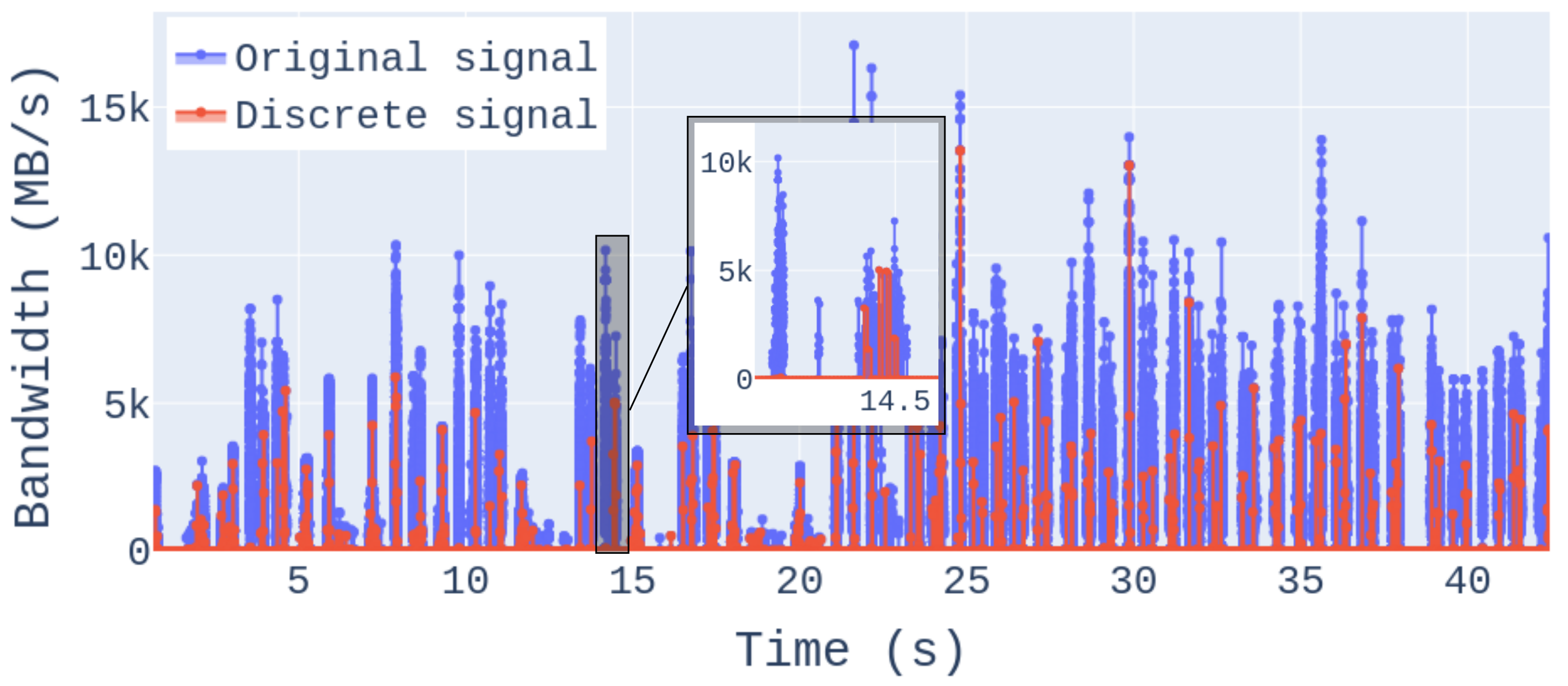
Figure 9. miniIO with 144 ranks on the Lichtenberg cluster. No prediction was generated for this example.

With a constant sampling rate $T_{s}$, increasing $\Delta t$ increases the number of samples $N=\frac{\Delta t}{T_{s}}$, which increases the detection/prediction time. In all of our experiments, this time was negligible. Moreover, it does not represent overhead to applications, since the analysis is not done on the nodes where they run. The only overhead comes from the tracing library and is analyzed in Section 3.5. For online evaluation, since the I/O behavior of an application can change, it makes sense to discard the old data at some point and consider a shorter time window. Hence, to adapt to changing I/O behavior, our algorithm is that after finding three times a dominant frequency, the time window for evaluation is reduced to three times the last found period. Alternatively, one could specify a fixed length for the time window.

3.5. Overhead of the tracing library

The tracing library can be used for offline detection or online prediction. From those, we examine the online approach as it has a higher overhead, since it sends information to the file more often (see Section 3.1). To measure it, we executed IOR with the same settings as in Section 3.2, on the Lichtenberg cluster (see Section 4) with different numbers of processes (all multiples of 96 as this is the number of cores in a typical node). Figure 10 shows the overhead of the tracing library, with the top part showing aggregated time, while the bottom plot shows the time from the MPI rank 0 perspective only. The numbers of ranks on the x-axis are in log scale and the sum of the application time (App) and overhead is the total time.

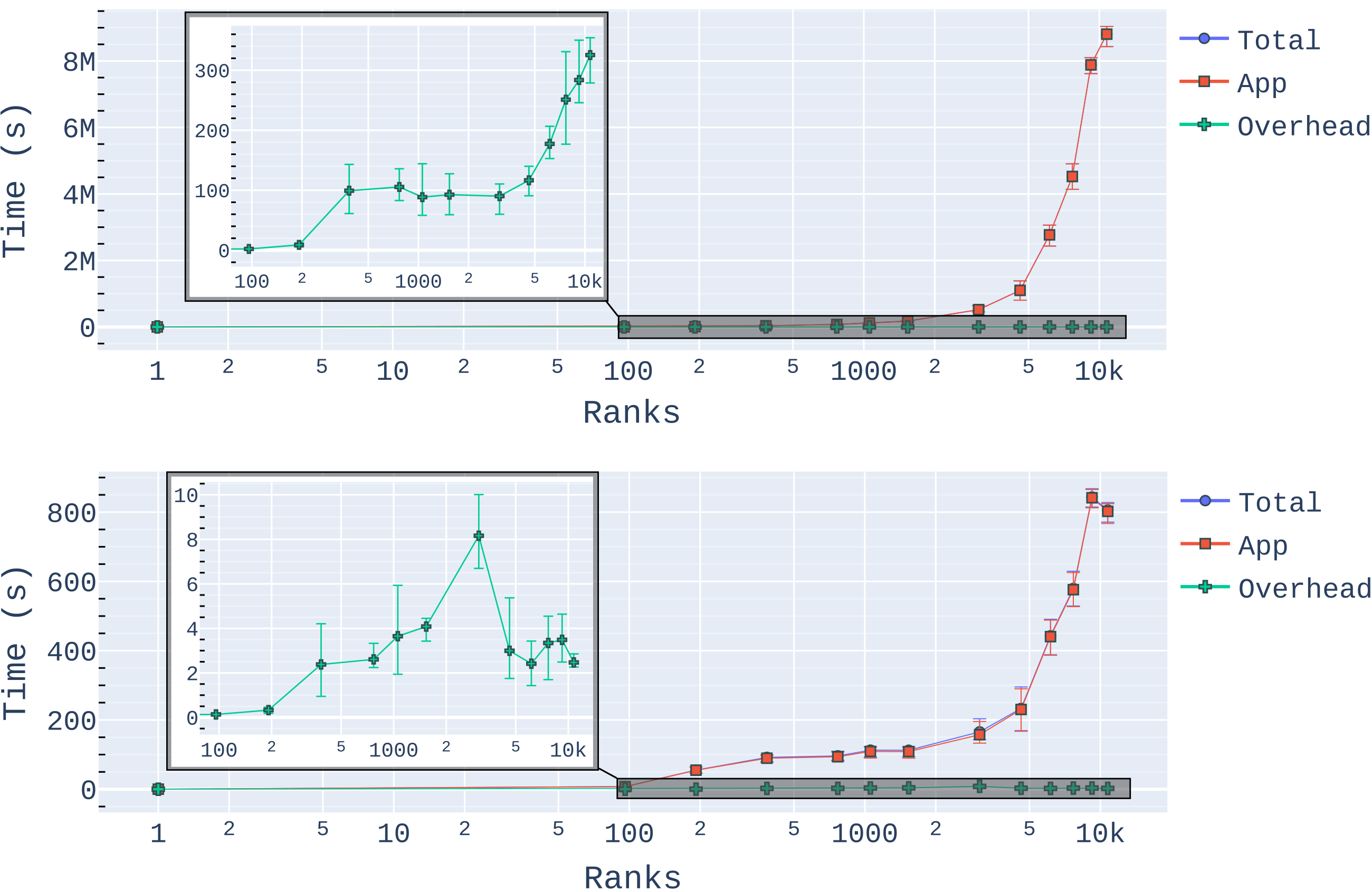
Figure 10. Overhead of our approach across different rank configurations. The top shows the aggregated time across the ranks, while the bottom shows the time of rank 0 only.

As observed, for capturing and logging the I/O data, our tracing library has a low overhead: a maximum of 0.6% for the aggregated overhead and 6.9% for the overhead for rank 0 only. The data gathering from the different ranks is the major source of overhead. For comparison, in the same configurations, the overhead obtained by the offline approach increased nearly linearly from 0.78 s at 96 nodes to 50.9 s at 4608 ranks in the aggregated overhead time and from 0.065 s to 3.84 s for the overhead for rank 0 only.

The execution time of the analysis is of minor importance, as mentioned, and depends on the length of the time window. For the use cases is Section 4, the longest analyzes took: 2.4 s for LAMMPS and 15.8 s for IOR for their entire time windows, and 8.3 s for HACC-IO with an adapted time window. As a prediction may not be done by the time new data becomes available, we used a bash script to launch prediction threads. It is important to notice that our approach could be used with other data collection strategies, such as integrated into a monitoring framework, which would have different implications. For example, if implemented in a profiling tool such as Darshan, it could leverage the data collection and aggregation architecture already in place.

4. Experimental runs

To evaluate our method, in this Section we: (i) discuss scalability using the IOR experiment from Section 3.2 but with more processes; (ii) use a mini-app (HACC-IO) with high I/O bandwidth to highlight the detection and prediction capabilities of FTIO, and (iii) analyze a real application (LAMMPS) with low I/O bandwidth. The use cases (ii) and (iii) also differ in the amount of accessed data, number, and frequency of I/O activity (all heavier in HACC-IO than in LAMMPS). All experiments in this section were performed on the Lichtenberg cluster, where the typical node has 96 cores and the access mode is user-exclusive. The shared file system (IBM Spectrum Scale) has peak performance of 106 GB/s for writes and 120 GB/s for reads.

Scalability:

Our first use case illustrates the applicability of our approach at a large scale. For that, we executed the IOR benchmark with 9216 ranks (see Section 3.2 for the full settings). As we can see in Figure 11, FTIO detected the period of the signal which is 111.67 s (i.e., 0.01 Hz). Note that, as mentioned in Section 3.2, the harmonic at 0.02 Hz is ignored, and its presence as a candidate for the dominant frequency is an indication of the presence of periodic I/ O bursts in the signal.

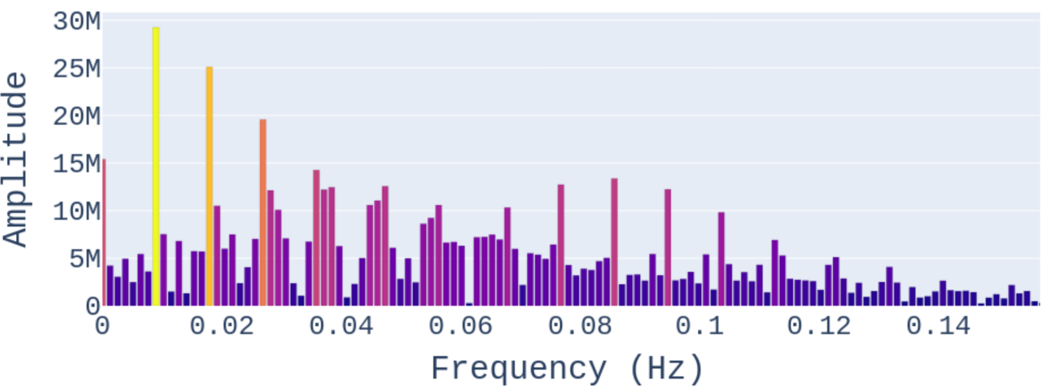
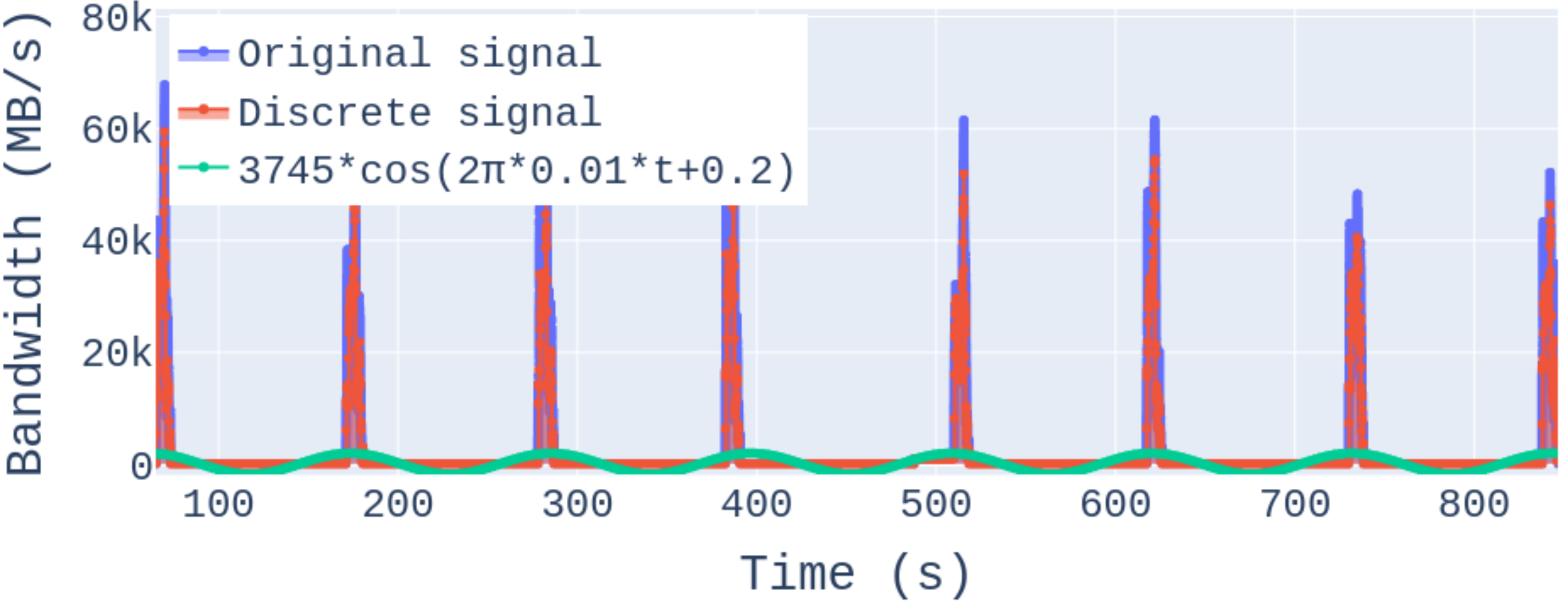
Figure 11. FTIO results on IOR with 9216 ranks.

Detection and prediction with high I/O bandwidth:

In the next experiment, we study HACC-IO (LLNL, 2020), which mimics an I/O phase of HACC (Hybrid/Hardware Accelerated Cosmology Code) (Habib et al., 2012). HACC-IO has four steps: compute, write, read and verify. We added a loop around these steps to execute them several times. Moreover, at the end of each loop iteration, we added a single line to flush the collected data out to the trace file. On a login node, we deployed the script that performs the prediction every time new data is available (i.e., the trace file is appended). We executed this example with 3072 ranks on the Lichtenberg cluster.

1) Offline evaluation: We first look into the output of the offline evaluation performed over the whole trace after the end of the execution. The single-sided spectrum is presented in Figure 12.

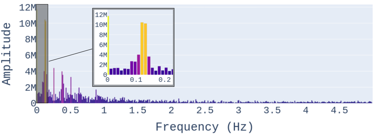
Figure 12. Single-sided spectrum from DFT on HACC-IO with 3072 ranks and a sampling frequency of 25 Hz.

Two candidates for the dominant frequencies were found: 0.1206 Hz and 0.1326 Hz. The former has the highest amplitude, hence FTIO detects a period of $8.29$s with moderate confidence (see Section 3.2).

Note that the application is by design periodic. However, if we study qualitatively the execution in Figure 13, we can see that, because of a period of slow I/O, the first I/O phase was significantly longer than the others: it lasts from $4.1$ to $15.3$ s. That makes this signal less periodic and explains our moderate confidence. Indeed, the average time between the start of consecutive I/O phases is $8.7$, but $7.7$ without the first I/O phase. Figure 13 presents the top three signals present in the temporal I/O behavior. As shown, the I/O phases align more with the 0.120 Hz signal (red) at the start, and with the 0.132 Hz signal (green) near the end.

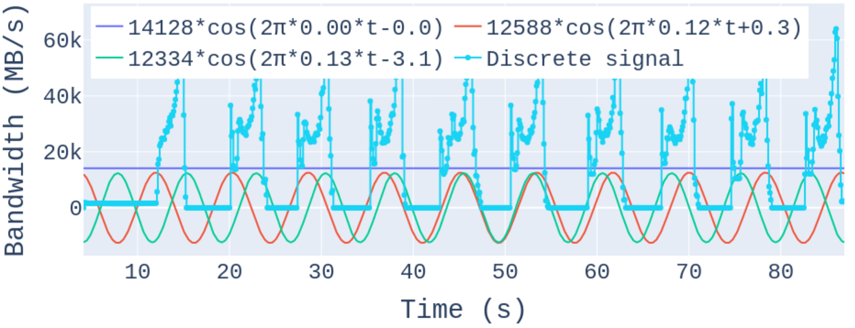
Figure 13. DC Offset and highest-amplitude frequencies found in the temporal behavior of HACC-IO with 3072 ranks.

As the two candidates for the dominant frequency have very close amplitudes and are consecutive, one approach could be to merge them by taking the sum of their cosine waves. This is shown in Figure 14, and would provide a more accurate representation of the application’s temporal I/O behavior. However, in this paper, we focus on representing that behavior by a single period, which is concise and can easily be used as input for techniques such as I/O scheduling. Contrary, a more detailed application profile could include several dominant frequencies and their amplitudes, allowing for reconstructing the signal. We plan on exploring such profiles as future work (see Section 7).

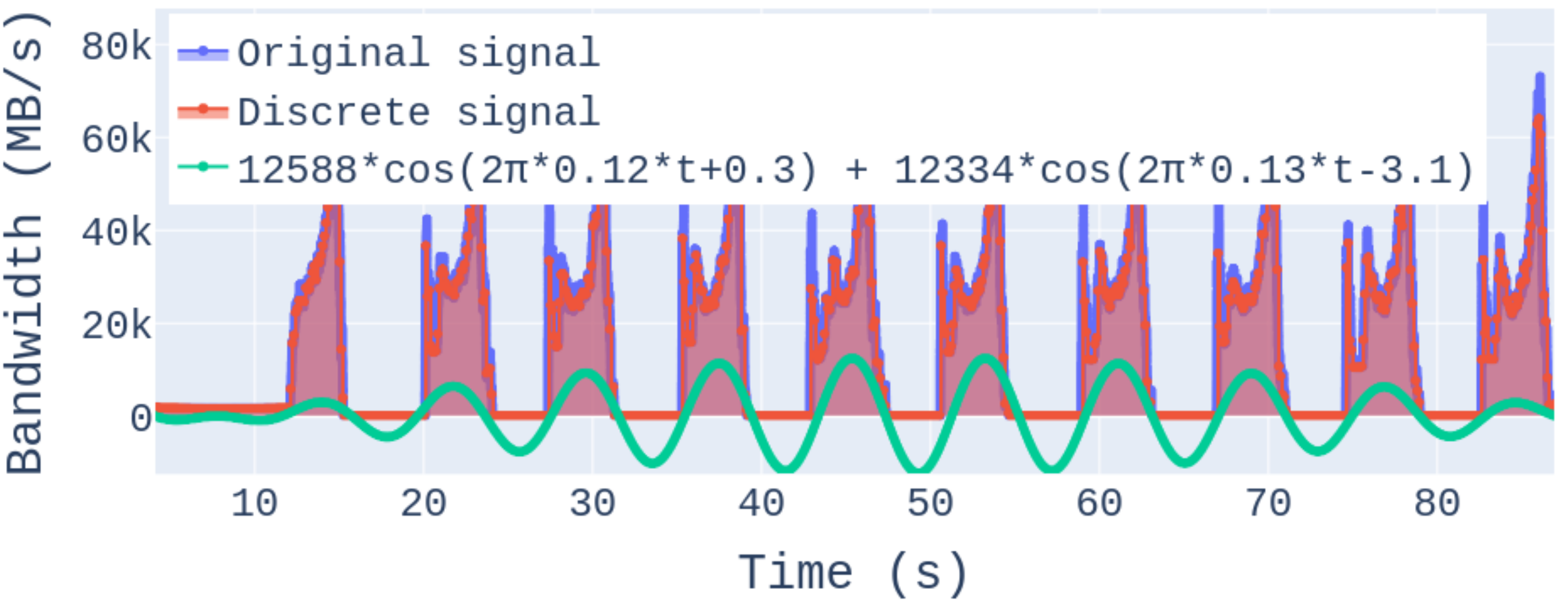
Figure 14. HACC-IO with 3072 ranks.

2) Online Prediction As discussed in Section 3.4, the time window for FTIO predictions can be adapted according to the found frequency. For the ten I/O phases which started on average every 8.7s, the average obtained prediction is 8.66s. All predictions are shown visually in LABEL:fig:hacc-online. To read it: predictions are done at the end of each I/O phase (dashed vertical lines), when data becomes available. At the end of the $3^{th}$ prediction, a dominant frequency was identified for the third time. As the $4^{th}$ prediction had already started, that information was made available for the $5^{th}$ prediction. Hence for the next evaluation, we only kept the data between time 47.4s (time of the $5^{th}$ prediction) and $47.4-3\times 8.1=23.1s$ for the evaluation (this is represented visually in bold). The same thing happened to the $8^{\text{th}}$ prediction ($71.1-3\times 8=47.3$s).

(a)

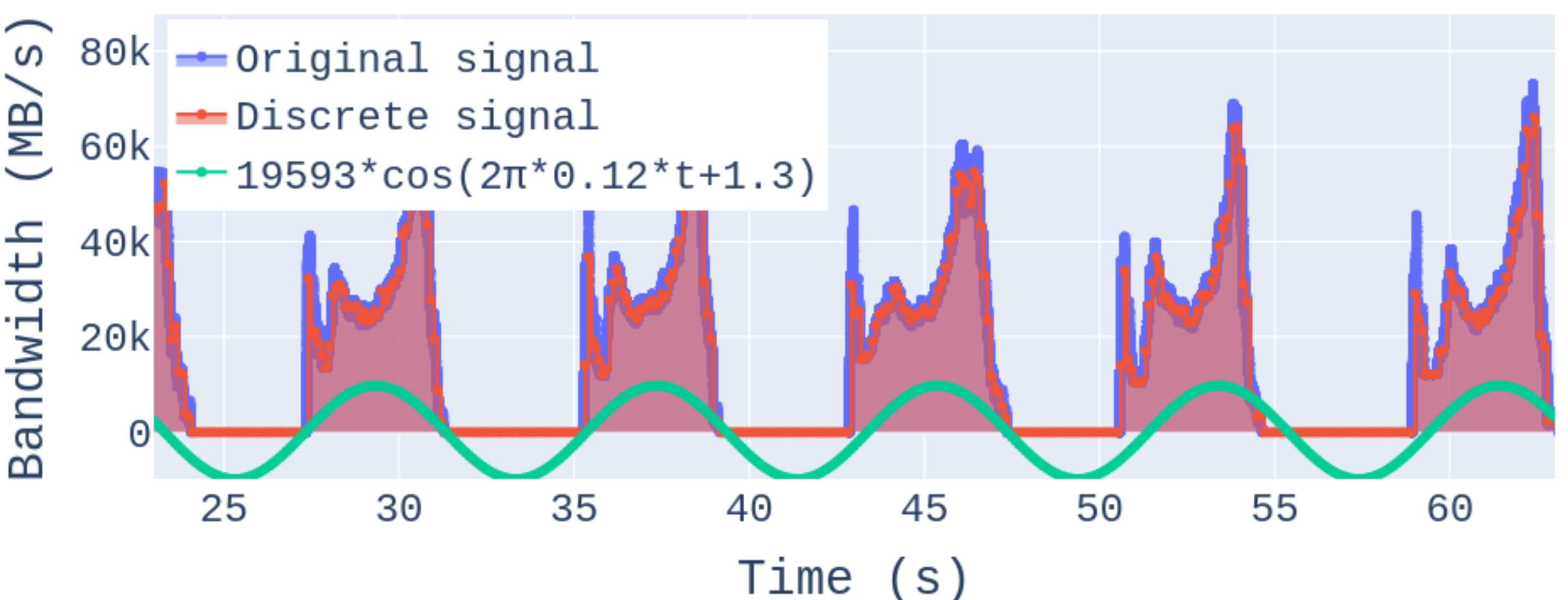
(b)

Figure 15. Online prediction during the execution of HACC-IO with 3072 ranks.

Real application with low I/O bandwidth:

Finally, we demonstrate our approach with LAMMPS (Thompson et al., 2022) on 3072 ranks. We choose the 2-d LJ flow simulation with 300 runs and dump all atoms every 20 runs. Using FTIO with $f_{s}=10$ Hz in the detection mode, the result was obtained in 2.4 s. The single-sided frequency spectrum is shown in Figure 16.

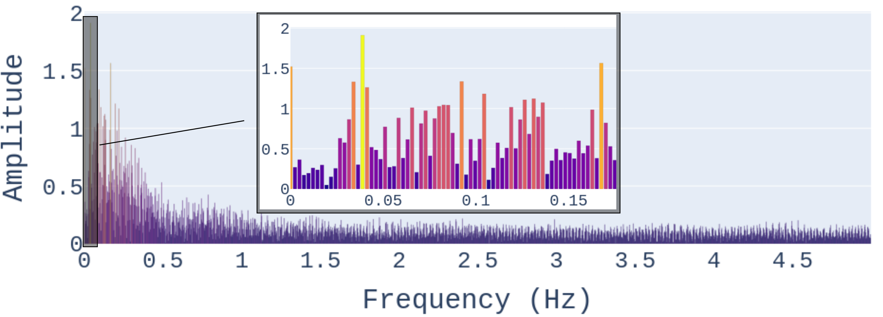
Figure 16. Single-sided spectrum from DFT on LAMMPS with 3072 ranks.

As illustrated, the approach found two dominant frequency candidates, one at 0.039 Hz (25.73 s) and one 0.16 Hz (5.9 s), which gives us a moderate level of confidence in the obtained results. Since the signal at 0.039 Hz has a higher amplitude, FTIO detects $25.73$ s as the period as shown in Figure 17. For comparison, the real mean period for this execution was 27.38 s.

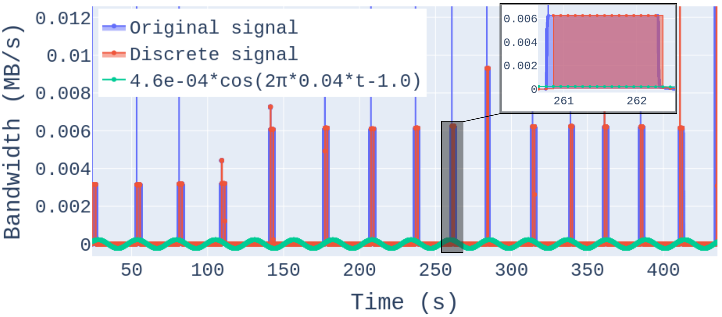
Figure 17. Result of FTIO on LAMMPS with 3072 ranks.

The figure also shows low I/O performance due to the writing method. The weak confidence is justified, as one can see that the dominant frequency does not apply to all phases (e.g., at 143 s). Still, it provides an adequate and concise representation of the temporal I/O behavior of the application, which is what we wanted. Note that, by adapting the time window for online prediction, the obtained results will be better, as was observed earlier for HACC-IO.

Summary of the results:

The experiments in this Section have demonstrated the use of FTIO with large-scale applications, for both offline detection and online prediction, with good results. For HACC-IO and LAMMPS, variability (in I/O performance for HACC-IO and in time between I/O phases for LAMMPS) caused the signal to be less periodic, resulting in a moderate confidence in the obtained results. The observation from HACC-IO indicates that, in these situations, the online prediction approach can yield the best results by adapting the time window.

5. The limits of FTIO

In Section 4, we showed our FTIO provides good results by using large-scale applications on a production system. In this Section, we explore its limitations by crafting challenging traces.

Methodology:

To allow for an extensive evaluation, we have created “semi-synthetic” traces: first, we traced IOR runs that represent a single I/O phase. Then we generated application traces by combining I/O phases with a given amount of “idle” (no I/O) time between them. IOR was executed ($100$ times) on the PlaFRIM cluster: 32 per-process $3.5$ GB files are written in $1$ MB contiguous requests using eight processes per node. The average I/O phase duration was $11$ s ($\approx 10$ GB/s), with all inside $[10.4,14.7]$ s.

We consider an application to be a sequence of $J$ non-overlapping iterations. Each iteration $j\leq$ $J$ is composed of a compute phase of length $t_{cpu}^{(j)}$ followed by an I/O phase where each of the $P$ processes write an amount of data $v$ to the file system. The trace is created by selecting $J$ and P, and then, for each $j\leq$$J$, by:

1. drawing $t_{cpu}^{(j)}$ from a normal distribution $\mathcal{N}(\mu,\sigma)$ truncated so only positive values are selected;

2. randomly picking one of the I/O phase traces, which consists of $P$ per-process traces;

3. for each process $k\in[1,P]$, adding a time $\delta_{k}$ at the beginning of its trace (without I/O). $\delta_{k}$ is drawn from an exponential distribution of average $\phi$. Process $0$ has $\delta_{0}=0$ to keep the boundaries of the I/O phase.

$\delta$ allows us to represent both desynchronization between processes and I/O variability, because the length of the I/O phases will depend on $\delta$. Finally, for experiments with noise, we generated $200$ traces from IOR on a single process in two configurations: low noise of $\approx 500$ MB/s and high noise of $\approx 1$ GB/s. The noise traces have 10 periods of approximately $2.2$ s each. Noise is emulated by randomly selecting a sequence of noise traces and adding them to the application trace. For all experiments in this Section, we used $f_{s}=1$ Hz, $P=32$ (the number of processes used for IOR), and $J$$=20$ (to be able to induce enough variability in each trace). Figure 18 illustrates traces created with this approach.

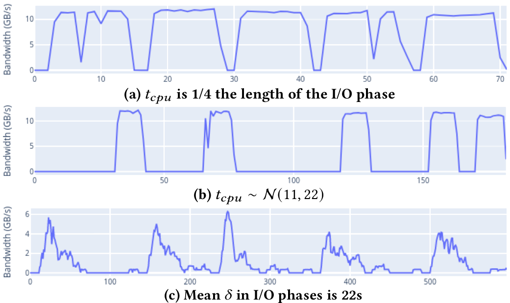
Figure 18. Examples of “semi-synthetic” application traces.

We generate $100$ traces per parameter combination. For each one, we compute $\lambda_{avg}$ the average iteration length and $\lambda_{FTIO}$ the period obtained with our approach. Finally, we calculate the detection error as $|\lambda_{FTIO}-\lambda_{avg}|/\lambda_{avg}$. Note that the $\lambda_{avg}$ can only be computed using information from the trace generation, notably the boundaries of I/O phases, that are not typically available. Reaching a low error means FTIO provides a value that is close to the average period,

Results:

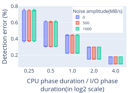
(a) … time between I/O phases (relative to their length) and noise.

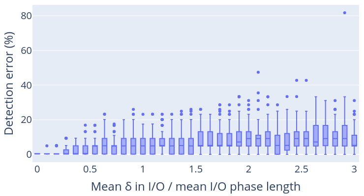
(b) … mean $\delta$ added to processes’ I/O phases.

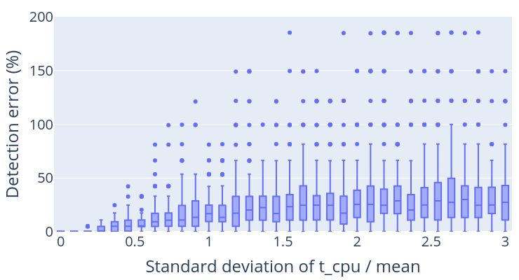
(c) … variability of time between I/O phases.

Figure 19. Detection error as a function of the …

First, we study the impact of a length difference between CPU and I/O phases, e.g. as seen in Figures 11 and 17. For this, we used traces with $\delta$ $=0$ and vary $t_{cpu}$ (while keeping its standard deviation to 0). Results are presented in Figure 19(a) and show that the disparity in phase length is not a problem. They also seem to indicate that when the time between I/O phases is longer, our approach leads to better results. However, that might be an artifact of the fixed sampling rate. Still, all the errors are below $1\%$. These results also indicate FTIO is somewhat robust to noise.

We now cover two challenging scenarios at once: first, when the processes performing the I/O phase are not synchronized (there is no implicit or explicit barrier) and thus start and end their operations at different times; and second, I/O performance variability, with some I/O phases of the application taking longer than others, which is usual the case when accessing a shared PFS. For that, we set $t_{cpu}=11$ s and increased $\phi$ (the average $\delta$). The results are presented in Figure 19(b). When the mean $\delta$ becomes larger than the original I/O phase length, there are often periods without I/O activity inside the I/O phases, which makes the detection more difficult. We can see that in extreme cases, the error can go up to $80\%$, but it is in general below $20\%$.

Finally, we study the case where the time between I/O phases varies during the execution, as in Figures 11 and 17. We control that by drawing $t_{cpu}$ from $\mathcal{N}(\mu,\sigma)$ with $\mu=11$ s and increasing $\sigma$ (the standard deviation). For this experiment, we use $\delta$ $=0$ and there is no noise. It is important to notice that the traces still present variability, due to the use of real I/O traces for the phases. In Figure 19(c), we can see results vary in quality as the signal becomes less periodic. This figure was zoomed-in to allow the visualization of the box plots. $213$ outliers with error of more than $75\%$ are not shown (out of $3400$ traces). They are: $0.7\%$ of the traces with $0.5\mu\leq\sigma<\mu$, $6.7\%$ with $\mu\leq\sigma<2\mu$, and $11\%$ of the traces with $\sigma\geq 2\mu$. Starting from $\sigma/\mu=0.3$, at least $25\%$ of the traces obtained low or moderate confidence, and that number goes to $50\%$ when $\sigma/\mu=0.55$. For all cases, the calculated $R_{IO}$ is wrong by less than $10\%$.

Figure 20 presents the metrics $\sigma_{vol}$ (left) and $\sigma_{time}$ (right) for this experiment. As shown, both increase as the variability increases (i.e. the signal becomes “less periodic”). Their variability for each point from the x-axis matches the variability observed in the error shown in Figure 19(c). The median confidence, calculated as $1-$$\sigma_{vol}$ $-$$\sigma_{time}$, is over $90\%$ for $\sigma=0$, then drops below $75\%$ for $\sigma/\mu=0.4$, and below $50\%$ for $\sigma/\mu=1.3$. These results show that, for the situations where the detection error could be higher, the metrics indicate how far from being periodic the signal is, and thus how much we should trust the detections. Hence, when designing a technique (e.g., I/O scheduling) that uses the output from FTIO, one can study the robustness of their technique according to the values of $\sigma_{vol}$ and $\sigma_{time}$ to decide on thresholds for these metrics, since some approaches will tolerate higher detection errors than others.

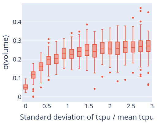
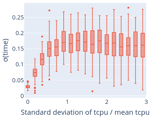
Figure 20. Metrics from the experiments in Figure 19(c).

6. Related Work

Because I/O performance depends on many parameters (Pottier et al., 2020; Wang et al., 2019; Chowdhury et al., 2019; Yang et al., 2019; Isakov et al., 2020), profiling tools such as Darshan (Carns et al., 2009; Snyder et al., 2016) and other more holistic approaches (Lockwood et al., 2017; Xu et al., 2016) can be used by an expert to obtain insights about application I/O behavior and improve it. However, these large profiles are not easily automatically exploitable at run time by optimization techniques, which must focus on simpler metrics. For example, in the context of cache management and I/O prefetching, it is useful to predict the future I/O requests (Dryden et al., 2021). That has been done using neural networks (Tseng et al., 2019), ARIMA time series analysis (Tran and Reed, 2004), pattern matching (Tang et al., 2014), context-free grammars (Dorier et al., 2016), etc. Although our FTIO could be used to predict future accesses, it is fundamentally different from these because we focus on I/O phases, not I/O requests. Working at this higher level brings the challenge of not knowing when I/O phases start and end (because they are a logical grouping of I/O requests, not explicit events).

More general characterization efforts usually focus on aspects such as spatiality and request size (Lu et al., 2014; Davis et al., 2010), for example using information from MPI-IO (Liu et al., 2013; Ge et al., 2012; Song et al., 2011) or ML-based methods (Bez et al., 2019). In contrast, we focus on the temporal behavior (and more specifically on the periodicity), hence our FTIO is complementary to these. Boito et al. (Boito et al., 2022) have shown that the periodicity information is sufficient to allow for good contention-avoidance techniques (e.g. in scheduling I/O accesses).

In the field of performance analysis, Casas et al. (Casas et al., 2010) proposed to construct signals of metrics (e.g. number of active processes, amount of communicated data, etc), and then to apply discrete wavelet transform to keep the highest-frequency portions, and auto-correlation to find the frequency of the application’s phases. We were inspired by the use of signal processing techniques, but our approach is different because they aim at removing the effects of external noise to detect the phases that best represent the application, while we searched for a lightweight approach to concisely represent the periodicity of the I/O behavior. Yang et al. (Yang et al., 2022) proposed a metric to quantify the burstiness of I/O and apply it to traces from a production machine. They found that most traces presented a very high degree of burstiness, however their metric is a measure of “uneveness”, not of periodicity, which is our focus.

Qiao et al (Qiao et al., 2020) used DFT on a signal of I/O performance per call of a write routine. They used it to search for the period of interfering applications (and using that to predict future interference). By Nyquist, they can only find frequencies lower than half the frequency of their write routine. We argue for a scenario where this information can be easily obtained for all applications and shared so smart decisions can be made throughout the system.

7. Conclusion and Final Remarks

In this paper, we presented the FTIO approach to characterize and predict the temporal I/O behavior of an application with a simple metric: its period, obtained using DFT. Besides its low overhead, we showed its applicability to real examples as well as its behavior in extreme cases, and presented several metrics to evaluate the results.

We focused on application-level characterization and studied a single signal (total bandwidth change over time) composed of I/O accesses coming from different processes. Nonetheless, there are situations where one could be interested in the processes’ behaviors, for example, for cache management (e.g. burst buffers). Our approach would work the same when applied at different levels. Furthermore, although we focused on I/O in this paper, the technique is applicable on other use cases — by changing the input data — such as finding the periodicity of scheduling points.

Our discussion on the selection of the sampling frequency (see Section 3.4) assumes we are interested in any frequency the application presents. In some techniques, such as I/O scheduling, we may not be interested in high frequencies (I/O phases that happen too fast and too often) because there is no time to do something about them. In that case, the sampling frequency could be selected as fast enough to capture the relevant frequencies.

In other contexts, such as the exact design of a profile, we may be interested in different information: not only in the period of a signal but also in for how long this period is valid. However, DFT has a high-frequency resolution but no time resolution (i.e, we don’t know when a frequency occurred). In this case, our approach may show its limits and the wavelet transformation (Graps, 1995) may be more appropriate. It would come, however, at a price of a larger overhead and lower accuracy in the frequency domain. Another important cost of wavelet transform compared to FTIO is the interpretability of the result. To see this, we performed some preliminary evaluation on the IOR example from Section 4 with 9216 ranks. The result for a decomposition level of ten of the continuous wavelet on the signal is shown in Figure 21. The color scale shows how present a particular frequency is at a given time in the signal (i.e., the amplitude of the wavelet coefficients).

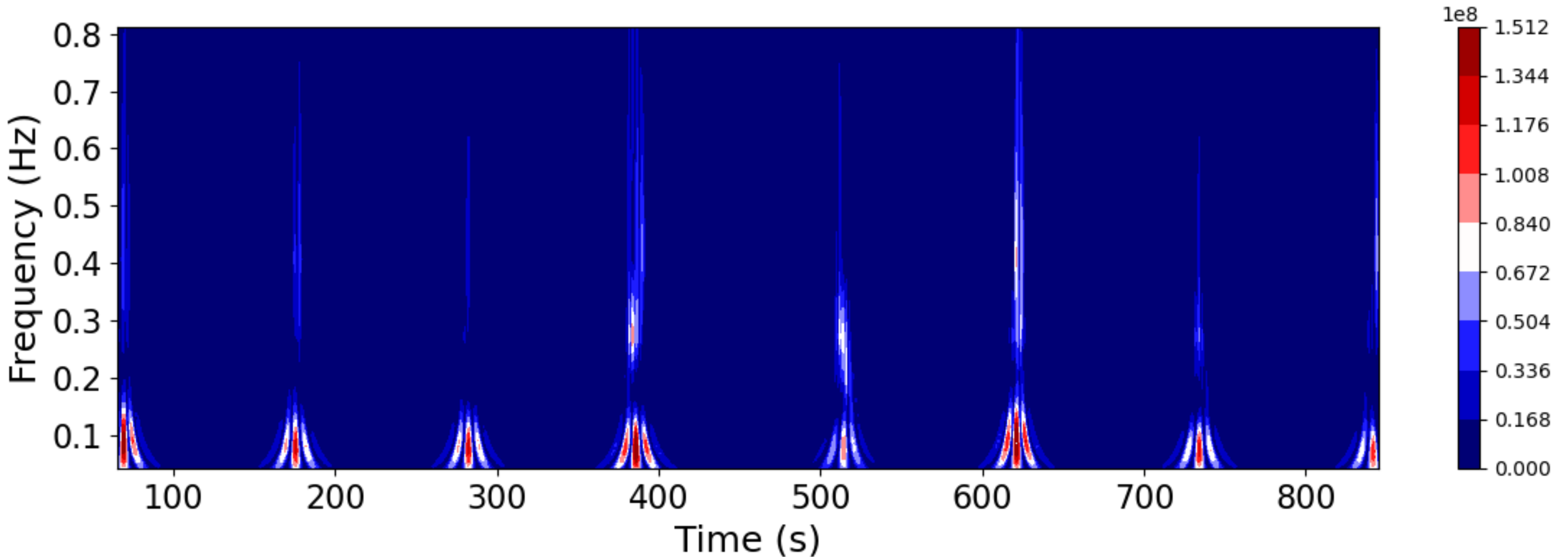
Figure 21. Continous wavelet transformation on IOR with 9216 ranks with a decomposition level of ten.

We can clearly see the I/O phases as the red regions in Figure 21, but it is harder to extract a frequency. Hence, unlike DFT, the evaluation of the wavelet transformation needs more sophisticated methods. This is also a reason why we left it out for future work. Finally, we believe that those two approaches (DFT and Wavelet Transform) are complementary, and the best choice depends on the finality of the analysis.

References

- (1)
- Aupy et al. (2018) Guillaume Aupy, Olivier Beaumont, and Lionel Eyraud-Dubois. 2018. What size should your buffers to disks be?. In 2018 IEEE International Parallel and Distributed Processing Symposium (IPDPS). IEEE, 660–669.
- Benchmark (2020) IOR Benchmark. 2020. Version 3.3.0. https://github.com/hpc/ior.
- Benoit et al. (2023) Anne Benoit, Thomas Herault, Lucas Perotin, Yves Robert, and Frédéric Vivien. 2023. Revisiting I/O bandwidth-sharing strategies for HPC applications. Technical Report RR-9502. INRIA. 56 pages. https://hal.inria.fr/hal-04038011
- Bez et al. (2019) Jean Bez, Francieli Boito, Ramon Nou, Alberto Miranda, Toni Cortes, and Philippe O.A. Navaux. 2019. Detecting I/O Access Patterns of HPC Workloads at Runtime. In SBAC-PAD 2019 - International Symposium on Computer Architecture and High Performance Computing. Campo Grande, Brazil.
- Bleuse et al. (2018) Raphaël Bleuse, Konstantinos Dogeas, Giorgio Lucarelli, Grégory Mounié, and Denis Trystram. 2018. Interference-aware scheduling using geometric constraints. In Euro-Par’18. Springer, 205–217.
- Boito et al. (2022) Francieli Zanon Boito, Guillaume Pallez, Luan Teylo, and Nicolas Vidal. 2022. IO-SETS: Simple and efficient approaches for I/O bandwidth management. (2022).
- Carns et al. (2009) Philip Carns, Robert Latham, Robert Ross, Kamil Iskra, Samuel Lang, and Katherine Riley. 2009. 24/7 characterization of petascale I/O workloads. In Cluster’09 Workshops. IEEE, 1–10.
- Casas et al. (2010) Marc Casas, Rosa M. Badia, and Jesús Labarta. 2010. Automatic Phase Detection and Structure Extraction of MPI Applications. The International Journal of High Performance Computing Applications 24, 3 (2010), 335–360. https://doi.org/10.1177/1094342009360039
- Chowdhury et al. (2019) Fahim Chowdhury, Yue Zhu, Todd Heer, Saul Paredes, Adam Moody, Robin Goldstone, Kathryn Mohror, and Weikuan Yu. 2019. I/O Characterization and Performance Evaluation of BeeGFS for Deep Learning. In Proceedings of the 48th International Conference on Parallel Processing (Kyoto, Japan) (ICPP ’19). Association for Computing Machinery, New York, NY, USA, Article 80, 10 pages. https://doi.org/10.1145/3337821.3337902
- Davis et al. (2010) Marion Kei Davis, Xuechen Zhang, and Song Jiang. 2010. IOrchestrator: improving the performance of multi-node I/O systems via inter-server coordination. (1 2010). https://www.osti.gov/biblio/1009541
- Dorier et al. (2014) Matthieu Dorier, Gabriel Antoniu, Rob Ross, Dries Kimpe, and Shadi Ibrahim. 2014. CALCioM: Mitigating I/O interference in HPC systems through cross-application coordination. In IPDPS’14. IEEE, 155–164.
- Dorier et al. (2016) Matthieu Dorier, Shadi Ibrahim, Gabriel Antoniu, and Robert Ross. 2016. Using Formal Grammars to Predict I/O Behaviors in HPC: the Omnisc’IO Approach. IEEE Transactions on Parallel and Distributed Systems (2016). https://doi.org/10.1109/TPDS.2015.2485980
- Dryden et al. (2021) Nikoli Dryden, Roman Böhringer, Tal Ben-Nun, and Torsten Hoefler. 2021. Clairvoyant Prefetching for Distributed Machine Learning I/O. In Proceedings of the International Conference for High Performance Computing, Networking, Storage and Analysis (St. Louis, Missouri) (SC ’21). Association for Computing Machinery, New York, NY, USA, Article 92, 15 pages. https://doi.org/10.1145/3458817.3476181
- Gainaru et al. (2015) Ana Gainaru, Guillaume Aupy, Anne Benoit, Franck Cappello, Yves Robert, and Marc Snir. 2015. Scheduling the I/O of HPC applications under congestion. In 2015 IEEE International Parallel and Distributed Processing Symposium. IEEE, 1013–1022.
- Ge et al. (2012) Rong Ge, Xizhou Feng, and Xian-He Sun. 2012. SERA-IO: Integrating Energy Consciousness into Parallel I/O Middleware. In 2012 12th IEEE/ACM International Symposium on Cluster, Cloud and Grid Computing (ccgrid 2012). 204–211. https://doi.org/10.1109/CCGrid.2012.39
- Grandl et al. (2014) Robert Grandl, Ganesh Ananthanarayanan, Srikanth Kandula, Sriram Rao, and Aditya Akella. 2014. Multi-resource Packing for Cluster Schedulers. SIGCOMM Comput. Commun. Rev. 44, 4 (Aug. 2014), 455–466. https://doi.org/10.1145/2740070.2626334
- Graps (1995) A. Graps. 1995. An introduction to wavelets. IEEE Computational Science and Engineering 2, 2 (1995), 50–61. https://doi.org/10.1109/99.388960
- Habib et al. (2012) Salman Habib, Vitali Morozov, Hal Finkel, Adrian Pope, Katrin Heitmann, Kalyan Kumaran, Tom Peterka, Joe Insley, David Daniel, Patricia Fasel, Nicholas Frontiere, and Zarija Lukic. 2012. The Universe at Extreme Scale: Multi-petaflop Sky Simulation on the BG/Q. In 2012 International Conference for High Performance Computing, Networking, Storage and Analysis. IEEE, Salt Lake City, UT, 1–11. https://doi.org/10.1109/SC.2012.106
- Isakov et al. (2020) Mihailo Isakov, Eliakin del Rosario, Sandeep Madireddy, Prasanna Balaprakash, Philip Carns, Robert B. Ross, and Michel A. Kinsy. 2020. HPC I/O Throughput Bottleneck Analysis with Explainable Local Models. In SC’20. 1–13. https://doi.org/10.1109/SC41405.2020.00037
- Jeannot et al. (2021) Emmanuel Jeannot, Guillaume Pallez, and Nicolas Vidal. 2021. Scheduling periodic I/O access with bi-colored chains: models and algorithms. J. of Scheduling 24, 5 (2021), 469–481.
- Liu et al. (2013) Jialin Liu, Yong Chen, and Yi Zhuang. 2013. Hierarchical I/O Scheduling for Collective I/O. In 2013 13th IEEE/ACM International Symposium on Cluster, Cloud, and Grid Computing. 211–218. https://doi.org/10.1109/CCGrid.2013.30
- Liu et al. (2016) Y. Liu, R. Gunasekaran, X. Ma, and S. S. Vazhkudai. 2016. Server-Side Log Data Analytics for I/O Workload Characterization and Coordination on Large Shared Storage Systems. In SC’16. 819–829. https://doi.org/10.1109/SC.2016.69
- LLNL (2020) LLNL. 2020. CORAL Benchmark Codes - HACC IO. https://asc.llnl.gov/coral-benchmarks#hacc.
- Lockwood et al. (2017) Glenn K. Lockwood, Wucherl Yoo, Surendra Byna, Nicholas J. Wright, Shane Snyder, Kevin Harms, Zachary Nault, and Philip H. Carns. 2017. UMAMI: a recipe for generating meaningful metrics through holistic I/O performance analysis. Proceedings of the 2nd Joint International Workshop on Parallel Data Storage & Data Intensive Scalable Computing Systems (2017).
- Lu et al. (2014) Yin Lu, Yong Chen, Rob Latham, and Yu Zhuang. 2014. Revealing Applications’ Access Pattern in Collective I/O for Cache Management. In Proceedings of the 28th ACM International Conference on Supercomputing (Munich, Germany) (ICS ’14). Association for Computing Machinery, New York, NY, USA, 181–190. https://doi.org/10.1145/2597652.2597686
- miniIO Benchmark (2022) miniIO Benchmark. 2022. https://github.com/PETTT/miniIO.
- Pottier et al. (2020) Loïc Pottier, Rafael Ferreira da Silva, Henri Casanova, and Ewa Deelman. 2020. Modeling the Performance of Scientific Workflow Executions on HPC Platforms with Burst Buffers. In 2020 IEEE International Conference on Cluster Computing (CLUSTER). 92–103. https://doi.org/10.1109/CLUSTER49012.2020.00019
- Qiao et al. (2020) Zhenbo Qiao, Qing Liu, Norbert Podhorszki, Scott Klasky, and Jieyang Chen. 2020. Taming I/O Variation on QoS-Less HPC Storage: What Can Applications Do?. In SC20: International Conference for High Performance Computing, Networking, Storage and Analysis. 1–13. https://doi.org/10.1109/SC41405.2020.00015
- Snyder et al. (2016) Shane Snyder, Philip Carns, Kevin Harms, Robert Ross, Glenn K Lockwood, and Nicholas J Wright. 2016. Modular HPC I/O characterization with darshan. In 2016 5th workshop on extreme-scale programming tools (ESPT). IEEE, 9–17.
- Song et al. (2011) Huaiming Song, Yanlong Yin, Yong Chen, and Xian-He Sun. 2011. A Cost-Intelligent Application-Specific Data Layout Scheme for Parallel File Systems. In Proceedings of the 20th International Symposium on High Performance Distributed Computing (San Jose, California, USA) (HPDC ’11). Association for Computing Machinery, New York, NY, USA, 37–48. https://doi.org/10.1145/1996130.1996138
- Sung et al. (2020) Hanul Sung, Jiwoo Bang, Chungyong Kim, Hyung-Sin Kim, Alexander Sim, Glenn K. Lockwood, and Hyeonsang Eom. 2020. BBOS: Efficient HPC Storage Management via Burst Buffer Over-Subscription. In CCGrid’20. 142–151. https://doi.org/10.1109/CCGrid49817.2020.00-79
- Tang et al. (2014) Houjun Tang, Xiaocheng Zou, John Jenkins, David A. Boyuka, Stephen Ranshous, Dries Kimpe, Scott Klasky, and Nagiza F. Samatova. 2014. Improving Read Performance with Online Access Pattern Analysis and Prefetching. In Euro-Par 2014 Parallel Processing, Fernando Silva, Inês Dutra, and Vítor Santos Costa (Eds.). Springer International Publishing, Cham, 246–257.
- Thompson et al. (2022) A. P. Thompson, H. M. Aktulga, R. Berger, D. S. Bolintineanu, W. M. Brown, P. S. Crozier, P. J. in ’t Veld, A. Kohlmeyer, S. G. Moore, T. D. Nguyen, R. Shan, M. J. Stevens, J. Tranchida, C. Trott, and S. J. Plimpton. 2022. LAMMPS - a flexible simulation tool for particle-based materials modeling at the atomic, meso, and continuum scales. Comp. Phys. Comm. 271 (2022), 108171. https://doi.org/10.1016/j.cpc.2021.108171
- Tran and Reed (2004) N. Tran and D.A. Reed. 2004. Automatic ARIMA time series modeling for adaptive I/O prefetching. IEEE Transactions on Parallel and Distributed Systems 15, 4 (2004), 362–377. https://doi.org/10.1109/TPDS.2004.1271185
- Tran et al. (2018) Tony T. Tran, Meghana Padmanabhan, Peter Yun Zhang, Heyse Li, Douglas G. Down, and J. Christopher Beck. 2018. Multi-stage Resource-aware Scheduling for Data Centers with Heterogeneous Servers. J. of Scheduling 21, 2 (April 2018), 251–267. https://doi.org/10.1007/s10951-017-0537-x
- Tseng et al. (2019) Shu-Mei Tseng, Bogdan Nicolae, George Bosilca, Emmanuel Jeannot, Aparna Chandramowlishwaran, and Franck Cappello. 2019. Towards Portable Online Prediction of Network Utilization Using MPI-Level Monitoring. In Euro-Par 2019: Parallel Processing, Ramin Yahyapour (Ed.). Springer International Publishing, Cham, 47–60.
- Wang et al. (2020) Chen Wang, Jinghan Sun, Marc Snir, Kathryn Mohror, and Elsa Gonsiorowski. 2020. Recorder 2.0: Efficient Parallel I/O Tracing and Analysis. In 2020 IEEE International Parallel and Distributed Processing Symposium Workshops (IPDPSW). 1–8. https://doi.org/10.1109/IPDPSW50202.2020.00176
- Wang et al. (2019) Teng Wang, Suren Byna, Glenn K. Lockwood, Shane Snyder, Philip Carns, Sunggon Kim, and Nicholas J. Wright. 2019. A Zoom-in Analysis of I/O Logs to Detect Root Causes of I/O Performance Bottlenecks. In 2019 19th IEEE/ACM International Symposium on Cluster, Cloud and Grid Computing (CCGRID). 102–111. https://doi.org/10.1109/CCGRID.2019.00021
- Xu et al. (2016) Cong Xu, Suren Byna, Vishwanath Venkatesan, Robert Sisneros, Omkar Kulkarni, Mohamad Chaarawi, and Kalyana Chadalavada. 2016. LIOProf: Exposing Lustre file system behavior for I/O middleware. In 2016 Cray User Group Meeting.
- Yang et al. (2019) Bin Yang, Xu Ji, Xiaosong Ma, Xiyang Wang, Tianyu Zhang, Xiupeng Zhu, Nosayba El-Sayed, Haidong Lan, Yibo Yang, Jidong Zhai, Weiguo Liu, and Wei Xue. 2019. End-to-End I/O Monitoring on a Leading Supercomputer. In Proceedings of the 16th USENIX Conference on Networked Systems Design and Implementation (Boston, MA, USA) (NSDI’19). USENIX Association, USA, 379–394.
- Yang et al. (2022) Wenxiang Yang, Xiangke Liao, Dezun Dong, and Jie Yu. 2022. A Quantitative Study of the Spatiotemporal I/O Burstiness of HPC Application. In 2022 IEEE International Parallel and Distributed Processing Symposium (IPDPS). 1349–1359. https://doi.org/10.1109/IPDPS53621.2022.00133
- Yildiz et al. (2016) Orcun Yildiz, Matthieu Dorier, Shadi Ibrahim, Rob Ross, and Gabriel Antoniu. 2016. On the Root Causes of Cross-Application I/O Interference in HPC Storage Systems. In 2016 IEEE International Parallel and Distributed Processing Symposium (IPDPS). 750–759. https://doi.org/10.1109/IPDPS.2016.50
- Zhou et al. (2015) Zhou Zhou, Xu Yang, Dongfang Zhao, Paul Rich, Wei Tang, Jia Wang, and Zhiling Lan. 2015. I/O-aware batch scheduling for petascale computing systems. In Cluster’15. IEEE, 254–263.