Kernel Debiased Plug-in Estimation: Simultaneous, Automated Debiasing without Influence Functions for Many Target Parameters
Abstract
In the problem of estimating target parameters in nonparametric models with nuisance parameters substituting the unknown nuisances with nonparametric estimators can introduce “plug-in bias.” Traditional methods addressing this sub-optimal bias-variance trade-offs rely on the influence function (IF) of the target parameter. When estimating multiple target parameters, these methods require debiasing the nuisance parameter multiple times using the corresponding IFs, posing analytical and computational challenges. In this work, we leverage the targeted maximum likelihood estimation framework to propose a novel method named kernel debiased plug-in estimation (KDPE). KDPE refines an initial estimate through regularized likelihood maximization steps, employing a nonparametric model based on reproducing kernel Hilbert space. We show that KDPE (i) simultaneously debiases all pathwise differentiable target parameters that satisfy our regularity conditions, (ii) does not require the IF for implementation, and (iii) remains computationally tractable. We numerically illustrate the use of KDPE and validate our theoretical results.
1 Introduction
Estimating a target parameter from independent samples of an unknown distribution is a fundamental and rapidly evolving statistical field. Driven by data-adaptive machine learning methods and efficiency theory, modern approaches to estimation can achieve optimal performance under minimal assumptions on the true data-generating process (DGP). These statistical learning advancements grounded in non/semi-parametrics enable researchers to obtain strong theoretical guarantees and empirical performance, all while avoiding unrealistic parametric assumptions.
Modern estimation methods rely on the plug-in principle (van der Vaart,, 2000), which substitutes unknown parameters of the underlying data-generating process with estimated empirical counterparts (e.g., the sample mean is the average of observations over the empirical distribution defined by the dataset). Flexible, machine learning (ML) estimation methods have further exploited the plug-in approach. Meta-learners in the causal inference literature use random forests and neural networks to estimate empirical conditional density/regression functions for the downstream task of estimating target parameters such as potential outcome means and treatment effects (Künzel et al.,, 2019). The use of highly adaptive, complex ML algorithms, however, induces plug-in bias (first-order bias) that impacts the downstream estimate.
Estimators such as double machine learning (DML) (Chernozhukov et al.,, 2017), targeted maximum likelihood estimation (TMLE) (van der Laan and Rubin,, 2006), and the one-step correction (Bickel et al.,, 1998) remove this plug-in bias and achieve efficiency (i.e., lowest possible asymptotic variance) within the class of regular and asymptotically linear (RAL) estimators. However, to ensure such efficiency, these methods typically require knowledge of the influence function or the efficient influence function (EIF)111The notation of EIF arises when we are in the semi-parametric setting where the directions in which we can perturb the data generating distribution is restricted. Otherwise, IF is the EIF. of the target parameter. Deriving and computing these functions analytically can often be challenging for practitioners (Carone et al.,, 2018; Jordan et al.,, 2022; Kennedy,, 2022) due to their dependence on both the statistical functional of interest and the statistical model (e.g., assumptions on the DGP) . For example, even seemingly innocuous target parameters, such as the average density value, requires specialized knowledge to study with conventional techniques (Carone et al.,, 2018). Furthermore, knowledge of the IF/EIF is specific for a single target parameter under a specific statistical model. When estimating multiple target parameters, existing methods require the derivation of the IF/EIF for each target parameter, hindering the adoption of these techniques in practice (Hines et al.,, 2022).
Contributions We propose a generic approach for constructing efficient RAL estimators that combines the TMLE (van der Laan and Gruber,, 2016) framework with a novel application of the reproducing kernel Hilbert spaces (RKHSs). Leveraging the universal approximation property of RKHSs, we construct a debiased distribution (or nuisance) estimate that has negligible plug-in bias and attains efficiency under similar assumptions to existing approaches. Contrary to popular approaches, our kernel debiased plug-in approach
-
1.
offers an automated framework that does not require the computation of (efficient) influence function , debiased/orthogonalized estimating equations, or efficiency bounds from the user, and
-
2.
the same nuisance/distribution estimate can be used as a plug-in estimate for all pathwise differentiable target parameters that satisfy some standard regularity conditions (provided in Section 3).
We numerically validate our results and illustrate that our method performs as well as state-of-the-art modern causal inference methods, which explicitly use the functional form of the IF.
The paper is organized as follows. In Section 2, we describe the problem setup and introduce key concepts related to TMLE and RKHSs. To ease presentation, we focus on the most generic case where 1) the estimation problem is nonparametric (i.e., no assumption on the DGP), 2) the nuisance is considered to be the entire distribution , and 3) the target parameter is a mapping from the probability distribution to real numbers. We extend our procedure to semiparametric models and other nuisances in Appendix D.2. In Section 3, we propose kernel debiased plug-in estimator, and characterize the assumptions needed for KDPE to be asymptotically linear and efficient. In Section 4, we provide concrete empirical examples of KDPE for target parameters such as the average treatment effect, odds ratio, and relative risk, in both single-time period and longitudinal settings.
1.1 Related Works
Our work is related to two types of approaches that can debias a target parameter: 1) IF-based, and 2) IF-free computational approaches. When compared with these two approaches, KDPE simultaneously debiases multiple target parameters and does not require the derivation of IF. In addition, KDPE relates to undersmoothed highly adaptive lasso- (HAL-) MLE, which can be used to simultaneously debias multiple parameters. When compared with HAL-MLE, our method is computationally more efficient.
IF-Based Debiasing Approaches The main techniques for constructing IF-based efficient RAL estimators include estimating equations, double machine learning, one-step correction, and targeted maximum likelihood estimation. Robins, (1986) proposes a general estimating equation approach that solves for the target parameter by setting the score equations to zero (Newey,, 1990; Bickel et al.,, 1998). Chernozhukov et al., (2017) introduce DML, which characterizes the estimand as the solution to a population score equation. Bickel et al., (1998) propose a one-step correction method, which adds the empirical average of the IF to an initial estimator. We defer the discussion on TMLE to Section 2.3.
Computational Debiasing Approaches Current IF-free methods for efficient estimation include a) approximating IF through finite-differencing (Carone et al.,, 2018; Jordan et al.,, 2022) and b) AutoDML (Chernozhukov et al.,, 2022). Methods in a) use the approximated IF to debias using the one-step correction procedure. In contrast, KDPE does not attempt to approximate the IF of a target parameter in any way. AutoDML, on the hand, relies on an orthogonal reparameterization of the problem to achieve debiasing. It automates the estimation of the additional nuisance parameter by exploiting the structure of the estimating equations in the particular setting of Chernozhukov et al., (2022). KDPE, in contrast, directly considers the plug-in bias and eliminates this term from the final estimate.
HAL-MLE The HAL-MLE (van der Laan et al.,, 2022) solves the score equation for all cadlag functions with bounded L1 norm (which is assumed to include the desired EIF). Like HAL, KDPE solves a rich set of scores, rather than a single targeted score, to approximately solve the score equation at a -rate. HAL, however, is highly computationaly inefficient for large models due to its basis functions growing exponentially with the number of covariates and polynomially with the sample size . KDPE uses only basis functions, improving computational tractability to solve all scores in a universal RKHS.
2 Problem Setup and Preliminaries
Let denote independent and identically distributed (i.i.d.) observations drawn from a probability distribution on the sample space . The distribution is unknown but is assumed to belong to a nonparametric222We provide a simple semiparametric extension, where we restrict the data perturbation directions, in Appendix D.2. collection , which consists of distributions on . Let be a functional of the model , also referred to as the target parameter. Our goal is to “efficiently” estimate on the basis of the observations using a plug-in estimator (i.e., by estimating and evaluating on this estimate) without using influence functions. Since our method produces a single debiased estimate that is independent of target parameter , we assume that without loss of generality.
Notation The density of is denoted by the lowercase , which we use interchangeably to refer to the probability measure. We use and to indicate the expectation and to denote the empirical measure . Let be the set of all square-integrable functions with respect to probability measure , i.e., with and . A complete notation table is provided in Appendix A.
To formalize the notation of asymptotic efficiency, we first introduce RAL estimators in Section 2.1. In Section 2.2, we introduce plug-in bias and provide the assumptions and condition required for plug-in estimators to be asymptotically linear and efficient. We introduce TMLE in Section 2.3, as KDPE shares the same construction framework with TMLE, with one main modification. Finally, we introduce the necessary concepts related to RKHSs in Section 2.4, as KDPE employs a RKHS-based model.
2.1 Regular and Asymptotic Linear Estimators
Asymptotic linearity of an estimator leads to a tractable limiting distribution, resulting in asymptotically valid inference. It corresponds to the ability to approximate the difference between an estimate and the true value of the target parameter as an average of i.i.d. random variables.
Definition 1 (Asymptotic linearity).
An estimator is asymptotically linear if , where is the corresponding influence function for estimator .
On the other hand, a regular estimator attains the same limiting distribution even under perturbations (on the order of ) of the true data-generating distribution, enforcing robustness to distributional shifts. Since the most efficient (i.e., smallest sampling variance) regular estimator is guaranteed to be asymptotically linear (van der Vaart,, 1991), we restrict our attention to the class of RAL estimators.333Our nonparametric assumption on the model class implies that all RAL estimators have the IF.
2.2 Plug-in Bias
To connect plug-in estimators (i.e., , where is our distributional estimate with samples) and RAL estimators, we consider target parameters that satisfy pathwise differentiability (Koshevnik and Levit,, 1976). This means that given a smoothly parametrized one-dimensional submodel of , the map is differentiable in the ordinary sense, and the derivative has a special representation discussed below. Pathwise differentiability of a target parameter admits regular estimators that (i) converge at the parametric -rate and (ii) whose asymptotic normal distributions vary smoothly with . To see this, we first introduce the tangent space.
Scores Let be the score of the path at (i.e., ). Then, the smoothness requirement on the path implies that the expected value of the score function under distribution equals to , i.e., , and (van der Vaart,, 2000). The collection of scores of all smooth paths through forms a linear space, which we refer to as the tangent space of at . Assuming that is nonparametric, for any , its tangent space equals to .444Intuitively, the tangent space at distribution contains all directions through which we can move from the current distribution to another distribution in model class . Given any distribution and a score , we work with the concrete path
| (1) |
Influence function While the IF defines the limiting sampling variance of a RAL estimator in Definition 1, it also has additional, related interpretations.
The IF also is the Riesz representer of the derivative functional. Pathwise differentiability of at requires that there exists a continuous linear functional such that for every and every smooth path with score . The influence function of parameter is the Riesz representer of its derivative for the inner product and is characterized by the property that for every . By the Riesz Representation property, we obtain an expansion that decomposes the estimation error:
Lemma 1.
Let be pathwise differentiable and . Assume that satisfies: (1) is absolutely continuous with respect to , and (2) Radon–Nikodym derivative is square integrable under . Consider a path with the score at , e.g., . Then the following von Mises expansion holds:
| (2) | ||||
where is the second-order (quadratic) remainder in the difference between and .
The expansion in Lemma 1 (proof in Appendix B) closely resembles Definition 1. It motivates the following common assumptions that control the behavior of the empirical process term and the second-order reminder (van der Laan and Rubin,, 2006) .
Assumption 1.
Assume that (i) and that (ii) there exists an event with such that the set of functions is -Donsker. Then the empirical process term satisfies:
Assumption 2.
Assume that converges sufficiently fast and is sufficiently regular so that the second-order remainder term is .
The goal of this work is to construct a plug-in estimator that is asymptotically linear and converges at the parametric (efficient) -rate to the Gaussian asymptotic distribution . Since governs the asymptotic distribution of , Assumptions 1 and 2 leave us with a single term that must converge at an rate:
We denote this remaining term as the plug-in bias. By contrast, a naive plug-in estimator may have a first-order/plug-in bias term that dominates the -asymptotics.
2.3 TMLE Preliminaries
We briefly recap TMLE (van der Laan and Rubin,, 2006), as its construction resembles that of our estimator closely. TMLE is a plug-in estimator that satisfies Definition 1 and is constructed in two steps. First, one obtains a preliminary estimate of , which is typically consistent but not efficient (slower than -rate). The TMLE solution to debias for the parameter is to perturb in a way that (i) increases the sample likelihood of the distribution estimate, and (ii) sets the plug-in bias , maintaining consistency and mitigating first-order bias. van der Laan and Rubin, (2006) consider the parametric model in (1) with the score equal to the influence function and update the estimate to be the MLE , where
| (3) |
Assuming that the first-order conditions hold, the updated estimate solves the following:
| (4) |
By iterating the TMLE step, we get a sequence of updated estimates . Assuming that converges as sufficiently regularly, the limit is a fixed point of (3), the corresponding argmax in (3) is , and (4) becomes the plug-in bias term: . This property of achieves asymptotic linearity and efficiency for the plug-in estimator under Assumptions 1 and 2.
We construct KDPE following the TMLE framework with one modification. Instead of reducing into a one-dimensional submodel by perturbing in the direction of , we construct RKHS-based submodels. These submodels are of infinite dimensions and are independent of both and . Next, we introduce RKHS properties.
2.4 RKHS Preliminaries
Let be a non-empty set. A function is called positive-definite (PD) if for any finite sequence of inputs , the matrix is symmetric and positive-definite (Micchelli et al.,, 2006). The kernel function at is the univariate map ; it is common to overload the notation with vector-valued maps ; letting be a column vector, we define the kernel matrix and .
The reproducing kernel Hilbert space associated with kernel , denoted , is a unique Hilbert space of functions on that satisfies the following properties: (i) for any , the function , and (ii) for all . RKHSs have two key features that facilitate our results: (i) these spaces are sufficiently rich to approximate any influence function (universality), and (ii) optimization of sample-based objectives (e.g., likelihood) over the RKHS-based models can be efficiently carried out using a representer-type theorem, allowing for tractable solution.
Denoting as the space of continuous functions that vanish at infinity with the uniform norm, we say that a kernel is provided that is a subspace of . We say that a -kernel is universal (Carmeli et al.,, 2010) if it satisfies the following property:
Property 1 (Universal kernels).
Let be a closed subset of , and let be a PD kernel such that the map is bounded and for all . Then for all and every probability measure . Furthermore, the kernel is universal if and only if the space is dense in for at least one (and consequently for all) and each probability measure on .
Property 1 implies that universal kernels contain sequences that can approximate the influence function arbitrarily well with respect to the norm for any . Universal kernels include the Gaussian kernel , which is the primary example in our work. Our debiasing method relies on constructing local (to ) submodels of indexed by a set of scores at . Since scores are -mean-zero, given any PD kernel on that is bounded, , and universal, we transform into a mean-zero kernel with respect to (proof in Appendix C.1):
Proposition 1 (Mean-zero RKHS).
Let be the subspace of containing all -mean-zero functions. Then 1) is closed in and is also an RKHS, with reproducing kernel , and 2) is dense in .
3 Debiasing with RKHS
We propose a novel distributional estimator , which has the following properties: (i) it takes two user-inputs: a pre-estimate and an RKHS (equivalently, the kernel ) on the sample space ; (ii) it provides a debiased and efficient plug-in for estimating any parameter under the stated regularity conditions; (iii) it solves the influence curve estimating equation asymptotically, thereby eliminating the plug-in bias of but unlike TMLE this holds simultaneously for all pathwise differentiable parameters; (iv) it does not require the influence function to be implemented and does not depend on any . We now describe each step of this estimator in detail.
Local fluctuations of pre-estimate Let be an RKHS with a bounded kernel on the sample space and be the subspace of scores at within . For each ,
| (5) | ||||
This submodel allows to be perturbed along any direction that results in a valid distribution in the model . These directions must have zero mean under , requiring modifying the kernel as described in Proposition 1.
Regularized MLE To choose the debiasing update from , we follow TMLE (Section 2.3) and maximize the empirical likelihood. However, since our fluctuations are indexed by the infinite-dimensional set , the MLE problem is generally not well-posed (Fukumizu,, 2009) and must be regularized. This is achieved with an RKHS-norm penalty, leading to the following optimization problem as a mechanism to choose the update for an estimate :
| (6) |
where the regularization parameter regularizes the complexity of the perturbation to . Note that (6) is an infinite-dimensional optimization problem. Next, Theorem 1 states that the solution to (6) is guaranteed to be contained in an explicitly characterized finite-dimensional subspace, simplifying the optimization problem. Let be an RKHS of scores at with a mean-zero PD kernel on the sample space , and be distinct data points. Define the -dimensional subspace and let be the orthogonal projection onto .
Theorem 1 (RKHS representer).
Assume that is closed under the projection onto : whenever , so is . Then for any loss function of the form the minimizer of the regularized empirical risk
| (7) |
admits the following representation: for some , where, if , then is any such that for each , and, if , then .
Theorem 1 implies that in order to minimize (6) over the perturbations , it suffices to consider the minimization problem over the -dimensional submodel
| (8) | ||||
leading to the following simpler (parametric) MLE:
| (9) | ||||
Remark 1 (Regularization).
The MLE step in (6) serves as an update and stopping criteria in KDPE. It does not attempt to approximate values of the IF. Since we are not initializing an estimation problem from scratch but rather commencing with a pre-existing estimate assumed to be of high quality, there is no necessity in MLE (6) to conform to any specific functional form or regularity, such as sparsity or other typical assumptions found in nonparametric estimation problems that might justify regularization. The objective of solving (6) is to update the distributional estimate in a manner that (i) maintains the consistency of the naive plugin (Assumptions 1 and 2) and (ii) satisfies the score equation (12) for every function in the RKHS (not a subset). Consequently, we have the freedom to choose any solution for (6) that fulfills requirements (i) and (ii), without imposing any additional constraints on this selection.
In addition, the proof of the asymptotic linearity and efficiency of KDPE (Theorem 2) relies on the universality of the RHKS rather than the span of .
3.1 Kernel Debiased Plug-in Estimator (KDPE)
Given a pre-estimate and a PD kernel , we
- (i)
- (ii)
As a result, we obtain the -step of our estimator We define the -step of KDPE recursively by
| (10) | ||||
| (11) |
This recursion terminates when , indicating that is a local optimum for the likelihood over submodel . Similarly to TMLE, we assume the following about the convergence (in the iteration step ) of the KDPE recursion:
Assumption 3 (Convergence and termination at an interior point).
We assume that the -step of KDPE estimate converges almost surely to some limit in the interior of , and that this limiting distribution is a local minimum of the regularized empirical risk (6) in the interior of the perturbation space .
Assumption 3 requires the convergence of our procedure to a limit , ensuring that this limit satisfies an interior condition on 1) the full model class to ensure that our problem is regular,555 That is, our model is locally fully nonparametric, i.e., the tangent space is , and our target parameter is pathwise differentiable, i.e., the conditions in Lemma 1 are satisfied. and 2) the submodel in order for the first-order optimality conditions hold. Proposition 2 highlights a key consequence of Assumption 3:
Proposition 2.
Under Assumption 3, the final KDPE estimate of the true distribution satisfies the following estimating equations:
| (12) |
While Proposition 2 states that KDPE solves infinitely many score equations, it guarantees that the plug-in bias, , is eliminated if the influence function falls in the RKHS . By choosing a universal kernel (Carmeli et al.,, 2010; Micchelli et al.,, 2006), we strengthen the Proposition 2 to achieve our desired debiasing result, under the regularity conditions below.
Assumption 4.
We assume that (i) RKHS is universal, (ii) the estimate satisfies , and (iii) the estimated influence function is in -a.s.
Assumption 5.
There exist an event with , and for every there exists a sequence indexed by such that the following hold for all : (i) and (ii) there exists a , such that the set of functions is -Donsker.
4 Implementation/Simulation Results
In this section, we provide a detailed implementation of KDPE, and evaluate it using two simulated DGPs that occur in the causal inference literature, validating the results provided by Theorem 2. We note that these models are semi-parametric due to conditional independence constraints. In Appendix D, we provide the necessary modifications to Algorithm 1 for our updated distributions to be valid within the model . Additional details and results (e.g., bootstrap confidence intervals, computational complexity, update mechanism) are included in Appendix D.
4.1 Modification for KDPE
To make use of solvers, we work with a slightly modified algorithm, Algorithm 1. The main modifications from the baseline KDPE include the incorporation of a density bound parameter, , and a convergence tolerance function. The constant preserves the condition of absolute continuity of with respect to the final distribution estimate and enables standard convex/concave optimization software for finding . The convergence tolerance function, acts as a metric tracking the net change in distribution between iterations.666Because the objective function is globally convex, when is small, we are close to a solution satisfying the necessary first-order conditions. For all simulations, we use the convergence tolerance function , where is the counting measure.
4.2 DGPs and Target Parameters
We consider two common models in causal inference literature, and demonstrate how to use KDPE in order to debias plug-in estimators for the desired target parameters. For all DGPs, we make the standard assumptions of positivity, conditional ignorability, and the stable unit treatment value assumption (SUTVA), which enable the identification of our target parameters with a causal interpretation.
DGP1: Observational Study
We define , with baseline covariate , binary treatment indicator , and a binary outcome variable . The DGP can be decomposed as follows:
We place no restrictions on other than being a valid conditional density function (i.e., nonparametric). The true DGP in our simulation is given below:
DGP2: Longitudinal Observational Study A more complicated DGP is one that represents a two-stage study. We define , with baseline covariate , binary treatment indicators (where is the treatment at time ), and binary outcome variables . The time ordering of the variables given by: . As before, the DGP can be decomposed as follows:
which have the following distribution:
where are i.i.d. noise with distribution .
Target Parameters The target parameters that we consider here are functions of the mean potential outcome under a specific treatment policy. For DGP1, we denote the mean potential outcome as:
For DGP2, we consider the mean potential outcome for a fixed treatment across all time points ():
The target parameters considered in this study are:
-
•
avg. treatment effect, ,
-
•
relative risk, ,
-
•
odds ratio,
4.3 Simulation Set-Up
Pre-estimate Initalization For both DGPs, we initialize the distribution of baseline covariate as and use the package SuperLearner (van der Laan et al.,, 2007) to estimate the remaining conditional distributions, obtaining .
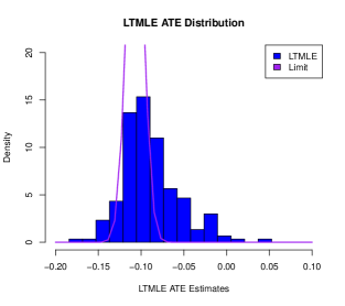
Baseline Methods for Comparison We compute these estimators with three different plug-in methods: 1) our proposed method KDPE, 2) TMLE, and 3) a baseline using the biased super-learned distribution, SL (van der Laan et al.,, 2007), which is our pre-estimate. TMLE has access to the functional form of the IF of each target parameter, and is known for its efficient limiting distribution. TMLE serves as a benchmark for examining the asymptotic efficiency of KDPE. We expect KDPE to perform no worse than TMLE. In contrast, comparisons against SL illustrate the effect of the KDPE approach on the distribution of the estimator. For DGP2, we use the longtiduinal version of TMLE, denoted as LTMLE (van der Laan and Gruber,, 2012) as our baseline. For (L)TMLE, we learn a distinct data-generating distribution for each target parameter, i.e., , to debias the estimate. KDPE and SL only use a single estimated distribution and , respectively.
Simulation Settings In all experiments, we use 300 samples () and the mean-zero Gaussian kernel. For both DGP1 and DGP2, we use hyperparameters . For DGP1, we use 450 simulations, with . For DGP2, we use 350 simulations with , 777Because larger values of result in smaller changes, we recommend setting smaller for larger .. The choice of hyperparameters are discussed in App. D.
4.4 Comparing Empirical Performance
| Method | ||||
|---|---|---|---|---|
| SL | 0.0803 | 0.2623 | 0.6796 | |
| DGP1 | TMLE | 0.0574 | 0.1723 | 0.4059 |
| KDPE | 0.0592 | 0.1752 | 0.4303 | |
| SL | 0.0508 | 0.0925 | 0.1555 | |
| DGP2 | LTMLE | 0.0731 | 0.1481 | 0.2648 |
| KDPE | 0.0295 | 0.0778 | 0.0827 |
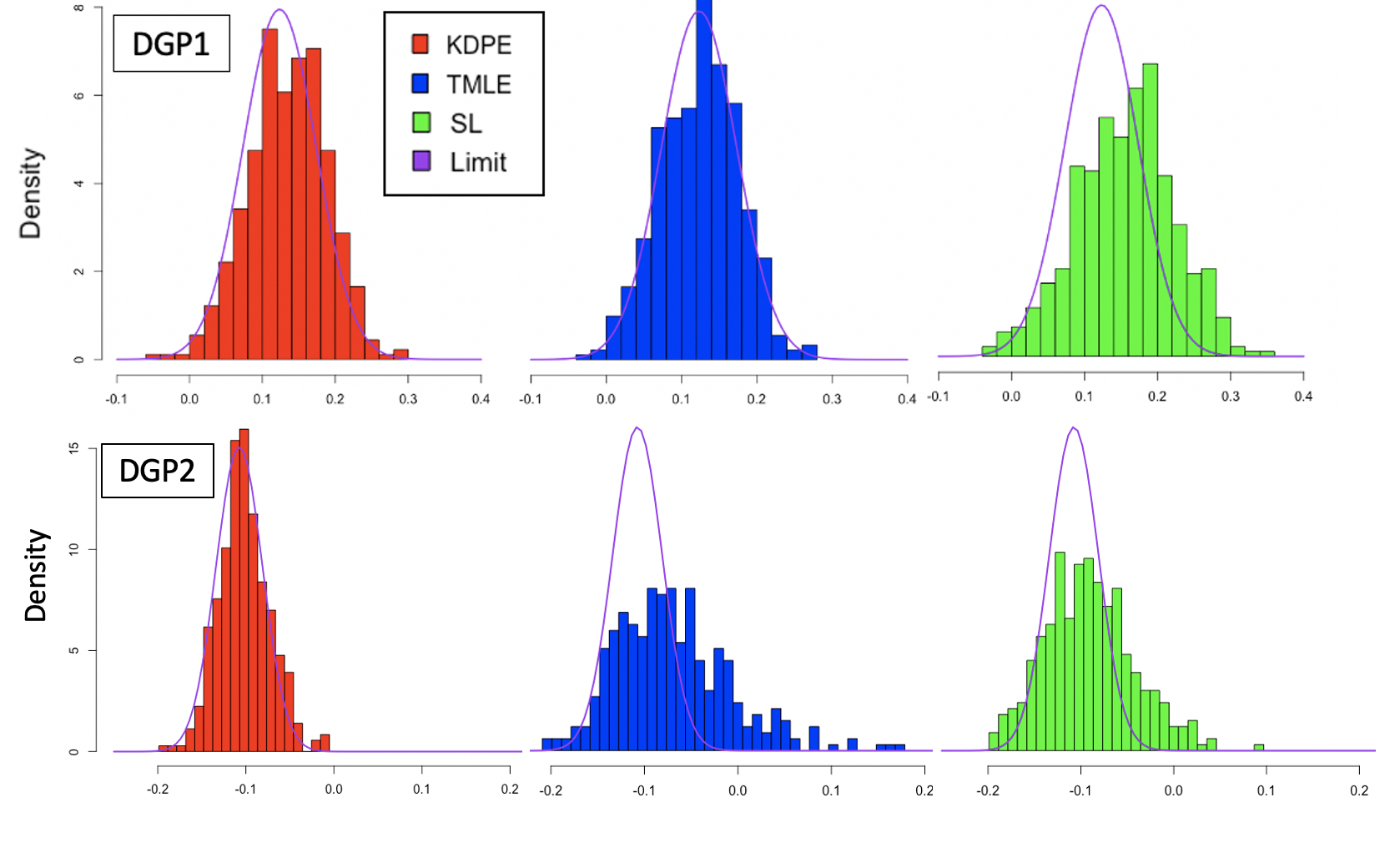
DGP1 verifies the results of Theorem 2 Our simulations for DGP1 (Figures 1 and 2) demonstrate two distinct results of Theorem 2: (i) KDPE is roughly equidistant to the efficient limiting normal distribution as TMLE, and (ii) KDPE works well as a plug-in distribution for many pathwise differentiable parameters.
As an example, the limiting distribution of is given by for DGP1. For DGP1, the distribution of in Figure 1 (and in Figure 2) highlight the necessity of debiasing. Without correction, the naive plug-in estimator deviates significantly from the limiting distribution, while both and achieve similar distributions to the limiting normal distribution. Despite no knowledge of the influence function when performing debiasing, the simulated distribution of is as close to the efficient limiting distribution as .
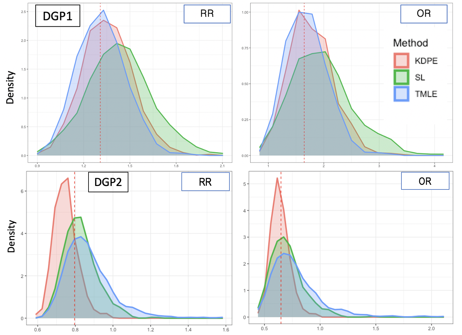
The results for DGP1 in Figure 2 verifies the second consequence of Theorem 2: for all pathwise differentiable parameters that satisfy the stated regularity conditions, is debiased as a plug-in estimator. Across all three target estimands, the distributions of perform similarly compared with TMLE, which uses a distinct targeted plug-in () for each target parameter.
DGP2 demonstrates that KDPE may provide improved finite sample performance.
DGP2 provides an example where KDPE vastly outperforms TMLE for fixed sample size , despite TMLE using the influence functions for each estimand. KDPE significantly outperforms TMLE and the naive SL plug-in estimates both in terms of RMSE, as shown in Table 1 and convergence to the asymptotic limiting distribution, as shown in Figure 1. The resulting plug-in estimates from KDPE demonstrate much smaller variance (Figures 1 and 2) than either SL or TMLE for all target parameters, and is centered correctly for . The performance of KDPE for indicates that for smaller sample sizes, KDPE may outperform a more targeted approach; in contrast, LTMLE requires a much larger sample size () to reach the correct limiting distribution.
Discussion, Limitations, and Conclusions
In this paper, we introduce KDPE, a new method for debiasing plug-in estimators that (i) does not require the IF as input, (ii) works as a general plug-in for any target parameters that satisfy our regularity conditions. Unlike existing computational IF-free debiasing methods, KDPE does not attempt to approximate the IF, retaining the simplicity of a plug-in approach.
Future work includes (i) analyzing the effect of RKHS-norm regularization on the convergence and efficiency, (ii) finding simple heuristics for setting hyperparameters , (iii) investigating how to apply sample-splitting and the extent to which it can relax our assumptions, (iv) providing primitive conditions for RKHS approximation of the IF score equation (Assumption 5), and (v) verifying the validity of bootstrap. Given the close connection between KDPE and TMLE, exploring adaptation of TMLE variants (e.g., CTMLE Coyle et al., (2023), CV-TMLE van der Laan and Rose, (2011), and one-step TMLE van der Laan and Gruber, (2016)) to KDPE for computational efficiency is worth exploring. The promising empirical performance of KDPE on DGP2 suggests that KDPE may provide better finite-sample performance. Further investigations into KDPE’s effect on the empirical process and second-order remainder terms could be pursued in future theoretical work.
Broader Impact
This paper presents work whose goal is to advance the field of Machine Learning. There are many potential societal consequences of our work, none which we feel must be specifically highlighted here.
References
- Bickel et al., (1998) Bickel, P. J., Klaassen, C., Ritov, Y., and Wellner, J. (1998). Efficient and adptive estimation for semiparametric models. Springer.
- Carmeli et al., (2010) Carmeli, C., De Vito, E., Toigo, A., and Umanitá, V. (2010). Vector valued reproducing kernel hilbert spaces and universality. Analysis and Applications, 8(01):19–61.
- Carone et al., (2018) Carone, M., Luedtke, A. R., and van der Laan, M. J. (2018). Toward computerized efficient estimation in infinite-dimensional models. Journal of the American Statistical Association.
- Chernozhukov et al., (2017) Chernozhukov, V., Chetverikov, D., Demirer, M., Duflo, E., Hansen, C., and Newey, W. (2017). Double/debiased/neyman machine learning of treatment effects. American Economic Review, 107(5):261–265.
- Chernozhukov et al., (2022) Chernozhukov, V., Newey, W. K., and Singh, R. (2022). Automatic debiased machine learning of causal and structural effects.
- Coyle et al., (2023) Coyle, J. R., Hejazi, N. S., Malenica, I., Phillips, R. V., Arnold, B. F., Mertens, A., Benjamin-Chung, J., Cai, W., Dayal, S., Colford Jr., J. M., Hubbard, A. E., and van der Laan, M. J. (2023). Targeted Learning, pages 1–20. John Wiley & Sons, Ltd.
- Fu et al., (2020) Fu, A., Narasimhan, B., and Boyd, S. (2020). CVXR: An R package for disciplined convex optimization. Journal of Statistical Software, 94(14):1–34.
- Fukumizu, (2009) Fukumizu, K. (2009). Exponential manifold by reproducing kernel Hilbert spaces, page 291–306. Cambridge University Press.
- Gruber and van der Laan, (2012) Gruber, S. and van der Laan, M. J. (2012). tmle: An R package for targeted maximum likelihood estimation. Journal of Statistical Software, 51(13):1–35.
- Hines et al., (2022) Hines, O., Dukes, O., Diaz-Ordaz, K., and Vansteelandt, S. (2022). Demystifying statistical learning based on efficient influence functions. The American Statistician, 76(3):292–304.
- Jordan et al., (2022) Jordan, M., Wang, Y., and Zhou, A. (2022). Empirical gateaux derivatives for causal inference. Advances in Neural Information Processing Systems, 35:8512–8525.
- Kennedy, (2022) Kennedy, E. H. (2022). Semiparametric doubly robust targeted double machine learning: a review. arXiv preprint arXiv:2203.06469.
- Koshevnik and Levit, (1976) Koshevnik, Y. A. and Levit, B. Y. (1976). On a non-parametric analogue of the information matrix. Teoriya Veroyatnostei i ee Primeneniya, 21(4):759–774.
- Kotz and Johnson, (1991) Kotz, S. and Johnson, N. (1991). Breakthroughs in Statistics. Number v. 1-2 in Breakthroughs in Statistics. Springer.
- Künzel et al., (2019) Künzel, S. R., Sekhon, J. S., Bickel, P. J., and Yu, B. (2019). Metalearners for estimating heterogeneous treatment effects using machine learning. Proceedings of the National Academy of Sciences, 116(10):4156–4165.
- Micchelli et al., (2006) Micchelli, C. A., Xu, Y., and Zhang, H. (2006). Universal kernels. Journal of Machine Learning Research, 7(12).
- Newey, (1990) Newey, W. K. (1990). Semiparametric efficiency bounds. Journal of Applied Econometrics, 5(2):99–135.
- Robins, (1986) Robins, J. (1986). A new approach to causal inference in mortality studies with a sustained exposure period—application to control of the healthy worker survivor effect. Mathematical Modelling, 7(9):1393–1512.
- Smale and Zhou, (2007) Smale, S. and Zhou, D.-X. (2007). Learning theory estimates via integral operators and their approximations. Constructive approximation, 26(2):153–172.
- van der Laan and Gruber, (2016) van der Laan, M. and Gruber, S. (2016). One-step targeted minimum loss-based estimation based on universal least favorable one-dimensional submodels. The international journal of biostatistics, 12:351–378.
- van der Laan et al., (2007) van der Laan, M., Polley, E., and Hubbard, A. (2007). Super learner. Technical Report Working Paper 222., U.C. Berkeley Division of Biostatistics Working Paper Series.
- van der Laan and Rose, (2011) van der Laan, M. and Rose, S. (2011). Targeted Learning: Causal Inference for Observational and Experimental Data (Springer Series in Statistics). Springer.
- van der Laan and Rose, (2018) van der Laan, M. and Rose, S. (2018). Targeted Learning in Data Science: Causal Inference for Complex Longitudinal Studies. Springer Science and Business Media.
- van der Laan et al., (2022) van der Laan, M. J., Benkeser, D., and Cai, W. (2022). Efficient estimation of pathwise differentiable target parameters with the undersmoothed highly adaptive lasso. Int J Biostat.
- van der Laan and Gruber, (2012) van der Laan, M. J. and Gruber, S. (2012). Targeted minimum loss based estimation of causal effects of multiple time point interventions. The international journal of biostatistics, 8(1).
- van der Laan and Rubin, (2006) van der Laan, M. J. and Rubin, D. (2006). Targeted maximum likelihood learning. The international journal of biostatistics, 2(1).
- van der Vaart, (1991) van der Vaart, A. (1991). On differentiable functionals. The Annals of Statistics, pages 178–204.
- van der Vaart, (2000) van der Vaart, A. (2000). Asymptotic statistics, volume 3. Cambridge university press.
- Zheng and van der Laan, (2010) Zheng, W. and van der Laan, M. (2010). Asymptotic theory for cross-validated targeted maximum likelihood estimation. Technical Report Working Paper 273., U.C. Berkeley Division of Biostatistics Working Paper Series.
Appendix
Appendix A Notation
-
set of integers
-
Sample space, with and Borel -algebra ;
-
Statistical model, collection of probability measures on ;
-
Target parameter functional, mapping from
-
Influence function, mapping from
-
Expectation functional
-
Empirical distribution function
-
The set of measurable functions
-
(Unknown) data generating distribution;
-
Represents a sequence of random variables that converges to zero in probability with respect to probability measure , at a rate that is faster than .
-
The PSD kernel and associated RKHS with kernel function
-
The function , for in support
-
Vectorized version of function , where
-
Matrix of values ,
-
The mean-zero kernel (with respect to ) and associated RKHS
-
The space of continuous functions that vanish at infinity with the uniform norm
-
A kernel is provided that is a subspace of
-
The collection of perturbations
-
The set of -dimensional parametric submodels, defined as follows:
-
The collection of perturbations corresponding to -th iteration’s distribution,
-
1-dimensional parametric model
-
RKHS-based model , where
-
Log-likelihood likelihood loss, given by
-
Derivative functional (assumed to be continuous, linear) that maps ,
for all -
The orthogonal projection operator , projects a function onto a set of functions
-
The optimal perturbation for objective function at iteration for KDPE
-
Estimated data distribution of TMLE/KDPE at iteration
-
Limiting/final estimate for TMLE/KDPE
-
Generic estimated distribution, subscripts/superscript added accordingly
-
Estimated target parameter value using plug-in distribution , subscripts/superscript added accordingly
-
Relevant portion of distribution (e.g. ).
-
An event (or set of events) such that has probability 1 under , i.e. . The standard example is the set of all possible -sample realizations from distribution .
-
The random function / distribution, indexed by events . Often, we use to index an -sample realization, , from DGP .
Appendix B Proof of Lemma 1
This expansion plays a significant role in motivating current estimation methods, such as (van der Laan and Rubin,, 2006) and (Bickel et al.,, 1998), and it also plays a crucial role in our method as well. We provide the proof for this expansion below:
Proof of Lemma 1.
We begin by revisiting a few simple results that enable this form of expansion:
-
L.1
By defining , we get that is mean zero under :
Furthermore, if is an integrable function with respect to measure , then:
-
L.2
Since is absolutely continuous with respect to , we have that :
-
L.3
Recall by the definition of , for any in the model.
Consider the first-order distributional Taylor expansion of pathwise differentiable along around (i.e., ); note that the remainder term is defined by this expansion:
| (13) |
Then, we subtract the following zero term in our expansion
Collecting terms, multiplying by and setting leads to:
| (2) |
∎
Appendix C KDPE Theory
C.1 Proof of Proposition 1
Proof of Proposition 1.
Because is bounded, the expectation functional is continuous on . Next, we note that and it is the Riesz representer of the expectation functional (we have shown this elsewhere and remark here that the rigorous argument considers a Riemann approximation to the expectation integral and weakly convergent subsequences). It follows that if and only if , and from this we can deduce the projection operator onto and the reproducing kernel of that subspace.
Finally, given , let be an approximating sequence of in . Let be the RKHS orthogonal decomposition of into and , and note that this operation is continuous on . By continuity of expectation in , in . It follows that the orthogonal part of vanishes in and in . Thus, is dense in . ∎
C.2 Proof of Theorem 1
Let be a general loss function that identifies the relevant part, , for the target parameter of interest , satisfying the property that for every possible . The log-likelihood is a special case of such a loss function. The risk associated with the log-likelihood identifies the entire distribution based on the properties of the Kullback–Leibler divergence.
Proof of Theorem 1.
For consider the orthogonal decomposition into the closed subspaces and . From the reproducing property it follows that and for every . This means that inputs and yield the same value of the empirical risk in the objective function of (6). Furthermore, we have assumed that if is admissible in the optimization problem (6), then so is . The claim follows by noting that . ∎
C.3 Proof of Proposition 2
Remark 2.
Assumption 3 assumes that our algorithm converges and terminates in finite time. It is important to highlight that this assumption is commonly adopted in the TMLE literature (van der Laan and Rubin,, 2006). As demonstrated in Table 2, our algorithm, Algorithm 10, converges effectively in practice, typically requiring only a few iterations. While the regularization of the perturbation size (i.e., the norm of ) could potentially ensure finite convergence, it is beyond the scope of this paper and remains a topic for future research.
Proof of Proposition 2.
This follows from the first order condition to (6) which must hold at the interior local minimum. First, consider the variations at in along the directions (scores) given by and observe:
This shows that the estimating equation holds for each of these scores, and therefore their linear combinations. Second, by Theorem 1, any that is orthogonal to these scores must have for all and therefore satisfy Equation (12). From these two observations, we conclude the proposition. ∎
C.4 Proof of Theorem 2
Remark 3.
Assumptions 2-3 and conclusions derived from them are standard in the TMLE literature (van der Laan and Rubin,, 2006; Kennedy,, 2022). Assumption 4 is mostly technical and ensures that the set of scores that satisfy the estimating equation (12) is sufficiently rich to achieve debiasing for the target parameter by approximating its efficient influence curve estimating equation asymptotically.
Assumption 5 is our main regularity assumption on the model and functional needed to control the plug-in bias term of the proposed KDPE estimator. While this assumption provides a clear intuition for the debiasing mechanism of KDPE, it is not strictly required for the method to work. Less extreme conditions on the regularity of , such as or Sobolev norm bounds (see van der Vaart, 2000, Ch 19 and RKHS approximation theory Smale and Zhou, 2007), can imply the Donsker property in S5.
The Donsker assumption S2 has been successfully relaxed for related estimators in the literature (Zheng and van der Laan,, 2010; Kennedy,, 2022; Chernozhukov et al.,, 2017) via sample-splitting. Our initial analysis of DKPE crucially relies on the Donsker assumption in the argument for asymptotic debiasing (based on S5). We leave the analysis of KDPE with sample-splitting (as done in Zheng and van der Laan, 2010) to future work.
Proof of Theorem 2.
The density of RKHS in for the norm follows if the projection operator is continuous with respect to the norm by the argument given in Proposition 1. The latter continuity holds if the expectation functional is a continuous in -norm, which follows from by Cauchy-Schwarz inequality.
Appendix D Simulation Details and Additional Empirical Results
This section provides pseudocode for the bootstrap procedure, empirical justification for our choice of hyperparameters , and additional experiments for the bootstrap variance estimation procedure. All simulations were performed on a Dell Desktop with 11th Gen Intel Core i7, 16 GB of RAM. All code for the simulations provided in both this section and Section 4 can be found on https://github.com/anonymous/KDPE.
D.1 Baseline Methods
Initializing for KDPE
For all simulations, we use the SuperLearner (van der Laan et al.,, 2007) and tmle, ltmle (Gruber and van der Laan,, 2012; van der Laan and Gruber,, 2012) packages in R. For SuperLearner, we set our initial base learners as SL.randomForest, SL.glm, and SL.mean. For tmle, ltmle, we use the default settings, except for setting the parameter g.bound to 0. For each run of the simulations, we initialize for both TMLE and KDPE to the same initial density estimate to capture the differences in the two debiasing approaches.
Optimization Step Details
For the optimization solver, we use the package CVXR (Fu et al.,, 2020) with the default settings to obtain , which corresponds to the parametric update step in Algorithm 10. Because the log-likelihood loss function is concave and all constraints are linear, our update step can be solved by existing convex optimization software. To avoid solvers, a potential future direction is to explore alternative loss functions that have known closed-form solutions, such as the mean squared error (MSE), rather than using the log-likelihood loss.
Construction of
To construct our -dimensional parametric submodels, we use the mean-zero RBF kernel , which takes the following form:
where . Following classical examples (van der Laan and Rose,, 2018) and existing software (Gruber and van der Laan,, 2012) for TMLE, we fix and (the initial estimate for the propensity score function). This enables us to directly calculate the integral, rather than approximate :
| (14) |
where and are defined as follows:
Note that this calculation is inherent to our setting of binary treatments and outcomes with the empirical marginal distribution for – other set-ups may not permit a direct calculation of the integral, and may require integral approximations. We defer those experiments to future work.
D.2 Update Steps for Simulations
To get the specific updates for DGP1, DGP2, we project the chosen score (i.e., ) into the relevant tangent space. The only change in Algorithm 1 is the following step, which occurs at the end of each loop:
For all set-ups in our simulation, the tangent space factorizes nicely, which means we simply need to project our chosen score at each iteration. We demonstrate the necessary modifications to obtain our results.
DGP1
Since the conditional density function does not show up in the expression of our final plug-in estimate of the target parameters (ATE, RR, OR), it suffices to consider only updating the conditional density function , with distribution fixed. The tangent space decomposes as follows:
where is space of scores (i.e., directions of change) corresponding to . To obtain the component of our chosen score relevant for , we simply project this into :
DGP2
Similarly, since and do not show up in the expression of our final plug-in estimate of the target parameters, we do not need to update these components. We fix the marginal distribution of baseline covariates as . The two components relevant for our target parameters are , and . The tangent space for DGP2 factorizes as follows:
where and are the corresponding tangent spaces for and respectively. At the end of each iteration, we project the chosen score into the tangent space of these relevant components, and update accordingly:
D.3 Hyperparameter Testing for KDPE
Density Bound and Convergence Criteria
In our experiments, we fixed the sample size at . We conducted tests with different values for the density bound , with , and for the stopping criteria, we tested for DGP1, with fixed at . For each combination of settings, we performed 100 simulations to obtain the results presented in Table 2 and Figure 3.
| ATE RMSE | RR RMSE | OR RMSE | Avg. Iterations | ||
|---|---|---|---|---|---|
| 0.050 | 0.025 | 0.019 | 0.077 | 0.205 | 1.062 |
| 0.010 | 0.025 | 0.016 | 0.063 | 0.180 | 1.135 |
| 0.002 | 0.025 | 0.026 | 0.101 | 0.260 | 1.120 |
| 0.050 | 0.005 | 0.015 | 0.057 | 0.150 | 2.293 |
| 0.010 | 0.005 | 0.004 | 0.026 | 0.091 | 2.445 |
| 0.002 | 0.005 | 0.006 | 0.033 | 0.090 | 2.505 |
| 0.050 | 0.001 | 0.001 | 0.023 | 0.068 | 4.756 |
| 0.010 | 0.001 | 0.009 | 0.040 | 0.128 | 5.329 |
| 0.002 | 0.001 | 0.009 | 0.033 | 0.105 | 5.802 |
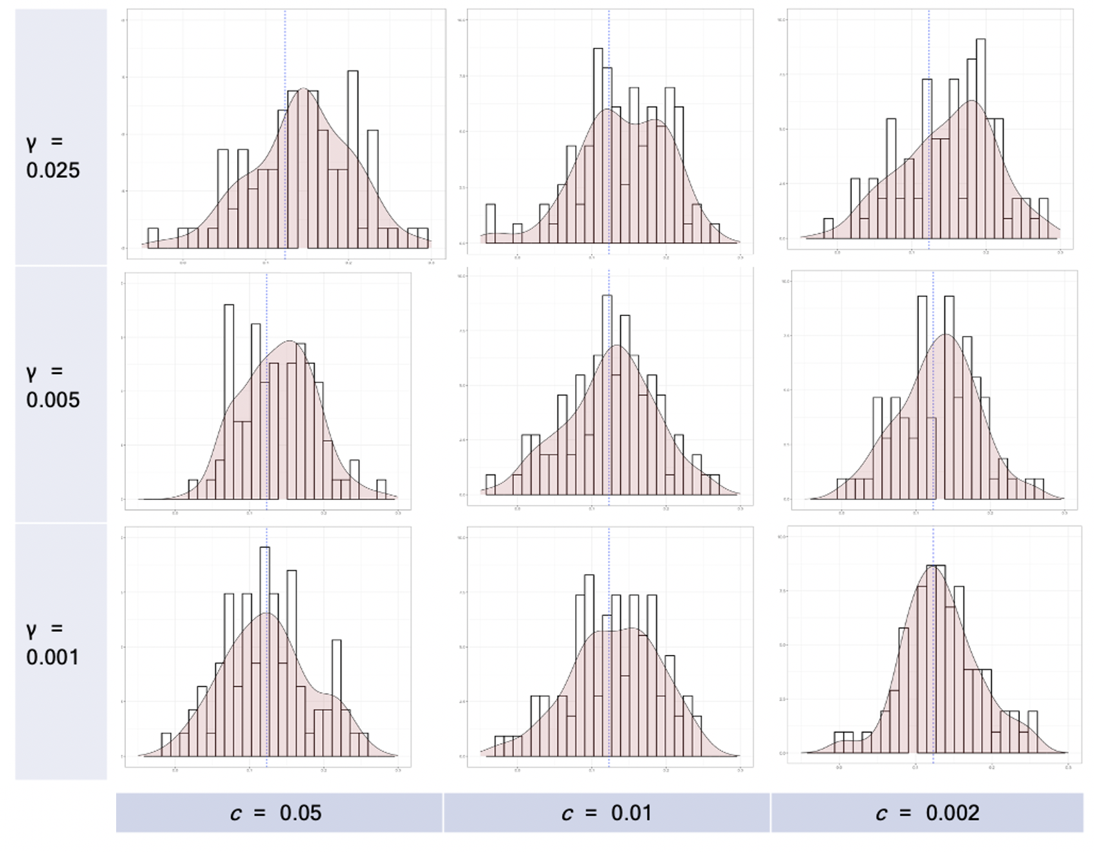
The empirical results shown in Figure 3 coincide with the theoretical results shown in Appendix C, which are derived under the setting where we have no explicit density bound and we terminate at a fixed point . As we see in Figure 3, the simulated distribution of with the smallest tested values of obtains a distribution most similar to limiting normal distribution. When the density bound is set to large values (e.g., ), the resulting distributions become skewed and deviate significantly from the normal distribution. This occurs because termination at the boundary (i.e., is tight with respect to the density bound) prevents the distributions from satisfying the gradient conditions shown in Appendix C. When using large values for the convergence tolerance (e.g., ), the algorithm terminates prematurely at a distribution that deviates significantly from the fixed point . Thus, to maintain the guarantees shown in Appendix C for Algorithm 1, we want the values of to be as small as possible. For DGP1 in Sections 4.4, we opt for , values at least as small as the tested hyperparameter values. The results of this simulation naturally pose questions of how to set as functions of , such that the residual bias caused by these hyperparameters is . This remains an open question for future work.
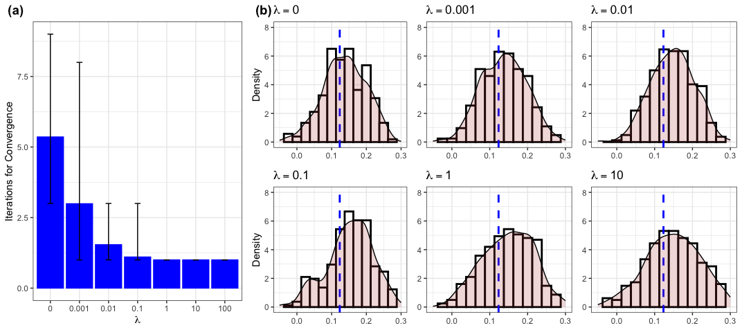
Regularization Parameter
While the theoretical guarantees of KDPE hold for any , the choice of has practical significance, especially in relation to the convergence tolerance parameter . Large values of (i.e., looser convergence tolerances) with heavy regularization (i.e., large ) results in premature termination. We demonstrate these results with DGP1, testing 888Note that for , which we use throughout our paper, the solver CVXR fails to obtain a solution roughly 15% of the time. For those interested in testing the code, we recommend , which results in similar results, but avoids numerical instability issues.. For each , we ran 100 simulations with to determine the best choice of . As shown in Figure 4, for a fixed value of convergence tolerance , we see that larger values of tend to result in skewed distributions and/or heavy tails. The average iterations for convergence corroborate that this is due to premature termination; the resulting step with heavy regularization results in a relatively small change in distribution and trivially satisfies our convergence criteria. For this reason, for DGP2 (which uses ), we set the convergence tolerance to , as compared to in the non-regularized case in DGP1. We keep the density bound for DGP2 the same (). Future extensions of this work include how to set regularization parameter as a function of convergence tolerance .
D.4 Additional (L)TMLE Results for DGP2
We provide additional results to show that the poor performance of TMLE in DGP2 is due to the relatively small sample size . For , Figure 5 see that the distribution of is far closer to the limiting distribution (shown in purple) than when , as shown in the main body of our paper. This indicates that the performance of TMLE for DGP2 at is indeed due to poor finite sample performance.
D.5 Runtime Complexity for KDPE
Our algorithm is a meta-algorithm, and thus the computational complexity is dependent on different factors (integration method, optimization software, number of iterations, etc.). We provide computational complexity results per iteration in the case of Algorithm 1. The set-up necessary to formulate the optimization problem requires us to obtain (Eq. 20) for all , and occurs the cost :
-
•
Computing for all :
-
•
Computing for all :
-
•
Computing :
The optimization problem for KDPE involves regressors, and therefore the computational complexity of this method is per iteration, where is the complexity for the solver.
In contrast, TMLE (as introduced in the paper) occurs an cost when calculating the influence function in each iteration, and involves only 1 regressor, resulting in a complexity of in each iteration.
The difference in cost per iteration (quadratic, as opposed to linear in ), can be seen as the price to pay for a plug-in distribution that works with all parameters satisfying our regularity assumptions. Our empirical results corroborate these scaling results. The median time-per-iteration in DGP1 for 150 samples and 300 samples is 0.22 and 0.91 respectively, indicating a roughly scaling for our method. For DGP1, we average between 5-6 iterations before termination, using the hyperparameters in Section 4. For DGP2, we average 2 iterations before termination. Across our simulations for DGP1, the average runtime for our method is 5.8 seconds, with 5.8 iterations on average. TMLE, as implemented in (van der Laan and Gruber,, 2016), uses the one-step method, which performs the MLE optimization in one iteration using logistic regression. Because this version of TMLE involves no iterations (same time complexity as logistic regression), it is a poor comparison with KDPE in terms of time complexity. The results of TMLE are included as a standard of comparison for the distribution of our estimator, rather than its time complexity.
D.6 Bootstrap Algorithm
We use the classical bootstrap procedure (Kotz and Johnson,, 1991), i.e., sampling observations from our observed data with replacement, to estimate the variance of the estimator. We formally state this procedure in Algorithm 2.
D.7 Bootstrap Intervals for Inference
| Parameter | Avg. Length (95% CI) | Coverage (95% CI) | ||
|---|---|---|---|---|
| KDPE | 0.00427 (0.00287) | 0.252 | 0.945 | |
| 0.04562 (0.02555) | 0.826 | 0.975 | ||
| 0.30303 (0.15322) | 2.107 | 0.970 | ||
| TMLE | 0.00192 (0.00296) | 0.172 | 0.903 | |
| 0.01483 (0.02837) | 0.510 | 0.903 | ||
| 0.07016 (0.14981) | 1.230 | 0.907 |
Table 3 reports average estimated variance, average length of 95% intervals, and the coverage across 237 simulations of for DGP1. For comparison, we include the results of inference for TMLE, which estimates the variance using knowledge of the (efficient) IF. The baselines for both TMLE and KDPE (in parentheses) are the sample variances of the simulated distributions in Section 4.4, and provided next to average estimated variance. The KDPE-bootstrap variance estimates overestimate the variance for all target parameters relative to the KDPE baseline; the inflated variance estimates lead to conservative confidence intervals for the bootstrapped KDPE estimates with over-coverage, as shown in the coverage results of Table 3. By contrast, TMLE’s IF-based variance estimate underestimates the variance for all target parameters relative to the TMLE baseline, leading to undercoverage. These preliminary results suggest that bootstrap interval calibration is future direction for improvement, and are intended as a starting point for future investigation. While these results imply that our bootstrap-estimated confidence intervals are conservative, more extensive testing is required to empirically validate these results. A large theoretical gap also remains for confirming that our bootstrap-estimated variances are consistent asymptotically, and providing an analysis for Algorithm 2 under KDPE is another natural step towards our goal of fully computerized inference. Lastly, as shown in Table 3 and Algorithm 2, we only use the bootstrap samples to estimate the variance of our estimator and use a normal approximation to construct confidence intervals. Alternative methods for constructing confidence intervals include directly taking the quantiles of the bootstrap estimates and/or subsampling while bootstrapping, which we do not explore in this project.