Quantum interference effects in a $\Lambda$-type atom interacting with two short laser pulse trains

Abstract

We study the quantum interference between the excitation pathways in a three-level $\Lambda$-type atom interacting with two short laser pulse trains under the conditions of electromagnetically induced transparency. The probability amplitude equations which describe the interaction of a three-level $\Lambda$-type atom with two laser pulse trains are numerically solved. We derive analytical expressions for the population of the upper excited state for resonant laser pulse trains with a rectangular temporal profile. By varying the parameters of the laser pulse trains such as area of a single pulse, detuning, repetition period, and number of individual pulses, we analyze the quantum interference between the excitation pathways in terms of the upper excited state population.

1 Introduction

Due to the important development of the laser sources, quantum control (sometimes referred to as optimal control or coherent control) has become of increasing interest in the last years in both physical and chemical sciences. Quantum control aims at manipulating the course of the quantum dynamics of atomic or molecular systems and is based on quantum interferences. Up to now three methods have been proposed in order to achieve quantum control: the temporal coherent control that uses the temporal quantum interference of laser fields, optimal control that uses the techniques of pulse shaping, and adiabatic passage in order to realize a complete population transfer between two quantum states Shapiro2000 ; Ehlotzky .

Through the quantum interference between two different excitation pathways the optical response of an atomic medium could be modified and an opaque optical medium can be rendered transparent to a probe field by applying an intense coupling laser field Harris ; Marangos ; Bergmann . This effect is named electromagnetically induced transparency (EIT) and represents a coherent optical nonlinearity which renders a medium transparent over a narrow spectral range within an absorption line. The absorption peak is split and both absorption and refraction index vanish at resonance. The EIT was theoretically proposed by Kocharovskaya et al. Olga and then it was experimentally observed in Sr Boller . Since its observation, EIT has been intensively studied and developed in the domain of lasing without inversion, nonlinear optics, sub-fs pulse generation, atomic coherence control, slow light, giant nonlinear effect, storage of light, etc. Fleischhauer . The basis of the EIT phenomena resides in the coherent population trapping (CPT) Bergmann that was for the first time discovered by Alzetta et al. Alzetta in the D lines of the Na atom. Thus for a three-level $\Lambda$-type atom interacting with a probe and a coupling laser, the population is trapped in the lower states and the population of the upper excited state is negligible. In terms of quantum interference, the contributions to the probability amplitude of the upper state from the two lower states interfere destructively and the population of the upper state could become negligible and therefore the laser radiation is not absorbed. This quantum interference can be created among different quantum paths reaching the same final state with single laser pulses or by several consecutive mutually coherent laser pulses: namely a laser pulse train. By using a laser pulse train ultrahigh resolution spectroscopy, with the comb linewidths much smaller than the bandwidth of the pulse, can be obtained. Lately, it has been shown that the coherent accumulation effects of populations and atomic coherences play a role in the coherent control of atomic or molecular systems with laser pulse trains Marian ; Stowe . Most of the latest studies regarding the coherent accumulation effects in a three-level atom excited by a fs laser pulse train are done either in the simplified hypothesis of a stationary state Felinto2003 or in the weak field limit, within the lowest order perturbation theory Felinto2004 . By properly adjusting the amplitudes and phases of the pulses, the coherent excitation of a two-level system with a train of ultrashort laser pulses reproduces the effect normally achieved with a single frequency-chirped pulse Shapiro2008 . The effect of the pulse area and the number of pulses of a train of ultrashort pulses was also investigated for a two-level atom Nakajima2008 . Recently, EIT and Autler-Townes splitting were studied for an ultrashort train pulse interacting with a $\Lambda$-type atom driven by a continuous wave (CW) laser Soares2010 . The coherent population trapping has been investigated with a train of ultrashort pulses of rectangular pulse shape in the steady-state or weak field regime viana2011 . Very recently, the dynamics of a $\Lambda$-type atom interacting with non-overlapping ultrashort laser train pulses with a delta-function temporal dependence of the individual pulses was studied in Ilnova .

In this paper we study the quantum interference between the excitation pathways in a $\Lambda$-type atom interacting with two trains of laser pulses under the EIT conditions. As specified before, under the conditions of EIT a medium could become transparent for a probe laser by introducing a second laser: coupling laser which is, usually, much stronger than the probe laser. We assume interaction with two short laser pulse trains, with short repetition periods, such that the atom does not have enough time to completely relax between two consecutive single pulses and therefore we expect some coherent accumulation effects during the propagation. The paper is organized as follows. In Section 2 we present the theoretical model. The time-dependent Schrödinger equation which describes the interaction of a $\Lambda$-type atom with a probe and a coupling laser pulse train is numerically solved. Analytical results are presented for a particular case of laser trains with rectangular pulse shape. In Section 3 we present illustrative results for the interaction of two short probe and coupling laser pulse trains with a $\Lambda$-type atom, for a coupling laser stronger than a probe laser. We examine the effect of the parameters of the laser pulse trains such as pulse area, laser detunings, and number of individual pulses, on the quantum interference in terms of the upper excited state population. Finally, concluding remarks are given in Section 4. Atomic units are used throughout this paper unless otherwise mentioned.

2 Theoretical approach

2.1 The time-dependent probability amplitude equations

It is well known that many atomic processes could be considered as involving only few levels and using a three-level $\Lambda$ model atom provides a simple and realistic description of the physical processes. Our system under consideration is a three-level $\Lambda$-type atom interacting with two laser fields: The states $|1\rangle$ and $|2\rangle$ are coupled by a probe laser $\bm{\mathcal{E}}_{p}(t)$ with photon energy $\omega_{p}$, while the states $|2\rangle$ and $|3\rangle$ are connected by a coupling laser $\bm{\mathcal{E}}_{c}(t)$ with photon energy $\omega_{c}$. The probe and coupling lasers are tunned near resonance with the respective transitions, and the transition between the states $|1\rangle$ and $|3\rangle$ is dipole-forbidden. Both the probe and coupling laser pulses are considered as laser pulse trains and are described by an electric field which can be written as a sum of equally spaced identical electric fields

$$\bm{\mathcal{E}}_{j}(t)=\mathcal{E}_{0j}\;\bm{e_{j}}\;e^{i\omega_{j}t}\sum_{q=0}^{N-1}f_{j}(t-qT_{j})e^{iq\phi}+c.c.,$$ (1)

where $\mathcal{E}_{0j}$ is the peak amplitude of the electric field ($j=p$ or $c$ and hereafter), $\bm{e_{j}}$ is the polarization vector, and $f_{j}(t)$ is the slowly varying envelope. $T_{j}$ is the laser pulse repetition period that represents the time separation between two successive single pulses, $N$ is the number of individual pulses in the train pulse, and $\phi$ is the phase shift between the two successive pulses. We assume both probe and coupling fields are linear polarized in the same direction, with the same pulse repetition period $T$ and the phase shift $\phi$ is neglected. We consider that both probe and coupling lasers have the same time dependence, with the temporal envelope of each single pulse in the train described by a Gaussian function

$$f_{j}(t)=e^{-\pi\left({t}/{\tau_{j}}\right)^{2}},$$ (2)

where $\tau_{j}$ is the temporal width of a single laser pulse.

By taking the Fourier transform of the electric field, equation (1), with respect to time as

$$\mathcal{\widetilde{E}}_{j}(\omega)=\int_{-\infty}^{+\infty}\mathcal{E}_{j}(t)e^{-i\omega t}dt,$$ (3)

where the symbol $\sim$ denotes the Fourier transform, we obtain, after simple algebra,

$$\mathcal{\widetilde{E}}_{j}(\omega)=\mathcal{E}_{0j}\widetilde{f}_{j}(\omega-\omega_{j})\frac{1-\exp{(iN\omega T)}}{1-\exp{(i\omega T)}}.$$ (4)

The intensity of the laser pulse train in the frequency domain is calculated as

$$I_{j}(\omega)=|\mathcal{\widetilde{E}}_{j}(\omega)|^{2}={I}_{0j}(\omega)\sin^{2}\left(\frac{N\omega T}{2}\right)\sin^{-2}\left(\frac{\omega T}{2}\right),$$ (5)

where $I_{0j}(\omega)=|2\pi\mathcal{E}_{0j}/T|^{2}\left|\widetilde{f}_{j}(\omega-\omega_{j})\right|^{2}$ represents the laser intensity of a single pulse. In the limit of $N\to\infty$ we obtain, after a simple calculation,

$$I_{j}(\omega)={I}_{0j}(\omega)\sum_{N=-\infty}^{+\infty}\delta(\omega-\omega_{jN}),$$ (6)

where $\omega_{jN}=\omega_{j}+N\omega_{r}$. The frequency spectrum of the electric field given by equation (1) consists of a comb of $N^{th}$ laser modes that are separated by the repetition angular frequency $\omega_{r}=2\pi/T$ and centered at $\omega_{j}$. The photon energy of the $N^{th}$ mode of laser pulse train is given by $\omega_{j}\pm N\omega_{r}$.

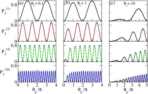
Figure 1: (Color online) Population of the upper excited state $P_{2}^{(N)}$ as a function of the probe laser area. The solid lines show the numerical results while the solid circles shows the analytical results. The number of individual pulses in the trains are $N=1,2,4,$ and $10$ (from top to bottom). The coupling laser area $\theta_{c}$ is $0.1$ in (a), $1$ in (b), and $10$ in (c). Both laser pulse trains have a Gaussian temporal envelope with the duration $\tau=1$ ps, repetition period $T=1$ ns, and $\delta_{p}=\delta_{c}=0$. The spontaneous decay rate is $\gamma=70$ MHz which results in the value $\gamma T=0.07$.

In order to study the temporal evolution of the atomic system we derive the time dependent Schrödinger equation for the interaction of a $\Lambda$-type atom with the probe and coupling lasers in the standard framework of rotating wave approximation, as long as the pulse duration is not very short (e.g. not in the fs time domain). For simplicity reasons the Doppler broadening of the atomic levels is not included in the calculation. By using the standard procedure, we obtain the following set of time-dependent probability amplitude equations for the interaction of the $\Lambda$-type atom, as illustrated in Figure 1, with the probe and coupling lasers given by equation (1)

$$\frac{\partial}{\partial t}{u}_{1}(t) = \;\frac{i}{2}{\Omega}_{p}(t)u_{2}(t),$$ (7)

$$\frac{\partial}{\partial t}{u}_{2}(t) = -(i\delta_{p}+\gamma)u_{2}(t)+\;\frac{i}{2}{\Omega}_{p}(t)u_{1}(t)$$ (8)

$$+\;\frac{i}{2}{\Omega}_{c}(t)u_{3}(t),$$

$$\frac{\partial}{\partial t}{u}_{3}(t) = -i(\delta_{p}-\delta_{c})u_{3}(t)+\;\frac{i}{2}{\Omega}_{c}(t)u_{2}(t),$$ (9)

where ${u}_{k}(t)$ is the slowly varying probability amplitude of state $|k\rangle$ ($k=1,2$, and $3$) that satisfies the initial conditions ${u}_{1}(t=-\infty)=1$ and ${u}_{k}(t=-\infty)=0$ ($k=2$ and $3$). Here $\Omega_{p}(t)$ and $\Omega_{c}(t)$ are the one-photon Rabi frequency due to the probe and coupling lasers, which are defined as

$${\Omega}_{p}(t)={\Omega}_{0p}\sum_{q=0}^{N-1}f_{p}(t-qT),$$

$${\Omega}_{c}(t)={\Omega}_{0c}\sum_{q=0}^{N-1}f_{c}(t-qT),$$

with the magnitudes ${\Omega}_{0p}=d_{12}{\mathcal{E}}_{0p}$ and ${\Omega}_{0c}=d_{23}{\mathcal{E}}_{0c}$, where $d_{12}$ is the one-photon dipole moment for the transition between states $|1\rangle$ and $|2\rangle$, and $d_{23}$ is the one-photon dipole moment for the transition between the states $|2\rangle$ and $|3\rangle$. $\delta_{p}$ and $\delta_{c}$ are the one-photon detunings from the resonance of the probe and coupling lasers, respectively, and $\gamma$ is the spontaneous decay rate of the upper excited state $|2\rangle$. We introduce the temporal area of a single pulse, defined as the integral of the Rabi frequency over time

$$\theta_{j}=\Omega_{0j}\int_{-\infty}^{\infty}f_{j}(t)dt\quad\text{($j=p$ or $c$)}.$$ (10)

For a laser pulse train with the Gaussian temporal envelope given by equation (2), the area of a single pulse is obtained after a straightforward algebra as $\theta_{p}=\Omega_{0p}\tau_{p}$ for the probe laser and $\theta_{c}=\Omega_{0c}\tau_{c}$ for the coupling laser.

For laser pulses with arbitrary pulse envelopes and off-resonant photon energies, when damping is included, a general analytic solution of equations (7)-(9) cannot be derived. Therefore we numerically integrate equations (7)-(9) for realistic atomic and lasers parameters. In order to understand the numerical results and the dynamics of the system we analyze in the next subsection the particular case of two resonant laser pulse trains with rectangular envelopes and the same temporal pulse areas as those given by the Gaussian envelope equation (2).

2.2 Analytic solutions for resonant probe and coupling laser pulse trains

We analytically solve the set of three nonlinear coupled differential equations (7)-(9) and derive an analytical solution for the population of the upper excited state $|2\rangle$. We consider a probe and a coupling laser pulse train that are one-photon resonant with the $|1\rangle-|2\rangle$ and $|2\rangle-|3\rangle$ transitions, respectively, $\delta_{p}=\delta_{c}=0$.

For simplicity, we assume laser pulse trains with rectangular pulse envelopes of temporal width $\tau_{p}=\tau_{c}=\tau$, for both probe and coupling lasers, with the following one-photon Rabi frequency

$$\Omega_{j}(t)=\begin{cases}\Omega_{0j},&\quad\text{for \; $qT\leq t\leq\tau+qT$},\\ 0,&\quad\text{for \; $\tau+qT\leq t\leq\tau+(q+1)T$},\end{cases}$$

where $0\leq q\leq N-1$ and $j=p$ or $c$. Since the atom interacts with two different laser fields we define the total Rabi frequency as the root mean square of the probe and coupling Rabi frequencies $\Omega_{0}=(\Omega_{0p}^{2}+\Omega_{0c}^{2})^{1/2}$. It is worth mentioning that for resonant photon energies the transition probability depends on the temporal pulse area only and is almost insensitive to the temporal envelope of the laser pulse Shore . Here the temporal areas of each single probe and coupling pulse are $\theta_{p}=\Omega_{0p}\tau_{p}$ and $\theta_{c}=\Omega_{0c}\tau_{c}$, respectively, and are identical with those areas for probe and coupling pulses with Gaussian temporal envelopes given by equation (2).

Now for $\gamma<\Omega_{0}$, which is often the case, equations (7)-(9) can be easily solved for the first pulse in the train ($N=1$), $0\leq t\leq\tau$, and the population of the upper excited state at the end of the first pulse reads as

$$P_{2}^{(1)}=|u_{2}^{(1)}(\tau)|^{2}=\frac{\Omega_{0p}^{2}}{\Omega^{2}}\;e^{-\gamma\tau}\;\sin^{2}\left(\frac{\theta}{2}\right),$$ (11)

where $\theta=\Omega\tau$ represents the effective temporal pulse area of a single pair of probe and coupling pulses and $\Omega$ is the effective Rabi flopping frequency

$$\Omega=(\Omega_{0}^{2}-\gamma^{2})^{1/2}\qquad(\gamma<\Omega_{0}).$$

Next, after a straightforward algebra we obtain the population of the upper excited state $|2\rangle$ at the end of the 2^nd ($N=2$), 3^rd ($N=3$), and 4^th ($N=4$) pulse, respectively, calculated for $\gamma<\Omega_{0}$ as

$$P_{2}^{(2)} = \left|u_{2}(\tau+T)\right|^{2}=4\;P_{2}^{(1)}e^{-\gamma T}$$

$$\times \left[\cos\left(\frac{\theta}{2}\right)\cosh\beta+\frac{\gamma}{\Omega}\sin\left(\frac{\theta}{2}\right)\sinh\beta\right]^{2},$$

$$P_{2}^{(3)} = \left|u_{2}(\tau+2T)\right|^{2}=16\;P_{2}^{(1)}e^{-2\gamma T}$$

$$\times \left\{\left[\cos\left(\frac{\theta}{2}\right)\cosh\beta+\frac{\gamma}{\Omega}\sin\left(\frac{\theta}{2}\right)\sinh\beta\right]^{2}-\frac{1}{4}\right\}^{2},$$

$$P_{2}^{(4)} = \left|u_{2}(\tau+3T)\right|^{2}=64\;P_{2}^{(1)}e^{-3\gamma T}\cos^{2}\left(\frac{\theta}{2}\right)\cosh^{2}\beta$$ (14)

$$\times \left[\cos^{2}\left(\frac{\theta}{2}\right)\cosh^{2}\beta-\frac{1}{2}\right]^{2}\qquad(\gamma\ll\Omega_{0}),$$

where the argument of the hyperbolic functions is $\beta={\gamma\;(T-\tau)}/{2}$. After the interaction of the $\Lambda$-type atom with a train of $N$ probe and coupling pulses, for $\gamma\ll\Omega_{0}$, we obtain the following analytical formula for the population of the upper excited state at the end of the $N^{th}$ pulse

$$P_{2}^{(N)} = \left|u_{2}[\tau+(N-1)T]\right|^{2}=0.25\;P_{2}^{(1)}\;e^{-(N-1)\gamma T}$$ (15)

$$\times \left|\left[\cos^{2}\left(\frac{\theta}{2}\right)\cosh^{2}\beta+i\sqrt{1-\cos^{2}\left(\frac{\theta}{2}\right)\cosh^{2}\beta}\right]^{N}\right.$$

$$- \left.\left[\cos^{2}\left(\frac{\theta}{2}\right)\cosh^{2}\beta-i\sqrt{1-\cos^{2}\left(\frac{\theta}{2}\right)\cosh^{2}\beta}\right]^{N}\right|^{2}$$

$$\times \left|1-\cos^{2}\left(\frac{\theta}{2}\right)\cosh^{2}\beta\right|^{-1}\quad(\gamma\ll\Omega_{0}).$$

In the limit of short laser pulses and small decay rate compared with the pulse repetition frequency and the comb width ($\gamma T\ll 1$ and $\gamma\tau\ll 1$), for $\gamma\ll\Omega_{0}$, equations (11)-(14) further simplify as

$$P_{2}^{(1)}\simeq\frac{1}{1+\Omega_{0c}^{2}/\Omega_{0p}^{2}}\;\sin^{2}\left(\frac{\theta}{2}\right),$$ (16)

$$P_{2}^{(2)}\simeq\frac{e^{-\gamma T}}{1+\Omega_{0c}^{2}/\Omega_{0p}^{2}}\;\sin^{2}\left(\theta\right),$$ (17)

$$P_{2}^{(3)}\simeq\frac{e^{-2\gamma T}}{1+\Omega_{0c}^{2}/\Omega_{0p}^{2}}\;\sin^{2}\left(\frac{3\theta}{2}\right),$$ (18)

$$P_{2}^{(4)}\simeq\frac{e^{-3\gamma T}}{1+\Omega_{0c}^{2}/\Omega_{0p}^{2}}\;\sin^{2}\left(2\theta\right).$$ (19)

Furthermore, the population of the upper excited state $|2\rangle$ at the end of the $N^{th}$ pulse, $P_{2}^{(N)}$, equation (15), could be easily expressed as

$$P_{2}^{(N)} \simeq P_{2}^{(1)}\;e^{-(N-1)\gamma T}\;\sin^{2}\left(\frac{N\theta}{2}\right)\sin^{-2}\left(\frac{\theta}{2}\right)$$ (20)

$$= \frac{e^{-(N-1)\gamma T}}{1+\Omega_{0c}^{2}/\Omega_{0p}^{2}}\;\sin^{2}\left(\frac{N\theta}{2}\right).$$

It is worth pointing out that equation (20) resembles equation (5) that describes the intensity of the laser pulse train in the frequency domain.

The simplified equations (16)-(20) clearly show that the number of pulses, the accumulated effective pulse area $N\theta$, the repetition period, the spontaneous decay rate, and the ratio of the probe and coupling Rabi frequencies play an important role in the accumulation effect induced by the pulse trains. Population of the upper excited state oscillates sinusoidally with the effective pulse area $\theta$, with an amplitude that quadratically increases with the ratio $\Omega_{0p}/\Omega_{0c}$ and exponentially decreases with $(N-1)\gamma T$, and presents minima for effective pulse areas $\theta_{min}=2\pi m/N$ and maxima for $\theta_{max}=(2m+1)\pi/N$, where $m\geq 0$ is an integer. For the case of a two-level system, by turning off the coupling laser ($\Omega_{0c}=0$) and neglecting the spontaneous decay rate ($\gamma\simeq 0$), the population of the upper excited state given by equation (20) reduces to the corresponding expression derived in Vitanov for the exact resonance case of a non-decaying two-level atom. From our knowledge there are other analytical results derived for a single laser pulse train with large detunings Nakajima2008 , or based on an iterative formula in aumiler , or for two laser pulse trains with pulse envelope described by a delta-function Ilnova .

In the limit of weak excitations for quite small effective pulse areas, the population of the excited state at the end of the $N^{th}$ pulse given in equation (20) becomes

$$P_{2}^{(N)}\simeq P_{2}^{(1)}\;N^{2}\;e^{-(N-1)\gamma T},$$ (21)

that shows how the coherent accumulation effects in the excited state population develop from one single pulse $(N=1)$ to a train of $N$ pulses. That is, compared with the population of a single pair of pulses ($N=1$), the population $P_{2}^{(N)}$ increases quadratically with the number of pulses $N$ but is exponentially damped by the factor $e^{-(N-1)\gamma T}$.

3 Numerical Results

In this section we present and discuss representative results for the interaction of a $\Lambda$-type atom with short probe and coupling laser pulse trains in the framework of EIT phenomenon where the coupling laser is considered stronger than the probe laser. The probe and coupling lasers are described by train pulses given by equation (1), with an envelope of each single pulse assumed to be a Gaussian function denoted by equation (2). We consider that both pulse duration $\tau$ and repetition period $T$ are shorter than the lifetime of the upper state of the $\Lambda$-type atom. Because the repetition period $T$ is short compared to the upper state lifetime, such that the atom does not have enough time to completely decay between two consecutive pulses, we expect some accumulation of atomic coherences from one pulse to the next one in the train Felinto2001 ; Stowe , which is consistent to analytical results equations (20) and (21). This implies, unless the excitation is not extremely small, that each single pulse in the laser train finds the atom in a different initial state than the previous pulse. Furthermore, if for a single pulse the EIT conditions are not initially fulfilled (such that the coupling pulse is not much stronger than the probe pulse) and the probe laser is absorbed, then for a short laser pulse train with realistic repetition rate, we expect that the EIT conditions could be reached for a large number of pulses $N$ due to atomic coherence accumulations from one pulse to the next one.

We numerically integrate the set of three nonlinear coupled partial differential equations (7)-(9) and calculate the population of the state $|k\rangle$ as $P_{k}(t)=|u_{k}(t)|^{2}$, where $k=1,2$, and $3$. The atomic coherence between the states $|1\rangle$ and $|2\rangle$ is defined by the product $u_{1}(t)u_{2}^{*}(t)$, where the real part, Re$[u_{1}(t)u_{2}^{*}(t)]$, denotes the refraction index and the imaginary part, -Im$[u_{1}(t)u_{2}^{*}(t)]$, denotes the absorption coefficient if it is negative or amplification if it is positive, respectively. Whenever it is possible the numerical and analytical results are compared.

3.1 Quantum interference for different probe pulse areas

It is well known that Rabi oscillations are used as a tool to coherent control the quantum dynamics of atomic systems, to measure the pulse area, and the excited state population Allen . In this subsection we present numerical and analytical results for small, moderate, and large coupling pulse area, for resonant probe and coupling laser trains.

In Figures 1a-1c we plot the population of the upper excited state $P_{2}^{(N)}$ at the end of the laser pulse as a function of the probe pulse area $\theta_{p}=\Omega_{0p}\tau$ for the first ($N=1$), $2^{nd}$ ($N=2$), $4^{th}$ ($N=4$), and $10^{th}$ ($N=10$) pulse in the train. The laser parameters are $\Omega_{0c}=0.1$ THz (Figure 1a), $1$ THz (Figure 1b), and $10$ THz (Figure 1c), pulse duration $\tau=1$ ps, repetition period $T=1$ ns, and laser detunings $\delta_{p}=\delta_{c}=0$. The spontaneous decay rate from the upper state is assumed everywhere in this paper as $\gamma=70$ MHz, that corresponds to a 14 ns lifetime. For Figure 1 it gives the product $\gamma T=0.07$. As expected, at resonance, the excited state population exhibits periodic Rabi oscillations and we found out that the simplified analytical results, derived for laser pulse trains with rectangular pulse envelopes, given by equations (16)-(20) and indicated by solid circles in Figure 1, are in very good agreement with the numerical results.

For a small coupling pulse area $\theta_{c}=\Omega_{0c}\tau=0.1$ the population $P_{2}^{(N)}$, shown in Figure 1a, oscillates sinusoidally with the probe pulse area according to the analytical solutions (16)-(20). In Figure 1a the number of Rabi oscillations of $P_{2}^{(N)}$ induced by the train pulses increases with the number of pulses $N$ and population is exponentially damped by the factor $e^{-(N-1)\gamma T}$, as we notice from equation (20). The minima of the population $P_{2}^{(N)}$ correspond to destructive interference between the $|1\rangle-|2\rangle$ and $|2\rangle-|3\rangle$ transitions, which occur for probe pulses with an area of $\theta_{p}\simeq 2\pi m/N$, where $m$ is an integer. The value of $m$ is such that $m>m_{0}$, with $m_{0}=[N\theta_{c}/2\pi]$, where $[x]$ denotes the integer part of $x$. By increasing in Figures 1b and 1c the area of the coupling pulse to $\theta_{c}$ = 1 and 10, the excited state population is furthermore attenuated by the Rabi frequencies ratio ${\Omega_{0p}^{2}}/{\Omega_{0c}^{2}}$ [see equation (20)] and the magnitude of the peaks of $P_{2}^{(N)}$ located at small values of the probe pulse area decreases as the number of pulses in the train increases. The minima of the population $P_{2}^{(N)}$ in Figures 1b and 1c, are related to the pair of probe and coupling pulses with an effective Rabi frequency area of $\theta=\Omega\tau=2\pi m/N$, with $m>m_{0}$.

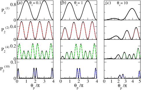
Figure 2: (Color online) Similar results to those in Figure 1 but for a longer repetition period $T=10$ ns.

Next, in Figure 2 we present similar results to those shown in Figure 1 but for a longer laser repetition period of $10$ ns that corresponds to $\gamma T=0.7$. The numerical results for the population of the upper excited state and the analytical results (shown by the solid circles) given by equations (11)-(2.2) and (14)-(15), for $N=1,2,4$, and $10$, are in very good agreement. Of course, compared with a $1$ ns laser repetition period ($\gamma T=0.07$) we expect the upper state population $P_{2}^{(N)}$ to be more damped as the number of pulses in the train increases, and we notice in Figures 2b and 2c that after interaction with $10$ pulses population $P_{2}^{(10)}$ is strongly suppressed and significant Rabi flopping occurs only for a pair of probe and coupling pulses with an effective Rabi frequency area $\theta=2\pi m$, with $m>m_{0}$. This combination of probe and coupling laser pulses is the equivalent of the so called $2\pi$-pulse for a two-level atom that transfers the population from the initial state $|1\rangle$ to the excited state $|2\rangle$ and back again to $|1\rangle$, while for a three-level atom the population is transferred to a superposition of the two lower states $|1\rangle$ and $|3\rangle$, creating a dark state. Actually, the fact that the first peak of the upper state population almost vanished in Figures 2b and 2c at small probe pulse areas, is one of the consequences of the EIT as well as CTP effects, where the population is trapped between the states $|1\rangle$ and $|3\rangle$, while the population of the upper excited state $|2\rangle$ is negligible. In the next subsection we resume and discuss our results for the population dynamics.

In agreement with the theoretical results equations (11)-(15), for weak and moderate coupling pulse areas, $\theta_{c}\leq 1$ in Figures 2a and 2b, the common minima of the populations $P_{2}^{(N)}$ are located around the probe pulse area of $\theta_{p}\simeq 2\pi m$, while for larger coupling pulse area $\theta_{c}=10$, in Figure 2c, the common minima are located around the values of the probe pulse area $\theta_{p}=(2\pi m-\theta_{c}^{2})^{1/2}$, $m>m_{0}$. What we learned for Figures 1 and 2 is that coherent accumulation of excitation decreases for larger coupling pulse areas and is exponentially attenuated by a term which is proportional to the laser repetition period and number of pulses. Depending on the repetition rate the EIT effect occurs for a coupling pulse area larger than some critical value.

3.2 Quantum interference for different probe pulse detunings

Now, it is interesting for spectroscopic investigations to study the upper excited state population as a function of the probe laser detuning for different coupling pulse areas and repetition periods. We show in Figures 3a-3c the population of the excited state $P_{2}^{(N)}$ versus the detuning of the probe laser pulse train. The number of individual pulses of the probe and coupling trains are $N=1,2,4,10$, and $40$, respectively, from top to bottom. The laser parameters are $\Omega_{0p}=0.04$ THz and $\Omega_{0c}=0.1$ THz (Figure 3a), 1 THz (Figure 3b), and 10 THz (Figure 3c). Both laser pulse trains have a Gaussian temporal profile with a duration of each single pulse of $1$ ps and repetition period of 1 ns. For simplicity the coupling laser is considered at resonance, $\delta_{c}=0$. It is clear from Figure 3 that the excited state population changes with the detuning of the probe laser and its periodic structure represent the optical Ramsey fringes Ramsey1950 -Thomas1987 . The resonances occur whenever the probe laser detuning is a multiple of the repetition angular frequency $\omega_{r}$ and the oscillation period of population $P_{2}^{(N)}$ is exactly the period of the frequency spectrum of the laser pulse train [see equation (5)]. The detailed shape of the central Ramsey fringe and the evolution of the resonances with $N$ is presented in detail in Figures 4a-4c for the same parameters as in Figures 3a-3c.

In Figures 5 and 6 are presented similar results as in Figures 3 and 4, but for a longer repetition period of 10 ns. From Figures 3-6 it is clear that the height of the peaks in the population profile increases with the number of pulses in the train $N$, while the width of the population profile becomes narrower as $N$ increases. Depending on the values of the coupling pulse area, we notice three different regimes for the variation of the population $P_{2}^{(N)}$ with probe laser detuning:

• The regime of small coupling pulse area, $\theta_{c}=0.1$, Figures 4a and 6a, where the population of the excited state increases (coherent accumulates) with the number of pulses $N$ for probe laser detunings $\delta_{p}=m\omega_{r}$, where $m$ is an integer. Only after excitation with more than $20$ pulses a small dip appears in the middle of the population profile due to the destructive quantum interference between the two excitation pathways: $|1\rangle$-$|2\rangle$ and $|2\rangle$-$|3\rangle$.

• The regime of moderate coupling pulse area, $\theta_{c}=1$, shown in Figures 4b and 6b, where the EIT effect occurs and the population of the excited state $P_{2}^{(N)}$ exhibits two distinct peaks as $N$ increases, and is negligible at resonance $\delta_{p}=m\omega_{r}$.

• The regime of large coupling pulse area, $\theta_{c}=10$, that is presented in Figures 4c and 6c, where the two peaks of $P_{2}^{(N)}$ are clearly separated by a gap in the frequency domain. This effect is known as the Autler-Townes splitting autler .

The results presented in Figures 4 and 6 show that the coherent accumulation also plays an important role for small and moderate areas of the coupling pulse at off-resonant probe laser detunings. Our results are consistent with the results obtained for a closed $\Lambda$-type system interacting with a femtosecond laser pulse train and a CW laser by an iterative numerical method Soares2010 .

Next, in order to understand the role played by the number of pulses in the trains, populations $P_{k}(t)=|u_{k}(t)|^{2}$, ($k=1,2$, and $3$) and absorption, -Im$[u_{1}(t)u_{2}^{*}(t)]$, are plotted as a function of time for a repetition period of $1$ ns ($\gamma T=0.07$) in Figures 7a-7d, and $10$ ns ($\gamma T=0.7$) in Figures 7e-7h. The probe and coupling laser parameters are $\Omega_{0p}=0.04$ THz and $\Omega_{0c}=0.2$ THz (red solid line), 0.5 THz (green dashed line), and 1 THz (blue dot-dashed line), $\tau=1$ ps, and $\delta_{p}=\delta_{c}=0$. Clearly, Figures 7a-7d and Figures 7e-7h show different dynamics of the populations and absorption for short and large repetition period. For small coupling pulse area $\theta_{c}=0.2$ and $T=1$ ns, in Figure 7b, the population $P_{2}$ increases with time (the excitation accumulates since there is less time for atom to relax between two consecutive pulses), it reaches a maximum value for $t\simeq 13T$, and after that it decreases to negligible values. The absorption (Figure 7d) does not take negligible values and there is a small population transfer from state $|1\rangle$ to state $|3\rangle$. For larger coupling pulse areas $\theta_{c}=0.5$ and $1$ the population $P_{2}$ oscillates sinusoidally in time. For a longer repetition period $T=10$ ns (Figures 7e-7h) both population $P_{2}$ (Figure 7f) and absorption (Figure 7h) accumulate very fast during the first few pulses and then start to decrease. In comparison with the repetition period of $1$ ns population $P_{2}$ and absorption present a strong oscillatory behavior from one pulse to the next one in the train, a sawtooth profile that describes successive excitations of the upper level followed by its spontaneous decay Felinto2004 . For larger coupling pulse areas $\theta_{c}=0.5$ and $1$, after the EIT and AT regime occur for $t$ larger than $30T$ and $10T$, respectively, the populations $P_{1}$ and $P_{3}$ reach stationary values that do not change with the number of pulses $N$, while the excited state population $P_{2}$ and absorption are negligible (in Figures 7e-7h). This temporal dynamics explains the evolution of the EIT and AT resonance of $P_{2}$ in Figures 3-6. The analytical results calculated at the end of each pulse given by equation (15) (indicated by solid circles in Figures 7b and 7f), are in good agreement with the numerical results.

4 Summary

In this paper we have studied the quantum interference between the excitation pathways in a three-level $\Lambda$-type atom interacting with short probe and coupling laser pulse trains, beyond the steady state approximation, under EIT conditions. We have investigated the modification induced by the laser pulse trains in a lambda-type atom in terms of upper excited state population for different pulse areas and different detunings. We have numerically integrated the probability amplitude equations that describe the interaction of the $\Lambda$-type atom with the two laser pulse trains. For resonant laser pulse trains with a rectangular temporal profile we have derived analytical formulas for the population of the upper excited state at the end of the pulse. For the atomic and laser parameters used in the present paper we obtain a very good agreement between the analytical results (calculated for rectangular pulse envelopes) and the numerical results (calculated for Gaussian pulse envelopes with identical pulse areas as for rectangular shape). We have discussed the dynamics of the upper state population and presented numerical and analytical results for small, moderate, and large coupling pulse areas for resonant probe and coupling laser trains. We have showed that we can control the interaction of a $\Lambda$-type atom with two laser pulse trains under the EIT conditions, for small probe pulse area while the area of the coupling pulse is moderate, by manipulating certain parameters of the lasers such that: Rabi frequencies, pulse repetition period, number of individual pulses, and detunings.

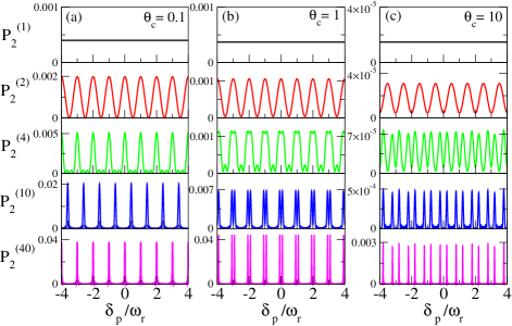
Figure 3: (Color online) Population of the upper excited state $P_{2}^{(N)}$ as a function of the probe laser detuning. The number of individual pulses in the trains are $N=1,2,4,10,$ and $40$ (from top to bottom). The probe laser area is $\theta_{p}=0.04$ and the coupling laser area $\theta_{c}$ is $0.1$ in (a), 1 in (b) and 10 in (c), from top to bottom. Both laser pulse trains have a Gaussian temporal envelope with the duration $\tau=1$ ps, the repetition period $T=1$ ns, and the coupling laser detuning is $\delta_{c}=0$.

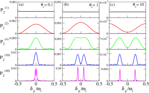
Figure 4: (Color online) The same results as those in Figure 3, but detailed for a small detuning range around $-\omega_{r}/2\leq\delta_{p}\leq\omega_{r}/2$, representing the central Ramsey fringe.

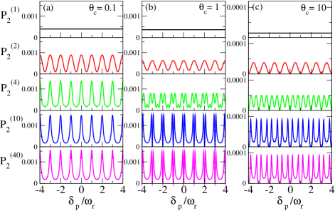
Figure 5: (Color online) Similar results to those in Figure 3 but for a repetition period $T=10$ ns.

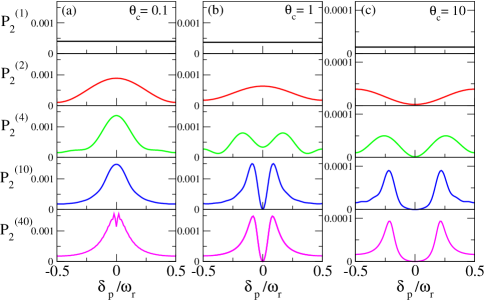
Figure 6: (Color online) The same results as those in Figure 5, but detailed for a small detuning range around $-\omega_{r}/2\leq\delta_{p}\leq\omega_{r}/2$, representing the central Ramsey fringe.

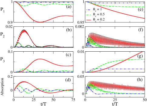
Figure 7: (Color online) Populations $P_{1}$, $P_{2}$, and $P_{3}$ and absorption as a function of time for a repetition period of $1$ ns in (a)-(d) and $10$ ns in (e)-(h). The probe laser area is $\theta_{p}=0.04$ and the coupling laser area is $\theta_{c}=0.2$ (red solid line), $0.5$ (green dashed line), and $1$ (blue dot-dashed line). The solid circles in (b) and (f) represents the analytical results calculated at the end of each pulse. Both laser pulse trains have a Gaussian temporal envelope with the duration $\tau=1$ ps and detunings $\delta_{p}=\delta_{c}=0$.

- (1) M. Shapiro and P. Brumer, in Advances in Atomic, Molecular and Optical Physics, edited by B. Bederson and H. Walther (Academic Press, San Diego, 1999), Vol. 42, pp. 287-345
- (2) F. Ehlotzky, Phys. Rep. 345, 175 (2001)
- (3) S. E. Harris, Phys. Today 50, 36 (1997)
- (4) J. P. Marangos, J. Mod. Optics 45, 471 (1998)
- (5) K. Bergmann, H. Theuer, and B. W. Shore, Rev. Mod. Phys. 70 1003 (1998)
- (6) O. Kocharovskaya and Ya. I. Khanin, Sov. Phys. JETP 63, 945 (1986)
- (7) K. J. Boller, A. Imamoglu, and S. E. Harris, Phys. Rev. Lett. 66, 2593 (1991)
- (8) M. Fleischhauer, A. Imamoglu, and J. P. Marangos, Rev. Mod. Phys. 77, 633 (2005)
- (9) G. Alzetta, A. Gozzini, L. Moi, and G. Oriolis, Nuovo Cimento B 36, 5 (1976)
- (10) A. Marian, M. C. Stowe, J. R. Lawall, D. Felinto, and J. Ye, Science 306, 2063 (2004)
- (11) M. C. Stowe, F. C. Cruz, A. Marian, and J. Ye, Phys. Rev. Lett. 96, 153001 (2006)
- (12) D. Felinto, C. A. C. Bosco, L. H. Acioli, and S. S. Vianna, Opt. Commun. 215, 69 (2003)
- (13) D. Felinto, L. H. Acioli, and S. S. Vianna, Phys. Rev. A 70, 043403 (2004)
- (14) S. Zhdanovich, E. A. Shapiro, M. Shapiro, J. W. Hepburn, and V. Milner, Phys. Rev. Lett. 100, 103004 (2008)
- (15) H. Tang and T. Nakajima, Opt. Commun. 281, 4671 (2008)
- (16) A. A. Soares and L. E. E. de Araujo, J. Phys. B: At. Mol. Opt. Phys. 43, 085003 (2010)
- (17) M. P. Moreno and S. S. Vianna, J. Opt. Soc. Am. B 28, 1124 (2011)
- (18) E. Ilinova and A. Derevianko, Phys. Rev. A 86, 013423 (2012)
- (19) B. W. Shore, Acta Physica Slovaca 58, 243 (2008)
- (20) N. Vitanov and P. L. Knight, Phys. Rev. A 52, 2245 (1995)
- (21) D. Aumiler, T. Ban, and G. Pichler, Phys. Rev. A 79, 063403 (2009)
- (22) D. Felinto, C. A. C. Bosco, L. H. Acioli, and S. S. Vianna, Phys. Rev. A 64, 063413 (2001)
- (23) L. Allen and J.H. Eberly, Optical resonance and two-level atoms (Wiley, New York 1975)
- (24) N. F. Ramsey, Phys. Rev. 78, 695 (1950)
- (25) G. F. Thomas, Phys. Rev. A 35, 5060 (1987)
- (26) S. H. Autler and C. H. Townes, Phys. Rev. 100, 703 (1955)