Symmetries in elastic scattering of electrons by hydrogen atoms in a two-color bicircular laser field

Abstract

We consider the elastic scattering of electrons by hydrogen atoms in the presence of a two-color circularly polarized laser field in the domain of moderate intensities below $10^{13}$ W/cm² and high projectile energies. A hybrid approach is used, where for the interaction of the incident and scattered electrons with the laser field we employ the Gordon-Volkov wave functions, while the interaction of the hydrogen atom with the laser field is treated in second-order perturbation theory. Within this formalism, a closed analytical solution is derived for the nonlinear differential cross section, which is valid for circular as well linear polarizations. Simple analytical expressions of differential cross section are derived in the weak field domain for two-color laser field that is a combination of the fundamental and its second or third harmonics. It is shown that the nonlinear differential cross sections depend on the dynamical phase of the scattering process and on the helicities of the two-color circularly polarized laser field. A comparison between the two-photon absorption scattering signal for two-color co- and counter-rotating circularly polarized laser fields is made for even ($2\omega$) or odd ($3\omega$) harmonics, and the effect of the intensity ratio of the two-color laser field components is studied. We analyze the origin of the symmetries in the differential cross sections and we show that the modification of the photon helicity implies a change in the symmetries of the scattering signal.

I INTRODUCTION

The study of laser-assisted and laser-induced atomic processes has attracted an increasing theoretical as well experimental interest in the last 30 years. In particular, such interest is justified because of the possibility of controlling the atomic processes by using two-color (or multicolor) fields and manipulating the laser parameters such as relative phase and intensities ratio between the monochromatic components of the fields, polarizations, etc. ehl2001 . The physical mechanism for controlling laser-assisted and laser-induced atomic processes using two-color fields resides in the different pathways, due to monochromatic components of the field, leading to the same final state of the atomic system involving different numbers of exchanged (absorbed and/or emitted) photons. Thus, the quantum-mechanical interference occurring among different transition amplitudes, which contribute to the same final state but through distinct pathways, offers the possibility of controlling laser-assisted and laser-induced atomic processes. Different kinds of electronic transitions were investigated, such as laser-assisted elastic and inelastic electron-atom scattering in a laser field (free-free transitions), laser-induced excitation of atoms (bound-bound transitions), or laser-induced ionization of atoms (bound-free transitions). It is well known that laser-assisted electron-atom scattering is a subject of particular interest in applied domains such as laser and plasma physics plasma , astrophysics astro , or fundamental atomic collision theory massey . Detailed reports on the laser-assisted electron-atom collisions can be found in several review papers mason ; ehl1998 and books bransden ; joa2012 . Recently, the study of electron-atom scattering in the presence of a laser field has attracted considerable attention musa ; Harak ; Kanya ; Kanya2 ; gabi2017 , especially because of the progress of experimental techniques.

A two-color bicircular electromagnetic field represents a superposition of two circularly polarized (CP) fields which rotate in the same plane, with different photon energies and the same helicities (corotating CP fields) or opposite helicities (counter-rotating CP fields). More than 20 years ago, it was suggested that CP high-order harmonics can be generated by counter-rotating bicircular fields for a zero-range-potential model atom Long and it was experimentally shown that the emission of these harmonics is very efficient compared to corotating CP and linearly polarized (LP) fields Eichmann . The recent experimental confirmation that the generated high harmonics are circularly polarized Fleischer2014 , allowing the direct generation of CP soft x-ray pulses, has generated an increasing interest in studying different laser-induced processes by co- and counter-rotating CP laser fields such as strong-field ionization Mancuso15 , nonsequential double ionization Mancuso16 , or laser-assisted electron-ion recombination Odzak1 ; Odzak .

In the present paper, we study the elastic scattering of fast electrons by hydrogen atoms in their ground state in the presence of two-color bicircular laser fields. Obviously, the physical mechanism occurring in laser-assisted processes for two-color fields is the interference among different photon pathways leading to the same final state, and by using CP fields another parameter (the dynamical phase of the scattering process) plays an important role. Theoretical studies involving monochromatic CP fields with the atomic dressing taken into account in second-order of time-dependent perturbation theory (TDPT) were performed for laser-assisted electron-hydrogen scattering by Cionga and coworkers acgabi2 ; acgabiopt . In contrast to these past studies, we investigate here a different regime of a bichromatic CP field where the monochromatic components of the field rotate in the same plane and in the same or opposite directions. To our knowledge, there are no other theoretical studies regarding elastic laser-assisted electron-atom scattering processes in a two-color bicircular laser field which include the atomic dressing in second-order TDPT. The paper is structured as follows. In Sec. II we present the semiperturbative method used to obtain the analytical formulas for the differential cross section (DCS) for a two-color CP laser field with different polarizations. Because the scattering process under investigation is a very complex problem, the theoretical approach poses considerable difficulties and few assumptions are made. Moderate field intensities below $10^{13}$ W/cm² and fast projectile electrons are considered in order to safely neglect the second-order Born approximation in the scattering potential as well as the exchange scattering b-j . The interaction between the projectile electrons and the laser field is described by Gordon-Volkov wave functions volkov , whereas the interaction of the hydrogen atom with the laser field is described within the second-order TDPT in the field vf1 . The derived analytical formula for the DCS, which includes the second-order atomic dressing effects, is valid for two-color fields with circular and/or linear polarizations. In Sec. III, we provide simple analytic formulas in a closed form for DCSs in the laser-assisted elastic scattering in the weak field limit, for the superposition of the fundamental laser field with its second or third harmonic, which exhibit an explicit dependence on the field polarizations. The numerical results are discussed in Sec. IV, where the DCSs by corotating and counter-rotating CP fields are compared and analyzed as a function of the scattering and azimuthal angles of the projectile electron at different intensity ratios of the monochromatic components of the bicircular laser field. Atomic units (a.u.) are used throughout this paper unless otherwise specified.

II Semiperturbative theory at moderate laser intensities for a two-color bicircular laser field

The laser-assisted scattering of electrons by hydrogen atoms in a two-color laser field is formally represented as

$$e^{-}(E_{p},\mathbf{p})+{\rm H}(1s)+N_{1i}\,\gamma\,(\omega_{1},\bm{\varepsilon}_{1})+N_{mi}\,\gamma\,(\omega_{m},\bm{\varepsilon}_{m})\to$$

$$e^{-}(E_{p^{\prime}},{\mathbf{p^{\prime}}})+{\rm H}(1s)+N_{1f}\,\gamma\,(\omega_{1},\bm{\varepsilon}_{1})+N_{mf}\,\gamma\,(\omega_{m},\bm{\varepsilon}_{m}),$$ (1)

where $E_{p}\,(E_{p^{\prime}})$ and $\mathbf{p}\,(\mathbf{p^{\prime}}$) denote the kinetic energy and the momentum vector of the incident (scattered) projectile electron. $\gamma\,(\omega_{k},\bm{\varepsilon}_{k})$ represents a photon with the energy $\omega_{k}$ and the unit polarization vector $\bm{\varepsilon}_{k}$, and $N_{k}=N_{ki}-N_{kf}$ denotes the net number of exchanged photons between the projectile-atom system and each monochromatic component of the two-color laser field, with $k=1$ and $m$. The two-color laser field is treated classically and is considered as a superposition of two coplanar CP electric fields,

$${\bf E}(t)=\frac{i}{2}[{E}_{01}\bm{\varepsilon}_{1}\exp(-i\omega_{1}t)+{E}_{0m}\bm{\varepsilon}_{m}\exp(-i\omega_{m}t)]+\rm{c.c.},$$ (2)

where ${E}_{0k}$ represents the peak amplitude of the monochromatic components of electric field and $\rm{c.c.}$ denotes the complex conjugate of the right-hand-side term. For a bicircular field the polarization vector of the first laser beam is defined as $\bm{\varepsilon}_{1}=\bm{\varepsilon}_{+}=(\mathbf{e}_{j}+i\mathbf{e}_{l})/\sqrt{2}$, where $\mathbf{e}_{j}$ and $\mathbf{e}_{l}$ are the unit vectors along two orthogonal directions, and the second laser beam has the same polarization $\bm{\varepsilon_{m}}=\bm{\varepsilon}_{+}$ (the so-called corotating polarization), or is circularly polarized in the opposite direction $\bm{\varepsilon_{m}}=\bm{\varepsilon}_{-}=(\textbf{e}_{j}-i\textbf{e}_{l})/\sqrt{2}$ (the so-called counter-rotating polarization). Thus, the two-color bicircular electric field vector can be easily calculated as

$${\bf E}(t)=\mathbf{e}_{j}\left({E}_{01}\sin\omega_{1}t+{E}_{0m}\sin\omega_{m}t\right)/\sqrt{2}-\mathbf{e}_{l}\left({E}_{01}\cos\omega_{1}t+\eta\,{E}_{0m}\cos\omega_{m}t\right)/\sqrt{2},$$ (3)

where the helicity takes the values $\eta=+1$ for corotating CP fields and $\eta=-1$ for counter-rotating CP fields.

II.1 Projectile electron and atomic wave functions

We consider moderate laser intensities and fast projectiles, which imply that the strength of the laser field is lower than the Coulomb field strength experienced by an electron in the first Bohr orbit of the hydrogen atom and the energy of the projectile electron is much higher than the energy of the bound electron in the first Bohr orbit ehl1998 . The interaction between the projectile electron and the two-color laser field is treated by a Gordon-Volkov wave function volkov , and the initial and final states of the projectile electron are given by

$$\chi_{\mathbf{p}}({\mathbf{R}},t)={(2\pi)^{-3/2}}\exp\left[-iE_{p}t+i{\mathbf{p}}\cdot{\mathbf{R}}-i{\mathbf{p}}\cdot\bm{\alpha}_{1}(t)-i{\mathbf{p}}\cdot\bm{\alpha}_{m}(t)\ \right],$$ (4)

where $\mathbf{R}$ denotes the position vector and $\bm{\alpha}_{k}(t)$, with $k=1$ and $m$, describes the classical oscillation motion of the projectile electron in the bicircular electric fields defined by Eq. (3),

$$\bm{\alpha}_{1}(t) = \alpha_{01}\left(\mathbf{e}_{j}\sin\omega_{1}t+\mathbf{e}_{l}\cos\omega_{1}t\right)/\sqrt{2},$$ (5)

$$\bm{\alpha}_{m}(t) = \alpha_{0m}\left(\mathbf{e}_{j}\sin\omega_{m}t+\eta\,\mathbf{e}_{l}\cos\omega_{m}t\right)/\sqrt{2},$$ (6)

where ${\alpha_{0k}}=\sqrt{{I}_{k}}/\omega_{k}^{2}$ is the peak amplitude and ${I}_{k}={E}_{0k}^{2}$ is the peak laser intensity. In Eq. (4) the terms which are proportional to the ponderomotive energy $U_{p,k}={I}_{k}/4\omega_{k}^{2}$ are neglected since the calculations presented in this paper are made at moderate field intensities below $10^{13}$ W/cm². For example, at a field intensity of $10^{12}$ W/cm² and a photon energy of $1.55$ eV, the ponderomotive energy is about $0.06$ eV and therefore is negligible in comparison with the photon and projectile energies.

At moderate field strengths the interaction of the hydrogen atom with the two-color laser field is considered within the second-order TDPT and an approximate solution for the wave function in the second-order TDPT for an electron bound to a Coulomb potential in the presence of an electric field, Eq. (2), is written as

$$\Psi_{1s}\left(\mathbf{r},t\right)=\exp{(-i{E}_{1s}t)}\left[\psi_{1s}(\mathbf{r},t)+\psi_{1s}^{(1)}(\mathbf{r},t)+\psi_{1s}^{(2)}(\mathbf{r},t)\right]\,,$$ (7)

where $\bm{r}$ represents the position vector of the bound electron, ${E}_{1s}$ is the energy of the ground state, $\psi_{1s}$ is the unperturbed wave function of the ground state, and $\psi_{1s}^{(1)}$ and $\psi_{1s}^{(2)}$ represent the first- and second-order radiative corrections to the atomic wave function. We employ the following expression of the first-order correction,

$$\psi_{1s}^{(1)}(\mathbf{r},t)=-\sum_{k=1,m}\frac{\alpha_{0k}\omega_{k}}{2}\left[\bm{\varepsilon}_{k}\cdot\mathbf{w}_{100}(\Omega^{+}_{k};\mathbf{r})\exp{(-i\omega_{k}t)}+\bm{\varepsilon}_{k}^{*}\cdot\mathbf{w}_{100}(\Omega^{-}_{k};\mathbf{r})\exp{(i\omega_{k}t)}\right],$$ (8)

where ${\bf{w}}_{100}$ is the linear-response vector vf1 , which depends on the energies $\Omega_{k}^{\pm}={E}_{1s}\pm\omega_{k}$, that is expressed as

$${\bf{w}}_{100}(\Omega;\mathbf{r})=i(4\pi)^{-1/2}{\cal B}_{101}(\Omega;r)\,\hat{\mathbf{r}}.$$ (9)

The radial function ${\cal B}_{101}$ is calculated using the Coulomb Green’s function including both bound and continuum eigenstates vf1 and $\hat{\mathbf{r}}=\mathbf{r}/|\mathbf{r}|$. The second-order correction to the atomic wave function $\psi_{1s}^{(2)}$ is written in terms of the quadratic response tensors vf2 as,

$${w}_{jl,100}(\Omega^{\prime},\Omega;\mathbf{r})=\frac{1}{6\sqrt{\pi}}\left\{\frac{3x_{j}x_{l}}{r^{2}}{\cal B}_{10}^{21}(\Omega^{\prime},\Omega;\mathbf{r})+\delta_{jl}[{\cal B}_{10}^{01}(\Omega^{\prime},\Omega;\mathbf{r})-{\cal B}_{10}^{21}(\Omega^{\prime},\Omega;\mathbf{r})]\right\},$$ (10)

and

$$\widetilde{w}_{jl,\rm 100}({E_{1s}},\Omega;\mathbf{r})=\frac{1}{2}\lim_{\epsilon\to 0}\left[w_{jl,\rm 100}({E_{1s}+\epsilon},\Omega;\mathbf{r})+w_{jl,\rm 100}({E_{1s}-\epsilon},\Omega;\mathbf{r})\right],$$ (11)

where the radial functions ${\cal B}_{10}^{01}$ and ${\cal B}_{10}^{21}$ are calculated in Ref. vf2 , with $j$ and $l=1,2,3$. The explicit form of the second-order radiative correction $\psi_{1s}^{(2)}$ for a two-color laser field is given in Appendix A.

II.2 Scattering matrix

To proceed, once we have obtained the atomic and projectile electron wave function in the laser field we are able to derive the scattering matrix for the electron-atom scattering in the static potential $V(r,R)=-1/R+1/{|\bf{R}-\bf{r}|}.$ We assume fast projectile electrons such that the scattering process can be well treated within the first-order Born approximation in the scattering potential $V(r,R)$ and we use a semiperturbative treatment for the scattering process similar to the one developed by Byron and Joachain b-j . The scattering matrix element is calculated at high projectile energies, $E_{p}>100$ eV, where the exchange effects can be safely neglected, as

$$S_{fi}=-i\int_{-\infty}^{+\infty}dt\langle\chi_{\mathbf{p^{\prime}}}(\mathbf{R},t)\Psi_{1s}(\mathbf{r},t)|V(r,R)|{\chi}_{\mathbf{p}}(\mathbf{R},t)\Psi_{1s}(\mathbf{r},t)\rangle\,,$$ (12)

where $\chi_{\mathbf{p}_{i}}$ and $\chi_{\mathbf{p^{\prime}}}$ are the initial and final Gordon-Volkov wave functions of the projectile electron in the two-color laser field and $\Psi_{1s}$ represents the wave function of the bound electron in the laser field, given by Eqs. (4) and (7), respectively.

For commensurate photon energies, $\omega_{m}=m\omega_{1}$, the energies of the projectile electron satisfy the conservation relation $E_{p^{\prime}}-E_{p}=N\omega_{1}$, with $N\omega_{1}\equiv N_{1}\omega_{1}+N_{m}\omega_{m}$. Using the Jacobi-Anger expansion formula $\exp{(ia\sin\omega t)}=\sum_{N}J_{N}(a)\exp{(iN\omega t)},$ we develop the field dependent part of the Gordon-Volkov wave functions in the scattering matrix, Eq. (12), in terms of the phase-dependent generalized Bessel functions, $B_{N}$, Watson ; varro , as

$$\exp{[-i\bm{\alpha}_{1}(t)\cdot\mathbf{q}-i\bm{\alpha}_{m}(t)\cdot\mathbf{q}]}=\sum_{N=-\infty}^{+\infty}B_{N}(R_{1},R_{m};\phi_{1},\phi_{m})\exp{(-iN\omega_{1}t+iN\phi_{1})},$$ (13)

where

$$B_{N}(R_{1},R_{m};\phi_{1},\phi_{m})=\sum_{l=-\infty}^{+\infty}J_{N-ml}(R_{1})J_{l}(R_{m})\exp{[-il(m\phi_{1}-\phi_{m})]}.$$ (14)

Here $\mathbf{q}$ denotes the momentum transfer vector of the projectile electron, i.e., $\mathbf{q}=\mathbf{p}-\mathbf{p^{\prime}}$, and the arguments of the generalized Bessel function are $R_{k}=\alpha_{0k}|\bm{\varepsilon}_{k}\cdot\mathbf{q}|$ and $\phi_{k}$, where the dynamical phase is defined as $e^{i\phi_{k}}=(\bm{\varepsilon}_{k}\cdot\mathbf{q})/|\bm{\varepsilon}_{k}\cdot\mathbf{q}|$, with $k=1$ and $m$. Specifically, for a CP field we obtain $R_{k}=\alpha_{0k}\sqrt{(\mathbf{e}_{j}\cdot\mathbf{q})^{2}+(\mathbf{e}_{l}\cdot\mathbf{q})^{2}}/\sqrt{2}$ and $\phi_{k}=\arctan{(\mathbf{e}_{l}\cdot\mathbf{q})/(\mathbf{e}_{j}\cdot\mathbf{q})}+s\pi$, where $s$ is an integer. Obviously, a change of helicity of the CP field, i.e., $\bm{\varepsilon}\to\bm{\varepsilon}^{*}$, leads to a change of the sign of the dynamical phase, $\phi_{k}\to-\phi_{k}$. In contrast, for a LP field the arguments of the $B_{N}$ function are simply given by $R_{k}^{LP}=\alpha_{0k}|\mathbf{e}_{j}\cdot\mathbf{q}|$ and $\phi_{k}^{LP}=s\pi$.

By substituting Eqs. (4),(7) and (13) into Eq. (12) we obtain, after integrating over time and projectile electron coordinate, the scattering matrix $S_{fi}$ for elastic electron-hydrogen collisions in a two-color laser field,

$$S_{fi}=-2\pi i\sum_{N=-\infty}^{+\infty}T_{fi}(N)\,\delta(E_{p^{\prime}}-E_{p}-N\omega_{1})\,,$$ (15)

where the Dirac $\delta$ function assures the energy conservation, and $T_{fi}(N)$ represents the total transition amplitude for the elastic scattering process, which can be written as the sum of three terms

$$T_{fi}(N)=T^{(0)}(N)+T^{(1)}(N)+T^{(2)}(N).$$ (16)

Finally, the nonlinear DCS for the scattering of the projectile in the solid angle $\Omega$ with the energy of the projectile modified by $N\omega_{1}$, reads

$$\frac{d{\sigma}(N)}{d\Omega}={(2\pi)}^{4}\frac{{p^{\prime}}{(N)}}{p}{|T^{(0)}(N)+T^{(1)}(N)+T^{(2)}(N)|}^{2},$$ (17)

in which the final momentum of the projectile is calculated as ${p^{\prime}}(N)={(p^{2}+2N\omega_{1})}^{1/2}$. The derivation of the transition amplitudes $T^{(i)}(N)$, ($i=0,1,2$) is briefly described in the next subsections.

II.2.1 Electronic transition matrix elements

The first term, $T^{(0)}$, on the right-hand side of Eq. (16) represents the elastic transition amplitude due to projectile electron contribution in which the atomic dressing is neglected,

$$T^{(0)}(N)=B_{N}(R_{1},R_{m};\phi_{1},\phi_{m})\langle\psi_{1s}|F(\mathbf{q},\mathbf{r})|\psi_{1s}\rangle,$$ (18)

where the form factor is given by $F(\mathbf{q},\mathbf{r})=\left[\exp{(i\mathbf{q}\cdot\mathbf{r})}-1\right]/{(2\pi^{2}q^{2})}$. By substituting the partial-wave expansion of the exponential term $\exp{(i\mathbf{q}\cdot\mathbf{r})}$ in the form factor and performing the angular integration, the electronic transition amplitude $T^{(0)}$ reads

$$T^{(0)}(N)=-\frac{1}{(2\pi)^{2}}f_{el}^{B_{1}}(q)\,B_{N}(R_{1},R_{m};\phi_{1},\phi_{m}),$$ (19)

where the term $f_{el}^{B_{1}}(q)={2(q^{2}+8)}/{(q^{2}+4)^{2}}$ represents the first-order Born approximation of the scattering amplitude for field-free elastic scattering process, and the laser field dependence is contained in the arguments of the generalized Bessel function only. If the atomic dressing is negligible in Eq. (17), the DCS for $N$-photon exchange is approximated as

$$\frac{d{\sigma}(N)}{d\Omega}\simeq\frac{4p^{\prime}}{p}\frac{(q^{2}+8)^{2}}{(q^{2}+4)^{4}}\left|B_{N}(R_{1},R_{m};\phi_{1},\phi_{m})\right|^{2},$$ (20)

which is the equivalent of the Bunkin and Fedorov formula bf , for fast electron scattering on hydrogen atoms in a two-color CP laser field, in which the laser-atom interaction is neglected.

II.2.2 First-order atomic transition matrix elements

The second term, $T^{(1)}$, on the right-hand side of the transition amplitude, Eq. (16), represents the first-order atomic transition amplitude and it occurs due to alteration of the atomic state by the two-color laser field, which is described by the first-order radiative correction $\psi^{(1)}(\mathbf{r},t)$. Obviously, only one photon is emitted or absorbed between the two-color laser field and the bound electron. After some algebra, the atomic transition amplitude $T^{(1)}$ is expressed as

$$T^{(1)}(N)=-\sum_{k=1,m}\frac{\alpha_{0k}\omega_{k}}{2}\left[B_{N-k}\;{\cal M}_{at}^{(1)}(\omega_{k},\mathbf{q})e^{-ik\phi_{1}}+B_{N+k}\;{\cal M}_{at}^{(1)}(-\omega_{k},\mathbf{q})e^{ik\phi_{1}}\right],$$ (21)

where ${\cal M}_{at}^{(1)}(\omega_{k},\mathbf{q})$ denotes a specific first-order atomic transition matrix element related to one-photon absorption

$${\cal M}_{at}^{(1)}(\omega_{k},\mathbf{q})=\sum_{j=1}^{3}{\varepsilon}_{kj}[\langle\psi_{1s}|F(\mathbf{q})|{{w}}_{j,100}(\Omega_{k}^{+})\rangle+\langle{w}_{j,100}(\Omega_{k}^{-})|F(\mathbf{q})|\psi_{1s}\rangle],$$ (22)

whereas the transition matrix element ${\cal M}_{at}^{(1)}(-\omega_{k},\mathbf{q})$ is related to one-photon emission and is obtained from ${\cal M}_{at}^{(1)}(\omega_{k},\mathbf{q})$ with the replacements $\omega_{k}\to-\omega_{k}$ (i.e., $\Omega_{k}^{\pm}\to\Omega_{k}^{\mp}$) and $\bm{\varepsilon}_{k}\to\bm{\varepsilon}_{k}^{*}$. The first term on the right-hand side of Eq. (22) describes first the atom interacting with the laser field followed by the projectile electron-atom interaction, while in the second term the projectile electron-atom interaction precedes the atom-laser interaction. For the sake of simplicity, the arguments of the generalized Bessel functions $B_{N}(R_{1},R_{m};\phi_{1},\phi_{m})$ are now dropped off in Eq. (21) and throughout this paper. By using the partial-wave expansion of the exponential term $\exp{(i\mathbf{q}\cdot\mathbf{r})}$ and the definition of ${\mathbf{w}}_{100}$ given by Eq. (9), after performing the angular integration, we obtain for the atomic transition matrix element, Eq. (22),

$${\cal M}_{at}^{(1)}(\omega_{k},\mathbf{q})=-\frac{\bm{\varepsilon}_{k}\cdot\hat{\mathbf{q}}}{2{\pi}^{2}q^{2}}\left[{\cal J}_{101}^{a}(\Omega_{k}^{+},q)-{\cal J}_{101}^{a}(\Omega_{k}^{-},q)\right],$$ (23)

in which ${\cal J}_{101}^{a}$ is an atomic radial integral defined as

$${\cal J}_{101}^{a}(\Omega_{k},q)={\int}_{0}^{+\infty}dr\ r^{2}R_{10}(r)j_{1}(qr){\cal B}_{101}(\Omega_{k};r),$$ (24)

where $j_{1}(qr)$ represents the spherical Bessel function of first kind and $\hat{\mathbf{q}}=\mathbf{q}/|\mathbf{q}|$. An analytic expression of ${\cal J}_{101}^{a}$ in terms of hypergeometric functions is given by Eq. (36) of Ref. acgabi2 . Finally, the atomic transition amplitude, $T^{(1)}$, is obtained by substituting Eq. (22) into Eq. (21)

$$T^{(1)}(N) = \sum_{k=1,m}\frac{\alpha_{0k}\omega_{k}}{4{\pi}^{2}q^{2}}\left[(\bm{\varepsilon}_{k}\cdot\hat{\mathbf{q}})B_{N-k}{\cal J}_{101}(\omega_{k},q)e^{-ik\phi_{1}}\right.$$ (25)

$$\left.-(\bm{\varepsilon}_{k}^{*}\cdot\hat{\mathbf{q}})B_{N+k}{\cal J}_{101}(\omega_{k},q)e^{ik\phi_{1}}\right],$$

where the radial integral ${\cal J}_{101}$ is calculated as the difference between two atomic radial integrals given by Eq. (24), ${\cal J}_{101}(\omega_{k},q)={\cal J}_{101}^{a}(\Omega_{k}^{+},q)-{\cal J}_{101}^{a}(\Omega_{k}^{-},q)$.

In addition, in the low-photon energy limit ($\omega\ll E_{n}-E_{1s}$), the atomic radial integral can be approximated as ${\cal J}_{101}(\omega,q)\simeq\omega\,q\,\alpha_{d}(q)$, where $\alpha_{d}$ represents the dynamic dipole polarizability due to polarization of the target by the projectile electron milo ; acgabi2 ; acgabi3 . The analytical form of the dynamic dipole polarizability within the first-order TDPT acgabi2 in low-photon energy limit is calculated as

$$\alpha_{d}(q,Z)=\frac{\alpha_{s}(Z)}{{3[1+q^{2}/(2Z)^{2}]}^{3}}\left[1+\frac{2}{1+q^{2}/(2Z)^{2}}\right]\;,$$ (26)

where $\alpha_{s}(Z)=4.5\,Z^{-4}$ denotes the static dipole polarizability of a H-like ion in the ground state bransden . We point out that Eq. (26) describes the target dressing effects at both small and large scattering angles in contrast to the dynamic dipole polarizability calculated in Ref. milo for the hydrogen atom, $\alpha_{d}(q)=\alpha_{s}/{(1+q^{2}/4)}^{3}$, which gives accurate results only at small scattering angles.

II.2.3 Second-order atomic transition matrix elements

The third term, $T^{(2)}$, on the right-hand side of the transition amplitude, Eq. (16), represents the second-order atomic transition amplitude and occurs due to modification of the atomic state by the laser field, described by the second-order radiative correction $\psi^{(2)}(\mathbf{r},t)$, which is given in Appendix A. In this approach only two photons are exchanged (absorbed, emitted, or absorbed and emitted) between the two-color CP laser field and the bound electron. After some calculation the atomic transition amplitude $T^{(2)}$ reads

$$T^{(2)}(N) = \sum_{k=1,m}\frac{\alpha_{0k}^{2}\omega_{k}^{2}}{4}\left\{B_{N-2k}{\cal M}_{at}^{(2)}(\omega_{k},\mathbf{q})e^{-2ik\phi_{1}}\right.$$ (27)

$$+B_{N+2k}{\cal M}_{at}^{(2)}(-\omega_{k},\mathbf{q})e^{2ik\phi_{1}}$$

$$\left.+B_{N}\left[\widetilde{\cal M}_{at}^{(2)}({E}_{1s},\omega_{k})+\widetilde{\cal M}_{at}^{(2)}({E}_{1s},-\omega_{k})\right]\right\}$$

$$+\frac{\alpha_{01}\alpha_{0m}\omega_{1}\omega_{m}}{4}\left[B_{N-m-1}{\cal N}_{at}^{(2)}(\omega_{1},\omega_{m},\mathbf{q})e^{-i(m+1)\phi_{1}}\right.$$

$$+B_{N+m+1}{\cal N}_{at}^{(2)}(-\omega_{1},-\omega_{m},\mathbf{q})e^{i(m+1)\phi_{1}}$$

$$+B_{N-m+1}{\cal N}_{at}^{(2)}(-\omega_{1},\omega_{m},\mathbf{q})e^{-i(m-1)\phi_{1}}$$

$$\left.+B_{N+m-1}{\cal N}_{at}^{(2)}(\omega_{1},-\omega_{m},\mathbf{q})e^{i(m-1)\phi_{1}}\right].$$

We point out that the explicit or implicit presence of the dynamical phase factors $e^{i\phi_{1}}$ and $e^{i\phi_{m}}$ in the electronic and atomic transitions amplitudes, Eqs. (19), (25) and (27), can give different interference terms in DCS for corotating in comparison to counter-rotating CP field. Specific second-order atomic transition matrix elements related to two-photon exchange appear in Eq. (27). Thus, ${\cal M}_{at}^{(2)}$ is related to absorption of two identical photons of energy $\omega_{k}$ and complex polarization $\bm{\varepsilon}_{k}$,

$${\cal M}_{at}^{(2)}(\omega_{k},\mathbf{q}) = \sum_{j,l=1}^{3}\varepsilon_{kj}\varepsilon_{kl}\left[\langle w_{j,100}(\Omega_{k}^{-})|F(\mathbf{q})|{w}_{l,100}(\Omega_{k}^{+})\rangle\right.$$ (28)

$$\left.+\langle\psi_{1s}|F(\mathbf{q})|w_{jl,100}(\Omega_{k}^{\prime\,+},\Omega_{k}^{+})\rangle+\langle w_{jl,100}(\Omega_{k}^{\prime\,-},\Omega_{k}^{-})|F(\mathbf{q})|\psi_{1s}\rangle\right],$$

with $\Omega_{k}^{\prime\,\pm}=E_{1s}\pm 2\omega_{k}$, $(k=1$ and $m$). The atomic transition matrix element ${\cal M}_{at}^{(2)}(-\omega_{k},\mathbf{q})$, which is related to emission of two identical photons, is obtained from Eq. (28) by replacing $\omega_{k}\to-\omega_{k}$ and the components of the polarization vectors $\varepsilon_{kj(l)}\to\varepsilon_{kj(l)}^{*}$. $\widetilde{\cal M}_{at}^{(2)}(\omega_{k},\mathbf{q})$, describes the absorption followed by emission of the same photon, and is derived using the tensor $\widetilde{w}_{ij,100}(E_{1s},\Omega_{k})$,

$$\widetilde{\cal M}_{at}^{(2)}(\omega_{k},\mathbf{q}) = \sum_{j,l=1}^{3}\varepsilon_{kj}^{*}\varepsilon_{kl}\left[\langle w_{j,100}(\Omega_{k}^{+})|F(\mathbf{q})|{w}_{l,100}(\Omega_{k}^{+})\rangle\right.$$ (29)

$$\left.+\langle\psi_{1s}|F(\mathbf{q})|\widetilde{w}_{jl,100}(E_{1s},\Omega_{k}^{+})\rangle+\langle\widetilde{w}_{jl,100}(E_{1s},\Omega_{k}^{-})|F(\mathbf{q})|\psi_{1s}\rangle\right].$$

Similarly, $\widetilde{\cal M}_{at}^{(2)}(-\omega_{k},\mathbf{q})$, which describes the emission followed by absorption of the same photon, is derived from Eq. (29) by replacing $\omega_{k}\to-\omega_{k}$ and polarizations $\varepsilon_{kj(l)}\to\varepsilon_{kl(j)}^{*}$.

${\cal N}_{at}^{(2)}(\omega_{1},\omega_{m},\mathbf{q})$ describes the absorption of two distinct photons of energies $\omega_{1}$ and $\omega_{m}$,

$${\cal N}_{at}^{(2)}(\omega_{1},\omega_{m},\mathbf{q}) = (1+{\cal P}_{1m})\sum_{j,l=1}^{3}\varepsilon_{1j}\varepsilon_{ml}\left[\langle w_{j,100}(\Omega_{1}^{-})|F(\mathbf{q})|{w}_{l,100}(\Omega_{m}^{+})\rangle\right.$$ (30)

$$\left.+\langle\psi_{1s}|F(\mathbf{q})|w_{jl,100}({\Omega}^{\prime\,+},\Omega_{m}^{+})\rangle+\langle w_{jl,100}({\Omega}^{\prime\,-},\Omega_{m}^{-})|F(\mathbf{q})|\psi_{1s}\rangle\right],$$

in which $\Omega^{\prime\,\pm}=E_{1s}\pm(\omega_{1}+\omega_{m})$, where ${\cal P}_{1m}$ denotes a permutation operator that interchanges the photon energies $\omega_{1(m)}\to\omega_{m(1)}$ and polarization vectors $\bm{\varepsilon}_{1(m)}\to\bm{\varepsilon}_{m(1)}$, whereas ${\cal N}_{at}^{(2)}(-\omega_{1},-\omega_{m},\mathbf{q})$ is connected to emission of two distinct photons of energies $\omega_{1}$ and $\omega_{m}$, and is calculated from Eq. (30) by replacing $\omega_{k}\to-\omega_{k}$ and $\bm{\varepsilon}_{k}\to\bm{\varepsilon}_{k}^{*}$ ($k=1,m$). ${\cal N}_{at}^{(2)}(-\omega_{1},\omega_{m},\mathbf{q})$ is related to one-photon emission and one-photon absorption of two distinct photons of energies $\omega_{1}$ and $\omega_{m}$, and is as well obtained from Eq. (30) by replacing $\omega_{1}\to-\omega_{1}$ and $\bm{\varepsilon}_{1}\to\bm{\varepsilon}_{1}^{*}$,

$${\cal N}_{at}^{(2)}(-\omega_{1},\omega_{m},\mathbf{q}) = (1+{\cal P^{\prime}}_{1m})\sum_{j,l=1}^{3}\varepsilon_{1j}^{*}\varepsilon_{ml}\left[\langle w_{j,100}(\Omega_{1}^{+})|F(\mathbf{q})|{w}_{l,100}(\Omega_{m}^{+})\rangle\right.$$ (31)

$$\left.+\langle\psi_{1s}|F(\mathbf{q})|w_{jl,100}({\Omega}^{-},\Omega_{m}^{+})\rangle+\langle w_{jl,100}({\Omega}^{+},\Omega_{m}^{-})|F(\mathbf{q})|\psi_{1s}\rangle\right],$$

in which $\Omega^{\pm}=E_{1s}\pm(\omega_{1}-\omega_{m})$ with $m\neq 1$, where ${\cal P^{\prime}}_{1m}$ denotes a permutation operator that interchanges the photon energies $\omega_{1(m)}\to-\omega_{m(1)}$ and polarizations $\bm{\varepsilon}_{1}^{*}\to\bm{\varepsilon}_{m}$ and $\bm{\varepsilon}_{m}\to\bm{\varepsilon}_{1}^{*}$.

The analytic expressions of the second-order atomic transition matrix elements for two identical photons after performing the angular integration are given by Eqs. (A2) and (51) of Ref. acgabi2

$${\cal M}_{at}^{(2)}(\omega_{k},{\mathbf{q}})=\frac{(\bm{\varepsilon}_{k}\cdot\hat{\mathbf{q}})^{2}}{2\pi^{2}q^{2}}{\cal Q}(\omega_{k},{q})+\frac{\bm{\varepsilon}_{k}^{2}}{2\pi^{2}q^{2}}{\cal P}(\omega_{k},{q}),$$ (32)

and

$$\widetilde{\cal M}_{at}^{(2)}(\omega_{k},{\mathbf{q}})=\frac{|\bm{\varepsilon}_{k}\cdot\hat{\mathbf{q}}|^{2}}{2\pi^{2}q^{2}}\widetilde{\cal Q}(\omega_{k},{q})+\frac{1}{2\pi^{2}q^{2}}\widetilde{\cal P}(\omega_{k},{q}),$$ (33)

in which $\bm{\varepsilon}_{k}^{2}=0$ for a CP field and $\bm{\varepsilon}_{k}^{2}=1$ for a LP field, where the specific expressions of the polarization-invariant atomic radial integrals ${\cal P}$ and ${\cal Q}$ for two-photon absorption or emission are given by Eqs. (A3) and (A4) of Ref. acgabi2 . A general form of the second-order atomic transition matrix elements for the exchange of two distinct photons after performing the angular integration can be written as

$${\cal N}_{at}^{(2)}(\omega_{j},\omega_{l},{\mathbf{q}})=\frac{(\bm{\varepsilon}_{j}\cdot\hat{\mathbf{q}})(\bm{\varepsilon}_{l}\cdot\hat{\mathbf{q}})}{2\pi^{2}q^{2}}{\cal Q}(\omega_{j},\omega_{l},{q})+\frac{\bm{\varepsilon}_{j}\cdot\bm{\varepsilon}_{l}}{2\pi^{2}q^{2}}{\cal P}(\omega_{j},\omega_{l},{q}),$$ (34)

with the replacements $\omega_{k}\to-\omega_{k}$ and $\bm{\varepsilon}_{k}\to\bm{\varepsilon}_{k}^{*}$ if the photon $k$ is emitted ($k=j,l$). Note that for corotating bicircular fields $\bm{\varepsilon}_{+}^{2}=\bm{\varepsilon}_{-}^{2}=0$, while for counter-rotating bicircular fields $\bm{\varepsilon}_{+}\cdot\bm{\varepsilon}_{-}=1$. The specific atomic radial integrals ${\cal P}$ and ${\cal Q}$ depend on the photon energies $\omega_{j}$ and $\omega_{l}$, and the amplitude of the momentum transfer vector, $q$. We point out that the general structure of Eq. (34) is also similar for other processes like the elastic scattering of photons by hydrogen atoms gavrila1970 , two-photon bremsstrahlung gavrila , elastic x-ray scattering by ground-state atoms manakov , two-photon ionization of hydrogen taieb ; fifirig2000 , or two-photon double ionization starace , with the vector $\hat{\mathbf{q}}$ replaced by specific vectors characteristic to each particular process.

III Two-photon scattering processes in the weak field domain

We aim to provide simple analytical formulas in a closed form for DCSs, that are easy to handle, which would give a deeper physical insight for electron-hydrogen scattering in a two-color bicircular laser field. However, we note that at high laser intensities in the domain where the atomic dressing is non-negligible the calculations of the multiphoton processes ($|N|>2$) require that the laser-atom interaction should be treated at least to third order in the field. Whenever the argument of the Bessel function of the first kind is small, i.e., $R_{1}\ll 1$ and $R_{m}\ll 1$, which is satisfied at low laser intensities or at small scattering angles with moderate laser intensities, approximate expressions of the generalized Bessel functions, $B_{N}(R_{1},R_{m},\phi_{1},\phi_{m})$, can be used according to Appendix B. For $N>0$, by keeping the leading terms in the laser fields in the transition amplitudes $T^{(1)}$ and $T^{(2)}$, given by Eqs. (25) and (27), and neglecting the terms which are proportional to the higher powers of the fields, we get the following approximation formula for the total transition amplitude:

$$T_{m}(N) \simeq -\frac{1}{4\pi^{2}}f_{el}^{B_{1}}(q)B_{N}+\sum_{k=1,m}\frac{\alpha_{0k}\omega_{k}}{4{\pi}^{2}q^{3}}(\bm{\varepsilon}_{k}\cdot{\mathbf{q}})B_{N-k}{\cal J}_{101}(\omega_{k},q)e^{-ik\phi_{1}}$$ (35)

$$+\sum_{k=1,m}\frac{\alpha_{0k}^{2}\omega_{k}^{2}}{4}B_{N-2k}{\cal M}_{at}^{(2)}(\omega_{k},\mathbf{q})e^{-2ik\phi_{1}}$$

$$+\frac{\alpha_{01}\alpha_{0m}\omega_{1}\omega_{m}}{4}B_{N-m-1}{\cal N}_{at}^{(2)}(\omega_{1},\omega_{m},\mathbf{q})e^{-i(m+1)\phi_{1}}$$

$$+\frac{\alpha_{01}\alpha_{0m}\omega_{1}\omega_{m}}{4}B_{N-m+1}{\cal N}_{at}^{(2)}(-\omega_{1},\omega_{m},\mathbf{q})e^{-i(m-1)\phi_{1}}.$$

The next step is to substitute in Eq. (35) the approximate expressions of the generalized Bessel functions, $B_{N}$, which are given in the Appendix B, and to analyze two simple cases of even and odd harmonics, $m=2$ and $3$. The total transition amplitude that includes the first- and second-order dressings in Eq. (35) will be written in the next two subsections in a form that allows us to analyze the dependence on the dynamical phases $\phi_{1}$ and $\phi_{m}$.

III.1 Case $m=2$, superposition of a fundamental field and its second harmonic

Therefore, for two-photon absorption ($N=2$) when the limit $R_{1(m)}\ll 1$ is taken for $\omega_{2}=2\omega_{1}$, by substituting the appropriate approximation of the generalized Bessel functions, Eq. (58), keeping the second-order contributions in the fields, and neglecting the higher powers of the fields the total transition amplitude in the weak field domain is obtained from Eq. (35) as

$$T_{m=2}(N=2)\simeq\alpha_{01}^{2}{\cal A}_{1}(\omega_{1},q)|\bm{\varepsilon}_{1}\cdot\mathbf{q}|^{2}+\alpha_{02}{\cal A}_{2}(\omega_{2},q)|\bm{\varepsilon}_{2}\cdot{\mathbf{q}}|e^{-i(2\phi_{1}-\phi_{2})}\,,$$ (36)

that is the sum of the one- and two-photon transition amplitudes for the processes depicted in Fig. 1(a), modulated by a phase factor. The first term on the right-hand side describes two-photon absorption ($\omega_{1}$), whereas the second term describes one-photon absorption ($\omega_{2}$), as schematically shown in Fig. 1(a), with the amplitudes ${\cal A}_{1}$ and ${\cal A}_{2}$ defined by

$${\cal A}_{1}(\omega_{1},q) = \frac{1}{8\pi^{2}}\left[-\frac{f_{el}^{B_{1}}}{4}+\frac{\omega_{1}}{q^{3}}{\cal J}_{101}(\omega_{1},q)+\frac{\omega_{1}^{2}}{q^{4}}{\cal Q}(\omega_{1},\mathbf{q})\right],$$ (37)

$${\cal A}_{2}(\omega_{2},q) = \frac{1}{4\pi^{2}}\left[-\frac{f_{el}^{B_{1}}}{2}+\frac{\omega_{2}}{q^{3}}{\cal J}_{101}(\omega_{2},q)\right].$$ (38)

In the limit of low-photon energies ($\omega_{1}$ and $\omega_{2}\ll E_{n}-E_{1s}$) the DCS is approximated as

$$\frac{d{\sigma}_{m=2}(N=2)}{d\Omega}\simeq\frac{p^{\prime}}{p}\left|\frac{\alpha_{01}^{2}}{2}|\bm{\varepsilon}_{1}\cdot\mathbf{q}|^{2}\left(\alpha_{d}\frac{\omega_{1}^{2}}{q^{2}}-\frac{f_{el}^{B_{1}}}{4}\right)+\alpha_{02}|\bm{\varepsilon}_{2}\cdot\mathbf{q}|\left(\alpha_{d}\frac{\omega_{2}^{2}}{q^{2}}-\frac{f_{el}^{B_{1}}}{2}\right)e^{-i(2\phi_{1}-\phi_{2})}\right|^{2},$$ (39)

where the dynamic polarizability $\alpha_{d}$ is given by Eq. (26). Furthermore, if the atomic dressing is negligible in Eq. (39) the DCS is simply calculated as

$$\frac{d{\sigma}_{m=2}(N=2)}{d\Omega}\simeq\frac{p^{\prime}}{p}\frac{(q^{2}+8)^{2}}{(q^{2}+4)^{4}}\left|\frac{\alpha_{01}^{2}}{4}|\bm{\varepsilon}_{1}\cdot\mathbf{q}|^{2}+\alpha_{02}|\bm{\varepsilon}_{2}\cdot\mathbf{q}|e^{-i(2\phi_{1}-\phi_{2})}\right|^{2},$$ (40)

that is the equivalent of the Bunkin and Fedorov formula bf for a two-color CP laser field with different polarizations and commensurate photon energies $\omega_{1}$ and $2\omega_{1}$. We note that the transition amplitude and the DCSs, Eqs. (39) and (40), have a simple dependence on the dynamical phases, $\phi_{1}$ and $\phi_{2}$, as $e^{-i(2\phi_{1}-\phi_{2})}$, that modulates the quantum interference between the one- and two-photon processes depicted in Fig. 1(a).

III.2 Case $m=3$, superposition of a fundamental field and its third harmonic

Similarly, for a two-color laser field that is a superposition of the fundamental field and its third harmonic $\omega_{3}=3\omega_{1}$, we get the total transition amplitude for two-photon absorption in the weak field domain, $R_{1(m)}\ll 1$,

$$T_{3}(N=2) \simeq \alpha_{01}^{2}{\cal C}_{1}(\omega_{1},q)|\bm{\varepsilon}_{1}\cdot\mathbf{q}|^{2}+\alpha_{01}\alpha_{03}\,{\cal C}_{2}(\omega_{1},\omega_{3},{q})|\bm{\varepsilon}_{1}^{*}\cdot{\mathbf{q}}||\bm{\varepsilon}_{3}\cdot{\mathbf{q}}|e^{-i(3\phi_{1}-\phi_{3})}$$ (41)

$$+\alpha_{01}\alpha_{03}{\cal C}_{3}(\omega_{1},\omega_{3},{q})(\bm{\varepsilon}_{1}^{*}\cdot\bm{\varepsilon}_{3})e^{-2i\phi_{1}},$$

that is the sum of the two-photon transition amplitudes for the processes depicted in Fig. 1(b), modulated by phase factors. The first term on the right-hand side describes two-photon absorption ($\omega_{1}$), while the rest of the terms describe one-photon absorption ($\omega_{3}$) and emission ($\omega_{1}$), as schematically shown in Fig. 1(b), with the amplitudes ${\cal C}_{1}$, ${\cal C}_{2}$, and ${\cal C}_{3}$ defined by

$${\cal C}_{1}(\omega_{1},q) = \frac{1}{8\pi^{2}}\left[-\frac{f_{el}^{B_{1}}}{4}+\frac{\omega_{1}}{q^{3}}{\cal J}_{101}(\omega_{1},q)\right],$$ (42)

$${\cal C}_{2}(\omega_{1},\omega_{3},{q}) = \frac{1}{8\pi^{2}}\left[\frac{f_{el}^{B_{1}}}{2}-\frac{\omega_{3}}{q^{3}}{\cal J}_{101}(\omega_{3},q)+\frac{\omega_{1}\omega_{3}}{q^{4}}{\cal Q}(-\omega_{1},\omega_{3},{q})\right],$$ (43)

$${\cal C}_{3}(\omega_{1},\omega_{3},{q}) = \frac{\omega_{1}\omega_{3}}{8\pi^{2}q^{2}}{\cal P}(-\omega_{1},\omega_{3},{q}).$$ (44)

In the limit of low-photon energies ($\omega_{1}$ and $\omega_{3}\ll E_{n}-E_{1s}$) the DCS is approximated as

$$\frac{d{\sigma}_{m=3}(N=2)}{d\Omega} \simeq \frac{p^{\prime}}{4p}\left|\alpha_{01}\alpha_{03}|\bm{\varepsilon}_{1}\cdot\mathbf{q}||\bm{\varepsilon}_{3}\cdot\mathbf{q}|\left(\alpha_{d}\frac{\omega_{3}^{2}}{q^{2}}-\frac{f_{el}^{B_{1}}}{2}\right)e^{-i(3\phi_{1}-\phi_{3})}\right.$$ (45)

$$\left.-\alpha_{01}^{2}|\bm{\varepsilon}_{1}\cdot\mathbf{q}|^{2}\left(\alpha_{d}\frac{\omega_{1}^{2}}{q^{2}}-\frac{f_{el}^{B_{1}}}{4}\right)\right|^{2}.$$

Moreover, if the atomic dressing is negligible in Eqs. (45) the DCS is simply given by

$$\frac{d{\sigma}_{m=3}(N=2)}{d\Omega}\simeq\frac{p^{\prime}}{p}\frac{(q^{2}+8)^{2}}{(q^{2}+4)^{4}}\frac{\alpha_{01}^{2}|\bm{\varepsilon}_{1}\cdot\mathbf{q}|^{2}}{4}\left|\alpha_{03}|\bm{\varepsilon}_{3}\cdot\mathbf{q}|e^{-i(3\phi_{1}-\phi_{3})}-\frac{\alpha_{01}}{2}|\bm{\varepsilon}_{1}\cdot\mathbf{q}|\right|^{2},$$ (46)

that is the equivalent of the Bunkin and Fedorov formula bf for a two-color CP laser field with different polarizations and commensurate photon energies $\omega_{1}$ and $3\omega_{1}$. Similarly to the case $\omega_{2}=2\omega_{1}$, the DCS has a simple dependence on the dynamical phases, $\phi_{1}$ and $\phi_{3}$, as $e^{-i(3\phi_{1}-\phi_{3})}$, that modulates the quantum interference among the different two-photon processes depicted in Fig. 1(b).

IV NUMERICAL EXAMPLES AND DISCUSSION

In this section, we present representative results for the the scattering process described by Eq. (1), in which two photons are absorbed by the $e^{-}+{\rm H}(1s)$ colliding system. We focus our discussion on two particular field polarizations in which the two-color laser beams are CP in the $(x,y)$ plane with one laser beam propagating in the $z$-axis direction, $\bm{\varepsilon}_{1}=\bm{\varepsilon}_{+}=(\mathbf{e}_{x}+i\mathbf{e}_{y})/\sqrt{2}$, while the other laser beam (a) has the same (left-handed) circular polarization $\bm{\varepsilon_{m}}=\bm{\varepsilon}_{+}$, i.e., corotating polarization case (LHCP-LHCP), or (b) is (right-handed) CP in the opposite direction, $\bm{\varepsilon_{m}}=\bm{\varepsilon}_{-}=(\mathbf{e}_{x}-i\mathbf{e}_{y})/\sqrt{2}$, i.e., counter-rotating polarization case (LHCP-RHCP). In this polarization geometry for the simple case of equal intensities of the monochromatic field components, ${E}_{01}={E}_{0m}$, the bicircular electric field can be written as

$${\bf E}_{+}(t)={E}_{01}\sqrt{2}\,(\mathbf{e}_{x}\sin\omega_{+}t-\mathbf{e}_{y}\cos\omega_{+}t)\cos\omega_{-}t,$$ (47)

for corotating circular polarizations ($\bm{\varepsilon_{m}}=\bm{\varepsilon}_{+}$), and

$${\bf E}_{-}(t)={E}_{01}\sqrt{2}\,(\mathbf{e}_{x}\cos\omega_{-}t-\mathbf{e}_{y}\sin\omega_{-}t)\sin\omega_{+}t,$$ (48)

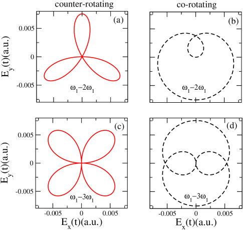
Figure 2: (Color online) Parametric plots showing the Cartesian components of the electric field vector in the $(x,y)$-polarization plane, $E_{x}(t)$ and $E_{y}(t)$, given by Eq. (3), plotted for $0\leq t\leq T_{1}$ at equal laser field intensities $I_{1}=I_{m}=10^{12}$ W/cm², ($m=2$ and $3$), for a two-color left-handed CP field in the right column with $\bm{\varepsilon}_{1}=\bm{\varepsilon}_{+}=(\mathbf{e}_{x}+i\mathbf{e}_{y})/\sqrt{2}$ and $\bm{\varepsilon_{m}}=\bm{\varepsilon}_{+}$, and a left- and right-handed CP field in the left column with $\bm{\varepsilon_{m}}=\bm{\varepsilon}_{-}$. The fundamental photon energy is $\omega_{1}=1.55$ eV while the energy of the harmonic photon is $\omega_{2}=2\omega_{1}$ in panels (a) and (b), and $\omega_{3}=3\omega_{1}$ in panels (c) and (d). The two-color bicircular electric field satisfies a $T_{1}/(m-1)$ and $T_{1}/(m+1)$ rotational symmetry for co- and counter-rotating polarizations, respectively.

for counter-rotating circular polarizations ($\bm{\varepsilon_{m}}=\bm{\varepsilon}_{-}$), in which the energies are defined by $\omega_{\pm}=\eta_{m}\,\omega_{1}/2$, where $\eta_{m}=m-1$ for corotating CP fields and $\eta_{m}=m+1$ for counter-rotating CP fields. In Fig. 2 is plotted the temporal dependence of the electric field vectors, given by Eqs. (47) and (48), in the polarization plane for two-color CP laser fields of equal intensities with identical polarizations $\bm{\varepsilon_{m}}=\bm{\varepsilon}_{+}$ in the right column, and $\bm{\varepsilon_{m}}=\bm{\varepsilon}_{-}$ in the left column. The parameters we employ for Fig. 2 are $I_{1}=I_{m}=10^{12}$ W/cm², a fundamental photon energy $\omega_{1}=1.55$ eV, with $\omega_{2}=2\omega_{1}$ in Figs. 2(a) and 2(b), and $\omega_{3}=3\omega_{1}$ in Figs. 2(c) and 2(d). The electric field vectors are invariant with respect to translation in time by an integer multiple of $T_{1}/\eta_{m}$, where $T_{1}=2\pi/\omega_{1}$ is the fundamental field optical period, and with respect to rotation in the polarization plane by an angle $\alpha_{m}=2\pi/\eta_{m}$ around the $z$ axis, such that

$${\bf E}_{\pm}\left(t+\frac{T_{1}}{\eta_{m}}\right)={\bm{R}}\left(\frac{2\pi}{\eta_{m}}\right)\,{\bf E}_{\pm}(t),$$ (49)

where ${\bm{R}}(\alpha_{m})$ is a $2\times 2$ rotation matrix with angle $\alpha_{m}$ around the $z$ axis. The upper sign (+) corresponds to corotating CP fields, while the lower sign (-) corresponds to counter-rotating CP fields. For counter-rotating bicircular field with $\omega_{2}=2\omega_{1}$, this temporal symmetry means that ${\bf E}_{-}(t+T_{1}/3)={\bm{R}}(2\pi/3)\,{\bf E}_{-}(t)$, i.e., the translation in time is one-third of the optical cycle and the rotation angle in the polarization plane is $2\pi/3$, which implies a threefold symmetry of the electric field in Fig. 2(a), while for corotating bicircular field the translation in time is $T_{1}$ and the rotation angle is $2\pi$ in Fig. 2(b), such that ${\bf E}_{+}(t+T_{1})={\bm{R}}(2\pi)\,{\bf E}_{+}(t)$.

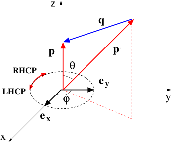
Figure 3: (Color online) Specific scattering geometry assumed for the numerical calculations of laser-assisted $e^{-}$-H($1s$) scattering in a bicircular laser field. We consider the scattering geometry with $\mathbf{p}\parallel\mathbf{e}_{z}$, where $\mathbf{p}$ and $\mathbf{p}^{\prime}$ are the momentum vectors of the incident and scattered electron, $\theta$ is the angle between them, $\varphi$ is the azimuthal angle, and $\mathbf{q}$ is the momentum transfer vector. The laser field propagates along the $z$ axis and is circularly polarized in the $(x,y)$ plane, with the polarization vectors $\bm{\varepsilon}_{+}=(\mathbf{e}_{x}+i\mathbf{e}_{y})/\sqrt{2}$ (LHCP) and $\bm{\varepsilon}_{-}=(\mathbf{e}_{x}-i\mathbf{e}_{y})/\sqrt{2}$ (RHCP).

Next, we consider the scattering geometry depicted in Fig. 3 in which the momentum vector of the incident electron $\mathbf{p}$ is parallel to the $z$ axis. The momentum transfer vector is given by $\mathbf{q}=(-p^{\prime}\sin\theta\cos\varphi,-p^{\prime}\sin\theta\sin\varphi,p-p^{\prime}\cos\theta)$, with the amplitude $q=\sqrt{p^{2}+{p^{\prime}}^{2}-2p{p^{\prime}}\cos\theta}$, where $\theta$ is the the scattering angle between the momentum vectors of the incident and scattered electron, ${\bf p}$ and ${\bf p^{\prime}}$, and $\varphi$ is the azimuthal angle of the scattered electron. In this scattering geometry the scalar product in the argument of the generalized Bessel functions, $R_{k}$, can be simply expressed as $\bm{\varepsilon}_{\pm}\cdot\mathbf{q}=-{p^{\prime}}\sin\theta/\sqrt{2}\,e^{\pm i\varphi}$. The evaluation of the dynamical phases of the CP laser fields gives $\phi_{\pm}=\pi\pm\varphi$ with $e^{i\phi_{\pm}}=-e^{\pm i\varphi}$, and we observe that a change of the field helicity implies a change in the sign of the azimuthal angle $\varphi$. After some simple algebra, by replacing the exponential term in the weak field limit of the total transition amplitudes, Eqs. (36) and (41), as $e^{-i(m\phi_{1}-\phi_{m})}=(-1)^{m+1}e^{-i\eta_{m}\varphi}$, we obtain

$$T_{m=2}(N=2)\simeq\alpha_{01}^{2}{\cal A}_{1}(\omega_{1},q)|\bm{\varepsilon}_{1}\cdot\mathbf{q}|^{2}-\alpha_{02}{\cal A}_{2}(\omega_{2},q)|\bm{\varepsilon}_{1}\cdot\mathbf{q}|e^{-i\eta_{2}\varphi},$$ (50)

for $\omega_{2}=2\omega_{1}$, with the parameter $\eta_{2}=1$ for two-color left-handed-CP fields (equal helicities) or $\eta_{2}=3$ for two-color left- and right-handed CP fields (opposite helicities), whereas for $\omega_{3}=3\omega_{1}$

$$T_{m=3}(N=2) \simeq \alpha_{01}^{2}|\bm{\varepsilon}_{1}\cdot\mathbf{q}|^{2}\left[{\cal C}_{1}(\omega_{1},q)+\frac{\alpha_{03}}{\alpha_{01}}{\cal C}_{2}(\omega_{1},\omega_{3},{q})e^{-i\eta_{3}\varphi}\right]$$ (51)

$$+\delta_{\eta_{3}2}\,\alpha_{01}\alpha_{03}\,{\cal C}_{3}(\omega_{1},\omega_{3},{q})e^{-2i\varphi},$$

with the parameter $\eta_{3}=2$ for two-color left-handed CP fields (equal helicities) or $\eta_{3}=4$ for two-color left- and right-handed CP fields (opposite helicities), respectively. Therefore, the transition amplitudes in the weak field domain, given by Eqs. (50) and (51), as well the corresponding DCSs, depend on the azimuthal angle of the scattered projectile as $e^{-i(m-1)\varphi}$ and are invariant with respect to the transformations $\varphi\to\varphi+2\pi/{(m-1)}$, for corotating polarizations. In contrast, the transition amplitudes and DCSs for counter-rotating CP fields depend on azimuthal angle as $e^{-i(m+1)\varphi}$ and are invariant with respect to the transformations $\varphi\to\varphi+2\pi/{(m+1)}$.

Furthermore, if the atomic dressing is negligible in Eqs. (50) and (51), the following simple analytic results are obtained for DCSs:

$$\frac{d{\sigma}_{m=2}(N=2)}{d\Omega}\simeq\frac{p^{\prime}}{p}\frac{(q^{2}+8)^{2}}{(q^{2}+4)^{4}}\frac{\alpha_{01}^{2}|\bm{\varepsilon}_{1}\cdot\mathbf{q}|^{2}}{16}\left|\alpha_{01}|\bm{\varepsilon}_{1}\cdot\mathbf{q}|-4\frac{\alpha_{02}}{\alpha_{01}}e^{-i\eta_{2}\varphi}\right|^{2},$$ (52)

and

$$\frac{d{\sigma}_{m=3}(N=2)}{d\Omega}\simeq\frac{p^{\prime}}{p}\frac{(q^{2}+8)^{2}}{(q^{2}+4)^{4}}\frac{\alpha_{01}^{4}|\bm{\varepsilon}_{1}\cdot\mathbf{q}|^{4}}{16}\left|1+2\frac{\alpha_{03}}{\alpha_{01}}e^{-i\eta_{3}\varphi}\right|^{2}.$$ (53)

We stress that the analytical formulas obtained for co- and counter-rotating circular polarizations in the weak-field domain, Eqs. (50) and (51), or for negligible atomic dressing, Eqs. (52) and (53), indicate that DCSs are invariant with respect to rotation of the projectile momentum in the polarization plane by azimuthal angles $2\pi/{(m-1)}$ and $2\pi/{(m+1)}$ about the $z$ axis, respectively. It is obvious that the DCS by the two-color bicircular laser field with $m=2$ in Eq. (52) presents the maximal interference between the first- and second-order transition amplitudes at the following optimal ratio of the two-color laser intensities $I_{2}/I_{1}\simeq I_{1}|\bm{\varepsilon}_{1}\cdot\mathbf{q}|^{2}/\omega_{1}^{4}$, which is very sensitive to the intensity and photon energy of the fundamental field, and the scattering geometry. In contrast, for $m=3$ the maximal interference in DCS, Eq. (53), between the second-order transition amplitudes occurs at the optimal ratio of the two-color laser intensities $I_{3}/I_{1}\simeq 20.2$, that shows the interference between the different two-photon processes is more efficient compared to $m=2$, being independent on the scattering geometry.

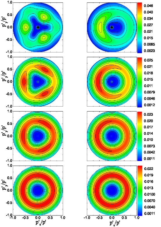
Figure 4: (Color online) Contour plots representing DCSs ($N=2$), given by Eq. (17), for a two-color left-handed CP field in the right column and a two-color left- and right-handed CP field in the left column, as a function of the normalized Cartesian components of the projectile momentum vector in the polarization plane, $p_{x}^{\prime}/{p^{\prime}}$ and $p_{y}^{\prime}/{p^{\prime}}$. The projectile electron energy is $E_{p}=100$ eV, $\textbf{p}\parallel\mathbf{e}_{z}$, and the laser field intensities are $I_{2}=I_{1},10^{-1}I_{1},10^{-2}I_{1},$ and $10^{-3}I_{1}$ from top to bottom, with $I_{1}=10^{12}$ W/cm². The photon energies are $\omega_{1}=1.55$ eV and $\omega_{2}=2\omega_{1}$. The magnitudes of the DCSs in a.u. are indicated by the color scales in each row.

First, we have checked that the two-photon DCSs for the elastic scattering of fast electrons by hydrogen atoms in their ground state are in very good agreement with the earlier analytical data obtained for the particular case of a monochromatic CP laser field acgabi2 and a bichromatic LP laser field acgabi99 . Next, we apply the analytic formulas derived in Sec. II to evaluate the DCSs for elastic electron scattering by a hydrogen atom in its ground state in the presence of two-color co- and counter-rotating CP laser fields. Since our formulas are derived up to second order in the field for the atomic dressing, we analyze two-photon absorption DCSs ($N=2$) at moderate field intensities. We choose high energies of the projectile electron and low-photon energies, such that neither the projectile electron nor the photon can separately excite an upper atomic state. To start with a simple case we present in Fig. 4 our numerical results for an initial scattering energy $E_{p}=100$ eV, photon energies that correspond to the Ti:sapphire laser $\omega_{1}=1.55$ eV and its second harmonic $\omega_{2}=2\omega_{1}$, and a fundamental laser intensity $I_{1}=10^{12}$ W/cm². These laser parameters correspond to a quiver motion amplitude $\alpha_{01}\simeq 1.65$ a.u. and an argument of the Bessel function $R_{1}\simeq 1.65|\bm{\varepsilon}_{1}\cdot{\mathbf{q}}|$. The intensity of the second-harmonic laser is given by $I_{2}=fI_{1}$, with the laser intensity ratios $f=1,10^{-1},10^{-2},$ and $10^{-3}$ from top to bottom, which results in a quiver motion amplitude $\alpha_{02}=\alpha_{01}\sqrt{f}/4$ and an argument of the Bessel function $R_{2}=R_{1}\sqrt{f}/4$. The three-dimensional electron projectile DCSs, projected in the polarization plane as a function of the normalized projectile momentum, $p_{x}^{\prime}/{p^{\prime}}$ and $p_{y}^{\prime}/{p^{\prime}}$, are plotted for two-color left-handed CP fields (corotating) in the right column and for left- and right-handed CP fields (counter-rotating) in the left column.

In the weak field domain, as long as $\omega_{1}<|E_{1s}|/2$ and $\omega_{2}=2\omega_{1}$, the one- and two-photon atomic transition matrix elements ${\cal M}_{at}^{(1)},{\cal M}_{at}^{(2)}$, and ${\cal N}_{at}^{(2)}$ are real and the DCS can be formally expressed from Eqs. (17) and (50) as a function of the scattering $\theta$ and azimuthal $\varphi$ angles,

$$\frac{d{\sigma}_{m=2}(N=2)}{d\Omega}(\theta,\varphi)\simeq a_{1}\sin^{4}\theta+a_{2}\sin^{2}\theta-a_{3}\sin^{3}\theta\cos(\eta_{2}\varphi),$$ (54)

where $a_{1}=4\pi^{4}\alpha_{01}^{4}\,{\cal A}_{1}^{2}\,p^{\prime 5}/p$, $a_{2}=8\pi^{4}\alpha_{02}^{2}\,{\cal A}_{2}^{2}\,p^{\prime 3}/p$, and $a_{3}=(2\pi)^{4}\alpha_{01}^{2}\alpha_{02}\,{\cal A}_{1}{\cal A}_{2}\,p^{\prime 4}/(p\,\sqrt{2})$. The last term in the right-side hand $a_{3}\sin^{3}\theta\cos(\eta_{2}\varphi)$, with $\eta_{2}=1$ for equal helicities and $\eta_{2}=3$ for opposite helicities, describes the coherent interference between the first- and the second-order transition amplitudes in Eq. (50), as schematically shown by the one- and two-photon pathways in Fig. 1(a). We observe that the DCS, Eq. (54), is invariant to the following transformations: (i) $\varphi\to\varphi+2\pi/\eta_{2}$, that is equivalent to a rotation in the azimuthal plane by an $2\pi/\eta_{2}$ angle around the $z$ axis and (ii) $\pi-\varphi\to\pi+\varphi$, that is equivalent to a reflection with respect to the $(x,z)$ plane.

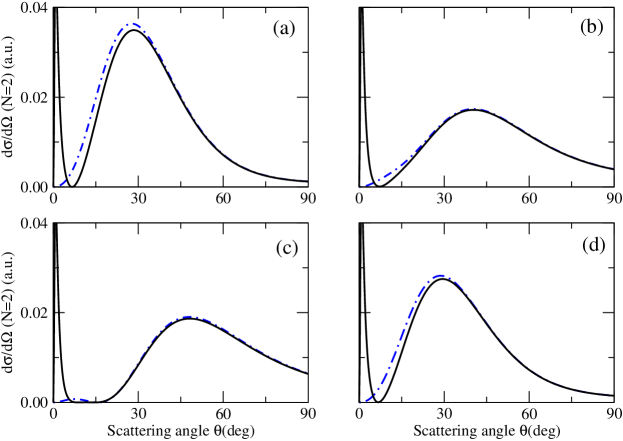
Figure 5: (Color online) Differential cross sections for $N=2$ by a two-color left- and right-handed-CP laser field in panels (a) and (c) and a two-color left-handed-CP laser field in panels (b) and (d) as a function of the scattering angle $\theta$, at the azimuthal angle $\varphi=60^{\circ}$ in panels (a) and (b), and $\varphi=240^{\circ}$ in panels (c) and (d) for $I_{1}=I_{2}=10^{12}$ W/cm². The dot-dashed lines represent the projectile electron contribution, calculated as $(2\pi)^{4}(p^{\prime}/p)|T^{(0)}(N=2)|^{2}$. The rest of the parameters are the same as in Fig. 4.

For a better understanding of the numerical results presented in Fig. 4 we show the DCSs as a function of the scattering angle $\theta$ for $I_{2}=I_{1}=10^{12}$ W/cm², at the azimuthal angles $\varphi=60^{\circ}$ in Figs. 5(a) and 5(b) and $\varphi=240^{\circ}$ in Figs. 5(c) and 5(d), while the rest of the parameters are the same as in Fig. 4. For the employed laser parameters, the laser-atom interaction is quite strong at very small scattering angles, $\theta<7^{\circ}$, only. Excepting the forward scattering angles, the projectile electron is scattered with a high probability at $\theta\simeq 40^{\circ}$ and $\theta\simeq 46^{\circ}$ in Figs. 5(a) and 5(d) and at $\theta\simeq 29^{\circ}$ in Figs. 5(b) and 5(c). At larger scattering angles, the projectile electron contribution is dominant due to nuclear scattering and determines the angular distribution of the total DCS. Very recently, there have been reported new experimental observations of the very sharp peak profile at forward scattering angles for $e^{-}$-Xe scattering in LP fields and a few attempts to explain it based on the Zon’s model Kanya2 , which involves the static polarizability.

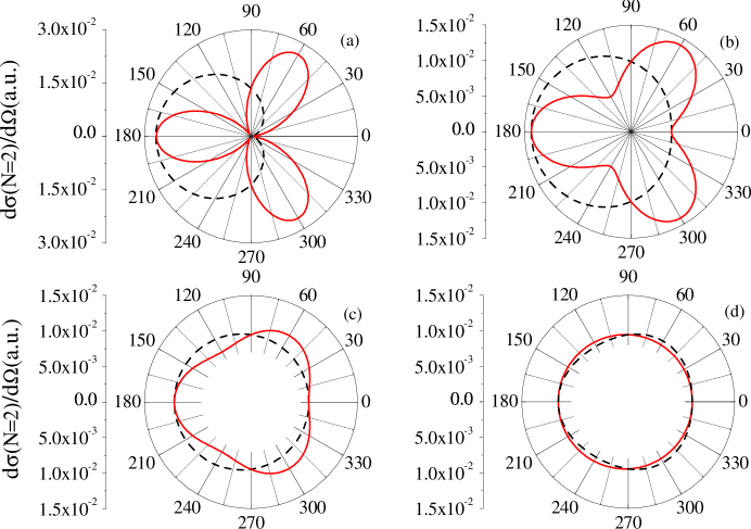
Figure 6: (Color online) Differential cross sections for $N=2$ by a two-color left- and right-handed-CP (full line) laser field and a two-color left-handed-CP (dashed line) laser field as a function of the azimuthal angle $\varphi$, at the scattering angle $\theta=20^{\circ}$, for $I_{2}=I_{1}$ in panel (a), $10^{-1}I_{1}$ in panel (b), $10^{-2}I_{1}$ in panel (c), and $10^{-3}I_{1}$ in panel (d). The rest of the parameters are the same as in Fig. 4. The DCSs by the two-color corotating CP fields are invariant to rotation by an $2\pi$ angle while by the counter-rotating CP fields are invariant to rotation by an $2\pi/3$ angle.

In order clarify the origin of the symmetry patterns in Fig. 4 for $\omega_{2}=2\omega_{1}$, we show DCSs in Fig. 6 for counter-rotating (solid lines) and corotating (dashed lines) CP fields as a function of the azimuthal angle $\varphi$, at the scattering angle $\theta=20^{\circ}$, $I_{1}=10^{12}$ W/cm², and the harmonic field intensity $I_{2}=fI_{1}$, with the laser intensity ratios $f=1$ in Fig. 6(a), $10^{-1}$ in Fig. 6(b), $10^{-2}$ in Fig. 6(c), and $10^{-3}$ in Fig. 6(d). For counter-rotating CP fields we found that the projectile electron is scattered with a high probability in the directions of the azimuthal angles $\varphi=60^{\circ},180^{\circ}$, and $300^{\circ}$. DCS has a specific “three-leaf clover”pattern, as described in the weak field domain by the $\cos 3\varphi$ term in Eq. (54), and is invariant to rotation around the $z$ axis by an azimuthal angle $\varphi=2\pi/3$. In contrast, for the corotating CP fields DCS, has a pattern described by the $\cos\varphi$ term in Eq. (54) and the invariant rotation angle is $\varphi=2\pi$. For both co- and counter-rotating CP fields, the DCSs are symmetric with respect to reflection in the $(x,z)$ plane, such that ${d{\sigma}_{m=2}}(\theta,\pi-\varphi)/{d\Omega}={d{\sigma}_{m=2}}(\theta,\pi+\varphi)/{d\Omega}$.

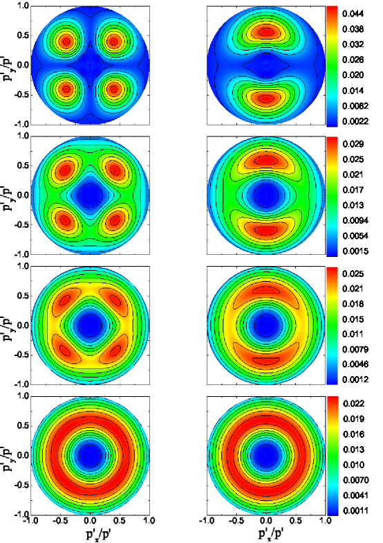
Figure 7: (Color online) Similar to Fig. 4 but for $\omega_{3}=3\omega_{1}$. The laser field intensities are $I_{3}=10I_{1},I_{1},10^{-1}I_{1},$ and $10^{-3}I_{1}$ from top to bottom, with $I_{1}=10^{12}$ W/cm². The rest of the parameters are the same as in Fig. 4. The magnitudes of the DCSs in a.u. are indicated by the color scales in each row.

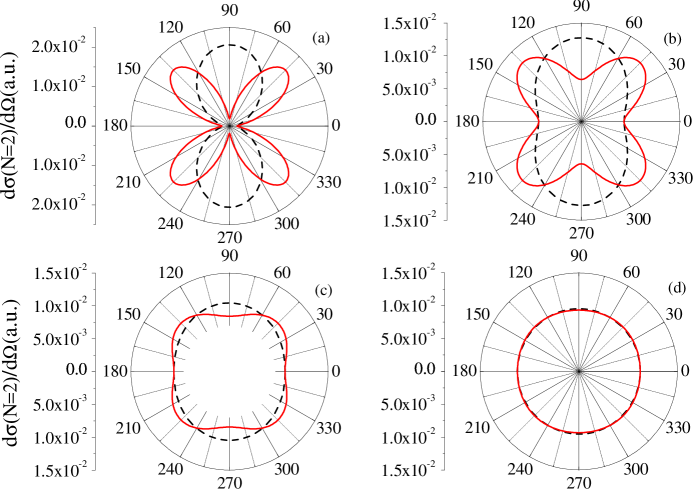
Figure 8: (Color online) Similar to Fig. 6 but for $\omega_{3}=3\omega_{1}$, at $I_{3}=10I_{1}$ in panel (a), $I_{1}$ in panel (b), $10^{-1}I_{1}$ in panel (c), and $10^{-3}I_{1}$ in panel (d). The rest of the parameters are the same as in Fig. 4. The DCSs by the two-color corotating CP fields are invariant to rotation by an $\pi$ angle while by the counter-rotating CP fields are invariant to rotation by an $\pi/2$ angle.

Figure 7 presents similar results as in Fig. 4 but for a combination of the fundamental laser field and its third harmonic, $\omega_{3}=3\omega_{1}$, which results in the quiver motion amplitude $\alpha_{03}=\alpha_{01}\sqrt{f}/9$ and the argument of the Bessel function $R_{3}=R_{1}\sqrt{f}/9$. In order to understand the different symmetry patterns in Fig. 7, we show DCSs in Fig. 8 for counter-rotating (solid lines) and corotating (dashed lines) CP fields as a function of the azimuthal angle $\varphi$, at the scattering angle $\theta=20^{\circ}$, and the harmonic field intensity $I_{3}=fI_{1}$, with laser intensity ratios $f=10$ in Fig. 8(a), $1$ in Fig. 8(b), $10^{-1}$ in Fig. 8(c), and $10^{-3}$ in Fig. 8(d). In contrast with the $\omega_{2}=2\omega_{1}$ case we found that the projectile electron is scattered with a high probability in the directions of the azimuthal angles $\varphi=45^{\circ},135^{\circ},225^{\circ}$, and $315^{\circ}$ for counter-rotating CP fields. DCS has a “four-leaf clover”pattern which is described in the weak field domain, Eqs. (51) and (53), by a $\cos 4\varphi$ term and is invariant to rotation around the $z$ axis by an azimuthal angle $\varphi=\pi/2$ for counter-rotating CP fields. For corotating CP fields, DCS has a specific pattern described by $\cos 2\varphi$ and the invariant rotation angle is $\varphi=\pi$. The DCSs for co- and counter-rotating polarizations are symmetric with respect to reflection in the $(x,z)$- and $(y,z)$-planes, such that ${d{\sigma}_{m=3}}(\theta,\pi-\varphi)/{d\Omega}={d{\sigma}_{m=3}}(\theta,\pi+\varphi)/{d\Omega}$ and ${d{\sigma}_{m=3}}(\theta,\pi/2-\varphi)/{d\Omega}={d{\sigma}_{m=3}}(\theta,\pi/2+\varphi)/{d\Omega}$, respectively. Recently, three-dimensional electron distributions with one and three lobes were experimentally observed in strong-field ionization by two-color CP fields Mancuso15 , using a superposition of fundamental and second harmonic of a Ti:sapphire laser. Similar rotational and reflection symmetries were obtained in above-threshold detachment of negative fluorine ions by a two-color bicircular laser field Odzak .

As expected, at relatively low harmonic intensities $I_{m}\ll I_{1}$ ($m=2,3$), where the one-color ($\omega_{1}$) two-photon processes are dominating, the DSCs are almost independent on the azimuthal angle $\varphi$ and have nearly circularly symmetric patterns in the polarization plane acgabi2 , as shown in Figs. 4 and 7 and at $\theta=20^{\circ}$ in Figs. 6(d) and 8(d) for two left-handed-CP pulses and two left- and right-handed-CP pulses, respectively. In conclusion, the DCSs presented in Fig. 4 and Figs. 6-8 for both co- and counter-rotating CP fields have different interference patterns between the different paths leading to the same final state and have almost the same peak magnitude. The counter-rotating circular polarization case has a different symmetry profile and obeys different symmetry operations: The DCS is invariant to rotation of the projectile electron momentum around the $z$ axis by an angle $2\pi/(m+1)$ for counter-rotating CP fields, whereas for the corotating CP fields the invariant rotation angle is $2\pi/(m-1)$.

V Summary and conclusions

Using a semiperturbative method, we have studied the electron-hydrogen scattering by a two-color CP laser field of commensurate photon energies $\omega_{1}$ and $m\omega_{1}$, and derived useful analytical formulas for DCSs that are valid for circular and/or linear polarization and give more physical insight of the scattering process and valuable information for experimental investigations. A comparison between the two-photon absorption DCSs for two-color co- and counter-rotating CP laser fields is made at different photon energies of the harmonic field $2\omega_{1}$ and $3\omega_{1}$ ($m=2$ and $3$), and the effect of the intensity ratio of the two-color laser field components on the DCSs is analyzed. The DCSs of the scattered electrons by hydrogen atoms in a two-color bicircular laser field of photon energies $\omega_{1}$ and $m\omega_{1}$ present a rotational symmetry with respect to rotation of the projectile electron momentum by an azimuthal angle $2\pi/(m-1)$ for corotating polarizations, while for counter-rotating polarizations the invariant rotation angle is $2\pi/(m+1)$. In addition to the rotational symmetry, for the studied scattering geometry $\bm{\varepsilon}_{\pm}=(\mathbf{e}_{x}\pm i\mathbf{e}_{y})/\sqrt{2}$ and $\bf p\parallel\mathbf{e}_{z}$, the DCSs are symmetric with respect to reflection in the $(x,z)$ plane for both $m=2$ and $3$, while the $(y,z)$ plane is a reflection symmetry plane for $m=3$ only. It was found that the modification of the photon helicity implies a change in the symmetries of the DCSs and by changing the laser field intensity ratio the angular distribution of the scattering signal can be modified. By choosing the photon energies ratio to be even ($m=2$) or odd ($m=3$) and varying the intensity ratio of the co- and counter-rotating two-color CP laser field components we can manipulate the angular distribution of the scattered electrons. The optimization of the scattering signal in laser-assisted electron-hydrogen scattering process depends for $\omega_{3}=3\omega_{1}$ on the intensity ratio of the two-color laser field components, whereas for $\omega_{2}=2\omega_{1}$ depends on the scattering geometry, fundamental field intensity, and photon energy.

Appendix A SECOND-ORDER CORRECTION TO THE ATOMIC WAVE FUNCTION FOR A TWO-COLOR LASER FIELD

In order to calculate the second-order atomic transition amplitude, Eq. (27), we use the expression of the quadratic response tensors defined in Ref. vf2 for the two-color laser field given by Eq. (2) to obtain the second-order correction to the atomic ground state as

$$\psi_{1s}^{(2)}(\mathbf{r},t) = \sum_{k=1,m}\frac{\alpha_{0k}^{2}\omega_{k}^{2}}{4}\sum_{j,l=1}^{3}\left[\varepsilon_{kj}\varepsilon_{kl}\;w_{jl,100}(\Omega_{k}^{\prime\,+},\Omega_{k}^{+};\mathbf{r})e^{-2i\omega_{k}t}+\varepsilon_{kj}^{*}\varepsilon_{kl}^{*}\;w_{jl,100}(\Omega_{k}^{\prime\,-},\Omega_{k}^{-};\mathbf{r})e^{2i\omega_{k}t}\right.$$ (55)

$$\left.+\varepsilon_{kj}\varepsilon_{kl}^{*}\;\widetilde{w}_{jl,100}(E_{1s},\Omega_{k}^{-};\mathbf{r})+\varepsilon_{kj}^{*}\varepsilon_{kl}\;\widetilde{w}_{jl,100}(E_{1s},\Omega_{k}^{+};\mathbf{r})\right]$$

$$+\frac{\alpha_{01}\alpha_{0m}\omega_{1}\omega_{m}}{4}\sum_{j,l=1}^{3}\left\{\varepsilon_{1j}\varepsilon_{ml}[w_{lj,100}(\Omega^{\prime\,+},\Omega_{1}^{+};\mathbf{r})+w_{jl,100}(\Omega^{\prime\,+},\Omega_{m}^{+};\mathbf{r})]e^{-i(\omega_{1}+\omega_{m})t}\right.$$

$$+\varepsilon_{1j}^{*}\varepsilon_{ml}^{*}[w_{lj,100}(\Omega^{\prime\,-},\Omega_{1}^{-};\mathbf{r})+w_{jl,100}(\Omega^{\prime\,-},\Omega_{m}^{-};\mathbf{r})]e^{i(\omega_{1}+\omega_{m})t}$$

$$+\varepsilon_{1j}\varepsilon_{ml}^{*}[w_{lj,100}(\Omega^{+},\Omega_{1}^{+};\mathbf{r})+w_{jl,100}(\Omega^{+},\Omega_{m}^{-};\mathbf{r})]e^{-i(\omega_{1}-\omega_{m})t}$$

$$\left.+\varepsilon_{1j}^{*}\varepsilon_{ml}[w_{lj,100}(\Omega^{-},\Omega_{1}^{-};\mathbf{r})+w_{jl,100}(\Omega^{-},\Omega_{m}^{+};\mathbf{r})]e^{i(\omega_{1}-\omega_{m})t}\right\},$$

where the tensors $w_{jl,100}$ and $\widetilde{w}_{jl,100}$ are defined by Eqs. (10) and (11), and the energy parameters are $\Omega_{k}^{\pm}=E_{1s}\pm\omega_{k}$, $\Omega_{k}^{\prime\,\pm}=E_{1s}\pm 2\omega_{k}$, $\Omega^{\pm}=E_{1s}\pm(\omega_{1}-\omega_{m})$, and $\Omega^{\prime\,\pm}=E_{1s}\pm(\omega_{1}+\omega_{m})$, with $k=1$ and $m$.

Appendix B APPROXIMATE FORMULA FOR THE GENERALIZED BESSEL FUNCTIONS $B_{N}(R_{1},R_{m},\phi_{1},\phi_{m})$

We recall the definition introduced in Subsec. II.2 of the phase-dependent generalized Bessel function for commensurate photon energies $\omega_{1}$ and $\omega_{m}=m\omega_{1}$,

$$B_{N}(R_{1},R_{m};\phi_{1},\phi_{m})=\sum_{l=-\infty}^{+\infty}J_{N-ml}(R_{1})J_{l}(R_{m})\exp{[-il(m\phi_{1}-\phi_{m})]},$$ (56)

which is a $2\pi$ periodic function in $\phi_{1}/m$ and $\phi_{m}$ varro . Whenever the argument of the Bessel functions of the first kind is small, i.e., $R_{1}\ll 1$ and $R_{m}\ll 1$, which is satisfied at low laser intensities or at small scattering angles with moderate laser intensities, the approximate expressions of the generalized Bessel functions can be used. In the present paper we keep the second-order terms in the fields in the transition amplitudes and, therefore, we restrict to the following approximate formula:

$$B_{N}\simeq J_{N}(R_{1})J_{0}(R_{m})+J_{N-m}(R_{1})J_{1}(R_{m})e^{-i(m\phi_{1}-\phi_{m})},\quad\text{for \; $N\geq 0$}.$$ (57)

Using the approximate relation $J_{N}(R_{k})\simeq R_{k}^{N}/(2^{N}{N!})$ and the symmetry formula $J_{-N}(R_{k})=(-1)^{N}J_{N}(R_{k})$ of the Bessel functions of the first kind Watson , we further obtain

$$B_{N}\simeq\frac{R_{1}^{N}}{2^{N}N!}+\frac{(\beta R_{1})^{|N-m|}R_{m}}{2^{|N-m|+1}\;|N-m|!}e^{-i(m\phi_{1}-\phi_{m})},\quad\text{for \; $N\geq 0$},$$ (58)

where $\beta=-1$ for $0<N<m$ and $\beta=1$ for $N\geq m$. Because the appropriate leading terms are kept in the total transition amplitude in the weak field domain, Eq. (35), the following approximate expressions are used for two-photon absorption scattering process: $B_{0}\simeq 1$, $B_{1}\simeq R_{1}/2$, $B_{2}\simeq R_{1}^{2}/8+(\beta R_{1}/2)^{|2-m|}(R_{m}/2)e^{-i(m\phi_{1}-\phi_{m})}/|2-m|!$, and $B_{N}\simeq 0$ for $N\geq 3$. Explicitly, for $N=2$ the generalized Bessel function is approximated as

$$B_{2}\simeq\begin{cases}[\alpha_{01}^{2}(\bm{\varepsilon}_{1}\cdot\mathbf{q})^{2}+4\alpha_{02}\,\bm{\varepsilon}_{2}\cdot\mathbf{q}]\,e^{-i2\phi_{1}}/8,&\quad\text{for \; $m=2$},\\ [\alpha_{01}^{2}(\bm{\varepsilon}_{1}\cdot\mathbf{q})^{2}-2\alpha_{01}\alpha_{03}(\bm{\varepsilon}_{1}^{*}\cdot\mathbf{q})(\bm{\varepsilon}_{3}\cdot\mathbf{q})]\,e^{-i2\phi_{1}}/8,&\quad\text{for \; $m=3$}.\end{cases}$$ (59)

Similar results can be obtained for $N<0$ by using the symmetry relation for $B_{-N}$,

$$B_{-N}(R_{1},R_{m};\phi_{1},\phi_{m})=(-1)^{N}B_{N}^{\mbox{*}}[R_{1},R_{m};\phi_{1},\phi_{m}+(m-1)\pi].$$

For odd harmonic orders, such that $m=2s+1$, with $s$ being a positive integer, the following symmetry relation occurs: $B_{-N}(R_{1},R_{m};\phi_{1},\phi_{m})=(-1)^{N}B_{N}^{\mbox{*}}(R_{1},R_{m};\phi_{1},\phi_{m})$. For even harmonic orders, such that $m=2s$, the following symmetry relation holds: $B_{-N}(R_{1},R_{m};\phi_{1},\phi_{m})=(-1)^{N}B_{N}^{\mbox{*}}(R_{1},R_{m};\phi_{1},\phi_{m}+\pi)$.

Figure 1: Energy diagrams schematically showing the channels leading to the final energy of the projectile electron $E_{p\prime}=E_{p}+2\omega_{1}$. Channel (a) corresponds to absorption of two photons of energy $\omega_{1}$ and one photon of energy $\omega_{2}=2\omega_{1}$ of the second harmonic, while channel (b) corresponds to absorption of two photons of energy $\omega_{1}$ and absorption of the third harmonic $\omega_{3}=3\omega_{1}$ and emission of the photon $\omega_{1}$.

References

• (1) F. Ehlotzky, Phys. Rep. 345, 175 (2001).
• (2) Y. Shima and H. Yatom, Phys. Rev. A 12, 2106 (1975); M. B. S. Lima, C. A. S. Lima, and L. C. M. Miranda, ibid. 19, 1796 (1979).
• (3) S. Chandrasekhar, An Introduction to the Study of Stellar Structure, (Dover, Mineola, NY, 1967), p. 261; M. J. Seaton, in Advances in Atomic, Molecular and Optical Physics edited by B. Bederson and A. Dalgarno (Academic Press, New York, 1994), p. 395.
• (4) N. F. Mott and H. S. W. Massey, The Theory of Atomic Collisions (Oxford University Press, London, 1965); C. Joachain, Quantum Collision Theory (North Holland, Amsterdam, 1987).
• (5) N. J. Mason, Rep. Prog. Phys. 56, 1275 (1993).
• (6) F. Ehlotzky, A. JaroΕ„, and J. Z. KamiΕ„ski, Phys. Rep. 297, 63 (1998).
• (7) B. H. Bransden and C. J. Joachain, Physics of Atoms and Molecules (Longman, London, 1983).
• (8) C. J. Joachain, N. J. Kylstra, and R. M. Potvliege, Atoms in Intense Laser Fields (Cambridge University Press, Cambridge, UK, 2012), p. 466.
• (9) M. O. Musa, A. MacDonald, L. Tidswell, J. Holmes, and B. Wallbank, J. Phys. B: At. Mol. Phys. 43, 175201 (2010).
• (10) R. Kanya, Y. Morimoto, and K. Yamanouchi, Phys. Rev. Lett. 105, 123202 (2010).
• (11) B. A. de Harak, L. Ladino, K. B. MacAdam, and N. L. S. Martin, Phys. Rev. A 83, 022706 (2011).
• (12) Y. Morimoto, R. Kanya, and K. Yamanouchi, Phys. Rev. Lett. 115, 123201 (2015); R. Kanya, Y. Morimoto, and K. Yamanouchi, in Progress in Ultrafast Intense Laser Science X, edited by K. Yamanouchi, G. Paulus, and D. Mathur (Springer, Cham, Switzerland, 2014), p. 1.
• (13) G. Buica, Phys. Rev. A 92, 033421 (2015); J. Quant. Spectrosc. Radiat. Transf. 187, 190 (2017).
• (14) S. Long, W. Becker, and J. K. McIver, Phys. Rev. A 52, 2262 (1995).
• (15) H. Eichmann, A. Egbert, S. Nolte, C. Momma, B. Wellegehausen, W. Becker, S. Long, and J. K. McIver, Phys. Rev. A 51, R3414 (1995).
• (16) A. Fleischer, O. Kfir, T. Diskin, P. Sidorenko, and O. Cohen, Nat. Photon. 8, 543 (2014).
• (17) C. A. Mancuso, D. D. Hickstein, P. Grychtol, R. Knut, O. Kfir, X. M. Tong, F. Dollar, D. Zusin, M. Gopalakrishnan, C. Gentry, E. Turgut, J. L. Ellis, M. C. Chen, A. Fleischer, O. Cohen, H. C. Kapteyn, and M. M. Murnane, Phys. Rev. A 91, 031402(R) (2015).
• (18) C. A. Mancuso, K. M. Dorney, D. D. Hickstein, J. L. Chaloupka, J. L. Ellis, F. J. Dollar, R. Knut, P. Grychtol, D. Zusin, C. Gentry, M. Gopalakrishnan, H. C. Kapteyn, and M. M. Murnane, Phys. Rev. Lett. 117, 133201 (2016).
• (19) S. OdΕΎak and D. B. MiloΕ‘eviΔ‡, Phys. Rev. A 92, 053416 (2015).
• (20) S. OdΕΎak, E. HasoviΔ‡, W. Becker, and D. B. MiloΕ‘eviΔ‡, J. Mod. Opt. 64, 971 (2017).
• (21) A. Cionga, F. Ehlotzky, and G. Zloh, Phys. Rev. A 61, 063417 (2000).
• (22) A. Cionga, F. Ehlotzky, and G. Zloh, Phys. Rev. A 62, 063406 (2000); J. Phys. B: At. Mol. Opt. Phys. 33, 4939 (2000).
• (23) F. W. Byron Jr. and C. J. Joachain, J. Phys. B 17, L295 (1984).
• (24) D. M. Volkov, Z. Phys. 94, 250 (1935).
• (25) V. Florescu and T. Marian, Phys. Rev. A 34, 4641 (1986).
• (26) V. Florescu, A. Halasz, and M. Marinescu, Phys. Rev. A 47, 394 (1993).
• (27) G. N. Watson, Theory of Bessel Functions (Cambridge University Press, Cambridge, UK, 1962).
• (28) S. VarrΓ³ and F. Ehlotzky, J. Phys. B: At. Mol. Opt. Phys. 28, 1613 (1995).
• (29) F. V. Bunkin and M. V. Fedorov, Zh. Eksp. Teor. Fiz., 49, 1215 (1965) [Sov. Phys. JETP 22, 844 (1966)].
• (30) D. B. MiloŝeviΔ‡, F. Ehlotzky, and B. Piraux, J. Phys. B 30, 4347 (1997).
• (31) A. Cionga, F. Ehlotzky, and G. Zloh, Phys. Rev. A 64, 043401 (2001).
• (32) M. Gavrila and A. Costescu, Phys. Rev. A 2, 1752 (1970).
• (33) V. Veniard, M. Gavrila, and A. Maquet, Phys. Rev. A 35, 448(R) (1987); A. A. KrylovetskiΔ­, N. L. Manakov, S. I. Marmo, and A. F. Starace, J. Exp. Theor. Phys. 95, 1006 (2002).
• (34) N. L. Manakov, A. V. Meremianin, J. P. J. Carney, and R. H. Pratt, Phys. Rev. A 61, 032711 (2000).
• (35) R. Taieb, V. Veniard, A. Maquet, N. L. Manakov, and S. I. Marmo, Phys. Rev. A 62, 013402 (2000).
• (36) M. Fifirig, V. Florescu, A. Maquet, and R. TaΓ―eb, J. Phys. B: At. Mol. Opt. Phys. 33, 5313 (2000); M. Fifirig, A. Cionga, and F. Ehlotzky, Eur. Phys. J. D 23, 333 (2003).
• (37) A. Y. Istomin, E. A. Pronin, N. L. Manakov, S. I. Marmo, and A. F. Starace, Phys. Rev. Lett. 97, 123002 (2006).
• (38) A. Cionga and G. Zloh, Laser Phys. 9, 69 (1999).
Refer to caption