Polarization dependence in inelastic scattering of electrons by hydrogen atoms in a circularly polarized laser field

Abstract

We theoretically study the influence of laser polarization in inelastic scattering of electrons by hydrogen atoms in the presence of a circularly polarized laser field in the domain of field strengths below $10^{7}$ V/cm and high projectile energies. A semi-perturbative approach is used in which the interaction of the projectile electrons with the laser field is described by Gordon-Volkov wave functions, while the interaction of the hydrogen atom with the laser field is described by first-order time-dependent perturbation theory. A closed analytical solution is derived in laser-assisted inelastic electron-hydrogen scattering for the $1s\to nl$ excitation cross section which is valid for both circular and linear polarizations. For the excitation of the $n=2$ levels simple analytical expressions of differential cross section are derived for laser-assisted inelastic scattering in the perturbative domain, and the differential cross sections by the circularly and linearly polarized laser fields and their ratios for one- and two-photon absorption are calculated as a function of the scattering angle. Detailed numerical results for the angular dependence and the resonance structure of the differential cross sections is discussed for the $1s\to 4l$ excitations of hydrogen in a circularly polarized laser field.

1 Introduction

It is well known that the atomic processes which take place in the presence of an electromagnetic field and involve atomic spectra exhibit field polarization-dependent characteristics [1]. Obviously polarization dependence effects occur as well for electron-atom scattering in the presence of a laser field, which is of potential interest in applied domains such as laser and plasma physics [2], astrophysics [3], or fundamental atomic collision theory [4]. Detailed reports on the laser-assisted electron-atom collisions can be found in several review papers [5, 6, 7] and books [8, 9]. The polarization dependence of elastic laser-assisted electron-hydrogen scattering was first theoretically studied for circularly polarized (CP) fields and differences between the angular distributions for linear and circular polarizations were reported by Fainstein and Maquet [10], by considering a model potential for the calculation of the atomic wave functions. Theoretical studies involving CP fields with the atomic dressing taken into account in second-order of time-dependent perturbation theory (TDPT) were performed for elastic case by Cionga and coworkers [11, 12], and the dichroism of the scattered electrons was investigated in elastic electron-hydrogen scattering by circularly and elliptically polarized laser fields [13]. The polarization effects in laser-assisted electron-atom inelastic collisions for the excitation of the $n=2$ and $3$ states in H and He, were reported [14] for two specific scattering geometries where the wave vector of the CP field is coplanar and parallel to the scattering plane. A different method based on a discrete basis of Sturmian functions was employed to calculate the relevant atomic terms of the scattering matrix and, in contrast to this previous treatment, a major purpose of our paper is to provide new analytical formulas needed to compute the differential cross section (DCS) for the laser-assisted excitation collisions $e^{-}+H({1s})$ by CP laser fields, that allow further investigations of the polarization effect and give more insight into the scattering process. It is well known that by increasing the atomic excitation the laser-dressing effects induced by the dipole polarizability [15] should increase in importance [16, 17, 18], and therefore with an increasing probability of experimental detection. As far as we known the first theoretical works on the laser-assisted inelastic scattering of electrons by atoms taking into account the atomic “dressing” (i.e., the dipole distortion of the atom by the laser field) were performed in different approaches such as first-order perturbation theory [19, 20, 21, 22], non-perturbative Floquet theory [23], or relativistic method [24].

Similarly to the case of elastic collisions, most experimental investigations of inelastic electron-atom scattering are focused on collision processes in linearly polarized (LP) laser fields [5]. The first experimental observation of an inelastic process involving one-photon absorption was made by Mason and Newell for electron-helium scattering in elliptically [25] and circularly [26] polarized laser fields. In the recent years due to progresses in new experimental techniques there is a renewed interest in investigating electron-atom scattering in the presence of a laser field [27, 28, 29, 30], and therefore there is a need for simple analytical formulas in order to describe the process. Very recently, there is also an increased interest in the simultaneous electron-photon excitation of helium in the presence of a laser field using a nonperturbative R-matrix Floquet theory [31], or involving a semi-perturbative method in the second-order Born approximation [32].

In this paper we investigate the $1s\rightarrow nl$ inelastic scattering of fast electrons by hydrogen atoms in their ground states in the presence of a CP laser field. In Sec. 2 is described the semi-perturbative framework used to derive the analytical formulas for the DCS for excitation of an arbitrary state. Because the scattering process under investigation is a very complex problem, the theoretical approach poses considerable difficulties and several assumptions are made. (i) Moderate laser field strengths below $10^{7}$ V/cm and fast projectile electrons are considered in order to safely neglect the second-order Born approximation in the scattering potential as well as the exchange scattering [33, 20, 34]. (ii) The interaction of the projectile electrons with the laser field is described by a Gordon-Volkov wave function [35]. (iii) The dressing of the hydrogen atom by the laser field is described within the first-order time-dependent perturbation theory (TDPT) in the field [36]. This theoretical approach is similar to the one that has been used to a related problem of laser-assisted excitation collisions $e^{-}+H({2s})$ by LP laser fields [18] and, contrasting with this work, the main differences reside in the initial atomic state, that is now ${1s}$, and the circular polarization of the laser field, which result in different specific expressions for the projectile and atomic contributions to DCS by CP fields. In comparison to the earlier theoretical works [20, 22, 14] the present semi-perturbative approach provides, for the first-time as far as we know, a closed analytical form for the DCS, which includes the atomic dressing effects, and is valid for both LP and CP fields. We obtain useful analytic formulas for DCSs in the laser-assisted inelastic scattering in the perturbative limit as well in the soft-photon limit for the $1s\to nl$ excitation. Simple asymptotic formulas for DCS are derived at low-photon energies for the $1s\to 2s$ and $1s\to 2p$ excitations. Section 3 is devoted to discussion of the numerical results, where the angular distributions of the DCSs by CP fields are presented for the excitation of $n=2$ and $4$ subshells, and the resonance structure of the DCSs as a function of the photon energy is analyzed for the excitation of $n=4$ subshells. The ratios of the differential cross sections by the CP and LP laser fields are calculated as a function of the scattering angle for the excitation of $n=2$ subshells accompanied by one- and two-photon absorption, which could be very useful from the experimental point of view. Atomic units (a.u.) are used throughout this paper unless otherwise specified.

2 Semi-perturbative scattering theory at moderate laser intensities and circular polarizations

We consider the following laser-assisted inelastic scattering of electrons by hydrogen atoms in their ground state (free-free transitions):

$$e^{-}(E_{k_{i}},{\mathbf{k}_{i}})+{\rm H}(1s)+N_{i}\;\gamma\;(\omega,\bm{\varepsilon})\to e^{-}(E_{k_{f}},{\mathbf{k}_{f}})+{\rm H}(nlm)+N_{f}\;\gamma\;(\omega,\bm{\varepsilon}),$$ (1)

where $E_{k_{i}}\;(E_{k_{f}})$ and $\mathbf{k}_{i}\;(\mathbf{k}_{f}$) denote the kinetic energy and the momentum vector of the projectile electron in its initial (final) state. $\gamma$ denotes a photon with the energy $\omega$ and the polarization vector $\bm{\varepsilon}$. The hydrogen atom is initially in its ground state and finally is excited to a final state defined by the quantum numbers $n,l$, and $m$. The above scattering process is considered inelastic since the initial and final states of the target are not identical and therefore the projectile electron energies satisfy the conservation relation: $E_{k_{f}}=E_{k_{i}}+{E}_{1s}-{E}_{n}+N\omega$, where ${E}_{1s}$ and ${E}_{n}$ are the energies of the ground and excited states, and $N=N_{i}-N_{f}$ denotes the net number of exchanged photons between the colliding system and the laser field. The kinetic energy spectrum of the scattered electrons consists of a central line that corresponds to $N=0$ and a number of symmetrically located sideband lines with $|N|=1,2,3,$…, equally spaced by the photon energy [5]. The laser field is assumed to be a monochromatic electric field and is treated classically as

$$\mbox{\boldmath$\cal E$}(t)=\frac{i}{2}{\cal E}_{0}\bm{\varepsilon}\exp(-i\omega t)+cc,$$ (2)

where ${\cal E}_{0}$ is the peak amplitude of the electric field, and the polarization vector is given by

$$\bm{\varepsilon}=\cos(\xi/2)[\mathbf{e}_{i}+i\mathbf{e}_{j}\tan(\xi/2)],$$ (3)

where $\mathbf{e}_{i}$ and $\mathbf{e}_{j}$ are the unit vectors along two orthogonal directions in the polarization plane and $\xi$ denotes the ellipticity degree. In particular, the ellipticity is $\xi=\pm\pi/2$ for a CP field and $\xi=0$ for a LP field.

2.1 Scattering matrix in the semi-perturbative domain

As stated previously, in the present work we consider fast projectile electrons such that the scattering process can be well treated within the first-order Born approximation in the scattering potential

$$V(r,R)=-\frac{1}{R}+\frac{1}{|\bf{R}-\bf{r}|},$$ (4)

where $\mathbf{R}$ and $\mathbf{r}$ denote the position vectors of the projectile and bound electrons, and we use a semi-perturbative approach for the scattering process similar to the one developed by Byron and Joachain [33]. We start with the calculation of the scattering matrix element [20] in the domain of high scattering energies as

$$S_{fi}=-i\int_{-\infty}^{\infty}dt\langle\chi_{\mathbf{k}_{f}}(\mathbf{R},t)\Psi_{n_{f}l_{f}m_{f}}(\mathbf{r},t)|V(\mathbf{r},\mathbf{R})|{\chi}_{\mathbf{k}_{i}}(\mathbf{R},t)\Psi_{n_{i}l_{i}m_{i}}(\mathbf{r},t)\rangle\;,$$ (5)

where $\chi_{\mathbf{k}_{i}}$ and $\chi_{\mathbf{k}_{f}}$ represent the initial and final Gordon-Volkov wave functions of the projectile electron in the laser field, and $\Psi_{n_{i}l_{i}m_{i}}$ and $\Psi_{n_{f}l_{f}m_{f}}$ are the initial and final wave functions of the bound electron in the laser field, which are given by Eqs. (3) and (5) of Ref. [18]. For fast projectile electrons ($E_{k_{i}}>150$ eV) the exchange effects are safely neglected [20] and are not included in the calculation of the scattering matrix. As long as the laser field strength remains moderate the interaction of the hydrogen atom with the laser field is considered within the first-order TDPT. More details about the dressing effects are discussed elsewhere [11, 12, 17]. By using the Jacob-Anger expansion of the exponential

$$\exp{[iX\sin(\omega t)]}=\sum_{N=-\infty}^{+\infty}J_{N}(X)\exp{(iN\omega t)},$$ (6)

we develop the Gordon-Volkov wave functions in terms of the ordinary Bessel functions [38] of order $N$, $J_{N}$,

$$\exp{[-i\bm{\alpha}(t)\cdot\mathbf{k}]}=\sum_{N=-\infty}^{+\infty}J_{N}(X_{k})\exp{(-iN\omega t+iN\phi_{k})},$$ (7)

where $X_{k}=\alpha_{0}|\bm{\varepsilon}\cdot\mathbf{k}|$ is the argument of the Bessel function and the dynamical phase $\phi_{k}$ is defined through the expression $\exp{(i\phi_{k})}=|\bm{\varepsilon}\cdot\mathbf{k}|/(\bm{\varepsilon}\cdot\mathbf{k})$. The quiver motion of the projectile electron in the electric field $\mbox{\boldmath$\cal E$}(t)$, Eq. (2), is described by

$$\bm{\alpha}(t)={\alpha_{0}}[\mathbf{e}_{i}\sin(\omega t)\cos(\xi/2)-\mathbf{e}_{i}\cos(\omega t)\sin(\xi/2)],$$ (8)

with the amplitude ${\alpha_{0}}={\cal E}_{0}/\omega^{2}$. For a CP field $X_{k}^{CP}=(\alpha_{0}/\sqrt{2})\sqrt{(\mathbf{e}_{i}\cdot\mathbf{k})^{2}+(\mathbf{e}_{j}\cdot\mathbf{k})^{2}}$ and $\phi_{k}^{CP}=\arctan{(\mathbf{e}_{j}\cdot\mathbf{k})/(\mathbf{e}_{i}\cdot\mathbf{k})}+s\pi$, while for a LP field $X_{k}^{LP}=\alpha_{0}|\mathbf{e}_{i}\cdot\mathbf{k}|$ and $\phi_{k}^{LP}=s\pi$, where $s$ is an integer. By substituting the projectile and atomic wave functions into Eq. (5) we obtain, after integrating over time and projectile coordinate, the scattering matrix $S_{fi}$ for the laser-assisted inelastic electron-hydrogen collisions accompanied by the exchange of $N$ photons (absorbed or emitted),

$$S_{fi}(N)=-2\pi i\sum_{N=-\infty}^{+\infty}T_{nlm}(N)\;\delta(E_{k_{f}}+{E}_{n}-E_{k_{i}}-{E}_{1s}-N\omega)\;,$$ (9)

where $\delta$ is the Dirac delta function which is related to the energy conservation $E_{k_{f}}=E_{k_{i}}+{E}_{1s}-{E}_{n}+N\omega$. $T_{nlm}(N)$ denotes the total transition amplitude for the scattering process (1), which can be split as a sum of two terms:

$$T_{nlm}(N)=T_{nlm}^{(0)}(N)+T_{nlm}^{(1)}(N).$$ (10)

The first term on the right-hand side of Eq. (10), $T_{nlm}^{(0)}$, represents the inelastic transition amplitude due to projectile electron, and describes the direct excitation of hydrogen by projectile electron interaction,

$$T_{nlm}^{(0)}(N)=J_{N}(X_{q})\langle\psi_{nlm}|F(\mathbf{q})|\psi_{100}\rangle,$$ (11)

where $\psi_{nlm}$ is the unperturbed excited-state wave function of the bound electron, $X_{q}=\alpha_{0}|\bm{\varepsilon}\cdot{\mathbf{q}}|$, and $\mathbf{q}=\mathbf{k}_{i}-\mathbf{k}_{f}$ denotes the momentum transfer vector of the projectile electron. $F(\mathbf{q})$ represents the generalized form factor given by

$$F(\mathbf{q})=\frac{1}{2\pi^{2}q^{2}}\left[\exp{(i\mathbf{q}\cdot\mathbf{r})}-\delta_{n1}\delta_{l0}\delta_{m0}\right].$$ (12)

The laser and the projectile contributions to the transition amplitude $T_{nlm}^{(0)}$, are completely decoupled in Eq. (11) because the laser-field dependence of the electronic transition amplitude is included in the argument of the Bessel function only. We recall that the Bunkin-Fedorov [39] and Kroll-Watson [40] formulas are inappropriate for laser-assisted inelastic electron-atom scattering (in which the atom changes its initial state) since both approximations are obtained for a static potential.

The second term on the right-hand side of the inelastic transition amplitude Eq. (10), $T_{nlm}^{(1)}$, represents the atomic transition amplitude. It is related to the dressing of the atomic state by the laser field which is described by the first-order radiative correction defined in Ref. [36], and its evaluation is more complicated than $T_{nlm}^{(0)}$. Briefly, after some algebra the atomic transition amplitude $T_{nlm}^{(1)}$ is expressed by

$$T^{(1)}_{nlm}(N)=-\frac{\alpha_{0}\omega}{2}\left[J_{N-1}(X_{q}){\cal M}_{at}^{(1)}(\Omega_{1}^{+},\Omega_{n}^{-},\mathbf{q})\;e^{-i\phi_{q}}+J_{N+1}(X_{q}){\cal M}_{at}^{(1)}(\Omega_{1}^{-},\Omega_{n}^{+},\mathbf{q})\;e^{i\phi_{q}}\right],$$ (13)

where ${\cal M}_{at}^{(1)}(\Omega_{1}^{+},\Omega_{n}^{-},\mathbf{q})$ and ${\cal M}_{at}^{(1)}(\Omega_{1}^{-},\Omega_{n}^{+},\mathbf{q})$ are specific first-order atomic transition amplitudes

$${\cal M}_{at}^{(1)}\left(\Omega_{1}^{+},\Omega_{n}^{-},\mathbf{q}\right)=\langle\psi_{nlm}|F(\mathbf{q})|\bm{\varepsilon}\cdot{\mathbf{w}}_{100}(\Omega_{1}^{+})\rangle+\langle\bm{\varepsilon}^{*}\cdot{\mathbf{w}}_{nlm}(\Omega_{n}^{-})|F(\mathbf{q})|\psi_{100}\rangle,$$ (14)

that corresponds to one-photon absorption, and

$${\cal M}_{at}^{(1)}\left(\Omega_{1}^{-},\Omega_{n}^{+},\mathbf{q}\right)=\langle\psi_{nlm}|F(\mathbf{q})|\bm{\varepsilon}^{*}\cdot{\mathbf{w}}_{100}(\Omega_{1}^{-})\rangle+\langle\bm{\varepsilon}\cdot{\mathbf{w}}_{nlm}(\Omega_{n}^{+})|F(\mathbf{q})|\psi_{100}\rangle,$$ (15)

that is related to one-photon emission. ${\bf{w}}_{nlm}$ are the linear-response vectors [36] which depend on the energies $\Omega_{n}^{\pm}={E}_{n}\pm\omega$. Obviously, only one of the $N$ photons is exchanged between the laser field and the bound electron. The first term on the right-hand side of both Eqs. (14) and (15) describes first the atom interacting with the laser field followed by the projectile electron-atom interaction, while in the second term the projectile electron-atom interaction precedes the laser-atom interaction.

2.2 Differential cross section for excitation by a CP field

After performing the angular integration in Eq. (11) the electronic transition amplitude $T_{nlm}^{(0)}$ takes the form

$$T_{nlm}^{(0)}(N)=\frac{1}{(2\pi)^{2}}J_{N}(X_{q})f_{el}^{B1}(q),$$ (16)

where $f_{el}^{B1}(q)$ describes the first-order Born approximation of the scattering amplitude for field-free inelastic process. The evaluation of $f_{el}^{B1}(q)$ for excitation of hydrogen atom from its ground state gives

$$f_{el}^{B1}(q)=-\frac{4\sqrt{\pi}\;i^{l}}{q^{2}}\;Y^{*}_{lm}(\hat{\mathbf{q}}){\cal I}_{nl}(q),$$ (17)

where $\hat{\mathbf{q}}=\mathbf{q}/|\mathbf{q}|$, $Y_{lm}$ are the spherical harmonics, and ${\cal I}_{nl}$ is a specific electronic radial integral defined by

$${\cal I}_{nl}(q)={\int}_{0}^{\infty}dr\ r^{2}R_{nl}(r)j_{l}(qr)R_{10}(r)-\delta_{n1}\delta_{l0}\delta_{m0},$$ (18)

where $R_{nl}(r)$ denotes the hydrogenic radial functions and $j_{l}(qr)$ are the spherical Bessel functions. The analytic expression for the specific radial integral on the right-hand side of ${\cal I}_{nl}$, Eq. (18), is given by Eq. (49) in Appendix A.

After performing the angular integration in Eq. (14) by using the partial-wave expansion of the exponential term in the generalized form factor and the definition of ${\mathbf{w}}_{nlm}$ [36], we obtain for the first term on the right-hand side of the first-order atomic transition amplitude Eq. (14)

$$\langle\psi_{nlm}|\frac{\exp{(i\mathbf{q}\cdot\mathbf{r})}}{2\pi^{2}q^{2}}|\bm{\varepsilon}\cdot{\mathbf{w}}_{100}(\Omega_{1}^{+})\rangle=\frac{i^{l}}{{\pi}^{3/2}q^{2}}\left[\sqrt{\frac{l}{2l+1}}\;{\cal T}_{nlm}^{l-1,a}(\Omega_{1}^{+},q)+\sqrt{\frac{l+1}{2l+1}}\;{\cal T}_{nlm}^{l+1,a}(\Omega_{1}^{+},q)\right],$$ (19)

and for the second term on the right-hand side of Eq. (14) ,

$$\langle\bm{\varepsilon}^{*}\cdot{\mathbf{w}}_{nlm}(\Omega_{n}^{-})|\frac{\exp{(i\mathbf{q}\cdot\mathbf{r})}}{2\pi^{2}q^{2}}|\psi_{100}\rangle=-\frac{i^{l}}{{\pi}^{3/2}q^{2}}\left[\sqrt{\frac{l}{2l+1}}\;{\cal T}_{nlm}^{l-1,b}(\Omega_{n}^{-},q)+\sqrt{\frac{l+1}{2l+1}}\;{\cal T}_{nlm}^{l+1,b}(\Omega_{n}^{-},q)\right],$$ (20)

where

$${\cal T}_{nlm}^{l^{\prime},a}(\Omega_{1}^{+},q) = \bm{\varepsilon}\cdot\mathbf{V}^{*}_{l^{\prime}lm}(\hat{\mathbf{q}})\;{\cal J}_{nll^{\prime},1s}^{a}(\Omega_{1}^{+},q),$$ (21)

$${\cal T}_{nlm}^{l^{\prime},b}(\Omega_{n}^{-},q) = \bm{\varepsilon}\cdot\mathbf{V}^{*}_{l^{\prime}lm}(\hat{\mathbf{q}})\;{\cal J}_{nll^{\prime},1s}^{b}(\Omega_{n}^{-},q).$$ (22)

$\mathbf{V}_{l^{\prime}lm}$ represent the vector spherical harmonics [37] and ${\cal J}_{nll^{\prime},1s}^{a}$ and ${\cal J}_{nll^{\prime},1s}^{b}$, with $l^{\prime}=l\pm 1$ (if $l>0$) and $l^{\prime}=1$ (if $l=0$), are specific atomic radial integrals which are defined by Eqs. (53) and (54) in Appendix B.

The inelastic atomic transition amplitude for a $N$-photon process, $T_{nlm}^{(1)}$, is obtained from Eq. (13) by substituting Eqs. (19) and (20) into Eqs. (14) and (15) as

$$T_{nlm}^{(1)}(N) = -\frac{i^{l}e^{-i\phi_{q}}{\cal E}_{0}}{2{\pi}^{3/2}q^{2}\omega}\frac{J_{N-1}(X_{q})}{\sqrt{2l+1}}\left[\sqrt{l}\;{\cal T}_{nlm}^{l-1}(\Omega_{1}^{+},\Omega_{n}^{-},q)+\sqrt{l+1}\;{\cal T}_{nlm}^{l+1}(\Omega_{1}^{+},\Omega_{n}^{-},q)\right]$$ (23)

$$-\frac{i^{l}e^{i\phi_{q}}{\cal E}_{0}}{2{\pi}^{3/2}q^{2}\omega}\frac{J_{N+1}(X_{q})}{\sqrt{2l+1}}\left[\sqrt{l}\;{\cal T}_{nlm}^{l-1}(\Omega_{1}^{-},\Omega_{n}^{+},q)+\sqrt{l+1}\;{\cal T}_{nlm}^{l+1}(\Omega_{1}^{-},\Omega_{n}^{+},q)\right],$$

where we have introduced the following notation

$${\cal T}_{nlm}^{l^{\prime}}(\Omega_{1}^{\pm},\Omega_{n}^{\mp},q)=\bm{\varepsilon}\cdot\mathbf{V}^{*}_{l^{\prime}lm}(\hat{\mathbf{q}}){\cal J}_{nll^{\prime}}(\Omega_{1}^{\pm},\Omega_{n}^{\mp},q).$$ (24)

The specific atomic radial integral ${\cal J}_{nll^{\prime}}$ is defined as the difference between the two atomic radial integrals, Eqs. (53) and (54),

$${\cal J}_{nll^{\prime}}(\Omega_{1}^{\pm},\Omega_{n}^{\mp},q)\equiv{\cal J}_{nll^{\prime}}(\pm\omega,q)={\cal J}_{nll^{\prime},1s}^{a}(\Omega_{1}^{\pm},q)-{\cal J}_{nll^{\prime},1s}^{b}(\Omega_{n}^{\mp},q),$$ (25)

with $l^{\prime}=l\pm 1$ (if $l>0$) and $l^{\prime}=1$ (if $l=0$). The $N$-photon atomic transition amplitude Eq. (23) involves intermediate states with the angular momentum $l^{\prime}=l\pm 1$, where $l$ is the angular momentum of the final state. We point out that the presence of the phase factors $e^{i\phi_{q}}$ and $e^{-i\phi_{q}}$ in Eq. (23) gives a different kind of interference in Eq. (10) between the electronic and atomic transitions amplitudes for CP field in comparison to LP field.

Within the framework described in the previous subsections the DCS for the inelastic scattering process accompanied by $N$-photon exchange, summed over the magnetic quantum number, $m$, of the final state is written in the standard form

$$\frac{d{\sigma}_{nl}(N)}{d\Omega}={(2\pi)}^{4}\frac{k_{f}{(N)}}{k_{i}}\sum_{m=-l}^{l}{|T_{nlm}(N)|}^{2},$$ (26)

where the inelastic transition amplitude $T_{nlm}$ is given by Eq. (10) together with Eqs. (16) and (23). The summation over the magnetic quantum number is performed in Eq. (26) by taking into account the summation formulas for the vector spherical harmonics $\mathbf{V}_{l^{\prime}lm}$ [37], which are presented in Appendix C. Finally, after some algebra the DCS for laser-assisted inelastic scattering $e^{-}(\textbf{k}_{i})$+H($1s$)+$N\omega$ $\to$ $e^{-}(\textbf{k}_{f})$+H($nl$) by a CP field, in which the energy of the projectile electron is modified by ${E}_{1s}-{E}_{n}+N\omega$, takes a closed analytic expression,

$$\frac{d{\sigma}_{nl}(N)}{d\Omega} \simeq \frac{k_{f}(N)}{k_{i}}\frac{1}{2q^{4}}\left\{8J_{N}^{2}(X_{q})\;{\cal A}_{nl}(q)+\left(\frac{{\cal E}_{0}}{\omega}\right)^{2}|\bm{\varepsilon}\cdot{\hat{\mathbf{q}}}|^{2}{\cal D}_{nl}(\omega,q)\right.$$ (27)

$$+\frac{{8\cal E}_{0}}{\omega}|\bm{\varepsilon}\cdot{\hat{\mathbf{q}}}|\;J_{N}(X_{q})[J_{N-1}(X_{q})\;{\cal B}_{nl}(\omega,q)+J_{N+1}(X_{q})\;{\cal B}_{nl}(-\omega,q)]$$

$$\left.+\left(\frac{{\cal E}_{0}}{\omega}\right)^{2}[J_{N-1}^{2}(X_{q})\;{\cal C}_{nl}(\omega,q)+J_{N+1}^{2}(X_{q})\;{\cal C}_{nl}(-\omega,q)]\right\},$$

where the quantities ${\cal{A}}_{nl}$, ${\cal{B}}_{nl}$, ${\cal{C}}_{nl}$ and ${\cal{D}}_{nl}$ are defined as

$${\cal A}_{nl}(q) = (2l+1)\;{\cal I}_{nl}^{2}(q),$$ (28)

$${\cal B}_{nl}(\omega,q) = {\cal I}_{nl}(q)\left[(l+1){\cal J}_{nll+1}(\omega,q)-l{\cal J}_{nll-1}(\omega,q)\right],$$ (29)

$${\cal C}_{nl}(\omega,q) = \frac{l(l+1)}{2l+1}\left[{\cal J}_{nll+1}(\omega,q)+{\cal J}_{nll-1}(\omega,q)\right]^{2},$$ (30)

$${\cal D}_{nl}(\omega,q) = \frac{1}{2l+1}\left\{{l(l-1)}[{\cal J}_{nll-1}(\omega,q)J_{N-1}(X_{q})+{\cal J}_{nll-1}(-\omega,q)J_{N+1}(X_{q})]^{2}\right.$$ (31)

$$+(l+1)(l+2)[{\cal J}_{nll+1}(\omega,q)J_{N-1}(X_{q})+{\cal J}_{nll+1}(-\omega,q)J_{N+1}(X_{q})]^{2}$$

$$-{6l(l+1)}[{\cal J}_{nll+1}(\omega,q)J_{N-1}(X_{q})+{\cal J}_{nll+1}(-\omega,q)J_{N+1}(X_{q})]$$

$$\times\left.[{\cal J}_{nll-1}(\omega,q)J_{N-1}(X_{q})+{\cal J}_{nll-1}(-\omega,q)J_{N+1}(X_{q})]\right\}.$$

In the particular case of $1s\to ns$ excitation, the DCS calculated from Eq. (27) for $l=0$, takes a simple analytical expression

$$\frac{d{\sigma}_{n0}(N)}{d\Omega} = \frac{k_{f}(N)}{k_{i}}\frac{1}{q^{4}}\left\{2J_{N}(X_{q})\;{\cal I}_{n0}(q)\right.$$ (32)

$$\left.+\frac{{\cal E}_{0}}{\omega}|\bm{\varepsilon}\cdot{\hat{\mathbf{q}}}|\;[J_{N-1}(X_{q})\;{\cal J}_{n01}(\omega)+J_{N+1}(X_{q})\;{\cal J}_{n01}(-\omega)]\right\}^{2}.$$

In the domain of negligible laser-atom interaction ($T_{nlm}^{(1)}\simeq 0$), i.e., at low-photon energies that are far away from any resonance and weak laser fields, only the projectile electron-laser interaction has to be considered. If we neglect the atomic radial integrals in Eqs. (29)-(31), we obtain a simple formula for the DCS, Eq. (27), in the soft-photon limit,

$$\frac{d{\sigma}_{nl}(N)}{d\Omega}=\frac{k_{f}(N)}{k_{i}}J_{N}^{2}(X_{q})\frac{4(2l+1)}{q^{4}}\;{\cal I}_{nl}^{2}(q),$$ (33)

a result which is equivalent to the Cavaliere and Leone [41] and Beigman and Chichkov formulas [42] derived for laser-assisted excitation of hydrogen atoms by fast electrons and LP fields in which the atomic dressing is neglected. In particular, the DCS in the soft-photon limit for the ${1s\to 2s}$ excitation is calculated using Eq. (33) as

$$\frac{d{\sigma}_{20}(N)}{d\Omega}=\frac{k_{f}(N)}{k_{i}}J_{N}^{2}(X_{q})\frac{128}{(9/4+q^{2})^{6}},$$ (34)

and we recover the DCS formula given by Cavaliere and Leone [41], while for the ${1s\to 2p}$ excitation the DCS in the soft-photon limit reads

$$\frac{d{\sigma}_{21}(N)}{d\Omega}=\frac{k_{f}(N)}{k_{i}}J_{N}^{2}(X_{q})\frac{288}{(9/4+q^{2})^{6}}\frac{1}{q^{2}}.$$ (35)

The quantities on the right-hand side of Bessel function in Eqs. (34) and (35) are related to DCS for inelastic scattering process in the absence of the laser field [43]. Therefore the asymptotic forms of DCSs in the soft-photon limit are written as a product of the collision kinematics and laser field factors, and field-free DCSs. The ratio of the DCSs for $1s\to 2s$ and $1s\to 2p$ excitations in the soft-photon limit (when the dressing effect can be negligible), given by Eqs. (34) and (35), is approximately equal to ${4q^{2}/9}$, that gives a larger scattering signal for $1s\to 2p$ in comparison to the $1s\to 2s$ excitation at small scattering angles.

2.3 Differential cross section for one-photon exchange ($N=\pm 1$) in the perturbative limit $X_{q}\ll 1$

Next, we concentrate our study on the scattering process in a CP laser field in which only one photon is exchanged by the colliding system, and we derive the formulas for one-photon absorption ($N=1$) and emission ($N=-1$). However, we note that the calculations of the $|N|\geq 2$ processes at high laser intensities require that the laser-atom interaction should be treated at least to second order in the field [11, 44]. In the perturbative regime, whenever the argument of the Bessel functions is small, i.e., $X_{q}\ll 1$, which is satisfied at low laser intensities or at small scattering angles with moderate laser intensities, the approximate expression of the ordinary Bessel functions $J_{N}(X_{q})\simeq(X_{q})^{N}/(2^{N}{N!})$ together with $J_{-N}(X_{q})=(-1)^{N}J_{N}(X_{q})$ can be used. Thus, substituting the first order of the Bessel functions $J_{\pm 1}(\alpha_{0}|\bm{\varepsilon}\cdot{\mathbf{q}}|)$ in Eq. (16), the electronic transition amplitude reads

$$T_{nlm}^{(0)}(N=\pm 1)\simeq\pm\frac{\sqrt{I}}{(2\pi)^{2}}\frac{|\bm{\varepsilon}\cdot{\mathbf{q}}|}{2\omega^{2}}f_{el}^{B1}(q),$$ (36)

where $f_{el}^{B1}(q)$ is the field-free inelastic transition amplitude in the first-order Born approximation given by Eq. (17) and $I={\cal E}_{0}^{2}$ denotes the laser intensity.

The atomic transition amplitude $T_{nlm}^{(1)}(N=\pm 1)$ is obtained from Eq. (23) by substituting the first order of the Bessel functions, $J_{0}(\alpha_{0}|\bm{\varepsilon}\cdot{\mathbf{q}}|)$, as

$$T_{nlm}^{(1)}(N=1)\simeq-\frac{i^{l}e^{-i\phi_{q}}\sqrt{I}}{2{\pi}^{3/2}q^{2}\omega}\left[\sqrt{\frac{l}{2l+1}}\;{\cal T}_{nlm}^{l-1}(\Omega_{1}^{+},\Omega_{n}^{-},q)+\sqrt{\frac{l+1}{2l+1}}\;{\cal T}_{nlm}^{l+1}(\Omega_{1}^{+},\Omega_{n}^{-},q)\right],$$ (37)

for $1s\to nlm$ excitation accompanied by one-photon absorption ($N=1$), and as

$$T_{nlm}^{(1)}(N=-1)\simeq-\frac{i^{l}e^{i\phi_{q}}\sqrt{I}}{2{\pi}^{3/2}q^{2}\omega}\left[\sqrt{\frac{l}{2l+1}}\;{\cal T}_{nlm}^{l-1}(\Omega_{1}^{-},\Omega_{n}^{+},q)+\sqrt{\frac{l+1}{2l+1}}\;{\cal T}_{nlm}^{l+1}(\Omega_{1}^{-},\Omega_{n}^{+},q)\right],$$ (38)

for one-photon emission ($N=-1$). In Eqs. (37) and (38) we keep the leading term in laser field for the calculation of the atomic transition amplitudes and neglect the terms which are proportional to $J_{\pm 2}(\alpha_{0}|\bm{\varepsilon}\cdot{\mathbf{q}}|)$.

From Eq. (27) the DCS for the inelastic scattering process in a CP field accompanied by one-photon exchange ($N=\pm 1$) takes a compact analytic form after some algebra, with a general structure

$$\frac{d{\sigma}_{nl}(N=\pm 1)}{d\Omega}\simeq\frac{k_{f}}{k_{i}}\frac{I}{2q^{4}\omega^{2}}\left[{\cal P}_{nl}(\pm\omega,q)+|\bm{\varepsilon}\cdot\hat{\mathbf{q}}|^{2}{\cal Q}_{nl}(\pm\omega,q)\right],$$ (39)

where the terms ${\cal{P}}_{nl}$ and ${\cal{Q}}_{nl}$ can be expressed by

$${\cal P}_{nl}(\omega,q)=\frac{l(l+1)}{2l+1}[{\cal J}_{nll+1}(\omega,q)+{\cal J}_{nll-1}(\omega,q)]^{2},$$ (40)

and

$${\cal Q}_{nl}(\omega,q) = \frac{4q}{\omega}\;{\cal I}_{nl}(q)\left[\frac{q}{2\omega}(2l+1)\;{\cal I}_{nl}+(l+1){\cal J}_{nll+1}(\omega,q)-l{\cal J}_{nll-1}(\omega,q)\right]$$ (41)

$$+\frac{l(l-1)}{2l+1}{\cal J}_{nll-1}^{2}(\omega,q)+\frac{(l+1)(l+2)}{2l+1}{\cal J}_{nll+1}^{2}(\omega,q)$$

$$-\frac{6l(l+1)}{2l+1}{\cal J}_{nll+1}(\omega,q){\cal J}_{nll-1}(\omega,q).$$

Because the initial atomic state is an $s$ state, the definitions of quantities ${\cal{P}}_{nl}$ and ${\cal{Q}}_{nl}$ given by Eqs. (40) and (41) have a similar analytical form compared to the definitions reported for LP fields for $H(1s)$ [22], as well for $H(2s)$ [18]. Obviously the expressions of the specific radial integrals ${\cal I}_{nl}$ and ${\cal J}_{nll^{\prime}}$, included in ${\cal{P}}_{nl}$ and ${\cal{Q}}_{nl}$, depend on the initial and final states of the inelastic scattering process. We notice from Eqs. (27) and (39) that DCS is very sensitive to the orientation of the polarization vector with respect to the momentum transfer vector, which is included in the scalar product $|\bm{\varepsilon}\cdot\hat{\mathbf{q}}|$. The DCS has a maximum value in the scattering geometry in which the polarization vector is parallel to the momentum transfer $\bm{\varepsilon}\parallel\mathbf{q}$, while it takes a minimum value when $\bm{\varepsilon}\perp\mathbf{q}$. In fact, at low-laser intensities the difference between the inelastic one-photon DCSs for CP field, Eq. (39), and that for LP field [22, 18] is given by the polarization term, $|\bm{\varepsilon}\cdot\hat{\mathbf{q}}|^{2}$, which is $[(\bm{e}_{i}\cdot\hat{\mathbf{q}})^{2}+(\bm{e}_{j}\cdot\hat{\mathbf{q}})^{2}]/2$ for a CP field and $(\bm{e}_{i}\cdot\hat{\mathbf{q}})^{2}$ for a LP field.

In particular, if the dressing of the target is neglected in DCS, Eq. (39), i.e., the atomic integrals are neglected (${\cal J}_{nll\pm 1}\simeq 0$) in Eqs. (40) and (41), the following simple analytic result is obtained for the inelastic scattering process accompanied by one-photon exchange

$$\frac{d{\sigma}_{nl}(N=\pm 1)}{d\Omega}\simeq I\;\frac{k_{f}}{k_{i}}\frac{|\bm{\varepsilon}\cdot\hat{\mathbf{q}}|^{2}}{q^{2}\omega^{4}}(2l+1)\;{\cal I}_{nl}^{2}(q).$$ (42)

2.3.1 Differential cross section for $s$-subshell excitation in the perturbative limit $X_{q}\ll 1$

For inelastic scattering by a CP field where the final state is an $ns$-subshell, which means both initial and final atomic states have spherical symmetry, the evaluation of DCS ($1s\rightarrow ns$) from Eqs. (39)-(41) with $l=0$ leads to the following expression:

$$\frac{d{\sigma}_{n0}(N=\pm 1)}{d\Omega}=I\;\frac{k_{f}}{k_{i}}\frac{|\bm{\varepsilon}\cdot\hat{\mathbf{q}}|^{2}}{q^{2}\omega^{4}}\left[{\cal I}_{n0}(q)\pm\frac{\omega}{q}{\cal J}_{n01}(\pm\omega,q)\right]^{2}.$$ (43)

It is worthwhile to mention that the DCS for the $n=1$ level given by Eq. (43) is in excellent agreement with the analytical formulas derived for laser-assisted elastic electron-hydrogen scattering in the first order laser-atom interaction, by Dubois and coworkers [45, 46] and Cionga and coworkers [12]. For the $1s\to ns$ excitation process accompanied by one-photon exchange we can easily calculate the ratio of DCSs by LP and CP fields from the analytical form of Eq. (43), as $|\bm{\varepsilon_{LP}}\cdot{\mathbf{q}}|^{2}/|\bm{\varepsilon_{CP}}\cdot{\mathbf{q}}|^{2}$, where $\bm{\varepsilon_{LP}}$ and $\bm{\varepsilon_{CP}}$ are the corresponding linear and circular polarization vectors.

We also present a particular case for the ${1s\to 2s}$ excitation where the one-photon DCS formula given by Eq. (43) can take quite a simple and useful asymptotic expression. Based on the analytic formula of electronic radial integral ${\cal I}_{20}$, Eq. (50), and the low-photon energy limit of atomic radial integral ${\cal J}_{201}$, Eq. (59), the DCS for the ${1s-2s}$ excitation at high projectile electron energies ($E_{k_{i}}>200$ eV) and low-photon energies ($\omega<0.5$ eV), is given by a simple asymptotic formula

$$\frac{d{\sigma}_{20}(N=\pm 1)}{d\Omega}\simeq I\;\frac{k_{f}}{k_{i}}\frac{|\bm{\varepsilon}\cdot\hat{\mathbf{q}}|^{2}}{\omega^{4}}\frac{32}{(9/4+q^{2})^{6}}\left(q^{2}\mp 4.5\omega+18\omega^{2}\right)^{2}.$$ (44)

The first term in the large bracket of Eq. (44) is connected to the projectile electron contribution, while the second and third terms are related to the atomic dressing effect. At large scattering angles, where the atomic dressing is negligibly small, the above equation also gives accurate results even at photon energies (non-resonant) in the optical domain.

2.3.2 Differential cross section for $p$-subshell excitation in the perturbative limit $X_{q}\ll 1$

For inelastic scattering by a CP field where the final state is an $np$-subshell, which implies that only the initial atomic state has a spherical symmetry, we obtain from Eqs. (39)-(41) evaluated for $l=1$ the following formula for DCS ($1s\rightarrow np$):

$$\frac{d{\sigma}_{n1}(N=\pm 1)}{d\Omega} = \frac{k_{f}}{k_{i}}\frac{I}{2q^{4}\omega^{2}}\left\{\frac{2}{3}({\cal J}_{n12}+{\cal J}_{n10})^{2}\right.$$ (45)

$$+\left.|\bm{\varepsilon}\cdot\hat{\mathbf{q}}|^{2}\left[\frac{4q}{\omega}{\cal I}_{n1}\left(\frac{3q}{2\omega}{\cal I}_{n1}\pm 2{\cal J}_{n12}\mp{\cal J}_{n10}\right)+2{\cal J}_{n12}^{2}-4{\cal J}_{n12}{\cal J}_{n10}\right]\right\},$$

where for notational simplicity we drop off the arguments, $q$ and $\omega$, of the electronic and atomic radial integrals. Based on the analytic formula of the electronic radial integral ${\cal I}_{21}$, Eq. (51), and the low-photon energy limit of atomic radial integrals ${\cal J}_{210}$, Eq. (60), and ${\cal J}_{212}$, Eq. (61), the DCS for the ${1s\to 2p}$ excitation calculated from Eq. (45) at high projectile electron energies ($E_{k_{i}}>200$ eV) and low-photon energies ($\omega<0.5$ eV), is given by a rather simple asymptotic formula

$$\frac{d{\sigma}_{21}(N=\pm 1)}{d\Omega}\simeq\frac{k_{f}}{k_{i}}\frac{I}{\omega^{4}}\frac{72}{(9/4+q^{2})^{6}}\left[|\bm{\varepsilon}\cdot\hat{\mathbf{q}}|^{2}(1\pm 4\omega)+4\omega^{2}\right].$$ (46)

Similar to the $1s\to 2s$ excitation, the terms which are proportional to the photon energy $\omega$ and $\omega^{2}$ in the square bracket of Eq. (46) are related to the atomic dressing effect.

3 Numerical examples and discussion

We consider the scattering geometries depicted in Figs. 1(a)-1(c) where the momentum vector of the incident electron $\mathbf{k}_{i}$ is parallel to the $z$-axis. The final momentum of the projectile electron is calculated as $k_{f}(N)=\sqrt{k_{i}^{2}+2(E_{1s}-E_{n})+2N\omega}$ and the amplitude of the momentum transfer vector is given by $q=\sqrt{k_{i}^{2}+k_{f}^{2}-2k_{i}k_{f}\cos\theta}$, where $\theta$ is the the scattering angle between the initial and final momentum vectors of the projectile electron, ${\bf k}_{i}$ and ${\bf k}_{f}$. We recall that the momentum transfer $q$ varies between a minimum of $|k_{i}-k_{f}|$ at forward scattering angles $\theta=0^{\circ}$ and a maximum value of $|k_{i}+k_{f}|$ at backward scattering angles $\theta=180^{\circ}$. We focus our discussion on three particular field polarizations denoted in Fig. 1 as (a) CP_x, in which the laser beam is circularly polarized in the $(y,z)$-scattering plane and the laser beam propagates in the $x$-axis direction, $\bm{\varepsilon_{{CP}_{x}}}=(\textbf{e}_{y}+i\textbf{e}_{z})/\sqrt{2}$, (b) LP_q, in which the laser beam is linearly polarized and the polarization vector is parallel the momentum transfer vector, $\bm{\varepsilon_{{LP}_{q}}}\parallel\mathbf{q}$, and (c) LP_z, in which the laser beam is linearly polarized and the polarization vector is parallel to the $z$-axis, $\bm{\varepsilon_{{LP}_{z}}}=\textbf{e}_{z}$. The scalar product, $\bm{\varepsilon}\cdot\mathbf{q}$, in the argument of the Bessel function $X_{q}$ can be simply expressed as

1. $\bm{\varepsilon_{{CP}_{x}}}\cdot\mathbf{q}=[i(k_{i}-k_{f}\cos\theta)-k_{f}\sin\theta\sin\varphi]/\sqrt{2}$, for the CP_x polarization, where $\varphi$ is the azimuthal angle,

2. $\bm{\varepsilon_{{LP}_{q}}}\cdot\mathbf{q}=q$, for the LP_q polarization,

3. $\bm{\varepsilon_{{LP}_{z}}}\cdot\mathbf{q}=k_{i}-k_{f}\cos\theta$, for the LP_z polarization,

and the following ratios hold for the above LP and CP laser fields

• $|\bm{\varepsilon_{{LP}_{q}}}\cdot{\mathbf{q}}|^{2}/|\bm{\varepsilon_{{CP}_{x}}}\cdot{\mathbf{q}}|^{2}=2q/[(k_{i}-k_{f}\cos\theta)^{2}+k_{f}^{2}\sin^{2}\theta\sin^{2}\varphi]$,

• $|\bm{\varepsilon_{{LP}_{z}}}\cdot{\mathbf{q}}|^{2}/|\bm{\varepsilon_{{CP}_{x}}}\cdot{\mathbf{q}}|^{2}=2/[1+k_{f}^{2}\sin^{2}\theta\sin^{2}\varphi/(k_{i}-k_{f}\cos\theta)^{2}]$.

First, we checked that the numerical results for one-photon inelastic processes based on Eq. (27) are in good agreement with the numerical results by Francken and coworkers [20], calculated for the excitation of the $n=2$ and $3$ levels in hydrogen in the scattering geometry LP_q. Second, we checked that the numerical results for one-photon inelastic processes based on Eq. (39) are in excellent agreement with the previous results by Cionga and Florescu [22], for the excitation of the $n=4$ level in hydrogen in the scattering geometries LP_q and LP_z. Finally, we verified the one-photon DCS for the particular case of elastic scattering of fast electrons by hydrogen atoms in their ground state in the presence of a CP laser field of moderate power, which turn out to be in very good agreement with the earlier data [12]. We recall that our analytic results are also valid for the case of elastic scattering corresponding to the energy conservation $k_{f}^{2}=k_{i}^{2}+2N\omega$, a process in which the hydrogen atom remains in its ground state and the kinetic energy of the projectile electron changes by an integer multiple of the photon energy.

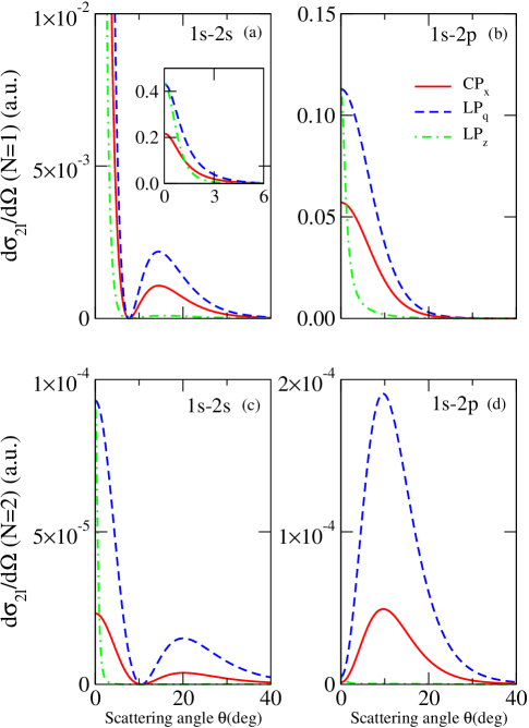
Figure 2: (Color online) Differential cross sections for the laser-assisted inelastic scattering process, $e^{-}$+H($1s$) +$N\omega$ $\to$ $e^{-}$+H($2l$), given by Eq. (27), for $N=1$ in (a) and (b) and $N=2$ in (c) and (d) as a function of the scattering angle $\theta$, with excitation of the $2s$ state in (a) and (c), and $2p$ state in (b) and (d). The full lines represent the scattering geometry CP_x with $\varphi=90^{\circ}$, dashed lines represent the scattering geometry LP_q, and dot-dashed lines represent the scattering geometry LP_z. The initial projectile electron energy is $E_{k_{i}}=200$ eV, the laser field strength is ${\cal E}_{0}=10^{7}$ V/cm, and the photon energy is $2$ eV.

Next, we apply the analytic formulas derived in the above sections to calculate the DCSs for inelastic electron scattering by a hydrogen atom in its ground state in the presence of a CP laser field, and we focus our numerical examples on one- and two-photon absorption. We choose low-photon energies and high energies of the projectile electron, such that neither the photon nor the projectile electron can separately excite an upper atomic state. To start with a simple case we present the angular distributions in Fig. 2 for an initial scattering energy $E_{k_{i}}=200$ eV, a photon energy corresponding to the He:Ne laser $\omega=2$ eV, a laser field strength ${\cal E}_{0}=10^{7}$ V/cm, and an azimuthal angle $\varphi=90^{\circ}$. These laser field parameters correspond to a value of $\alpha_{0}\simeq 0.36$ a.u. and $X_{q}\simeq 0.36|\bm{\varepsilon}\cdot{\mathbf{q}}|$. The DCSs for one- and two-photon absorption ($N=1$ and $2$), calculated from Eq. (27), are plotted as a function of the scattering angle $\theta$ for excitation of the $2s$ state in Figs. 2(a) and 2(c), and of the $2p$ state in Figs. 2(b) and 2(d), in the scattering geometries CP_x (full lines), LP_q (dashed lines), and LP_z (dot-dashed lines). At this laser field strength the two-photon absorption signal is about three-orders of magnitude smaller than the one-photon absorption signal. The DCSs ($1s\to 2s$) for one-photon absorption at small scattering angles [$\theta<6^{\circ}$ in the inset of Fig. 2(a)], show a similar behavior to the DCSs for the elastic scattering process ($1s\to 1s$), as it is shown in Fig. 1(b₂) of Ref. [12]. Very recently there are new experimental detections for Xe of the peak profile at forward scattering angles and a few attempts to explain it based on the Zon’s model [30]. For the $1s\to 2s$ excitation the large values of the scattering signal at $\theta\simeq 0^{\circ}$ can be simple understood from the analytic expression of DCS at low-field intensities, Eq. (44), as arising from the atomic dressing contribution which is proportional to the photon energy, while the projectile contribution is proportional to $q^{2}$ and can be negligible at forward scattering angles.

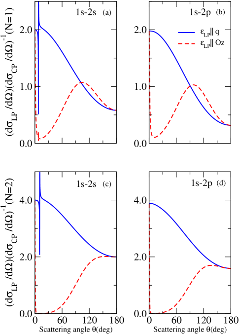
Figure 3: Ratios of the DCSs by the LP and CP fields for $N=1$ in (a) and (b) and $N=2$ in (c) and (d) as a function of the scattering angle $\theta$, with excitation of the $2s$ and $2p$ states. The full lines represent the ratio by the LP_q and CP_x fields, while the dashed line represent the ratio by the LP_z by CP_x fields, with the azimuthal angle $\varphi=90^{\circ}$. The rest of the parameters are the same as in Fig. 2.

Depending of the laser parameters, projectile energies, and scattering geometry the CP scattering signal can be larger or smaller than the LP signal. In order to better understand the differences between the scattering signals by the CP and LP fields plotted in Fig. 2, we compare in Fig. 3 the ratios of the DCSs with excitation of the $2s$ and $2p$ states by the LP and CP fields for $N=1$ in (a) and (b), and $N=2$ in (c) and (d) as a function of the scattering angle $\theta$. In particular, in the domain of non-negligible scattering signal ($\theta<60^{\circ}$) the DCSs for one- and two-photon absorption by the CP_x field are larger than those by the LP_z field and smaller than those by the LP_q field. The ratios of DCSs by the LP and CP fields, $\frac{d{\sigma}_{2l}(\bm{LP}_{q})}{d\Omega}/\frac{d{\sigma}_{2l}(\bm{CP}_{x})}{d\Omega}$ and $\frac{d{\sigma}_{2l}(\bm{LP}_{z})}{d\Omega}/\frac{d{\sigma}_{2l}(\bm{CP}_{x})}{d\Omega}$, as a function of the scattering angle have nearly opposite behavior in Fig. 3, around the value of $1$ for one-photon absorption and $2$ for two-photon absorption. For $1s\to 2s$ excitation at forward scattering angles the CP_x signal for one-photon absorption is one-half of the LP_q signal, as it is displayed in Fig. 3(a) and in the inset windows of Fig. 2(a).

In the perturbative regime ($X_{q}\ll 1$) it can be easily shown from Eq. (43) that the ratio of the one-photon DCSs by the LP_q and CP_x fields is equal to $2$ for the $1s\to 2s$ excitation, because for high projectile energies and low-photon energies, such that $k_{f}\simeq k_{i}$ and $q\simeq 2k_{i}\sin(\theta/2)$, we obtain after simple algebra $\bm{\varepsilon_{{CP}_{x}}}\cdot{\mathbf{q}}\simeq\sqrt{2}k_{i}\sin(\theta/2)$ at $\varphi=90^{\circ}$, that results in a ratio of $|\bm{\varepsilon_{{LP}_{q}}}\cdot{\mathbf{q}}|^{2}/|\bm{\varepsilon_{{CP}_{x}}}\cdot{\mathbf{q}}|^{2}\simeq 2$. At forward scattering angles the CP_x signal is also one-half of the LP_z signal, as it is shown in Fig. 3(a) and in the inset window of Fig. 2(a), because whenever $\theta\simeq 0^{\circ}$ the following ratio holds $|\bm{\varepsilon_{{LP}_{z}}}\cdot{\mathbf{q}}|^{2}/|\bm{\varepsilon_{{CP}_{x}}}\cdot{\mathbf{q}}|^{2}\simeq 2$. The sharp peaks at the scattering angles $7.9^{\circ}$ and $10.7^{\circ}$ in Figs. 3(a) and 3(c) occur due to the dynamic minimum of $1s\to 2s$ excitation DCSs. Similarly, for the $1s\to 2p$ excitation, Figs. 2(b) and 3(b), it can be shown from Eq. (45) derived in the perturbative regime with $X_{q}\ll 1$, that at high projectile energy and low-photon energy the ratio of the one-photon DCSs by the CP_x (with the azimuthal angle $\varphi=90^{\circ}$) and LP_q fields is close to $2$. In the case of two-photon absorption, Figs. 3(c)-3(d), at very small scattering angles $\theta<5^{\circ}$, the CP_x signal is one-quarter of the LP_q signal. For a $N$-photon process in the perturbative regime ($X_{q}\ll 1$), we obtain from Eq. (32) a simple ratio of DCSs in case of $1s\to ns$ excitation

$$\frac{d{\sigma}_{n0}(\bm{LP}_{q})}{d\Omega}\bigg{/}\frac{d{\sigma}_{n0}(\bm{CP}_{x})}{d\Omega}\simeq 2^{|N|},$$ (47)

that is independent of the scattering angle and is similar to the ratio of DCSs by the LP and CP fields for elastic scattering derived in the perturbative domain [12].

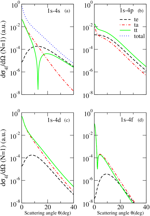
Figure 4: (Color online) Differential cross sections for laser-assisted inelastic scattering process, $e^{-}$+H($1s$)+$\omega$ $\to$ $e^{-}$+H($4l$), given by Eq. (27), with the excitation of the $4l$-subshells ($l=0,1,2$, and $3$) as a function of the scattering angle $\theta$ for the (a) $1s\to 4s$, (b) $1s\to 4p$, (c) $1s\to 4d$, and (d) $1s\to 4f$ transitions. The dashed lines represent the projectile electron contribution, while the dot-dashed lines represent the atomic contribution to DCS. The scattering geometry is CP_x with $\varphi=90^{\circ}$ and the laser parameters are the same as in Fig. 2.

Figures 4(a)-4(d) show the angular distributions for one-photon absorption ($N=1$), calculated from Eq. (27) in a logarithmic scale, corresponding to the (a) $1s\to 4s$, (b) $1s\to 4p$, (c) $1s\to 4d$, and (d) $1s\to 4f$ excitations of hydrogen in the scattering geometry CP_x with the azimuthal angle $\varphi=90^{\circ}$. The incident projectile energy and laser parameters are the same as in Fig. 2. The dashed lines correspond to DCSs which neglect the atomic dressing given by Eq. (33) and the dot-dashed lines represent the atomic contribution to the DCS calculated as ${(2\pi)}^{4}{k_{f}}/{k_{i}}\sum_{m=-l}^{l}{|T_{nlm}^{(1)}(N=1)|}^{2}$. The total inelastic DCS for the excitation of the $n=4$ level is shown by the dotted line in Fig. 4(a). The atomic dressing effects are dominant at small scattering angles for the excitation of the $4l$-subshells ($l=0,1,2$, and $3$), as well at large scattering angles for the excitation of the $4d$ and $4f$ states only. Dynamic minimum of DCS in Fig. 4(a), which is independent of the scattering geometry and represents the result of cancellation of the electronic and atomic radial integrals in Eq. (27), occurs for the $1s\to 4s$ excitation only at the scattering angle $\theta\simeq 12.6^{\circ}$.

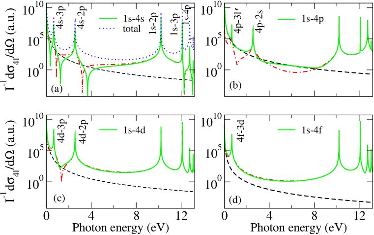
Figure 5: (Color online) Differential cross sections for laser-assisted inelastic scattering process, $e^{-}$+H($1s$)+$\omega$ $\to$ $e^{-}$+H($4l$), given by Eq. (39), with the excitation of the $4l$-subshells ($l=0,1,2$, and $3$) as a function of the laser photon energy $\omega$, at the projectile electron energy of $E_{k_{i}}=500$ eV and the scattering angle of $5^{\circ}$, for the (a) $1s\to 4s$, (b) $1s\to 4p$, (c) $1s\to 4d$, and (d) $1s\to 4f$ transitions. The dashed lines represent the projectile electron contribution, while the dot-dashed lines represent the atomic contribution to DCS. The dotted line in Fig. 5(a) represents the total DCS for the excitation of the $n=4$ level. The scattering geometry is CP_x with $\varphi=90^{\circ}$ and the DCSs are normalized by the laser intensity $I$.

At low laser intensities we show in Figs 5(a)-5(d) the DCSs, given by Eq. (39), with respect to the laser photon energy for one-photon absorption ($N=1$) corresponding to the (a) $1s\to 4s$, (b) $1s\to 4p$, (c) $1s\to 4d$, and (d) $1s\to 4f$ excitations of hydrogen in the scattering geometry CP_x. The DCSs are normalized to the laser intensity and calculated at a higher incident projectile electron energy $E_{k_{i}}=500$ eV, a scattering angle $\theta=5^{\circ}$, and an azimuthal angle $\varphi=90^{\circ}$. The dashed lines correspond to DCSs which neglect the atomic dressing given by Eq. (42) and the dot-dashed lines represent the atomic contribution to the DCS. The total inelastic DCS for the excitation of the $n=4$ level is plotted by the dotted line in Fig. 5(a). The DCSs for $1s\to 4l$ ($l=0,1,2$, and $3$) excitations as a function of the photon energy show a strongly dependence on the atomic structure and exhibits two sets of resonances. These two sets of resonances generally occur, as schematically plotted in Fig. 6, due to the simultaneous projectile electron-photon excitation of hydrogen to the $4l$ state either (i) by first absorbing some of the projectile electron kinetic energy, then absorbing (emitting) a photon from (to) the laser field or (ii) by first absorbing a photon from the laser field, then absorbing (transferring) the energy difference from (to) the projectile electron. The first set of resonances in Figs. 5(a)-5(d) occurs at the photon energy $\omega\simeq 0.66$ eV, that matches the energy difference between the $4s$ and $3p$ states. The origin of this resonance resides in the dipole coupling of a final $4l$ state and a lower intermediate $3l^{\prime}$ state ($l^{\prime}=l\pm 1$ with $l^{\prime}<3$). The second resonance with a similar origin occurs at $\omega\simeq 2.55$ eV in Figs. 5(a)-5(c) due to the dipole coupling of a final $4l$ state and a lower intermediate $2l^{\prime}$ state ($l^{\prime}=l\pm 1$ with $l^{\prime}<2$). As it can be noted from Eq. (20) this first set of resonances is related to the poles of the atomic transition amplitude due to the atomic radial integral ${\cal J}^{b}_{4ll^{\prime},1s}(\Omega_{4}^{-},q)$, given by Eq. (57), at photon energies such that $\omega_{4n^{\prime}}=(1/{n^{\prime}}^{2}-1/4^{2})/2$, with $n^{\prime}=2$ and $3$. The second set of resonances that appear in Figs. 5(a)-5(d), at photon energies $\omega\simeq 10.2,12.09,12.75$ eV,…, are associated to the $1s\to n^{\prime}p$ atomic transitions ($n^{\prime}=2,3,4,...$). These resonances occur due to one-photon absorption from the initial $1s$ state to an intermediate $n^{\prime}p$ state, followed by a transition to the final $4l$ state by projectile electron interaction, as it can be understood from the atomic transition amplitude Eq. (19) and Fig. 6(ii). For this second set of resonances the other atomic radial integral ${\cal J}^{a}_{4ll^{\prime},1s}(\Omega_{1}^{+},q)$, given by Eq. (55), presents poles that occur at photon energies that match atomic resonances such that $\omega_{n^{\prime}1}=(1-1/{n^{\prime}}^{2})/2$, with $n^{\prime}\geq 2$. We remark that, despite the new experimental progresses on laser-assisted electron-atom scattering [29, 28], such investigations are still quite difficult to accomplish, especially for those involving excited states of atoms. From the experimental point of view we believe that some of these resonances are particularly interesting [31], and it may be feasible to detect the inelastic process at photon energies close to the $0.66$- or $2.55$-eV resonances because these values do not correspond to any resonance of the elastic scattering processes of hydrogen from its ground state [45].

4 Summary and conclusions

In this paper study the influence of laser polarization in electron-impact excitation of hydrogen atoms in a circularly polarized laser field. Using a semi-perturbative method new analytic formulas in a closed form have been derived for the DCSs in laser-assisted inelastic electron-hydrogen scattering for $1s\to nl$ excitation, which are valid for both linear and circular polarization, with the kinematic part that depends on the scattering geometry and photon polarization vector clearly separated. We obtained a very good agreement with the earlier numerical results for LP fields, showing the accuracy and efficiency of our theoretical results. A comparison between the linear and circular polarizations of the laser field was made for different scattering geometries for the excitation of the $n=2$ levels and important differences occur between the scattered electron angular distributions depending on the type of polarization: CP_x, LP_q, and LP_z. From the extensive calculations we have obtained that, at non-resonant photon energies in the domain of non-negligible scattering signal (at scattering angles $\theta<60^{\circ}$), the DCSs for one- and two-photon excitation of the $2s$ and $2p$ states by the CP_x field are generally larger than by the LP_z field, and smaller than by the LP_q field. The detailed numerical data presented for the excitation of the $n=4$ levels by CP fields indicate that the atomic dressing effects for inelastic processes are important and we found a significant increase in the DCSs at small scattering angles for the $s-s$, $s-d$, and $s-f$ optically forbidden transitions due to the simultaneous electron-photon excitation. We have also elucidated the origin of the peaks in the resonance structure of DCSs as occurring due to the dipole coupling of the initial ground state with $n^{\prime}p$ states and of the final excited state with $n^{\prime}l^{\prime}$ ($l^{\prime}=l\pm 1$) states. It was found that by changing the laser field polarization the angular distribution and the photon frequency dependence of the scattering signal can be modified.

Appendix A Analytic expression for the electric radial integral ${\cal I}_{nl}$

We recall that the electronic radial integral, ${\cal I}_{nl}$, needed for the calculation of the inelastic electronic transition amplitude, $T_{nlm}^{(0)}$, is defined as

$${\cal I}_{nl}(q)={\int}_{0}^{\infty}dr\ r^{2}R_{nl}(r)j_{l}(qr)R_{10}(r)-\delta_{n1}\delta_{l0}.$$ (48)

Different methods can be used for the calculation of the electronic radial integral [47], and an analytic expression for the electronic radial integral is obtained, after performing the integration over the projectile coordinates, as a finite sum of Gauss hypergeometric function, ${}_{2}F_{1}$:

$${\cal I}_{nl}(q) = \frac{1}{q}\frac{2^{l+2}}{(2l+1)!}\left[\frac{(n+l)!}{(n-l-1)!}\right]^{1/2}$$ (49)

$$\times{\rm Re}\left\{\sum_{p=0}^{l}\frac{i^{p-l-1}}{(2q)^{p}}\frac{(l+p)!}{p!(l-p)!}\frac{(l+1-p)!}{(1+n-iqn)^{2+l-p}\;n^{p}}\right.$$

$$\times\left.{}_{2}F_{1}(l+2-p,l-n+1,2l+2,\frac{2}{1+n-iqn})\right\}-\delta_{n1}\delta_{l0}.$$

For the particular case of $1s\to 2s$ excitation, the electronic integral ${\cal I}_{20}$ calculated from Eq. (49) is given by

$${\cal I}_{20}(q)=\frac{4\sqrt{2}\;q^{2}}{(9/4+q^{2})^{3}}\;,$$ (50)

while for the $1s\to 2p$ excitation, the electronic radial integral ${\cal I}_{21}$ reads

$${\cal I}_{21}(q)=\frac{2\sqrt{6}\;q}{(9/4+q^{2})^{3}}\;,$$ (51)

where the expressions of ${\cal I}_{20}$ and ${\cal I}_{21}$ agree with the formulas given by Bransden and Joachain [43].

Appendix B Analytic expressions for the atomic radial integrals ${\cal J}^{a}_{nll^{\prime},1s}$ and ${\cal J}^{b}_{nll^{\prime},1s}$

In order to evaluate the atomic transition amplitude $T_{nlm}^{(1)}$ the atomic radial integral ${\cal J}_{nll^{\prime}}$, Eq. (25), is rewritten as the difference between two atomic radial integrals,

$${\cal J}_{nll^{\prime}}({\pm}\omega,q)\equiv{\cal J}_{nll^{\prime}}(\tau_{1}^{\mp},\tau_{n}^{\pm},q)={\cal J}_{nll^{\prime},1s}^{a}(\tau_{1}^{\mp},q)-{\cal J}_{nll^{\prime},1s}^{b}(\tau_{n}^{\pm},q)\;,$$ (52)

with the selection rule $l^{\prime}=l\pm 1$, where the dependence of the atomic radial integrals on the energies $\Omega$ is now included in the new parameters $\tau^{+}_{n}=1/\sqrt{-{2\Omega^{-}_{n}}}$ and $\tau^{-}_{n}=1/\sqrt{-{2\Omega^{+}_{n}}}$. The two radial integrals on the right-hand side of Eq. (52) are defined as,

$${\cal J}_{nll^{\prime},1s}^{a}(\tau_{1},q)={\int}_{0}^{\infty}dr\ r^{2}R_{nl}(r)j_{l^{\prime}}(qr){\cal B}_{101}(\tau_{1};r)\;,$$ (53)

and

$${\cal J}_{nll^{\prime},1s}^{b}(\tau_{n},q)={\int}_{0}^{\infty}dr\ r^{2}R_{10}(r)j_{l^{\prime}}(qr){\cal B}_{nll^{\prime}}(\tau_{n};r)\;,$$ (54)

where the radial functions ${\cal B}_{nll^{\prime}}(\tau;r)$ are defined in Ref. [36].

By using the development of the spherical Bessel function in Eq. (53), after performing some calculations, we obtained an analytically expression for the atomic radial integral ${\cal J}_{nll^{\prime},1s}^{a}$ in terms of finite sums of the Appell hypergeometric functions [48], $F_{1}$, of two variables,

$${\cal J}_{nll^{\prime},1s}^{a}(\tau,q) = \frac{2^{\tau+l+4}\;\tau}{q\;n^{2+l}(1+\tau)^{2+\tau}(1-\tau)^{2}(2-\tau)}\frac{1}{(2l+1)!}\left[\frac{(n+l)!}{(n-l-1)!}\right]^{1/2}$$ (55)

$$\times{\rm Re}\left\{\sum_{p=0}^{l^{\prime}}\frac{i^{p-l^{\prime}-1}}{(2q)^{p}}\frac{(l^{\prime}+p)!}{p!(l^{\prime}-p)!}\sum_{s=0}^{n-l-1}\frac{(l+1-n)_{s}}{(2l+2)_{s}s!}\left(\frac{2}{n}\right)^{s}\right.$$

$$\times(2+l-p+s)!\left(\frac{n\tau}{n+\tau-iqn\tau}\right)^{3+l-p+s}$$

$$\times\left.F_{1}(2-\tau,-1-\tau,3+l-p+s,3-\tau,x_{1},y_{1})\right\}.$$

The term $(p)_{s}$, with $p$ and $s$ integers, denotes the Pochhammer’s symbol and the Appell hypergeometric functions $F_{1}$ depend on the variables

$$x_{1}=\frac{1-\tau}{2},\;y_{1}=\frac{n(1-\tau)}{n+\tau-iqn\tau}\;.$$ (56)

Note that ${\cal J}_{nll^{\prime},1s}^{a}$, Eq. (55), presents poles with respect to $\tau$ which arise due to the cancellation of the $n^{\prime}-\tau$ ($n^{\prime}=1,2$) denominators and from the poles of the Appell hypergeometric functions for $\tau=n^{\prime}$, where $n^{\prime}$ is an integer ($n^{\prime}>2$). The origin of these poles resides in the poles of the Coulomb Green’s functions employed for the calculation of $\textbf{w}_{nlm}$ vectors [36]. The second set of one-photon resonances discussed in Figs. 5(a)-5(d) is related to the poles of the radial integral ${\cal J}_{nll^{\prime},1s}^{a}(\tau_{1}^{\pm},q)$ at at $\tau_{1}^{-}=n^{\prime}$ with $n^{\prime}>1$.

We consider now the other atomic radial integral ${\cal J}_{nll^{\prime},1s}^{b}$ defined in Eq. (54) which is calculated, in the same manner as ${\cal J}_{nll^{\prime},1s}^{a}$, in terms of finite sums of Appell hypergeometric functions, $F_{1}$, as

$${\cal J}_{nll^{\prime},1s}^{b}(\tau,q) = \frac{\tau}{q}\;\frac{2^{2l^{\prime}+\tau+2}\;n^{\tau-1}}{(2l^{\prime}+1)!}\left[\frac{(n+l)!}{(n-l-1)!}\right]^{1/2}{\rm Re}\left\{\sum_{k=-1,1}d_{\;n,l}^{\;l^{\prime},-k}\right.$$ (57)

$$\times\sum_{p=0}^{l^{\prime}}\frac{i^{p-l^{\prime}-1}}{(2q)^{p}}\frac{(l^{\prime}+p)!}{p!(l^{\prime}-p)!}\sum_{\nu=0}^{n-l^{\prime}-1-k}\frac{(4)^{\nu}}{\nu!}(l^{\prime}+1-p+\nu)!$$

$$\times\sum_{\mu=0}^{n-l^{\prime}-1-k-\nu}\left(\frac{-1}{2n}\right)^{\mu}\frac{(l^{\prime}+1+k-n)_{\mu+\nu}}{b\;(2l^{\prime}+2)_{\nu}\mu!}$$

$$\times\frac{(n+\tau)^{k+2\mu-n-\tau}}{(n-\tau)^{k+\mu+\nu-n+l^{\prime}+1}}\left(\frac{\tau}{1+\tau-iq\tau}\right)^{2+l^{\prime}-p+\nu}$$

$$\times\left.F_{1}(b,-n-\tau+1+k+\mu,2+l^{\prime}-p+\nu,b+1,x_{n},y_{n})\right\},$$

where the expressions $d_{\;n,l}^{\;l+1,1}=(n+l+1)(n+l+2)$, $d_{\;n,l}^{\;l-1,1}=1$, and $d_{\;n,l}^{\;l^{\prime},-1}=-d_{-n,l}^{\ l^{\prime},1}$ are defined in [36], $b=l^{\prime}+1-\tau+\mu+\nu$, and the Appell hypergeometric functions $F_{1}$ depend on other two variables

$$x_{n}=\frac{n-\tau}{2n},\;y_{n}=\frac{n-\tau}{n(1+\tau-iq\tau)}.$$ (58)

Compared to ${\cal J}^{a}_{nll^{\prime},1s}$, the atomic radial integral ${\cal J}^{b}_{nll^{\prime},1s}$ presents poles with respect to $\tau$ in Eq. (57), which arise due to the cancellation of the $n-\tau$ and $b$ denominators, as well as from the poles of the Appell hypergeometric function $F_{1}$ for $\tau=n^{\prime}$, where $n^{\prime}$ is an integer. The first set of one-photon resonances discussed in Figs. 5(a)-5(d) is related to the poles of the radial integral ${\cal J}_{nll^{\prime},1s}^{b}(\tau_{n}^{\pm},q)$ at $\tau_{n}^{-}=n^{\prime}$ with $n^{\prime}>n$ (for emission) and $\tau_{n}^{+}=n^{\prime}$ with $n^{\prime}<n$ (for absorption).

In addition, for the $1s\to 2s$ excitation the atomic radial integral ${\cal J}_{201}(\omega,q)$ calculated from Eqs. (52), (55), and (57) is approximated in the low-photon energy limit ($\omega\ll E_{n}-E_{1s}$) as

$${\cal J}_{201}(\omega,q)\simeq-q\frac{18\sqrt{2}}{(9/4+q^{2})^{3}}+q\;\omega\frac{3\sqrt{2}(243+684q^{2}+128q^{4})}{2(9/4+q^{2})^{5}},$$ (59)

while for the $1s\to 2p$ excitation we obtain simple formulas in the low-photon energy limit of ${\cal J}_{210}(\omega,q)$ and ${\cal J}_{212}(\omega,q)$

$${\cal J}_{210}(\omega,q) \simeq -{q^{2}}\frac{12\sqrt{6}}{(9/4+q^{2})^{3}}-q\;\omega\frac{\sqrt{6}(1701+3780q^{2}-336q^{4}-64q^{6})}{16(9/4+q^{2})^{5}},$$ (60)

$${\cal J}_{212}(\omega,q) \simeq q^{2}\omega\frac{18\sqrt{6}(21+4q^{2})}{(9/4+q^{2})^{5}},$$ (61)

where the neglected terms are of $\omega^{2}$ order. These asymptotic expressions are very useful to provide simple approximate formulas for $1s\to 2s$ and $1s\to 2p$ excitation DCSs, Eqs. (44) and (46), and to verify the numerical results from Eqs. (43) and (45), as well.

Appendix C Some useful summation formulas for the vector spherical harmonics, $\textbf{V}_{l^{\prime}lm}$

The well-known summation formulas of the vector spherical harmonics [37], $\mathbf{V}_{l\pm 1lm}$, used for the calculation of the DCS, Eq. (27), and of the quantities $B_{nl}$, Eq. (29), $C_{nl}$, Eq. (30), and $D_{nl}$, Eq. (31), are presented below:

$$\sum_{m=-l}^{l}[\textbf{a}_{1}\cdot\textbf{V}_{l+1lm}^{*}(\hat{\textbf{q}})][\textbf{a}_{2}\cdot\textbf{V}_{l+1lm}(\hat{\textbf{q}})] = \frac{1}{8\pi}\left[l\textbf{a}_{1}\cdot\textbf{a}_{2}+(l+2)(\textbf{a}_{1}\cdot\hat{\textbf{q}})(\textbf{a}_{2}\cdot\hat{\textbf{q}})\right],$$ (62)

$$\sum_{m=-l}^{l}[\textbf{a}_{1}\cdot\textbf{V}_{l-1lm}^{*}(\hat{\textbf{q}})][\textbf{a}_{2}\cdot\textbf{V}_{l-1lm}(\hat{\textbf{q}})] = \frac{1}{8\pi}\left[(l+1)\textbf{a}_{1}\cdot\textbf{a}_{2}+(l-1)(\textbf{a}_{1}\cdot\hat{\textbf{q}})(\textbf{a}_{2}\cdot\hat{\textbf{q}})\right],$$ (63)

$$\sum_{m=-l}^{l}[\textbf{a}_{1}\cdot\textbf{V}_{l+1lm}^{*}(\hat{\textbf{q}})][\textbf{a}_{2}\cdot\textbf{V}_{l-1lm}(\hat{\textbf{q}})] = \frac{\sqrt{l(l+1)}}{8\pi}\left[\textbf{a}_{1}\cdot\textbf{a}_{2}-3(\textbf{a}_{1}\cdot\hat{\textbf{q}})(\textbf{a}_{2}\cdot\hat{\textbf{q}})\right],$$ (64)

$$\sum_{m=-l}^{l}Y^{*}_{lm}(\hat{\textbf{q}})\textbf{V}_{l+1lm}(\hat{\textbf{q}}) = -\frac{\sqrt{(l+1)(2l+1)}}{4\pi}\;\;\hat{\textbf{q}},$$ (65)

$$\sum_{m=-l}^{l}Y^{*}_{lm}(\hat{\textbf{q}})\textbf{V}_{l-1lm}(\hat{\textbf{q}}) = \frac{\sqrt{l(2l+1)}}{4\pi}\;\hat{\textbf{q}}.$$ (66)

Figure 1: The specific scattering geometries assumed for the numerical calculations of laser-assisted $e^{-}$-H($1s$) scattering. $\mathbf{k}_{i}$ and $\mathbf{k}_{f}$ are the initial and final momentum vectors of the projectile electron, $\theta$ is the angle between them, and $\mathbf{q}$ is the momentum transfer vector. $\mathbf{k}$ is the wave vector of the photon, $\bm{\varepsilon}$ represents the polarization vector of the laser field, and $\varphi$ is the azimuthal angle. We consider the scattering geometries with $\mathbf{k}_{i}\parallel Oz$ and the field polarizations denoted as (a) CP_x where the laser field is circularly polarized, $\bm{\varepsilon_{{CP}_{x}}}$ lies in the $yz$ plane, and the laser field propagates along the $x$-axis, (b) LP_q where the laser field is linearly polarized $\bm{\varepsilon_{{LP}_{q}}}\parallel\mathbf{q}$, and (c) LP_z where the laser field is linearly polarized $\bm{\varepsilon_{{LP}_{z}}}\parallel Oz$.

Figure 6: (Color online) Schematic energy level diagrams relevant for the simultaneously projectile electron-photon excitation of hydrogen to an $nl$ ($n>2$) state either (i) by first absorbing some of the projectile electron kinetic energy, then absorbing (emitting) a photon from (to) the laser field or (ii) by first absorbing a photon from the laser field, then absorbing (transferring) the energy difference from (to) the projectile electron.

References

• [1] Cohen-Tannoudji C, Dupont-Roc J, Grynberg G. Atom-photon Interactions: basic processes and applications. New York: Wiley-VCH; 1992.
• [2] Shima Y, Yatom H. Inverse bremsstrahlung energy absorption rate. Phys Rev A 1975;12:2106-117; Lima MBS, Lima CAS, Miranda LCM. Screening effect on the plasma heating by inverse bremsstrahlung. Phys Rev A 1979;19:1796-800.
• [3] Chandrasekhar S. An Introduction to the Study of Stellar Structure. Mineola, NY: Dover; 1967. p. 249-91; Seaton MJ. In: Bederson B, Dalgarno A, editors. Advances in Atomic, Molecular and Optical Physics. New York: Academic Press; 1994.
• [4] Mott NF, Massey HSW. The Theory of Atomic Collisions. London: Oxford University Press; 1965. Joachain C. Quantum Collision Theory. Amsterdam: North Holland; 1987.
• [5] Mason NJ. Laser-assisted electron-atom collisions. Rep Prog Phys 1993;56:1275-346.
• [6] Ehlotzky F, Jaroń A, Kamiński JZ. Electron-atom collisions in a laser field. Phys Rep 1998;297:63-153.
• [7] Ehlotzky F. Atomic phenomena in bichromatic laser fields. Phys Rep 2001;345:175-264.
• [8] Bransden BH, Joachain CJ. Physics of Atoms and Molecules. London: Longman; 1983.
• [9] Joachain CJ, Kylstra NJ, Potvliege RM. Atoms in Intense Laser Fields. Cambridge, UK: Cambridge University Press; 2012. p. 466-549.
• [10] Fainstein PD, Maquet A. Polarization dependence of laser-assisted electron-atom elastic collisions. J Phys B: At Mol Phys 1994;27:5563-71.
• [11] Cionga A, Buică G. Polarization Effects in Two-Photon Free-Free Transitions in Laser-Assisted Electron-Hydrogen Collisions. Laser Phys 1998;8:164-71.
• [12] Cionga A, Ehlotzky F, Zloh G. Electron-atom scattering in a circularly polarized laser field. Phys Rev A 2000;61:063417-1-11.
• [13] Cionga A, Ehlotzky F, Zloh G. Circular dichroism in free-free transitions of high-energy electron-atom scattering. Phys Rev A 2000;62:063406-1-5; Dichroism in high energy electron-hydrogen scattering in an elliptically polarized laser field. Opt Commun 2001;192:255-62.
• [14] Bouzidi M, Makhoute A, Hounkonnou MN. Polarization effect of laser field in inelastic electron-hydrogen collisions. Eur Phys J D 1999;5:159-65; Akramine O El, Makhoute A, Khalil D, Maquet A, Taïeb R. Effects of laser polarization in laser-assisted electron-helium inelastic collisions: a Sturmian approach J Phys B 1999;32:2783-99.
• [15] Radzig AA, Smirnov BM. Reference Data on Atoms, Molecules, and Ions. Berlin: Springer; 1985. p. 87-120.
• [16] Milosevic DB, Ehlotzky F, Piraux B. Inelastic electron-atom collisions in a bichromatic laser field. J Phys B 1997;30:4347-61.
• [17] Cionga A, Ehlotzky F, Zloh G. Elastic electron scattering by excited hydrogen atoms in a laser field. Phys Rev A 2001;64:043401-1-10.
• [18] Buica G. Inelastic scattering of electrons by metastable hydrogen atoms in a laser field. Phys Rev A 2015;92:033421-1-11.
• [19] Jetzke S, Broad S, Maquet A. Electron-hydrogen collisions in the presence of a laser field: one-photon excitation. J Phys B: At Mol Phys 1987;20:2887-97.
• [20] Francken P, Attaourti Y, Joachain CJ. Laser-assisted inelastic electron-atom collisions. Phys Rev A 1998;38:1785-96.
• [21] Bhattacharya M, Sinha C, Sil NC. Excitation of the hydrogen atom by fast-electron impact in the presence of a laser field. Phys Rev A 1991;44:1884-97.
• [22] Cionga A, Florescu V. One-photon excitation in the e-H collision in the presence of a laser field. Phys Rev A 1992;45:5282-85.
• [23] Vučić S. Inelastic fast-electron-hydrogen-atom collision in a laser field. Phys Rev A 1995;51:4754-61.
• [24] Voitkiv AB, Najjari B, Ullrich J. Inelastic Collisions of Relativistic Electrons with Atomic Targets in a Laser Field. Phys Rev Lett 2009;103:193201-1-4.
• [25] Mason NJ, Newell WR. Simultaneous electron-photon excitation of the helium $2^{3}$S state. J Phys B: At Mol Opt Phys 1989;22:777-96.
• [26] Mason NJ, Newell WR. The polarisation dependence of the simultaneous electron-photon excitation cross section of the helium $2^{3}$S state. J Phys B: At Mol Opt Phys 1990;23:L179-82.
• [27] Musa MO, MacDonald A, Tidswell L, Holmes J, Wallbank B. Laser-induced free-free transitions in elastic electron scattering from CO2. J Phys B: At Mol Phys 2010;43:175201-1-10.
• [28] Kanya R, Morimoto Y, Yamanouchi K. Observation of Laser-Assisted Electron-Atom Scattering in Femtosecond Intense Laser Fields. Phys Rev Lett 2010;105:123202-1-4.
• [29] de Harak BA, Ladino L, MacAdam KB, Martin NLS. High-energy electron-helium scattering in a Nd:YAG laser field. Phys Rev A 2011;83:022706-1-6.
• [30] Morimoto Y, Kanya R, Yamanouchi K. Light-Dressing Effect in Laser-Assisted Elastic Electron Scattering by Xe. Phys Rev Lett 2015;115:123201-1-5; Kanya R, Morimoto Y, Yamanouchi K. Progress in Ultrafast Intense Laser Science. In: Yamanouchi K, Paulus G, Mathur D, editors. Switzerland: Springer International Publishing; 2014. p. 1-16.
• [31] Dunseath KM, Terao-Dunseath M. Simultaneous electron-photon excitation of helium in a CO2 laser field. J Phys B: At Mol Phys 2011;44:135203-1-11; Simultaneous electron-photon excitation of helium in an Nd:YAG laser field. J Phys B: At Mol Phys 2013;46:235201-1-10.
• [32] Ajana I, Makhoute A, Khalil D. Low-energy electron-helium scattering in a Nd–YAG laser field. J Electron Spectrosc Relat Phenom 2014;192:19-25.
• [33] Byron Jr FW, Joachain CJ. Electron-atom collisions in a strong laser field. J Phys B 1984;17:L295-301.
• [34] Makhoute A, Khalil D, Zitane M, Bouzidi M. The second Born approximation in electron-atom collisions in the presence of a laser field. J Phys B 2002;35:957-72.
• [35] Volkov DM. On a class of solutions of the Dirac equation. Z Phys 1935;94:250-60.
• [36] Florescu V, Marian T. First-order perturbed wave functions for the hydrogen atom in a harmonic uniform external electric field. Phys Rev A 1986;34:4641-6.
• [37] Varshalovich DA, Moskalev AN, Hersonski VK. Kvantoivaia Teoria Uglovogo Momenta. Leningrad: Nauka; 1975.
• [38] Watson GN. Theory of Bessel Functions. Cambridge, UK: Cambridge University Press; 1962.
• [39] Bunkin FV, Fedorov MV. Bremsstrahlung in a strong radiation field. Sov Phys JETP 1966;22:844-7.
• [40] Kroll NM, Watson KM. Charged-particle scattering in the presence of a strong electromagnetic wave. Phys Rev A 1973;8:804-9.
• [41] Cavaliere P, Leone C. Inelastic scattering of a charged particle by hydrogenic atoms. Nuovo Cim 1979;49:512-24.
• [42] Beigman IL, Chichkov BN. Subthreshold excitation of atoms by electrons in an intense optical field. JETP Lett 1987;46;395-8.
• [43] Bransden BH, Joachain CJ. Quantum Mechanics. Harlow: Pearson Education Limited; 2000.
• [44] Kracke G, Briggs JS, Dubois A, Maquet A, V. Veniard V. Two-photon free-free transitions in laser-assisted electron-hydrogen scattering. J Phys B 1994;27:3241-56.
• [45] Dubois A, Maquet A, Jetzke S. Electron-H-atom collisions in the presence of a laser field: One-photon free-free transitions. Phys Rev A 1986;34:1888-95.
• [46] Dubois A, Maquet A. Bremsstrahlung radiation emitted in fast-electron-H-atom collisions. Phys Rev A 1989;40:4288-97.
• [47] Whelan C. On the calculation of cross-sections for electron neutral atom collisions in the Born approximation to the reactance matrix. Math Proc Camb Philos Soc 1984;95:179-86.
• [48] Appell P, Kampé de Fériet P. Fonctions Hypergéométriques et Hypersphériques. Polynomes d’Hermite. Paris: Gauthier-Villars; 1926.
Refer to caption
Refer to caption
Refer to caption