The Universal Law of Generalization Holds for Naturalistic Stimuli

Abstract

Shepard’s universal law of generalization is a remarkable hypothesis about how intelligent organisms should perceive similarity. In its broadest form, the universal law states that the level of perceived similarity between a pair of stimuli should decay as a concave function of their distance when embedded in an appropriate psychological space. While extensively studied, evidence in support of the universal law has relied on low-dimensional stimuli and small stimulus sets that are very different from their real-world counterparts. This is largely because pairwise comparisons – as required for similarity judgments – scale quadratically in the number of stimuli. We provide direct evidence for the universal law in a naturalistic high-dimensional regime by analyzing an existing dataset of $214,200$ human similarity judgments and a newly collected dataset of $390,819$ human generalization judgments ($N=2406$ US participants) across three sets of natural images.

1 Statement of Relevance

Humans constantly form generalizations, whether when trying to identify the color of an object or reasoning about which action to take based on past experiences. Understanding how generalizations relate to underlying psychological representations is a core problem in cognitive science. The universal law of generalization is a fundamental hypothesis concerning the nature of this relationship which states that the strength of generalization between two stimuli should decay as a universal exponential function of their psychological distance. While extensively studied, evidence for the universal law comes from small datasets and artificial stimuli that are very different from the real world. Our work is the first to provide direct evidence for the universal law in a high-dimensional naturalistic domain by collecting and analyzing $605,019$ human similarity and generalization judgments for natural images.

Every day, humans interact with complex perceptual objects that vary in modality, structure and function. Whether deciding when to cross a street, recognizing the face of a friend, or trying to determine whether a novel fruit will taste good, we need to form meaningful generalizations from past perceptual experiences. This problem of generalization is arguably one that we share with all intelligent species, something that led Roger Shepard to propose a candidate for the first universal law of psychology [29]. Shepard’s universal law of generalization – intended to hold for intelligent entities anywhere in the universe – asserts that the extent to which a property is generalized from one stimulus to another should decrease as a concave function (usually exponential) of the distance between those stimuli in psychological space. This idea has been elaborated upon in Bayesian models of cognition [32], and linked to information-theoretic principles such as maximum entropy [16], Kolmogorov complexity [4], and efficient coding [30].

Implicit in Shepard’s proposal is the idea that it is possible to represent perceptual stimuli in a psychological space – typically a low-dimensional representation where the similarity between two stimuli decreases with their distance. While this idea is controversial (e.g., [33]; [34]; [19]), Shepard showed that such spaces can capture the similarity relationships between a variety of simple perceptual stimuli. He proposed a procedure, known as multidimensional scaling (MDS), for uncovering the structure of mental representations from behavioral data ([27]; [28]; [31]). Given a set of stimuli, the procedure begins by constructing a similarity matrix between all stimulus pairs, e.g., by collecting similarity judgments or confusion probabilities, and then applying an iterative algorithm that embeds those stimuli in a psychological space (typically Euclidean) such that similar stimuli are mapped to nearby points.

Having mapped stimuli to points in a psychological space, it becomes possible to test the universal law. While Shepard’s (non-metric) multidimensional scaling method assumes similarity decreases with distance, it doesn’t specify the form of that function. By analyzing the abstract question of how an ideal organism should decide whether two stimuli shared a given property, [29] showed that this function should be concave. Mathematical analysis of a variety of different assumptions about the distribution of properties in psychological space showed that generalization typically decreased as an exponential function of distance. Shepard then demonstrated that this theoretical relationship held for a wide array of stimuli that had been embedded into a psychological space via MDS, including geometric shapes, phonemes, colors (in both humans and pigeons), and even Morse code signals.

Despite the success of Shepard’s account, two clear limitations remain. First, for a set of $N$ stimuli MDS requires on the order of $N^{2}$ pairwise comparisons to construct a full similarity matrix which, as the number of stimuli increases, necessitates a large amount of human data. For example, a set of 100 stimuli would require on the order of 10,000 similarity judgments, without even including any repetitions to ensure data quality. This bottleneck has recently propelled a line of research aimed at finding cheaper approximations for human similarity matrices ([24]; [11]; [15]). Second, and in part as a result of the first limitation, most of the evidence for the universal law comes from studies that are limited to low-dimensional artificial stimuli and small stimulus sets ([29]; [5]; [7]; [30]). Even though more recent work such that of [30] has considered somewhat richer stimuli such as synthesized instrument timbres and vibrotactile patterns, these were still limited to small datasets on the scale of 10-20 stimuli. These limitations make it hard to draw conclusions about the status of the universal law of generalization in the high-dimensional regime of real-world stimuli, especially as fundamental problems in psychology continue to be reshaped by large-scale behavioral studies (see e.g., [1]; [2]; [21]; [14]).

To address this gap, we leveraged recent advances in online recruitment as well as the availability of naturalistic image datasets to directly test the universal law of generalization in a high-dimensional setting. Specifically, we considered a dataset of similarity judgments over three sets of images recently collected by [20] where each dataset comprised 120 images from a given natural category, namely, animals, fruits, and vegetables. This dataset consisted of 214,200 human judgments. To account for the different ways in which similarity scores can be constructed, we augmented this dataset with a newly collected set of generalization judgments where participants rated how likely it is a certain blank property ([17]; [12]) (e.g., having an enzyme) generalizes from one stimulus to another. The latter dataset comprises $390,819$ generalization judgments from $2,406$ online participants. We used these data to directly test the universal law of generalization in this high-dimensional large-scale regime.

All data and analysis code considered in the present work, as well as all necessary code for reproducing the online behavioral experiments are made publicly available in the following OSF repository: https://tinyurl.com/tmwu6pxv. All participants provided informed consent prior to participation in accordance with an approved Princeton University Institutional Review Board (IRB) protocol (#10859).

2 Methods

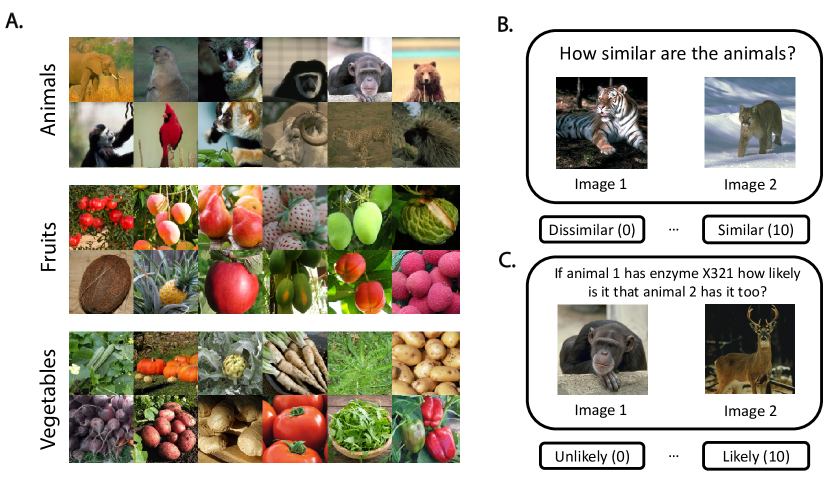
Figure 1: Example images from three natural categories, namely, animals, fruits, and vegetables (A), and schematics of the two elicitation queries used in the present work, namely, direct similarity judgments (B), and generalization judgments (C).

Our approach builds on advances in large-scale online recruitment and experiment design to exhaustively estimate similarity matrices over naturalistic stimuli by directly scaling up pairwise judgment elicitation. For stimuli, we focused on natural images (Figure 1A) for three reasons, namely, a) they strike a balance between being perceptually complex and being intuitive and widespread across cultures, b) they can be easily embedded within an online study, which facilitates crowdsourcing, and c) high-quality sets of natural images along with accompanying behavioral data are available in the literature ([22]; [20]; [11]). As for the paradigm, we used simple pairwise judgment elicitation on a Likert scale with two complementary types of human judgments that are common to the study of representations, namely, direct similarity judgments that answer the query “How similar are the animals in the following two images?” (Figure 1B; [28]; [20]), and generalization judgments that answer the query “If the animal in image 1 has enzyme X321, how likely is it that the animal in image 2 has it too?” (Figure 1C; [17]; [12]). In the latter case, we used a fictitious enzyme name so as to prevent participants from resorting to any technical knowledge. Recent work on similarity judgments for images has also used an alternative paradigm where participants judge which of three images is the odd one out [10]. However, we chose to use pairwise similarity judgments to maximize the correspondence with the paradigm used by Shepard, and because triplets scale cubically in the number of stimuli making them even harder to scale (without further assumptions about deriving pairwise similarity from triplets).

2.1 Stimuli

We used sets of images from three natural categories, following [20]. Each set comprised 120 images from one of the following categories: animals, fruits, and vegetables (see examples in Figure 1A). In addition, these datasets were supplemented with full $120\times 120$ symmetric human similarity matrices $s_{ij}$ where each entry corresponds to an aggregate similarity score between an image $i$ and an image $j$ in the range $0-1$, where a value of $0$ indicates complete dissimilarity, and a value of $1$ indicate complete similarity. Each such similarity matrix was constructed using 71,400 human judgments from a pool of approximately 1,200 US participants recruited on Amazon Mechanical Turk (AMT) [20].

2.2 Participants

Participants for the generalization tasks were recruited online via AMT subject to the following criteria to ensure data quality: 1) participants must be at least 18 years of age, 2) they must reside in the United States, and 3) they must have an approval rate of 95% or higher on AMT. The recruitment process was performed using the Dallinger platform for experiment hosting, and the experimental session was programmed using PsyNet, a framework for online experiment design that is built on top of Dallinger [8]. Overall $N=2406$ participants completed the studies, and they were paid $12/hour for their participation. Specifically, the $N=773$ participants in the animals condition had an age range of $21-78$ years ($M=38.3$, $SD=11.0$), the $N=833$ participants in the fruits condition had an age range of $19-70$ years ($M=39.3$, $SD=11.0$), and the $N=800$ participants in the vegetables condition had an age range of $20-77$ years ($M=39.1$, $SD=10.9$). The sample size was selected such that each image pair received an average of 9 ratings to match that of the similarity datasets of [20].

2.3 Procedure

After completing a consent form, participants received the following instructions “In this experiment we are studying how people form generalizations. In each trial of this experiment you will be presented with two images of animals / fruits / vegetables. One of the animals / fruits / vegetables will possess a certain property, and your task will be to judge based on that information how likely it is that the second animal / fruit / vegetable has that property. You will have eleven response options, ranging from 0 (‘Not Likely at All’) to 10 (‘Very Likely’). Choose the one you think is most appropriate”. Participants then proceeded to the main experiment where they were presented with image pairs followed by the prompt “If the animal / fruit / vegetable in the left image has enzyme X132, how likely is it that the animal / fruit / vegetable in the right image has it too?” (see schematics in Figure 1C). Overall, 390,819 judgments were elicited with each each participant providing up to 200 judgments. The procedure in the similarity paradigm of [20] was analogous. Participants rated the similarity between pairs of images on a Likert scale ranging from 0 (‘Not Similar at All’) to 10 (‘Very Similar’) (Figure 1B; see [20] for additional details).

2.4 Data Analysis

From generalization to similarity. To convert generalization scores into similarity matrices the following preprocessing was applied. First, the responses of individual participants were z-scored (within participant) to account for different usage of the response scale across participants. Then, the z-scored ratings were averaged across participants to produce a single score per stimulus pair. The summarized z-scores were then converted into generalization probabilities $p_{ij}$ by passing them through a cumulative normal distribution. Finally, to derive symmetric similarity matrices $s_{ij}$ we applied Shepard’s similarity formula $s_{ij}=\sqrt{p_{ij}p_{ji}/p_{ii}p_{jj}}$ [29]. In practice, we noticed that a few of the diagonal probabilities $p_{ii}$ were smaller than their off-diagonal counterparts which resulted in a generalization score that is greater than 1 and hence a negative entry in the distance (dissimilarity) matrix ($\Delta_{ij}=1-s_{ij}$), likely due to noise in the similarity estimates. Since these entries constitute only extremely small fraction of the data (0.8%), we truncated the diagonal values by setting $p_{ii}$ to one, similar to [20].

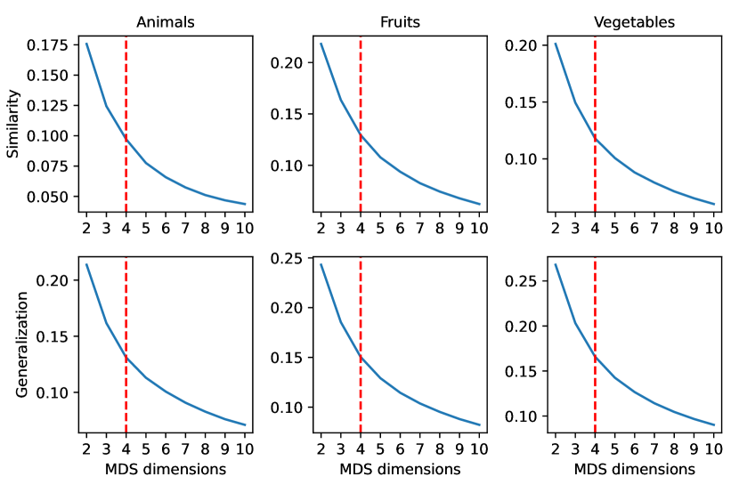
Figure 5: Non-metric MDS stress curves for the various domains considered in the present work as a function of MDS dimensions. Based on this analysis we selected the first dimensionality ($d=4$, marked in dashed red vertical lines) for which all stress values across all datasets dropped below $0.2$ (a standard threshold above which MDS fit is deemed poor [13]).

Multidimensional scaling. Given a dissimilarity matrix $\Delta_{ij}$, MDS embeddings $z$ were obtained using the manifold.MDS method from the scikit-learn Python library [18] with a maximum iteration limit of 10,000 and a convergence tolerance of 1e-100. Embeddings were computed in two steps: first metric MDS was applied to get an initial embedding which was then used to initialize non-metric MDS. We chose a $d=4$ dimensionality for the embedding space based on an MDS stress curve analysis (shown in Supplementary Figure 5; for visualization purposes only we used $d=2$ in the figures below) whereby the first dimension $d$ for which all stress values across all datasets dropped below $0.2$ was selected (a standard threshold above which MDS fit is deemed poor; [13]). Finally, to construct generalization gradients we computed Euclidean distance between all MDS embedding vectors $d_{ij}=||z_{i}-z_{j}||_{2}$ and combined them with their corresponding similarity scores $s_{ij}$ to produce the two-dimensional set $\mathcal{D}=\{(d_{ij},s_{ij})\}$. We analyzed the resulting generalization gradients in two complementary ways, namely, by directly fitting curve models to the raw set $\mathcal{D}$, and by fitting them to a binned version of $\mathcal{D}$. The former served as a conservative test, and the latter as more balanced one meant to evaluate the average curve and to take into account the fact that different regions of the generalization gradient have different densities (e.g., high similarity pairs are much less common than low similarity pairs which can over-emphasize the tail of the gradient). The binning was done by dividing the distances $\{d_{ij}\}$ into 100 bins and then computing the average $d_{ij}$ and $s_{ij}$ within each bin and their standard errors.

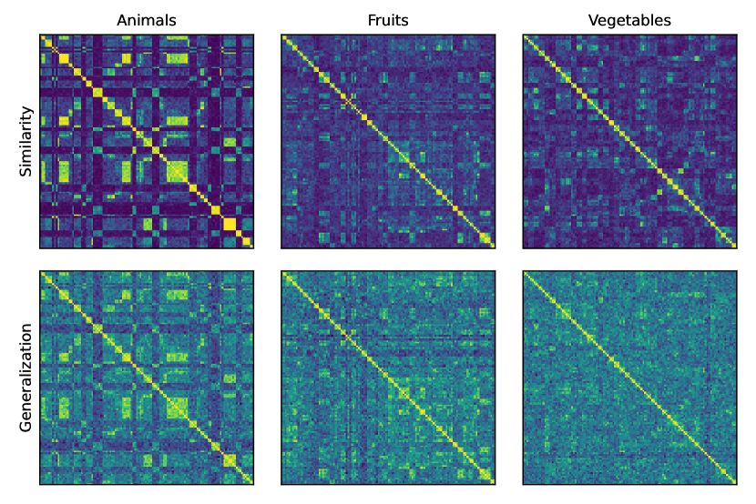
Figure 2: Similarity matrices over the different domains of natural images and the two judgment elicitation tasks considered, namely, direct similarity judgments (top) and generalization judgments (bottom).

Model fitting and evaluation. To test the universal law, we evaluated the extent to which an exponential function of the form $g(x)=ae^{-bx}+c$ could account for the generalization gradients $\mathcal{D}$ relative to three other models of increasing complexity, namely, a simple linear model $g(x)=ax+b$, a quadratic model $g(x)=ax^{2}+bx+c$ (same complexity as exponential but with the option of being either concave or convex), and a flexible generalized additive model (GAM), i.e., a model of the form $g(x)=\alpha+\sum_{i}\beta_{i}f_{i}(x)$ where $f_{i}(x)$ is a basis of cubic splines [9], as well as the intrinsic inter-rater variability of the data. To fit the exponential, linear, and quadratic models we used the curve_fit least squares optimizer in scipy, and to fit the GAM we used the LinearGAM method of the pygam package [26] which by default uses 20 basis functions and optimizes the model parameters in a grid-search manner. For model evaluation, and to accommodate both for the possibility of over-fitting and to adjust for degrees of freedom, we performed a split-half bootstrap analysis whereby 100 data splits were produced by randomly dividing the ratings per image pair in half and then producing two generalization gradients $\mathcal{D}_{h_{1}}$ and $\mathcal{D}_{h_{2}}$ to which the model was fitted yielding two sets of predictions $\{s^{\prime}_{ij}\}_{h_{1}}$ and $\{s^{\prime}_{ij}\}_{h_{2}}$. We then computed the following Pearson correlation coefficients between the data-model sets $\{s_{ij}\}_{h_{1}}$, $\{s^{\prime}_{ij}\}_{h_{1}}$ and $\{s_{ij}\}_{h_{2}}$, $\{s^{\prime}_{ij}\}_{h_{2}}$: $r_{dd}$ data-data correlation, $r_{mm}$ model-model correlation, $r_{dm}$ data-model correlation (there are two splits for each randomized split half, and thus there are two ways to compute this which we averaged), and $r_{c}=r_{dm}/\sqrt{r_{dd}r_{mm}}$ the data-model correlation corrected for attenuation. In addition, we provide the coefficient of determination (variance explained) $R^{2}$ for each of the fitted models, as well as, the Bayesian Information Criterion (BIC) for model selection which trades-off model complexity with goodness of fit [23]. We used the Gaussian BIC formula which is given by $\text{BIC}=n\log(\text{RSS}/n)+k\log n$ where $\text{RSS}=\sum_{i}(x_{i}-\hat{x}_{i})^{2}$ is the residual sum of squares between data and model, $n$ is the number of data points and $k$ is the number of fitted parameters. Finally, since only the relative BIC score is meaningful and because we are specifically interested in how models perform relative to the exponential solution, we report BIC scores relative to that solution $\Delta\text{BIC}=\text{BIC}_{\text{model}}-\text{BIC}_{\text{exponential}}$. We note that in computing all metrics we excluded trivial self-similarity points $(d=0,s=1)$ to prevent artificial inflation of values.

3 Results

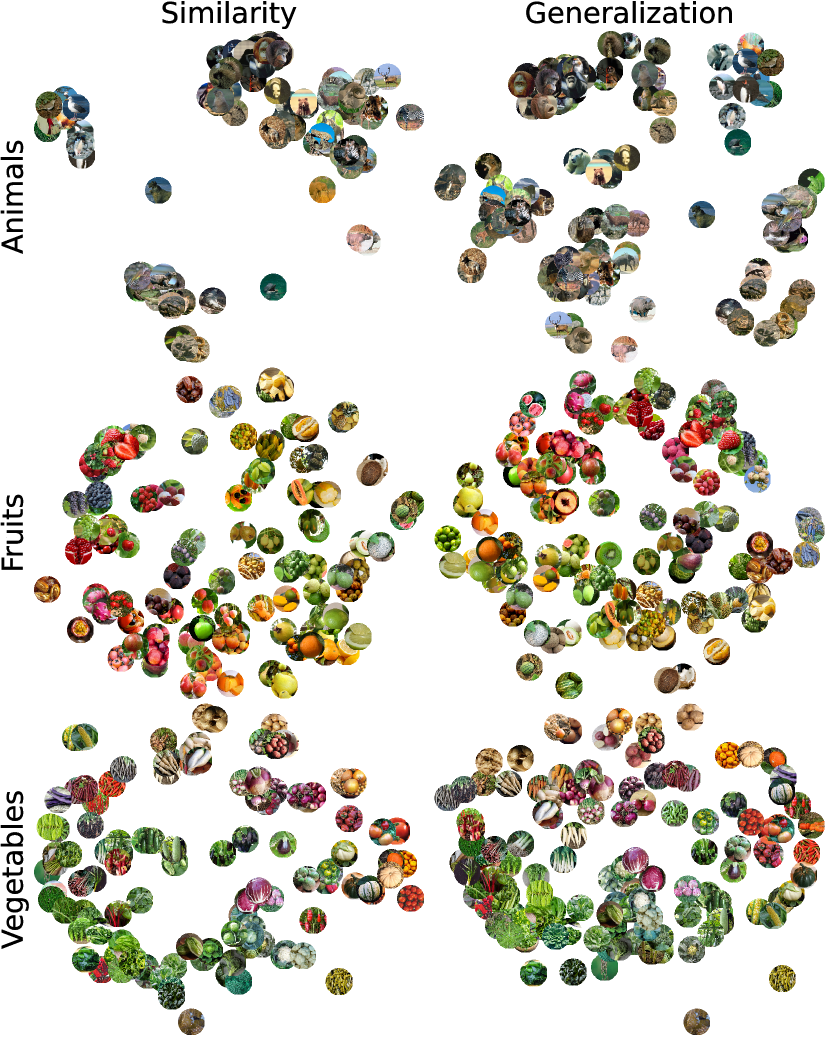
Figure 3: Two-dimensional MDS embeddings for the similarity and generalization data with the raw image stimuli from the different natural categories overlaid.

The average similarity matrices over the different domains and tasks are summarized in Figure 2. The first thing to observe is that the generalization and similarity judgment tasks yield results that are significantly correlated across domains, with a Pearson correlation of $r=.71$ (95% CI $[.69,.74]$) for animals, $r=.55$ (95% CI $[.52,.58]$) for fruits, and $r=.36$ (95% CI $[.33,.40]$) for vegetables (CIs bootstrapped over participants with 100 repetitions). This is consistent with the expectation that generalization over blank properties and similarity judgments capture shared variance [12].

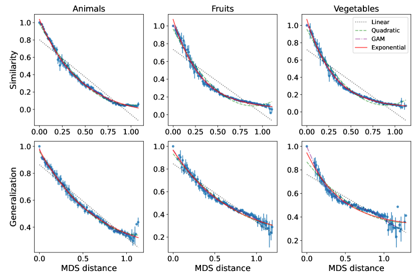
Figure 4: Generalization gradients across domains of natural images and tasks with the optimal model fits overlaid. Error bars indicate 95% confidence intervals.

Next, to get a better sense of the psychological content of those spaces, we visualized their two-dimensional MDS solutions in Figure 3. All three domains revealed a semantically structured organization of the stimuli. In the case of animal images, distinct and interpretable organization schemes emerged, corresponding to animal categories such as herbivores, carnivores, amphibians, reptiles, and birds. In the case of fruits and vegetables the distribution is more continuous, with color serving as a clear semantic axis, with interpretable subclasses occupying different areas of the space such as citrus fruits and berries in the case of fruits, and whether the vegetable grows above or below the ground in the case of vegetables. These results are consistent with the findings of [20] in the case of similarity and extend them to generalization, implying again that both tasks are capturing shared semantic content.

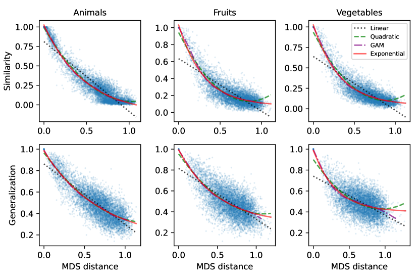
Figure 6: Raw generalization gradients across domains of natural images and tasks with the optimal fitted models overlaid.

We are now ready to analyze the generalization gradients for each of the conditions and test to what extent they can be explained by the different models. The average binned gradients along with their optimal fit for all models are shown in Figure 4 (see Methods; raw gradients are shown in Supplementary Figure 6; explicit fitted parameter values and their CIs are provided in Supplementary Tables 3-5 and 8-10 for the raw and binned analyses, respectively). As can be seen, the scatter points appear to follow a concave trend, with the similarity data in particular tightly tracking the exponential curve, which also overlaps substantially with the quadratic and GAM models. The linear model, on the other hand, appears to find some intermediate compromise due to its limited flexibility. To quantify this, we provide the full list of evaluation metrics on the raw gradients in Tables 1-2 (see Supplementary Tables 6-7 for additional metrics; see also Tables 11-12 and 13-14 for the binned equivalent). The exponential function provides an excellent model for the data with an average model-data Pearson correlation of $r_{c}=.96$ (corrected for attenuation, see Methods). To see where the exponential model stands with respect to the different models in each condition, we bootstrapped the difference in variance explained $\Delta R^{2}=R^{2}_{\text{exponential}}-R^{2}_{\text{model}}$, and the Bayesian Information Criterion $\Delta\text{BIC}$ (see Methods) between the exponential model and the other models.
Starting from the domain of similarity, we found that the exponential model outperformed the linear model in all three domains, with $\Delta R^{2}$ 95% CIs given by $[.04,.10]$, $[.13,.14]$, $[.13,.14]$ for animals, fruits, and vegetables, respectively. The same pattern holds for the corresponding $\Delta\text{BIC}$ CIs (i.e., when penalizing for complexity), $[2644,2921]$, $[1830,2110]$, $[2185,2458]$ (positive values favor exponential in our definition of $\Delta\text{BIC}$). As for the quadratic solution, the models performed practically the same (with a slight boost for the exponential) with $\Delta R^{2}$ CIs given by $[-.001,.001]$, $[.009,.017]$, and $[.010,.014]$ for animals, fruits and vegetables, respectively (and likewise for the corresponding $\Delta\text{BIC}$, $[-40,31]$, $[151,265]$, and $[193,280]$). Crucially, however, all quadratic solutions converged on concave curvature with strictly positive second derivatives $g^{\prime\prime}(x)=2a>0$ with CIs $[1.77,1.85]$, $[2.36,2.24]$, and $[2.22,2.31]$ (see Table 5) consistent with the universal law hypothesis. Finally, for the flexible GAM model, we found that it was unable to meaningfully improve on the exponential model despite its flexibility, with $\Delta R^{2}$ CIs given by $[-.006,-.002]$, $[-.008,-.004]$, $[-.006,-.002]$, and $\Delta\text{BIC}$ CIs given by $[-123,84]$, $[19,98]$, $[30,110]$, for animals, fruits and vegetables, respectively.
As for the generalization data, we observed a similar pattern, namely, the exponential model outpeformed the linear ($\Delta R^{2}$ CIs, $[.019,.025]$, $[.014,.024]$, $[.012,.024]$, and $\Delta\text{BIC}$ CIs, $[276,366]$, $[135,242]$, $[103,214]$, for animals, fruits and vegetables, respectively). Likewise, the quadratic model performed on par with the exponential model ($\Delta R^{2}$ CIs, $[.001,.001]$, $[.002,.004]$, $[.008,.012]$, and $\Delta\text{BIC}$ CIs, $[4,17]$, $[28,45]$, $[68,109]$), and was strictly concave on all domains ($g^{\prime\prime}(x)=2a>0$ with CIs $[0.82,0.93]$, $[0.90,1.05]$, and $[0.99,1.13]$). Finally, the GAM model did not improve on the exponential model despite the additional degrees of freedom $\Delta R^{2}$ CIs, $[.002,.000]$, $[-.004,.000]$, $[-.009,.003]$, and $\Delta\text{BIC}$ CIs, $[133,163]$, $[120,151]$, $[75,128]$). Viewed together, these results provide direct evidence for the universal law of generalization.

Table 1: Full list of model evaluation metrics on the similarity tasks and their 95% confidence intervals based on split-half bootstrap over trials with 100 repetitions.

Category	Model	$R^{2}$	$\delta R^{2}$	$r_{md}$	$\delta r_{md}$	$r_{c}$	$\delta r_{c}$	$\Delta\text{BIC}$	$\delta\Delta\text{BIC}$
Animals	Exponential	0.854	0.005	0.906	0.002	0.982	0.01	0.0	0.0
Animals	Linear	0.784	0.006	0.868	0.003	0.968	0.033	2782.613	138.579
Animals	Quadratic	0.854	0.005	0.906	0.002	0.98	0.008	-4.387	35.575
Animals	GAM	0.858	0.005	0.907	0.003	0.983	0.008	-19.403	103.188
Fruits	Exponential	0.575	0.014	0.69	0.009	0.998	0.022	0.0	0.0
Fruits	Linear	0.441	0.014	0.615	0.008	0.933	0.048	1970.43	139.787
Fruits	Quadratic	0.563	0.015	0.683	0.009	0.991	0.021	207.94	56.923
Fruits	GAM	0.581	0.014	0.692	0.009	0.997	0.019	58.402	39.297
Vegetables	Exponential	0.645	0.01	0.75	0.007	0.99	0.009	0.0	0.0
Vegetables	Linear	0.509	0.01	0.679	0.005	0.902	0.015	2321.842	136.625
Vegetables	Quadratic	0.633	0.011	0.743	0.007	0.983	0.009	236.349	43.698
Vegetables	GAM	0.649	0.01	0.752	0.007	0.992	0.008	69.554	39.957

• Note: The measures are: $R^{2}$ coefficient of determination, $r_{md}$ model-data Pearson correlation, $r_{c}$ model-data correlation corrected for attenuation, and $\Delta\text{BIC}$ the Bayesian Information Criterion (BIC) relative to the exponential model in each category. $\delta$ indicates 95% confidence error (i.e., $\delta X=1.96\cdot\sigma_{X}$ where $\sigma_{X}$ is the standard deviation of $X$). See Methods for full details.

Table 2: Full list of model evaluation metrics on the generalization tasks and their 95% confidence intervals based on split-half bootstrap over trials with 100 repetitions.

Category	Model	$R^{2}$	$\delta R^{2}$	$r_{md}$	$\delta r_{md}$	$r_{c}$	$\delta r_{c}$	$\Delta\text{BIC}$	$\delta\Delta\text{BIC}$
Animals	Exponential	0.522	0.031	0.655	0.01	0.951	0.015	0.0	0.0
Animals	Linear	0.5	0.032	0.641	0.01	0.946	0.026	320.879	44.845
Animals	Quadratic	0.521	0.031	0.656	0.01	0.95	0.014	10.57	6.792
Animals	GAM	0.523	0.031	0.656	0.01	0.951	0.015	148.101	14.716
Fruits	Exponential	0.32	0.023	0.459	0.012	0.875	0.023	0.0	0.0
Fruits	Linear	0.301	0.022	0.449	0.012	0.863	0.028	188.706	53.238
Fruits	Quadratic	0.316	0.023	0.458	0.012	0.872	0.023	36.861	8.414
Fruits	GAM	0.322	0.023	0.46	0.012	0.879	0.024	135.5	15.998
Vegetables	Exponential	0.202	0.016	0.265	0.016	0.928	0.047	0.0	0.0
Vegetables	Linear	0.184	0.014	0.263	0.016	0.903	0.048	158.541	55.12
Vegetables	Quadratic	0.192	0.015	0.261	0.016	0.918	0.048	88.4	20.665
Vegetables	GAM	0.209	0.016	0.27	0.016	0.933	0.045	101.458	26.378

• Note: See Table 1 for definitions of the various evaluation metrics.

4 Discussion

Shepard’s universal law of generalization stands out as a theoretical claim about cognition in its intended scope, covering all intelligent entities and all stimuli. However, previous work had only evaluated it using relatively small, simple sets of stimuli. We assessed its performance in large sets of high-dimensional natural images comprising more than 600,000 human judgments. Our results provide robust evidence for the validity of the universal law and extend its long research tradition into rich naturalistic domains. By analyzing both similarity and generalization judgments, we also confirmed that generalization over blank properties and default similarity judgments indeed capture shared sources of variance even when the dimensionality of the space is particularly large.

There are a number of limitations of the present work that can be further addressed by future research. First, our population was limited to online US participants to allow for efficient scaling of data crowdsourcing. However, cross-cultural research is necessary in order to evaluate the extent to which our findings generalize beyond US populations and English speakers [3]. Nevertheless, the fact that we focused specifically on widespread natural categories should facilitate such an investigation. Second, in the present work we restricted ourselves to the visual modality, but one could equally consider natural categories in other primary modalities like the auditory and audio-visual (e.g., environmental sounds and scenes). While perhaps not as common as images, large behavioral datasets over such domains are becoming increasingly more accessible due to the growing interest in multi-modal models in the machine learning community (see e.g., [6]; [15]). Third, future work could explore how the results of our generalization analysis vary when other blank properties are considered. Indeed, one might expect that different blank properties may activate different forms of inductive reasoning [12] as well as inter-subject variation. The extent to which these too support the universal law of generalization is an open question that requires further investigation. Finally, naturalistic stimuli provide much more space than artificial stimuli for interrogating the relationship between generalization and similarity. Our results showed a significant correlation between similarity and generalization, but it varied significantly across domains. This raises questions such as what features of a complex stimulus people rely on when generalizing from one stimulus to another, and how their weights differ when people evaluate similarity. We hope to engage with these questions in future work.

More broadly, our work showcases the prospects of scaling up psychological research, providing unprecedented precision for tests of foundational hypotheses in cognitive science, as well as new avenues for exploration of naturalistic stimuli. If our goal is to identify universal psychological principles underlying human cognition, being able to test those principles in naturalistic settings is essential to making strong claims about their universality. Finding that the universal law of generalization holds for natural images provides support for its use as a component of other cognitive models applied to these rich and complex stimuli (e.g., [2]; [25]), laying the groundwork for more extensive deployment and testing of models of human behavior based on psychological theory.

Competing Interests. The authors declare no competing interests.

Acknowledgments. This work was supported by grant 61454 from the John Templeton Foundation.

Appendix A Supplementary Information

Table 3: Exponential model parameters of the form $g(x)=ae^{-bx}+c$. Errors ($\delta$) indicate 95% confidence intervals bootstrapped over trials with 100 repetitions.

Task	Category	$a$	$\delta a$	$b$	$\delta b$	$c$	$\delta c$
Similarity	Animals	1.179	0.009	2.022	0.043	-0.138	0.009
Similarity	Fruits	0.969	0.008	3.243	0.075	0.072	0.005
Similarity	Vegetables	1.005	0.007	3.08	0.056	0.032	0.005
Generalization	Animals	0.844	0.018	1.525	0.085	0.154	0.022
Generalization	Fruits	0.711	0.012	2.029	0.114	0.28	0.016
Generalization	Vegetables	0.604	0.009	2.916	0.144	0.378	0.01

Table 4: Linear model parameters of the form $g(x)=ax+b$. Errors ($\delta$) indicate 95% confidence intervals bootstrapped over trials with 100 repetitions.

Task	Category	$a$	$\delta a$	$b$	$\delta b$
Similarity	Animals	-0.917	0.005	0.827	0.003
Similarity	Fruits	-0.629	0.008	0.639	0.006
Similarity	Vegetables	-0.671	0.007	0.646	0.005
Generalization	Animals	-0.568	0.007	0.86	0.005
Generalization	Fruits	-0.484	0.008	0.807	0.006
Generalization	Vegetables	-0.39	0.009	0.745	0.006

Table 5: Quadratic model parameters of the form $g(x)=ax^{2}+bx+c$. Errors ($\delta$) indicate 95% confidence intervals bootstrapped over trials with 100 repetitions.

Task	Category	$a$	$\delta a$	$b$	$\delta b$	$c$	$\delta c$
Similarity	Animals	0.906	0.021	-1.872	0.023	1.007	0.005
Similarity	Fruits	1.152	0.03	-1.951	0.033	0.957	0.009
Similarity	Vegetables	1.134	0.024	-1.968	0.026	0.956	0.007
Generalization	Animals	0.436	0.027	-1.069	0.03	0.977	0.007
Generalization	Fruits	0.488	0.036	-1.058	0.04	0.951	0.01
Generalization	Vegetables	0.528	0.035	-1.017	0.039	0.906	0.01

Table 6: Complementary list of evaluation measures on the similarity tasks and their 95% confidence intervals based on split-half bootstrap over trials with 100 repetitions.

Category	Model	$r_{dd}$	$\delta r_{dd}$	$r_{mm}$	$\delta r_{mm}$	$r_{md}$	$\delta r_{md}$
Animals	Exponential	0.89	0.004	0.956	0.019	0.906	0.002
Animals	Linear	0.89	0.004	0.905	0.063	0.868	0.003
Animals	Quadratic	0.89	0.004	0.96	0.016	0.906	0.002
Animals	GAM	0.89	0.004	0.958	0.016	0.907	0.003
Fruits	Exponential	0.591	0.011	0.808	0.041	0.69	0.009
Fruits	Linear	0.591	0.011	0.737	0.083	0.615	0.008
Fruits	Quadratic	0.591	0.011	0.803	0.039	0.683	0.009
Fruits	GAM	0.591	0.011	0.815	0.036	0.692	0.009
Vegetables	Exponential	0.64	0.01	0.897	0.018	0.75	0.007
Vegetables	Linear	0.64	0.01	0.884	0.033	0.679	0.005
Vegetables	Quadratic	0.64	0.01	0.893	0.019	0.743	0.007
Vegetables	GAM	0.64	0.01	0.898	0.017	0.752	0.007

• Note: The measures are: $r_{dd}$ data-data Pearson correlation, $r_{mm}$ model-model Pearson correlation, and $r_{md}$ model-data Pearson correlation. $\delta$ indicates 95% confidence error (i.e., $\delta X=1.96\cdot\sigma_{X}$ where $\sigma_{X}$ is the standard deviation of $X$).

Table 7: Complementary list of evaluation measures on the generalization tasks and their 95% confidence intervals based on split-half bootstrap over trials with 100 repetitions.

Category	Model	$r_{dd}$	$\delta r_{dd}$	$r_{mm}$	$\delta r_{mm}$	$r_{md}$	$\delta r_{md}$
Animals	Exponential	0.577	0.011	0.823	0.037	0.655	0.01
Animals	Linear	0.577	0.011	0.796	0.056	0.641	0.01
Animals	Quadratic	0.577	0.011	0.825	0.036	0.656	0.01
Animals	GAM	0.577	0.011	0.824	0.037	0.656	0.01
Fruits	Exponential	0.417	0.013	0.661	0.041	0.459	0.012
Fruits	Linear	0.417	0.013	0.649	0.049	0.449	0.012
Fruits	Quadratic	0.417	0.013	0.66	0.04	0.458	0.012
Fruits	GAM	0.417	0.013	0.658	0.042	0.46	0.012
Vegetables	Exponential	0.188	0.016	0.437	0.053	0.265	0.016
Vegetables	Linear	0.188	0.016	0.454	0.061	0.263	0.016
Vegetables	Quadratic	0.188	0.016	0.432	0.055	0.261	0.016
Vegetables	GAM	0.188	0.016	0.447	0.054	0.27	0.016

• Note: See Table 6 for definition of the various metrics.

Appendix B Binned Analysis

Table 8: Exponential model parameters of the form $g(x)=ae^{-bx}+c$. Errors ($\delta$) indicate 95% confidence intervals bootstrapped over trials with 100 repetitions and $n=100$ bins.

Task	Category	$a$	$\delta a$	$b$	$\delta b$	$c$	$\delta c$
Similarity	Animals	1.154	0.017	2.194	0.101	-0.097	0.021
Similarity	Fruits	1.059	0.028	3.396	0.14	0.071	0.01
Similarity	Vegetables	1.069	0.022	3.195	0.129	0.032	0.009
Generalization	Animals	0.844	0.044	1.525	0.201	0.153	0.056
Generalization	Fruits	0.75	0.044	1.769	0.347	0.229	0.068
Generalization	Vegetables	0.608	0.036	2.546	0.661	0.344	0.063

Table 9: Linear model parameters of the form $g(x)=ax+b$. Errors ($\delta$) indicate 95% confidence intervals bootstrapped over trials with 100 repetitions and $n=100$ bins.

Task	Category	$a$	$\delta a$	$b$	$\delta b$
Similarity	Animals	-0.882	0.046	0.817	0.018
Similarity	Fruits	-0.723	0.03	0.721	0.016
Similarity	Vegetables	-0.77	0.032	0.731	0.015
Generalization	Animals	-0.57	0.02	0.869	0.01
Generalization	Fruits	-0.491	0.02	0.819	0.012
Generalization	Vegetables	-0.385	0.03	0.747	0.016

Table 10: Quadratic model parameters of the form $g(x)=ax^{2}+bx+c$. Errors ($\delta$) indicate 95% confidence intervals bootstrapped over trials with 100 repetitions and $n=100$ bins.

Task	Category	$a$	$\delta a$	$b$	$\delta b$	$c$	$\delta c$
Similarity	Animals	0.958	0.033	-1.919	0.033	1.008	0.008
Similarity	Fruits	1.203	0.086	-2.057	0.093	0.992	0.024
Similarity	Vegetables	1.189	0.077	-2.067	0.081	0.984	0.019
Generalization	Animals	0.43	0.072	-1.063	0.073	0.974	0.015
Generalization	Fruits	0.386	0.099	-0.96	0.11	0.93	0.026
Generalization	Vegetables	0.37	0.172	-0.841	0.189	0.858	0.043

Table 11: Full list of model evaluation metrics on the similarity tasks and their 95% confidence intervals based on split-half bootstrap over trials with 100 repetitions and $n=100$ bins.

Category	Model	$R^{2}$	$\delta R^{2}$	$r_{md}$	$\delta r_{md}$	$r_{c}$	$\delta r_{c}$	$\Delta\text{BIC}$	$\delta\Delta\text{BIC}$
Animals	Exponential	0.994	0.002	0.997	0.001	0.999	0.001	0.0	0.0
Animals	Linear	0.911	0.014	0.954	0.005	0.956	0.005	257.735	27.564
Animals	Quadratic	0.993	0.002	0.996	0.001	0.998	0.001	16.567	20.269
Animals	GAM	0.997	0.001	0.998	0.001	1.0	0.0	21.103	40.222
Fruits	Exponential	0.986	0.005	0.993	0.002	0.998	0.002	0.0	0.0
Fruits	Linear	0.812	0.018	0.902	0.005	0.906	0.006	226.335	31.753
Fruits	Quadratic	0.969	0.008	0.984	0.003	0.989	0.003	71.777	25.337
Fruits	GAM	0.991	0.005	0.994	0.002	1.0	0.001	39.543	30.356
Vegetables	Exponential	0.991	0.004	0.995	0.001	0.999	0.001	0.0	0.0
Vegetables	Linear	0.837	0.014	0.915	0.004	0.919	0.004	251.392	35.803
Vegetables	Quadratic	0.979	0.005	0.989	0.002	0.993	0.002	72.835	31.745
Vegetables	GAM	0.993	0.004	0.996	0.002	1.0	0.001	52.324	28.149

• Note: The measures are: $R^{2}$ coefficient of determination, $r_{md}$ model-data Pearson correlation, $r_{c}$ model-data correlation corrected for attenuation, and $\Delta\text{BIC}$ the Bayesian Information Criterion (BIC) relative to the exponential model in each category. $\delta$ indicates 95% confidence error (i.e., $\delta X=1.96\cdot\sigma_{X}$ where $\sigma_{X}$ is the standard deviation of $X$). See Methods for full details.

Table 12: Full list of model evaluation metrics on the generalization tasks and their 95% confidence intervals based on split-half bootstrap over trials with 100 repetitions and $n=100$ bins.

Category	Model	$R^{2}$	$\delta R^{2}$	$r_{md}$	$\delta r_{md}$	$r_{c}$	$\delta r_{c}$	$\Delta\text{BIC}$	$\delta\Delta\text{BIC}$
Animals	Exponential	0.989	0.01	0.994	0.004	1.0	0.003	0.0	0.0
Animals	Linear	0.951	0.02	0.975	0.007	0.98	0.007	125.869	39.802
Animals	Quadratic	0.989	0.008	0.994	0.003	0.999	0.003	3.683	16.468
Animals	GAM	0.992	0.004	0.993	0.006	1.0	0.001	53.514	53.277
Fruits	Exponential	0.97	0.016	0.985	0.006	0.997	0.006	0.0	0.0
Fruits	Linear	0.932	0.02	0.966	0.006	0.978	0.007	66.156	44.537
Fruits	Quadratic	0.965	0.017	0.982	0.007	0.994	0.006	13.808	9.359
Fruits	GAM	0.982	0.01	0.986	0.009	1.0	0.003	40.117	46.13
Vegetables	Exponential	0.935	0.052	0.965	0.021	0.991	0.017	0.0	0.0
Vegetables	Linear	0.888	0.051	0.945	0.018	0.97	0.02	39.1	54.258
Vegetables	Quadratic	0.924	0.044	0.958	0.023	0.985	0.016	12.989	18.99
Vegetables	GAM	0.974	0.015	0.964	0.039	1.0	0.005	9.844	63.035

• Note: See Table 1 for definitions of the various evaluation metrics.

Table 13: Complementary list of evaluation measures on the similarity tasks and their 95% confidence intervals based on split-half bootstrap over trials with 100 repetitions and $n=100$ bins.

Category	Model	$r_{dd}$	$\delta r_{dd}$	$r_{mm}$	$\delta r_{mm}$	$r_{md}$	$\delta r_{md}$
Animals	Exponential	0.996	0.002	1.0	0.0	0.997	0.001
Animals	Linear	0.996	0.002	1.0	0.0	0.954	0.005
Animals	Quadratic	0.996	0.002	1.0	0.0	0.996	0.001
Animals	GAM	0.996	0.002	0.999	0.001	0.998	0.001
Fruits	Exponential	0.99	0.005	1.0	0.0	0.993	0.002
Fruits	Linear	0.99	0.005	1.0	0.0	0.902	0.005
Fruits	Quadratic	0.99	0.005	1.0	0.0	0.984	0.003
Fruits	GAM	0.99	0.005	0.999	0.001	0.994	0.002
Vegetables	Exponential	0.992	0.004	1.0	0.0	0.995	0.001
Vegetables	Linear	0.992	0.004	1.0	0.0	0.915	0.004
Vegetables	Quadratic	0.992	0.004	1.0	0.0	0.989	0.002
Vegetables	GAM	0.992	0.004	0.999	0.001	0.996	0.002

• Note: The measures are: $r_{dd}$ data-data Pearson correlation, $r_{mm}$ model-model Pearson correlation, and $r_{md}$ model-data Pearson correlation. $\delta$ indicates 95% confidence error (i.e., $\delta X=1.96\cdot\sigma_{X}$ where $\sigma_{X}$ is the standard deviation of $X$).

Table 14: Complementary list of evaluation measures on the generalization tasks and their 95% confidence intervals based on split-half bootstrap over trials with 100 repetitions and $n=100$ bins.

Category	Model	$r_{dd}$	$\delta r_{dd}$	$r_{mm}$	$\delta r_{mm}$	$r_{md}$	$\delta r_{md}$
Animals	Exponential	0.989	0.007	1.0	0.001	0.994	0.004
Animals	Linear	0.989	0.007	1.0	0.0	0.975	0.007
Animals	Quadratic	0.989	0.007	1.0	0.001	0.994	0.003
Animals	GAM	0.989	0.007	0.998	0.006	0.993	0.006
Fruits	Exponential	0.976	0.014	1.0	0.001	0.985	0.006
Fruits	Linear	0.976	0.014	1.0	0.0	0.966	0.006
Fruits	Quadratic	0.976	0.014	0.999	0.002	0.982	0.007
Fruits	GAM	0.976	0.014	0.996	0.008	0.986	0.009
Vegetables	Exponential	0.95	0.042	0.998	0.004	0.965	0.021
Vegetables	Linear	0.95	0.042	1.0	0.0	0.945	0.018
Vegetables	Quadratic	0.95	0.042	0.995	0.011	0.958	0.023
Vegetables	GAM	0.95	0.042	0.979	0.037	0.964	0.039

• Note: See Table 13 for definition of the various metrics.

References

- [1] Edmond Awad et al. “The moral machine experiment” In Nature 563.7729 Nature Publishing Group, 2018, pp. 59–64
- [2] Ruairidh M Battleday, Joshua C Peterson and Thomas L Griffiths “Capturing human categorization of natural images by combining deep networks and cognitive models” In Nature Communications 11.1 Nature Publishing Group, 2020, pp. 1–14
- [3] Damián E. Blasi et al. “Over-reliance on English hinders cognitive science” In Trends in Cognitive Sciences 26.12, 2022, pp. 1153–1170
- [4] Nick Chater and Paul MB Vitányi “The generalized universal law of generalization” In Journal of Mathematical Psychology 47.3 Elsevier, 2003, pp. 346–369
- [5] Ken Cheng “Shepard’s universal law supported by honeybees in spatial generalization” In Psychological Science 11.5 SAGE Publications Sage CA: Los Angeles, CA, 2000, pp. 403–408
- [6] Jort F Gemmeke et al. “Audio set: An ontology and human-labeled dataset for audio events” In 2017 IEEE international conference on acoustics, speech and signal processing (ICASSP), 2017, pp. 776–780 IEEE
- [7] Stefano Ghirlanda and Magnus Enquist “A century of generalization” In Animal Behaviour 66.1, 2003, pp. 15–36
- [8] Peter Harrison et al. “Gibbs Sampling with People” In Advances in Neural Information Processing Systems 33 Curran Associates, Inc., 2020, pp. 10659–10671
- [9] Trevor Hastie, Robert Tibshirani, Jerome H Friedman and Jerome H Friedman “The elements of statistical learning: data mining, inference, and prediction” Springer, 2009
- [10] Martin N Hebart, Charles Y Zheng, Francisco Pereira and Chris I Baker “Revealing the multidimensional mental representations of natural objects underlying human similarity judgements” In Nature Human Behaviour 4.11 Nature Publishing Group UK London, 2020, pp. 1173–1185
- [11] Aditi Jha, Joshua C Peterson and Thomas L Griffiths “Extracting low-dimensional psychological representations from convolutional neural networks” In Cognitive Science 47.1 Wiley Online Library, 2023, pp. e13226
- [12] Charles Kemp and Joshua B Tenenbaum “Structured statistical models of inductive reasoning.” In Psychological Review 116.1 American Psychological Association, 2009, pp. 20
- [13] Joseph B Kruskal “Multidimensional scaling by optimizing goodness of fit to a nonmetric hypothesis” In Psychometrika 29.1 Springer, 1964, pp. 1–27
- [14] Raja Marjieh et al. “Reshaping musical consonance with timbral manipulations and massive online experiments” In bioRxiv Cold Spring Harbor Laboratory, 2022, pp. 2022–06
- [15] Raja Marjieh et al. “Words are all you need? Language as an approximation for human similarity judgments” In The Eleventh International Conference on Learning Representations, 2023
- [16] In Jae Myung and Roger N Shepard “Maximum entropy inference and stimulus generalization” In Journal of Mathematical Psychology 40.4, 1996, pp. 342–347
- [17] Daniel N Osherson et al. “Category-based induction.” In Psychological Review 97.2 American Psychological Association, 1990, pp. 185
- [18] F. Pedregosa et al. “Scikit-learn: Machine Learning in Python” In Journal of Machine Learning Research 12, 2011, pp. 2825–2830
- [19] Michael Peer, Iva K Brunec, Nora S Newcombe and Russell A Epstein “Structuring knowledge with cognitive maps and cognitive graphs” In Trends in cognitive sciences 25.1 Elsevier, 2021, pp. 37–54
- [20] Joshua C. Peterson, Joshua T. Abbott and Thomas L. Griffiths “Evaluating (and Improving) the Correspondence Between Deep Neural Networks and Human Representations” In Cognitive Science 42.8, 2018, pp. 2648–2669
- [21] Joshua C Peterson et al. “Using large-scale experiments and machine learning to discover theories of human decision-making” In Science 372.6547 American Association for the Advancement of Science, 2021, pp. 1209–1214
- [22] Joshua C Peterson and Thomas L Griffiths “Evidence for the size principle in semantic and perceptual domains” In arXiv preprint arXiv:1705.03260, 2017
- [23] Maurice Bertram Priestley “Spectral analysis and time series: probability and mathematical statistics” Academic Press, 1981
- [24] Brett D Roads and Bradley C Love “Enriching imagenet with human similarity judgments and psychological embeddings” In Proceedings of the IEEE/CVF Conference on Computer Vision and Pattern Recognition, 2021, pp. 3547–3557
- [25] Craig A Sanders and Robert M Nosofsky “Training deep networks to construct a psychological feature space for a natural-object category domain” In Computational Brain & Behavior 3, 2020, pp. 229–251
- [26] Daniel Servén and Charlie Brummitt “pygam: Generalized additive models in python” In Zenodo. doi 10, 2018
- [27] Roger N Shepard “The analysis of proximities: multidimensional scaling with an unknown distance function. I.” In Psychometrika 27.2, 1962, pp. 125–140
- [28] Roger N. Shepard “Multidimensional scaling, tree-fitting, and clustering” In Science 210.4468 American Association for the Advancement of Science, 1980, pp. 390–398
- [29] Roger N Shepard “Toward a universal law of generalization for psychological science” In Science 237.4820 American Association for the Advancement of Science, 1987, pp. 1317–1323
- [30] Chris R. Sims “Efficient coding explains the universal law of generalization in human perception” In Science 360.6389, 2018, pp. 652–656
- [31] Mark Steyvers “Multidimensional scaling” In Encyclopedia of cognitive science 1, 2002
- [32] Joshua B. Tenenbaum and Thomas L. Griffiths “Generalization, similarity, and Bayesian inference” In Behavioral and Brain Sciences 24.4 Cambridge University Press, 2001, pp. 629–640
- [33] Amos Tversky “Features of similarity.” In Psychological Review 84.4, 1977, pp. 327
- [34] Amos Tversky and J Hutchinson “Nearest neighbor analysis of psychological spaces.” In Psychological review 93.1 American Psychological Association, 1986, pp. 3