Bayesian inversion for Electrical Impedance Tomography by sparse interpolation

Abstract.

We study the Electrical Impedance Tomography Bayesian inverse problem for recovering the conductivity given noisy measurements of the voltage on some boundary surface electrodes. The uncertain conductivity depends linearly on a countable number of uniformly distributed random parameters in a compact interval, with the coefficient functions in the linear expansion decaying with an algebraic rate. We analyze the surrogate Markov Chain Monte Carlo (MCMC) approach for sampling the posterior probability measure, where the multivariate sparse adaptive interpolation, with interpolating points chosen according to a lower index set, is used for approximating the forward map. The forward equation is approximated once before running the MCMC for all the realizations, using interpolation on the finite element (FE) approximation at the parametric interpolating points. When evaluation of the solution is needed for a realization, we only need to compute a polynomial, thus cutting drastically the computation time. We contribute a rigorous error estimate for the MCMC convergence. In particular, we show that there is a nested sequence of interpolating lower index sets for which we can derive an interpolation error estimate in terms of the cardinality of these sets, uniformly for all the parameter realizations. An explicit convergence rate for the MCMC sampling of the posterior expectation of the conductivity is rigorously derived, in terms of the interpolating point number, the accuracy of the FE approximation of the forward equation, and the MCMC sample number. However, a constructive algorithm for identifying this nested sequence of lower sets has not been available in the literature. We perform numerical experiments using an adaptive greedy approach to construct the sets of interpolation points. The experiments show that adaptive sparse interpolation MCMC recovers the conductivity with an equal, perhaps even better, quality than that produced by the simple MCMC procedure where the forward equation is repeatedly solved for all the samples, but using an exponentially less computation time. Although we study theoretically the case where the conductivity depends linearly on the random parameters, our numerical results indicate that the method works equally for log-uniform conductivities, whose natural logarithms depend linearly on these parameters. We also demonstrate that MCMC using an adaptively constructed set of interpolation points produces far better results than those when this set being chosen isotropically treating all the random parameters equally.

Keywords: Electrical impedance tomography, Bayesian inversion, multivariate polynomial interpolation, surrogate modelling, Markov chain Monte Carlo.

1. Introduction

Electrical Impedance Tomography (EIT) is a non-invasive imaging technique where the conductivity of an object is inferred through measurements on electrodes attached to its surface. Applications of EIT inverse problems are far reaching and important. We mention exemplarily the papers [1, 3, 5] and references therein. Mathematically, EIT is regarded as a highly ill-posed nonlinear inverse problem ([34]). Regularization techniques for the EIT problem have been extensively studied (see, e.g., [17, 29]). The Bayesian approach to inverse problems ([26, 41]) has also been employed for the EIT problem, though to a less extent, see, e.g., [15, 24, 27]. It assumes that the measurement noise follows a known probability, and the desired conductivity belongs to a prior probability space which represents the a priori known information and beliefs. The solution to a Bayesian inverse problem is the posterior probability, which is the conditional probability of the conductivity given the noisy observation. The problem is well posed; as long as the forward map is measurable, the problem has a unique solution ([12]). As the conductivity belongs to a high (infinite) dimensional probability space, sampling the posterior probability via Markov Chain Monte Carlo (MCMC) is normally an enormously complex process. A straightforward application of MCMC requires solving the forward problem with equally high accuracy for a large number of different realizations of the forward equation, leading to a very high computation cost. Reducing the cost of sampling the posterior probability measure for Bayesian inverse problems for forward partial differential equations is a very active research at the moment. The aim of this paper is to contribute a method which reduces drastically the MCMC sampling cost for Bayesian inverse problems for the EIT equation.

We focus on a surrogate method where the solution of the forward equation is approximated by a polynomial, obtained from sparse interpolation of the random variable coordinates that determine the prior probability measure. This polynomial approximation is computed once before running the MCMC; and when evaluation of the solution at a particular random sample of the conductivity is needed, instead of solving the forward equation at this sample, we only need to compute the value of a polynomial, which is far less complicated.

Surrogate methods for MCMC sampling of the posterior probability have been considered before. In the generalized polynomial chaos (gpc) approach as considered in [32], the prior uncertainty is propagated through the forward model, where an approximating equation in terms of the physical variables and the stochastic variables, using a finite number of gpc modes, is solved. For approximating the forward partial differential equation, finite elements (FEs) can be used to approximate the chosen gpc coefficient functions. This results in solving a linear system that incorporates all the degrees of freedom for approximating the gpc coefficient functions. A detailed analysis can be found in, e.g., [10, 11]. For the EIT Bayesian inverse problems, this approach has been computationally investigated in [20, 24, 30]. As shown in [22] for the case of elliptic forward equations, when the gpc modes are properly chosen so that a convergence rate for the gpc approximation of the forward equation (in the Lebesgue space $L^{2}$ with respect to the distribution of the stochastic variables) can be derived, the same convergence order in terms of the number of gpc modes chosen for the forward solver is realized in the total MCMC convergence rate.

Collocation methods are another important tool to approximate forward stochastic/parametric equations. While gpc-based methods are intrusive, i.e. they assume prior knowledge on the distribution of the random parameters in the equations’ coefficients, and polynomial basis of the Lebesgue space $L^{2}$ of the random parameters with respect to the prior probability measure are needed (which may need to be established numerically if the probability density is complicated), collocation method is not intrusive. It only needs to solve the forward equation at each parametric collocation point separately, which can be done in parallel. Given a collocation polynomial approximation for the forward equation that is uniform for all the parameters (i.e. an approximation in the $L^{\infty}$ parameter space) such as the sparse interpolation approximation in this paper, the approximation may be used as a surrogate model for MCMC sampling for Bayesian inverse problems with any priors. If a convergence rate in terms of the number of collocation points for the forward solver is available, an MCMC convergence rate can be shown. Further, an apparent advantage of the collocation approximation approach is that when better accuracy is desired by adding additional collocation points, we only need to solve the forward equation at these points, unlike in the gpc FE approach where the whole linear system encoding the interaction of all the chosen gpc modes needs to be solved. A collocation-based surrogate model for MCMC sampling of the posterior for Bayesian inverse problems is considered in [31]. However, to the best of our knowledge, a rigorous error analysis for a collocation surrogate MCMC method for Bayesian inverse problems has not been performed. Perhaps, it is due to the fact that explicit convergence rates for collocation forward solvers have only been established for the sparse interpolation method in Chkifa et al. [7] as indicated by these authors. This approximation of [7] has not been employed as a surrogate model for Bayesian inverse problems. In this paper, we employ the sparse interpolation approximation of [7] as the surrogate model for the EIT Bayesian inverse problems for inferring the conductivity. We contribute a rigorous error analysis for the MCMC sampling procedure. As for the coefficient of the random elliptic equation considered in [7], we assume that the uncertain conductivity is expressed as a linear expansion of a countable number of random variables which are uniformly distributed in the compact interval $[-1,1]$. The coefficient functions of this expansion follow a decay rate in the sup norm. We show that the sparse interpolation convergence results established in [7] for solving the forward elliptic problems hold for the forward EIT equation. In particular, under certain assumptions on the decaying rate in the conductivity’s expansion in terms of the uniform random variables, there exists a nested sequence of lower sets of interpolation points so that the error estimate for the interpolation approximation decays as a polynomial order of the cardinality of these sets. Given this explicit rate of convergence, we show the convergence of the sparse interpolation surrogate MCMC approximation. The error is expressed in terms of the cardinality of the set of interpolation points, the accuracy of the FE approximation for the forward EIT equation, and the number of MCMC samples.

For the sparse interpolation collocation method, the interpolation nodes may be chosen adaptively in a straightforward and unambiguous manner. To obtain an explicit convergence rate for the surrogate MCMC method, we need an explicit convergence rate for the approximation of the stochastic/parametric forward equation. The existence results of a set of gpc modes and interpolation points for such a rate to exist in [10, 11] and [7] do not provide a constructive manner to identify these sets; this is still an open research problem. In this paper, following the literature, e.g, [7, 18], we choose the set of interpolation points adaptively. This is a simple and unambiguous procedure, where a new interpolation node added so that the set of interpolation points remains a lower set is very likely to reduce the approximation error significantly. This is different from the surrogate procedures considered in the literature, e.g., [31, 20, 24], where the gpc modes are chosen isotropically, basing on a uniform upper bound for the polynomial degree of the gpc terms. When the coefficient functions in the expansion of the conductivity follow a decaying rate (which is typically the case for the Karhunen-Loeve expansion for a random variable with a sufficiently smooth covariance), the adaptive approach may produce more accurate results than the approach of choosing the interpolation nodes isotropically by following a simple bound for the polynomial degree, as we demonstrate in the numerical experiment section.

The outline of the paper is as follows. In section 2, we formulate EIT as a Bayesian inverse problem. In section 3, we approximate the posterior using finite-dimensional truncation of the conductivity and finite element solution of the resulting truncated EIT forward equation. Section 4 reviews the multivariate Lagrange interpolation and an adaptive algorithm introduced in [7] to construct polynomial spaces. We then use the sparse interpolation approximation for the forward equation to construct an approximation for the posterior measure. In section 5, we sample the posterior probability by MCMC, using the adaptive sparse interpolation as a surrogate. We use dimension-robust MCMC methods, in particular, the independence sampler and the Reflection Random Walk Metropolis. We present a rigorous result on the convergence of the interpolation surrogate MCMC. When the set of interpolation points is chosen so that an explicit interpolation convergence rate in terms of the cardinality of this set is available, we present a rigorous convergence rate for the sparse interpolation surrogate MCMC. Numerical examples are presented in section 6. We first consider a conductivity which is expressed as a linear combination of Haar wavelet functions, following the coefficient of the elliptic equation considered in [7]. We experiment on the case of a reference binary conductivity. The numerical results show that adaptive sparse interpolation surrogate MCMC can recover the binary conductivity with an equivalent quality to that for a plain MCMC process with the same number of MCMC samples, requiring an exponentially less computation time. Though the theory is developed for conductivities which depend linearly on uniform random variables, the sparse interpolation surrogate method equally works in the case of a non-linear dependence. We investigate numerically the log-uniform case, where the natural logarithm of the conductivity depends on the uniformly distributed random variables linearly. The numerical result shows that for the log-uniform conductivity, the adaptive sparse interpolation MCMC recovers the conductivity with a high quality. Proofs to some theoretical results are presented in the appendices.

Finally, we mention that although we consider the forward EIT problem in this paper, the sparse interpolation surrogate MCMC in this paper works for other equations. Furthermore, the case where the coefficients depend on Gaussian random variables and may not be uniformly bounded above and away from zero can be treated equally effectively by sparse polynomial interpolation, and is the subject of our forthcoming works.

Throughout the paper, by $c$ and $C$, we denote a generic constant whose values may differ between different appearances. Repeated indices indicate summation.

2. Bayesian formulation of EIT

2.1. The forward model

We use the smoothened complete electrode model (smoothened CEM), proposed in [25], as the forward model. Let $D$ be a Lipschitz domain in $\mathbb{R}^{d}$ ($d=2,3$). We attach $K$ electrodes $\{E_{k}\}_{k=1}^{K}$, which are separated, nonempty, open, connected subsets of the boundary $\partial D$. We denote by $E=\cup_{k=1}^{K}E_{k}$. The conductivity $\sigma\in L^{\infty}(D)$ inside $D$ is assumed to satisfy

(2.1) $$\sigma^{-}\leq\sigma(x)\leq\sigma^{+}\;\forall x\in D$$

for some $\sigma^{-},\sigma^{+}\in(0,\infty)$. The contact admittance $\zeta\in L^{\infty}(\partial D)$ is such that

(2.2) $$\zeta\geq 0,\zeta|_{\partial D\backslash\bar{E}}\equiv 0,\zeta|_{E_{k}}\not\equiv 0\;\forall k.$$

It follows from (2.2) that there exists open subsets $e_{k}\subset E_{k},k=1,\dots,K$, and $\zeta^{-}>0$ such that

(2.3) $$\zeta\geq\zeta^{-}\;a.e\;\text{on}\;\cup_{k=1}^{K}e_{k}.$$

For each $k=1,\dots,K$, a current $I_{k}$ is applied to the electrode $E_{k}$. The current pattern is represented by a vector $I=(I_{1},\dots,I_{K})$ in

$$\mathbb{R}^{K}_{\diamond}:=\{U\in\mathbb{R}^{K}:U_{1}+\dots+U_{K}=0\}.$$

The voltages $V_{1},\dots,V_{K}$ at the corresponding electrodes are measured. The voltage vector $V=(V_{1},\dots,V_{K})\in\mathbb{R}^{K}$ is associated with a piecewise constant function $V:\partial D\to\mathbb{R}$ defined by

$$V:=\sum_{k=1}^{K}V_{k}1_{E_{k}},$$

where $1_{E_{K}}$ denotes the characteristic function of the set $E_{k}$. It should be clear from the context whether $V$ denotes a vector or a function on the boundary.

The potential $v:D\to\mathbb{R}$ inside $D$ and the voltage vector $V$ on the electrodes satisfy the following elliptic PDE

(2.4) $$\begin{cases}-\nabla\cdot(\sigma\nabla v)=0\quad\text{in }D,\\ \int_{E_{k}}\nu\cdot\sigma\nabla vdS=I_{k},\quad k=1,\dots,K,\\ \nu\cdot\sigma\nabla v=\zeta(V-v)\quad\text{on }\partial D,\end{cases}$$

where $\nu\in L^{\infty}(\partial D,\mathbb{R}^{d})$ is the exterior unit normal of $\partial D$. When the contact admittance is constant on the electrodes and $0$ elsewhere, i.e., $\zeta=\sum_{k=1}^{K}\frac{1}{z_{k}}1_{E_{k}}$, where $z_{k}$ are constants, the problem becomes the standard CEM problem (see, e.g., [40]). We consider the model of a contact admittance $\zeta$ to facilitate the $H^{2}(D)$ regularity of the solution $v$ of the forward equation, which enables the optimal convergence rate of the FE approximation of the forward equation in the analysis when $\zeta$ is sufficiently regular. However, the sparse interpolation surrogate sampling procedure we develop in this paper works for the general case, albeit with a lower convergence rate for the forward FE solver when $\zeta$ is not sufficiently regular.

In [25], following the reasoning in [40], the boundary value problem (2.4) is formulated in variational form as follows. Let ${\bf 1}=(1,1,\ldots,1)^{\top}\in\mathbb{R}^{K}$. We consider the function space

$$\mathcal{H}^{1}:=(H^{1}(D)\oplus\mathbb{R}^{K})/\mathbb{R},$$

where $(v,V)\in H^{1}(D)\oplus\mathbb{R}^{K}$ and $(v+c,V+c{\bf 1})$ are considered as being in the same equivalence class. The space $\mathcal{H}^{1}$ is equipped with the norm

$$\|(v,V)\|_{\mathcal{H}^{1}}=\inf_{c\in\mathbb{R}}\|v-c\|_{H^{1}(D)}+|V-c{\bf 1}|$$

where $|\cdot|$ denotes the norm in the Euclidean space $\mathbb{R}^{K}$. Then $(v,V)\in\mathcal{H}^{1}$ is a weak solution to (2.4) if and only if

(2.5) $$B((v,V),(w,W);\sigma)=I\cdot W\quad\forall\;(w,W)\in\mathcal{H}^{1},$$

where the bilinear form $B:\mathcal{H}^{1}\times\mathcal{H}^{1}\to\mathbb{R}$ is defined as

$$B((v,V),(w,W);\sigma):=\int_{D}\sigma\nabla v\cdot\nabla wdx+\int_{\partial D}\zeta(V-v)(W-w)dS.$$

Under assumptions (2.1) and (2.2), the bilinear form $B$ is bounded and coercive (see [25]). Let $\zeta^{+}:=||\zeta||_{L^{\infty}(\partial D)}$. Examining the proof of Lemma 2.1 in [25], we deduce

$$|B((v,V),(w,W))|\leq C\max\{\sigma^{+},\zeta^{+}\}||(v,V)||_{\mathcal{H}^{1}}||(w,W)||_{\mathcal{H}^{1}}$$

and

$$B((v,V),(v,V))\geq C\min\{\sigma^{-},\zeta^{-}\}||(v,V)||_{\mathcal{H}^{1}}^{2},$$

for all $(v,V)$ and $(w,W)$ in ${\mathcal{H}}^{1}$. Hence, by the Lax-Milgram lemma, there exists a unique solution $(v,V)\in\mathcal{H}^{1}$ to the variational problem (2.5) which satisfies

(2.6) $$||(v,V)||_{\mathcal{H}^{1}}\leq C\frac{|I|}{\min\{\sigma^{-},\zeta^{-}\}}.$$

The choice of a representative in the quotient space corresponds to the choice of a ground or reference voltage. In the rest of the paper, without loss of generality, we choose the representative $(v,V)$ of the equivalence class such that

(2.7) $$V_{1}+\dots+V_{K}=0.$$

Thus, given a conductivity $\sigma$ such that (2.1) holds, each current pattern $I\in\mathbb{R}^{K}_{\diamond}$ gives rise to a voltage vector $V=V(\sigma)\in\mathbb{R}^{K}_{\diamond}$. The relation between current patterns and voltage vectors can be described by a linear mapping $R(\sigma):\mathbb{R}^{K}_{\diamond}\to\mathbb{R}^{K}_{\diamond}$, defined by

$$R(\sigma)I:=V(\sigma).$$

Lemma 2.1.

For $(v,V)\in\mathcal{H}^{1}$ satisfying $V\in\mathbb{R}^{K}_{\diamond}$,

$$|V|\leq||(v,V)||_{\mathcal{H}^{1}}.$$

Proof.

We have $||(v,V)||_{\mathcal{H}^{1}}\geq\inf_{c\in\mathbb{R}}|V-c|.$ The quadratic function $c\mapsto|V-c|^{2}$ attains its minimum at $c=\frac{V_{1}+\dots+V_{K}}{K}=0$. ∎

2.2. The inverse problem

We apply $K-1$ linearly independent current patterns $I^{(1)},\dots,I^{(K-1)}\in\mathbb{R}^{K}_{\diamond}$. The given data are noisy measurements of the corresponding voltage vectors $V^{(k)}(\sigma):=R(\sigma)I^{(k)},k=1.\dots,K-1$. We concatenate the $K-1$ voltage vectors to form the forward map $\mathcal{V}(\sigma):=(V^{(1)}(\sigma),\dots,V^{(K-1)}(\sigma))$. We assume that the measurement noise is centered Gaussian. That is, we assume that the observed data is

(2.8) $$\delta=\mathcal{V}(\sigma)+\vartheta,$$

with $\vartheta\sim N(0,\Sigma)$, where $\Sigma$ is a covariance matrix of size $K(K-1)\times K(K-1)$.

The inverse problem is to reconstruct the conductivity $\sigma$ from the data $\delta$.

2.3. Parametrization

We assume that the conductivity $\sigma$ is parametrized by a sequence $(y_{j})_{j\geq 1}\subset[-1,1]$. In other words, we assume that

$$\sigma(x)=\sigma(x,\boldsymbol{y}),$$

where $\boldsymbol{y}=(y_{1},y_{2},\ldots)\in[-1,1]^{\mathbb{N}}$ is an unknown parameter. We consider the parametric conductivity of the form

(2.9) $$\sigma(x,\boldsymbol{y})=\bar{\sigma}(x)+\sum_{j=1}^{\infty}y_{j}\psi_{j}(x),\quad\boldsymbol{y}=(y_{1},y_{2},\ldots)\in[-1,1]^{\mathbb{N}},$$

where $\bar{\sigma},\psi_{j}$ are real-valued functions in $L^{\infty}(D)$. Though we only develop the sparse interpolation MCMC approach for conductivities of the form (2.9), in the numerical experiment section, we show that the sparse interpolation MCMC method works equally well for the case of log-uniform conductivities, i.e. when the conductivity is of the form

(2.10) $$\sigma(x,\boldsymbol{y})=\exp\left(\bar{\sigma}(x)+\sum_{j=1}^{\infty}y_{j}\psi_{j}(x)\right),\quad\boldsymbol{y}\in[-1,1]^{\mathbb{N}}.$$

To ensure uniform ellipticity with respect to all the parameter sequences $\boldsymbol{y}$, we assume that there exist constants $\sigma^{-}$ and $\sigma^{+}$ independent of $\boldsymbol{y}$ such that

(2.11) $$0<\sigma^{-}\leq\sigma(x,\boldsymbol{y})\leq\sigma^{+}<\infty\;\forall x\in D,\boldsymbol{y}\in[-1,1]^{\mathbb{N}}.$$

We note that (2.11) is equivalent to the following condition:

(2.12) $$\sum_{j=1}^{\infty}|\psi_{j}(x)|\leq\min\{\bar{\sigma}(x)-\sigma^{-},\sigma^{+}-\bar{\sigma}(x)\}\;\forall x\in D.$$

Then $\mathcal{V}(\sigma(\cdot,\boldsymbol{y}))$ is well-defined for every $\boldsymbol{y}\in[-1,1]^{\mathbb{N}}$, and is uniformly bounded with respect to all $\boldsymbol{y}\in[-1,1]^{\mathbb{N}}$.

2.4. Bayesian inversion

With the parametrization $\sigma(x)=\sigma(x,\boldsymbol{y})$, inferences about the conductivty $\sigma$ is equivalent to inferences about $\boldsymbol{y}$. For $\boldsymbol{y}\in[-1,1]^{\mathbb{N}}$, let the forward map be

$$\mathcal{G}(\boldsymbol{y}):=\mathcal{V}(\sigma(\cdot,\boldsymbol{y})).$$

The data in (2.8) can be rewritten as

$$\delta=\mathcal{G}(\boldsymbol{y})+\vartheta,\quad\vartheta\sim N(0,\Sigma).$$

Let $U=[-1,1]^{\mathbb{N}}$; $U$ is equipped with the tensor product $\sigma$ algebra

$$\Theta=\bigotimes_{j=1}^{\infty}{\mathcal{B}}(\mathbb{R}),$$

where ${\mathcal{B}}(\mathbb{R})$ is the Borel sigma algebra on $\mathbb{R}$. We assume that the $y_{j}$ ($j\in\mathbb{N}$) are uniformly distributed in $[-1,1]$. The prior probability measure in $(U,\Theta)$ is defined as

(2.13) $$d\mu_{0}(\boldsymbol{y})=\bigotimes_{j=1}^{\infty}{dy_{j}\over 2}.$$

Our aim is to determine the posterior probability measure $\mu^{\delta}=\mathbb{P}(\boldsymbol{y}|\delta)$. We define the misfit function as

$$\Phi(\boldsymbol{y};\delta):=\frac{1}{2}|\delta-\mathcal{G}(\boldsymbol{y})|_{\Sigma}^{2}=\frac{1}{2}|\Sigma^{-1/2}(\delta-\mathcal{G}(y))|^{2}.$$

We have the following existence result.

Proposition 2.2.

The posterior $\mu^{\delta}$ is absolutely continuous with respect to $\mu_{0}$ and satisfies

(2.14) $$\frac{d\mu^{\delta}}{d\mu_{0}}(\boldsymbol{y})\propto\exp\left(-\Phi(\boldsymbol{y};\delta)\right).$$

Proof.

From Lemma B.1, $L^{\infty}(D)\ni\sigma\mapsto(v(\sigma),V(\sigma))\in\mathcal{H}^{1}$ is continuous. Since $U\ni\boldsymbol{y}\mapsto\sigma(\boldsymbol{y})\in L^{\infty}(D)$ is continuous, the forward map $\mathcal{G}$, as a map from $U$ to ${\mathbb{R}}^{K}$ is continuous, hence measurable. From Theorem 2.1 in [12], we get the conclusion.

∎

For two measures $\mu$ and $\mu^{\prime}$ which are both absolutely continuous with respect to a measure $\mu_{0}$, the Hellinger distance between them is defined as

$$d_{Hell}(\mu,\mu^{\prime}):=\sqrt{\left(\frac{1}{2}\int\left(\sqrt{\frac{d\mu}{d\mu_{0}}}-\sqrt{\frac{d\mu^{\prime}}{d\mu_{0}}}\right)^{2}d\mu_{0}\right)}.$$

We have the following result on the well-posedness of the posterior measure.

Proposition 2.3.

For every $r>0$ and $\delta,\delta^{\prime}$ such that $|\delta|_{\Sigma},|\delta^{\prime}|_{\Sigma}\leq r$,

$$d_{Hell}(\mu^{\delta},\mu^{\delta^{\prime}})\leq C(r)|\delta-\delta^{\prime}|_{\Sigma}.$$

Proof.

From (2.6) and Lemma 2.1, there exists a constant $C$ such that

(2.15) $$\sup_{\boldsymbol{y}\in U}|\mathcal{G}(\boldsymbol{y})|_{\Sigma}\leq C<\infty.$$

Hence for all $\boldsymbol{y}\in U$ and $|\delta|_{\Sigma}\leq r$,

(2.16) $$\Phi(y;\delta)\leq\frac{1}{2}(r+C)^{2}.$$

From the definition of $\Phi$, we have

$$|\Phi(\boldsymbol{y};\delta)-\Phi(\boldsymbol{y};\delta^{\prime})| =\frac{1}{2}|\langle\delta+\delta^{\prime}-2\mathcal{G}(\boldsymbol{y}),\delta-\delta^{\prime}\rangle_{\Sigma}|$$

$$\leq\frac{1}{2}(|\delta|+|\delta^{\prime}|+2|\mathcal{G}(\boldsymbol{y})|_{\Sigma})|\delta-\delta^{\prime}|_{\Sigma}.$$

Hence for every $y\in U$ and $\delta,\delta^{\prime}$ such that $|\delta|_{\Sigma},|\delta^{\prime}|_{\Sigma}\leq r$,

(2.17) $$|\Phi(\boldsymbol{y};\delta)-\Phi(\boldsymbol{y};\delta^{\prime})|\leq(r+C)|\delta-\delta^{\prime}|.$$

With (2.16) and (2.17), the assertion then follows from Theorem 2.4 in [21]. ∎

3. Approximation of the posterior by finite truncation and finite elements

3.1. Finite-dimensional truncation

In numerical computation, we need to consider a finite number of parameters in expansion (2.9). For $\boldsymbol{y}\in[-1,1]^{\mathbb{N}},J\in\mathbb{N}$, let $\boldsymbol{y}^{J}:=(y_{1},\dots,y_{J})$. We approximate $\sigma(x,\boldsymbol{y})$ by

$$\sigma^{J}(x,\boldsymbol{y}):=\sigma(x,(y_{1},\ldots,y_{J},0,0,\dots)).$$

The parametrization for $\sigma^{J}$ only depends on a vector with finite length $J$. From (2.11), it follows that for all $J\in\mathbb{N}$:

(3.1) $$0<\sigma^{-}\leq\sigma^{J}(x,\boldsymbol{y})\leq\sigma^{+}<\infty\;\forall\boldsymbol{y}\in[-1,1]^{\mathbb{N}}.$$

We consider the approximation to the forward map $\mathcal{G}$ given by the truncated forward map

$$\mathcal{G}^{J}(\boldsymbol{y}):=\mathcal{V}(\sigma^{J}(\cdot,\boldsymbol{y})).$$

We then approximate the posterior measure $\mu^{\delta}$ by the measure $\mu^{J,\delta}$, whose density with respect to the prior $\mu_{0}$ is defined by

(3.2) $$\frac{d\mu^{J,\delta}}{d\mu_{0}}(\boldsymbol{y})\propto\exp(-\Phi^{J}(\boldsymbol{y};\delta)),$$

where

(3.3) $$\Phi^{J}(\boldsymbol{y};\delta):=\frac{1}{2}|\delta-\mathcal{G}^{J}(\boldsymbol{y})|_{\Sigma}^{2}.$$

To estimate the distance between $\mu^{J,\delta}$ and $\mu^{\delta}$, we impose the following assumption about the decay rate of $(||\psi_{j}||_{L^{\infty}(D)})_{j\geq 1}$.

Assumption 3.1.

There exist constants $s,C>0$ such that for all $j\in\mathbb{N}$,

$$||\psi_{j}||_{L^{\infty}(D)}\leq Cj^{-(1+s)}.$$

Proposition 3.2.

Under Assumption 3.1,

$$d_{Hell}(\mu^{\delta},\mu^{J,\delta})\leq CJ^{-s}.$$

Proof.

From Assumption 3.1, for every $x\in D,\boldsymbol{y}\in U$ we have

(3.4) $$||\sigma(\cdot,\boldsymbol{y})-\sigma^{J}(\cdot,\boldsymbol{y})||_{L^{\infty}(D)}\leq\sum_{j>J}||\psi_{j}||_{L^{\infty}(D)}\leq C\int_{J}^{\infty}t^{-(1+s)}dt=CJ^{-s}.$$

Since $\sigma^{J}(x,\boldsymbol{y})\geq\sigma^{-}$, it follows from (B.4) and Lemma 2.1 that

$$|V(\sigma(\boldsymbol{y}))-V(\sigma^{J}(\boldsymbol{y}))|\leq C||\sigma(\cdot,\boldsymbol{y})-\sigma^{J}(\cdot,\boldsymbol{y})||_{L^{\infty}(D)}.$$

Hence

$$\sup_{\boldsymbol{y}\in U}|\mathcal{G}(\boldsymbol{y})-\mathcal{G}^{J}(\boldsymbol{y})|_{\Sigma}\leq CJ^{-s}.$$

From the definitions of $\Phi$ and $\Phi^{J}$, we deduce

$$\sup_{\boldsymbol{y}\in U}|\Phi(\boldsymbol{y})-\Phi^{J}(\boldsymbol{y})| =\frac{1}{2}|\langle\mathcal{G}(\boldsymbol{y})-\mathcal{G}^{J}(\boldsymbol{y}),2\delta+\mathcal{G}(\boldsymbol{y})+\mathcal{G}^{J}(\boldsymbol{y})\rangle_{\Sigma}|$$

$$\leq\frac{1}{2}|\mathcal{G}(\boldsymbol{y})-\mathcal{G}^{J}(\boldsymbol{y})|_{\Sigma}(2|\delta|_{\Sigma}+|\mathcal{G}(\boldsymbol{y})|_{\Sigma}+|\mathcal{G}^{J}(\boldsymbol{y})|_{\Sigma}).$$

Similar to (2.15), since $\sigma^{J}(\boldsymbol{y})\geq\sigma^{-}$ for all $J\in\mathbb{N},\boldsymbol{y}\in U$, it follows from (2.6) and Lemma 2.1 that

(3.5) $$\sup_{\boldsymbol{y}\in U,J\in\mathbb{N}}|\mathcal{G}^{J}(\boldsymbol{y})|<\infty.$$

As a result,

(3.6) $$\sup_{\boldsymbol{y}\in U}|\Phi(\boldsymbol{y})-\Phi^{J}(\boldsymbol{y})|\leq CJ^{-s}.$$

With (3.6), (2.15) and (3.5) in hand, the proof is completed by using a standard argument to estimate Hellinger distance (see, e.g., [12, 41]). The details are given in Appendix C. ∎

We may as well regard $\mu^{J,\delta}$ as a measure on the finite-dimensional space $U_{J}:=[-1,1]^{J}$. Let $\mu_{0}^{J}$ be the projection of $\mu_{0}$ from $[-1,1]^{\mathbb{N}}$ to $[-1,1]^{J}$. With some abuse of the notation, we denote $\mu^{J,\delta}$ as the measure in $[-1,1]^{J}$ with the density given by

$$\frac{d\mu^{J,\delta}}{d\mu_{0}^{J}}(\boldsymbol{y}^{J})\propto\exp(-\Phi^{J}((y_{1},\ldots,y_{J},0,0,\ldots);\delta)).$$

3.2. FE approximation

Let $\{\mathcal{T}^{l}\}_{l\geq 1}$ be a family of shape-regular triangulations of $D$ with mesh-size $h_{l}=O(2^{-l})$. We denote by

$$P^{l}=\{w\in C^{0}(\bar{D}):w\big{|}_{T}\in\mathcal{P}_{1}(T)\;\forall T\in\mathcal{T}^{l}\}\subset H^{1}(D),$$

where $\mathcal{P}_{1}(T)$ is the set of linear polynomials in the simplex $T\in\mathcal{T}^{l}$. We find the FE approximate solutions in the finite-dimensional subspace

$$\mathcal{V}^{l}=(P^{l}\oplus\mathbb{R}^{K})/\mathbb{R}.$$

We define the FE approximation of $\mathcal{G}^{J}$ as follows. Recall that

$$\mathcal{G}^{J}(\boldsymbol{y})=\mathcal{V}(\sigma^{J}(\cdot,\boldsymbol{y}))=(V^{(k)}(\sigma^{J}(\cdot,\boldsymbol{y})))_{k=1}^{K-1}.$$

For each $\boldsymbol{y}\in U$, since the bilinear form $B(\cdot,\cdot;\sigma^{J}(\boldsymbol{y}))$ is coercive and bounded, there exists a unique solution $(v^{J,l,(k)}(\boldsymbol{y}),V^{J,l,(k)}(\boldsymbol{y}))\in\mathcal{V}^{l}$ to the problem

$$B((v^{J,l,(k)}(\boldsymbol{y}),V^{J,l,(k)}(\boldsymbol{y})),(w^{l},W^{l});\sigma^{J}(\boldsymbol{y}))=I^{(k)}\cdot W^{l}\;\forall(w^{l},W^{l})\in\mathcal{V}^{l}.$$

We approximate the forward map by concatenating these FE solutions into

$$\mathcal{G}^{J,l}(\boldsymbol{y}):=(V^{J,l,(k)}(\boldsymbol{y}))_{k=1}^{K-1}.$$

We then approximate the posterior $\mu^{\delta}$ by the measure $\mu^{J,l,\delta}$ defined by

(3.7) $$\frac{d\mu^{J,l,\delta}}{d\mu_{0}}(\boldsymbol{y})\propto\exp(-\Phi^{J,l}(\boldsymbol{y};\delta)),$$

where

(3.8) $$\Phi^{J,l}(\boldsymbol{y};\delta):=\frac{1}{2}|\delta-\mathcal{G}^{J,l}(\boldsymbol{y})|^{2}_{\Sigma}.$$

We may also view $\mu^{J,l,\delta}$ as a measure on $[-1,1]^{J}$.

To estimate the FE error, we make the following assumption about the regularity of $\zeta$ and $(\psi_{j})_{j\geq 1}$.

Assumption 3.3.

We assume that $D$ is a convex polygon, and each electrode $E_{k}$ is a proper subset of the interior of one affine edge ($d=2$) or surface ($d=3$) of $\partial D$. Further, $\zeta\in W^{1,\infty}(\partial D)$, $\bar{\sigma}\in W^{1,\infty}(D)$ and $(\psi_{j})_{j\geq 1}\subset W^{1,\infty}(D)$ such that

$$\sup_{x\in D}\sum_{j\geq 1}\|\nabla\psi_{j}(x)\|_{L^{\infty}(D)}<\infty.$$

We deduce from Proposition A.4 that if Assumptions 3.3 holds,

$$|\mathcal{G}^{J}(\boldsymbol{y})-\mathcal{G}^{J,l}(\boldsymbol{y})|\leq C2^{-2l}.$$

As a result, we obtain the error estimate of the FE approximation of the truncated forward map.

Proposition 3.4.

Under Assumption 3.3, there exists a constant $C$ which is independent of $l$ such that

$$\sup_{J\in\mathbb{N}}\sup_{\boldsymbol{y}\in U_{J}}|\mathcal{G}^{J}(\boldsymbol{y})-\mathcal{G}^{J,l}(\boldsymbol{y})|_{\Sigma}\leq C2^{-2l}.$$

Analogous to Proposition 3.2, we have the following estimate.

Proposition 3.5.

Under Assumptions 3.1 and 3.3,

$$d_{Hell}(\mu^{\delta},\mu^{J,l,\delta})\leq C(J^{-s}+2^{-2l}).$$

Remark 3.6.

In Assumption 3.3, we assume that $\zeta\in W^{1,\infty}(D)$ to get the optimal FE convergence rate $2^{-2l}$ for approximating $V$. However, this can be weakended to $\zeta\in H^{t}(\partial D)$ for $t>(d-1)/2$ (see [25]). When $\zeta$ is not sufficiently regular such as in the standard CEM model where it is only piecewise constant, the solution $v$ of the forward problem possesses a weaker regularity than $H^{2}(D)$. We get a weaker FE convergence rate.

4. Approximation of the posterior by Lagrange interpolation of the forward map

We approximate the forward map $\mathcal{G}$ by an interpolant of the multivariate function $\mathcal{G}^{J,l}$ with respect to $\boldsymbol{y}^{J}\in U_{J}=[-1,1]^{J}$. Therefore, we consider the problem of fitting a function $g:[-1,1]^{J}\mapsto\mathbb{R}^{m}$ (in our context $m=K(K-1))$ by a multivariate polynomial that agrees with $g$ at $N$ distinct points in $[-1,1]^{J}$. In the rest of the paper, for conciseness, instead of using $\boldsymbol{y}^{J}$, we use $\boldsymbol{y}$ to indicate vectors in $[-1,1]^{J}$. We simplify the presentation in [7], where $g$ is the solution of parametric PDEs and the range of $g$ can be in an infinite-dimensional space.

4.1. Interpolation on sparse grids

Interpolation on full-tensor grids suffers from the curse of dimensionality as the number of interpolation points grows exponentially with the dimension $J$. The idea of sparse grids can be traced back to Smolyak [39]. We consider Lagrange interpolation. Multivariate interpolation with other basis functions is studied in [2, 28].

Let $z_{0},z_{1},\dots,z_{n},\dots$ be a sequence of distinct points in $[-1,1]$. Let $g$ be a univariate function in $C[-1,1]$. The unique polynomial of degree at most $n$ interpolating $g$ at the points $z_{0},\dots,z_{n}$ is

(4.1) $$I_{n}g(z):=\sum_{k=0}^{n}g(z_{k})l_{k}^{n}(z)\quad\text{for }z\in[-1,1],$$

where

$$l_{k}^{n}(z)=\prod_{j=0,j\neq k}^{n}\frac{z-z_{j}}{z_{k}-z_{j}}$$

are the univariate Lagrange polynomials satisfying $l_{k}^{n}(z_{j})=\delta_{kj}$ for $0\leq k,j\leq n$. We define the univariate difference operator $\Delta_{k}$ as

$$\Delta_{0}=I_{0},\Delta_{k}:=I_{k}-I_{k-1}\;\text{for }k\geq 1.$$

We can then express

$$I_{n}=\sum_{k=0}^{n}\Delta_{k}.$$

The interpolant operator $I_{n}$ can be generalized to the multivariate setting as follows. For $\nu\in\mathbb{N}_{0}^{J}$, let

$$\boldsymbol{z}_{\nu}:=(z_{\nu_{1}},\dots,z_{\nu_{J}})\in[-1,1]^{J}.$$

For $g\in C([-1,1]^{J},\mathbb{R}^{m})$, the tensorized interpolant is defined by

$$I_{\nu}g:=\sum_{k_{1}=0}^{\nu_{1}}\cdots\sum_{k_{J}=0}^{\nu_{J}}f(z_{k_{1}},\dots,z_{k_{J}})\cdot(l_{k_{1}}^{\nu_{1}}\otimes\cdots\otimes l_{k_{J}}^{\nu_{J}}).$$

We can also write

$$I_{\nu}=\otimes_{j=1}^{J}I_{\nu_{j}}.$$

The tensorized difference operator is defined by

$$\Delta_{\nu}:=\otimes_{j=1}^{J}\Delta_{\nu_{j}}.$$

The sparse grid interpolant operator at the points $z_{\nu}$ with $|\nu|_{1}:=\sum_{j=1}^{J}\nu_{j}\leq n$ is given by

(4.2) $$\sum_{|\nu|_{1}\leq n}\Delta_{\nu}.$$

4.2. Interpolation on lower sets

We can extend the concept of sparse interpolation to general lower sets. We first provide the definition of lower sets. On $\mathbb{N}_{0}^{J}$, we consider the following partial ordering. For $\nu=(\nu_{j})_{j=1}^{J}$ and $\nu^{\prime}=(\nu^{\prime}_{j})_{j=1}^{J}\in\mathbb{N}_{0}^{J}$, we denote by

$$\nu^{\prime}\prec\nu\quad\text{if }\nu^{\prime}_{j}\leq\nu_{j}\;\forall j=1,\dots,J.$$

Definition 4.1.

An index set $\Lambda\subset\mathbb{N}_{0}^{J}$ is called a lower set if one of the following equivalent conditions is satisfied:

1. ($\nu\in\Lambda$ and $\nu^{\prime}\prec\nu$) implies $\nu^{\prime}\in\Lambda$.

2. ($\nu\in\Lambda$ and $\nu_{j}\geq 1$) implies $\nu-e_{j}\in\Lambda$ where $e_{j}$ is the $j$th unit vector in the standard basis of ${\mathbb{R}}^{J}$.

Interpolation on lower sets has been extensively studied (see, e.g., [7, 16, 38, 44]). We define the interpolation operator on a lower set $\Lambda$ as

(4.3) $$I_{\Lambda}:=\sum_{\nu\in\Lambda}\Delta_{\nu}.$$

The interpolant $I_{\Lambda}$ is the unique polynomial in the space

$$P_{\Lambda}:=\operatorname{span}\{\boldsymbol{y}^{\nu}:\nu\in\Lambda\}$$

that agrees with $g$ at the points $\boldsymbol{z}_{\nu}$ for all $\nu\in\Lambda$ (see, e.g., [7]).

4.3. Newton-type formula

To compute the interpolant $I_{\Lambda}$ for a lower set $\Lambda$, we express (4.3) more explicitly. We start with the univariate difference operator $\Delta_{k}=I_{k}-I_{k-1}$. For a function $g\in C([-1,1])$, since $\Delta_{k}g$ is a polynomial of degree $k$ and $\Delta_{k}g(z_{j})=0$ for $j=0,\dots,k-1$, we have

$$\Delta_{k}g(z)=c_{k}(g)(z-z_{0})\dots(z-z_{k-1}),$$

where $c_{k}(g)$ is a constant that depends on $g$. Thus, in the univariate setting, (4.3) coincides with the well-known Newton’s formula for Lagrange interpolation:

(4.4) $$I_{n}g(z)=c_{0}(g)+c_{1}(g)(z-z_{0})+\dots+c_{n}(g)(z-z_{0})\dots(z-z_{n-1}).$$

Newton’s formula allows for efficient computation of the interpolation polynomial when new interpolating points are added sequentially.

Next, we determine the coefficients in expansion (4.4). For each $k\geq 0$, let $h_{k}$ be the polynomial of degree $k$ such that $h_{k}(z_{k})=1$ and $h_{k}(z_{j})=0$ for $j=1,\dots,k-1$, that is,

$$h_{k}(z):=\prod_{j=0}^{k-1}\frac{z-z_{j}}{z_{k}-z_{j}},$$

with the convention $h_{0}(z):=1$. Note that $\Delta_{k}$ is a multiple of $h_{k}$ and $\Delta_{k}g(z_{k})=g(z_{k})-I_{k-1}g(z_{k})$. Hence

$$\Delta_{k}g(z)=\alpha_{k}(g)h_{k}(z),$$

where

$$\alpha_{k}(g):=g(z_{k})-I_{k-1}g(z_{k}).$$

We can rewrite (4.4) as

$$I_{n}g(z)=\sum_{k=0}^{n}\alpha_{k}(g)h_{k}(z).$$

In the literature, the weights $\alpha_{k}$ are referred to as ‘hierarchical surplus’ [28].

The Newton formula can be generalized to the multivariate setting by using the tensorized hierarchical polynomial

$$H_{\nu}=\otimes_{j=1}^{J}h_{\nu_{j}}.$$

Let $(\Lambda_{n})_{n\geq 1}$ be a nested sequence of lower sets, with $\Lambda_{n}=\{\nu^{1},\dots,\nu^{n}\}$. Similar to the univariate case, for $g\in C([-1,1]^{J})$, by tensorization of $H$ and $\Delta$, we have

$$\Delta_{\nu^{n}}(g)=\alpha_{\nu^{n}}(g)H_{\nu^{n}},\quad\alpha_{\nu^{n}}(g):=g(z_{\nu^{n}})-I_{\Lambda_{n-1}}g(z_{\nu^{n}}).$$

Hence, from (4.3),

(4.5) $$I_{\Lambda_{n}}g=\sum_{k=1}^{n}\alpha_{\nu^{k}}(g)H_{\nu^{k}}.$$

Thus, we can recursively update new weights and new interpolants as follows:

(4.6) $$\begin{split}\alpha_{\nu^{n}}(g)&=g(z_{\nu^{n}})-\sum_{k=0}^{n-1}\alpha_{\nu^{k}}(g)H_{\nu^{k}}(z_{\nu^{n}}),\\ I_{\Lambda_{n}}g&=I_{\Lambda_{n-1}}g+\alpha_{\nu^{n}}(g)H_{\nu^{n}}.\end{split}$$

Our aim is to approximate the finite element approximation ${\mathcal{G}}^{J,l}$ by its interpolation over a family of lower sets $\Lambda_{N}$, $N\in{\mathbb{N}}$ where the cardinality of $\Lambda_{N}$ is $N$. Ideally, we wish to obtain an explicit error estimate for this approximation as a negative power of $N$. We give in subsection 4.4 an example of a choice of the interpolation points $z_{0},z_{1},\ldots$ where there exists such a family of lower sets with an explicit rate of convergence. However, in practice, an explicit constructive algorithm to find such a sequence of nested lower sets with an explicit error estimate in terms of their cardinalities, is generally not available. We present in Subsection 4.5 an adaptive algorithm to construct such a nested sequence of lower sets ([7, 18])). This algorithm provides an unambiguous procedure to construct these sets. However, establishing the convergence rate for the sparse adaptive interpolation operator is in general still an open question.

4.4. Lower sets with explicit convergence rates

A classical concept in the analysis of interpolation error is that of Lebesgue constant. The Lebesgue constant $\lambda_{n}$ is defined by the norm of the linear operator $I_{n}$, defined in (4.1), from $C[-1,1]$ into itself. In other words,

$$\lambda_{n}:=\sup_{g\in C[-1,1],g\neq 0}\frac{||I_{n}g||_{\infty}}{||g||_{\infty}}.$$

We assume:

Assumption 4.2.

The univariate sequence $(z_{n})_{n\geq 0}$ are chosen so that

$$\lambda_{n}\leq(n+1)^{\theta},n\geq 0\;\text{ for some }\theta\geq 1.$$

Example.

The Leja sequence on the complex unit disk $\mathcal{D}:=\{\xi\in\mathbb{C}:|\xi|\leq 1\}$ is defined by

$$l_{n}:=\operatorname*{arg\,max}_{\xi\in\mathcal{D}}\prod_{j=1}^{n-1}|\xi-l_{j}|.$$

The projection of $(l_{n})_{n\geq 0}$ onto $[-1,1]$ are called the $R$-Leja sequence on $[-1,1]$. For $R$-Leja sequence, it is shown in [9] that $\lambda_{n}=O((n+1)^{2})$.

Proposition 4.3.

Under Assumptions 4.2 and 3.1, there exists a nested sequence of lower sets $(\Lambda_{N})_{N\geq 1}$ such that $\#(\Lambda_{N})=N$ and

$$\sup_{\boldsymbol{y}\in U_{J}}|\mathcal{G}^{J,l}(\boldsymbol{y})-I_{\Lambda_{N}}\mathcal{G}^{J,l}(\boldsymbol{y})|_{\Sigma}\leq CN^{-s},$$

where $C$ is a constant independent of $J,l,N$.

We prove this in Appendix C. Proposition 4.3 establishes the existence of a nested sequence of lower sets. However, a constructive algorithm to find these sets is not available. In the next section, we present a greedy algorithm to find a sequence of lower sets. Though the convergence rate in terms of the cardinality of the sets is still an open question, the algorithm is unambiguous.

4.5. Sparse adaptive interpolation

Following [18, 7], we describe a greedy algorithm to select the lower set $\Lambda$ adaptively. It is an iterative algorithm, where in each step we add a new index $\nu$ to the current index set $\Lambda$. Motivated by expansion (4.3), for each iteration, we aim to choose $\nu\notin\Lambda$ such that $||\Delta_{\nu}f||_{\infty}$ is largest. In this way, we hope that a large $L^{\infty}$-error reduction is achieved after each step.

However, to maintain that the updated index set is always a lower set after each iteration, we limit the search to the neighbour $\mathcal{N}(\Lambda)$ of the current lower set, where $\mathcal{N}(\Lambda)$ is defined as the set of indices $\nu\notin\Lambda$ so that $\Lambda\cup\{\nu\}$ is also a lower set. Equivalently, $\mathcal{N}(\Lambda)$ consists of those $\nu\notin\Lambda$ such that $\nu-e_{j}\in\Lambda$ for all $j$ such that $\nu_{j}\geq 1$. We summarize the adaptive algorithm for interpolation on lower sets in Algorithm 1 (cf. [7, 18]).

Algorithm 1 Adaptive selection of the index set for interpolation

1:function Adaptive_Interp($f,\boldsymbol{z},N$)

2:     $\nu^{1}:=(0,\dots,0)$

3:     $\Lambda:=\{\nu^{1}\}$

4:     for $n=2,\dots,N$ do

5:         $\nu^{n}:=\operatorname*{arg\,max}_{\nu\in\mathcal{N}(\Lambda)}||\Delta_{\nu}f||_{\infty}$

6:         $\Lambda:=\Lambda\cup\{\nu^{n}\}$

7:     end for

8:     return $\Lambda$

9:end function

In this algorithm, since we add new interpolation nodes sequentially, Newton formula is suitable. For each $n$, let $\Lambda_{n}:=\{\nu^{1},\dots,\nu^{n}\}$. Recall that

$$||\Delta_{\nu^{n}}f||_{\infty}=|\alpha_{\nu^{n}}(f)|.||H_{\nu^{n}}||_{\infty},$$

and

$$\alpha_{\nu^{n}}(f)=f(z_{\nu^{n}})-\sum_{k=0}^{n-1}\alpha_{\nu^{k}}(f)H_{\nu^{k}}(z_{\nu^{n}}).$$

4.6. Approximation of the posterior by Lagrange interpolation of the forward map

Let $\Lambda_{N}\subset\mathbb{N}_{0}^{J}$ be a lower set of cardinality $N$. We approximate the forward map $\mathcal{G}$ by the interpolant of $\mathcal{G}^{J,l}$, that is,

(4.7) $$\mathcal{G}^{J,l,N}:=I_{\Lambda_{N}}\mathcal{G}^{J,l}.$$

Replacing $\mathcal{G}^{J,l}$ by $\mathcal{G}^{J,l,N}$ in (3.8), we get an approximation $\Phi^{J,l,N}$ of $\Phi^{J}$, defined by

(4.8) $$\Phi^{J,l,N}(\boldsymbol{y};\delta):=\frac{1}{2}|\delta-\mathcal{G}^{J,l,N}(\boldsymbol{y})|_{\Sigma}^{2}.$$

We then approximate the posterior $\mu^{J,l,\delta}$ by the measure $\mu^{J,l,N,\delta}$ defined by

(4.9) $$\frac{d\mu^{J,l,N,\delta}}{d\mu_{0}^{J}}(\boldsymbol{y})\propto\exp(-\Phi^{J,l,N}(\boldsymbol{y};\delta))$$

Proposition 4.4.

Under Assumptions 3.1, 3.3 and 4.2, there exists a nested sequence of lower sets $(\Lambda_{N})_{N\geq 1}$ such that $\#(\Lambda_{N})=N$ and

$$d_{Hell}(\mu^{J,l,N,\delta},\mu^{J,\delta})\leq C(2^{-2l}+N^{-s}),$$

where $C$ is a constant independent of $J,l,N$.

Proof.

Combining Propositions 3.4 and 4.3, by the triangle inequality,

(4.10) $$\sup_{\boldsymbol{y}\in U_{J}}|\mathcal{G}^{J}(\boldsymbol{y})-\mathcal{G}^{J,l,N}(\boldsymbol{y})|_{\Sigma}\leq C(2^{-2l}+N^{-s}).$$

Recall from (3.5) that $|\mathcal{G}^{J}(\boldsymbol{y})|$ is uniformly bounded for every $\boldsymbol{y}\in U_{J},J\in\mathbb{N}$. Together with (4.10), we deduce that $|\mathcal{G}^{J,N,l}(\boldsymbol{y})|$ is uniformly bounded for every $\boldsymbol{y}\in U_{J}$ and $J,l,N\in\mathbb{N}$. Mimicking the proof of Proposition 3.2, we get the desired estimate. ∎

5. Sparse interpolation Metropolis-Hastings MCMC

We perform MCMC to sample the approximating posterior measure $\mu^{J,l,N,\delta}$ obtained from sparse Lagrange interpolation. The advantage of using Lagrange interpolation is that the approximations for the solution of the forward equation can be obtained before running the MCMC process, avoiding the expensive process of solving a realization of the forward equation with high accuracy at each sample. For an overview of Metropolis-Hastings methods, we refer to [36, 33, 14] and the references therein.

We sample the posterior measure $\mu^{J,l,N,\delta}$ defined in (4.9) in the measurable space $(U_{J}:=[-1,1]^{J},\otimes_{j=1}^{J}{\mathcal{B}}[-1,1])$ with the prior measure $\mu_{0}^{J}$. Starting with a proposal kernel $Q^{J}({\boldsymbol{y}},d{\boldsymbol{s}})$, Metropolis-Hastings methods construct a Markov chain reversible with respect to the target measure $\mu$. Let

$$\eta(d\boldsymbol{y},d\boldsymbol{s}):=\mu^{J,l,N,\delta}(d\boldsymbol{y})\otimes Q^{J}(\boldsymbol{y},d\boldsymbol{s}),\quad\eta^{\perp}(d\boldsymbol{y},d\boldsymbol{s}):=\mu^{J,l,N,\delta}(d\boldsymbol{s})\otimes Q^{J}(\boldsymbol{s},d\boldsymbol{y}).$$

Provided that $\eta$ and $\eta^{\perp}$ are equivalent measures, we define the acceptance probability as

$$\alpha(\boldsymbol{y},\boldsymbol{s}):=\min\{1,\frac{d\eta^{\perp}}{d\eta}(\boldsymbol{y},\boldsymbol{s})\}.$$

We then construct a Markov Chain $(\boldsymbol{y}^{(n)})_{n\geq 1}$ as follows

• initialize $\boldsymbol{y}^{(0)}$;

• for $k=1,2,\ldots$, propose a candidate $\boldsymbol{s}^{(k)}\sim Q^{J}(\boldsymbol{y}^{(k)},d\boldsymbol{s})$;

• set $\boldsymbol{y}^{(k+1)}=\boldsymbol{s}^{(k)}$ with probability $\alpha(\boldsymbol{y}^{(k)},\boldsymbol{s}^{(k)})$ and $\boldsymbol{y}^{(k+1)}=\boldsymbol{y}^{(k)}$ with probability $1-\alpha(\boldsymbol{y}^{(k)},\boldsymbol{s}^{(k)})$.

A sufficient condition to guarantee that $\eta$ and $\eta^{\perp}$ are equivalent measures is that the proposal kernel $Q^{J}$ is reversible with respect to the reference measure $\mu_{0}^{J}$ (Theorem 22 in [14])

(5.1) $$\mu_{0}^{J}(d\boldsymbol{y})Q^{J}(\boldsymbol{y},d\boldsymbol{s})=\mu_{0}^{J}(d\boldsymbol{s})Q^{J}(\boldsymbol{s},d\boldsymbol{y}).$$

Moreover, when (5.1) holds, the acceptance probability is

(5.2) $$\alpha^{J,l,N}(\boldsymbol{y},\boldsymbol{s})=\min\{1,\exp(\Phi^{J,l,N,\delta}(\boldsymbol{y})-\Phi^{J,l,N,\delta}(\boldsymbol{s}))\}.$$

We approximate $E^{\mu^{\delta}}[\sigma]$ by

$$E_{M}^{\mu^{J,l,N,\delta}}[\sigma^{J}]:=\frac{1}{M}\sum_{i=1}^{M}\sigma^{J}(\boldsymbol{y}^{(i)}),$$

where $(\boldsymbol{y}^{(i)})_{i=1}^{\infty}$ is the Markov chain obtained from the MCMC process.

We give some examples of proposal distributions that satisfy (5.1). The simplest proposal kernel is that of the independence sampler method

$$Q_{IS}^{J}(\boldsymbol{y},d\boldsymbol{s}):=\mu_{0}^{J}(d\boldsymbol{s}).$$

In practice, the IS algorithm often leads to slow mixing because the proposal does not take advantage of the previous states of the chain. Reflection random walk Metropolis (RRWM) [42] is a local Metropolis-Hastings method which is a modification of the standard Random Walk Metropolis. On the one-dimensional probability space $[-1,1]$, the proposal $q_{RRWM}(y,ds)$ is defined as the law of the random variable $R(y+\beta\xi)$, where $\beta\in(0,1)$, $\xi\sim Uniform[-1,1]$, and $R$ is the reflection via the endpoints $\{-1,1\}$:

$$R(y):=\begin{cases}-2-y\quad\text{if }y<-1\\ y\quad\text{if }y\in[-1,1]\\ 2-y\quad\text{if }y>1.\end{cases}$$

For $U_{J}=[-1,1]^{J}$, the proposal kernel is defined as the tensorization of the one-dimensional proposal kernel

$$Q_{RRWM}^{J}(\boldsymbol{y},d\boldsymbol{s}):=\otimes_{j=1}^{J}q_{RRWM}(y_{j},ds_{j})$$

for $\boldsymbol{y}=(y_{1},\ldots,y_{J})\in U_{J}$ and $\boldsymbol{s}=(s_{1},\ldots,s_{J})\in U_{J}$. Another method is described in [4], where the state space $[-1,1]^{J}$ is mapped into the new state space $\mathbb{R}^{J}$ by the inverse of the standard normal cumulative distribution function and the preconditioned Crank Nicolson MCMC method [13] is applied to $\mathbb{R}^{J}$.

We have the following result for the independence sampler and the reflection random walk Metropolis. By $\mathcal{E}^{{\mu_{0}^{J}},J,l,N}$, we denote the expectation taken with respect to the joint distribution of the Markov chain $(\boldsymbol{y}^{(i)})_{i=1}^{\infty}$ with the acceptance probability $\alpha^{J,l,N}$ in (5.2), and the initial sample being distributed according to $\mu_{0}^{J}$. We prove this in Appendix C.

Theorem 5.1.

Under Assumptions 3.1, 3.3, 4.2, there exists a nested sequence of lower sets $(\Lambda_{N})_{N\geq 1}$ such that $\#(\Lambda_{N})=N$ and

$$\varepsilon_{J,l,N,M}:=\left(\mathcal{E}^{\mu_{0}^{J},J,l,N}\left[\left\|E^{\mu^{\delta}}[\sigma]-E_{M}^{\mu^{J,l,N,\delta}}[\sigma^{J}]\right\|_{L^{\infty}(D)}^{2}\right]\right)^{1/2}\leq c(J^{-s}+2^{-2l}+M^{-1/2}+N^{-s})$$

To get the rate of convergence in this theorem, we assume the interpolation convergence rate $N^{-s}$ for the sequence of lower sets. Practically, a constructive algorithm to identify such a sequence of lower sets with an explicit interpolation convergence rate has not been available. In all the numerical experiments in this paper, we will use Algorithm 2, where the index set $\Lambda$ for interpolation is chosen adaptively by Algorithm 1. From Algorithm 2, we see that for each MCMC iteration, we evaluate a polynomial instead of solving a forward PDE.

Algorithm 2 Sparse adaptive interpolation-MCMC

1:$\boldsymbol{z},N,\mathcal{G}^{J,l},\delta,u^{(1)},M,n_{B}$

2:$[\Lambda,\alpha]:=\text{ADAPTIVE\_INTERP}(\mathcal{G}^{J,l},\boldsymbol{z},N)$ $\triangleright$ Offline

3:for $i=1,\dots,M-1$ do

4:     Propose $v^{(i)}\sim Q(u^{(i)},dv)$

5:     Evaluate $\mathcal{G}^{J,l,N}(v^{(i)})=\sum_{n=1}^{N}\alpha_{n}H_{\nu^{n}}(v^{(i)})$

6:     Calculate $\alpha^{J,l,N}(u^{(i)},v^{(i)})$ according to (5.2)

7:     Draw $rand\sim Uniform[0,1]$.

8:     if $\alpha^{J,l,N}(u^{(i)},v^{(i)})<rand$ then

9:         $u^{(i+1)}:=v^{(i)}$

10:     else

11:         $u^{(i+1)}:=u^{(i)}$

12:     end if

13:end for

The sparse adaptive interpolation MCMC algorithm consists of two stages. In the offline stage (pre-processing phase), we find the polynomial $\mathcal{G}^{J,l,N}$ that approximates the forward map $\mathcal{G}$. In the online stage (post-processing phase), we run MCMC iterations using evaluations of $\mathcal{G}^{J,l,N}$.

As in other surrogate methods for Bayesian inverse problems, an advantage of sparse interpolation-MCMC is that it only requires polynomial evaluations in the online phase, avoiding solving the forward PDE repeatedly. Furthermore, we may use the same polynomial from the offline stage whenever new data arrive.

6. Numerical examples

We investigate the computation time and reconstructions using sparse adaptive interpolation MCMC. Although in the previous sections, we only consider the case where the conductivity is a linear expansion of uniformly bounded random variables, the method works equally in the log-uniform case where the log conductivity is a linear expansion of uniformly distributed random variables in a compact interval. We consider a wavelet prior and a trigonometric prior in the experiments below. Throughout, we carry computations on a computer with 32 GB RAM and 3.70 GHz processor, using MATLAB 2020b.

We choose the domain $D$ as the unit square $(0,1)^{2}$. We use $K=16$ or $K=64$ electrodes, with equal length, covering half of the boundary of $D$. The electrodes’ positions with $K=16$ are depicted in Fig. 1. We choose the contact admittance $\zeta$ at the electrodes as the hat function as in [25]).We use $K-1$ current patterns

$$I^{(k)}=e_{1}-e_{k+1},\quad k=1,\dots,K-1.$$

Figure 1. Positions of the 16 electrodes, in blue

The numerical solutions of the forward boundary value problem (2.4) at the interpolation nodes are computed by FEs with piecewise linear basis functions. We use mesh size $2^{-6}$ for both data generation and reconstruction. To generate data, we solve the forward PDE by FE using the reference conductivity to get the noise-free voltage vectors $V^{(1)},\dots,V^{(K-1)}$. The data are obtained by adding to the voltage vectors Gaussian noises with a relatively small standard deviation

$$sd_{noise}=10^{-4}(V_{max}-V_{min}),$$

where $V_{max}=\max_{j,k}V_{j}^{(k)},V_{min}=\min_{j,k}V_{j}^{(k)}$.

For interpolation, we choose the univariate sequence $(z_{k})$ as the R-Leja sequence on $[-1,1]$, as in subsection 4.4. The complex Leja points are computed by an exact formula in [35]. That is, for an integer $j$ with binary representation

$$j=\sum_{k=0}^{\infty}j_{k}2^{k},\quad j_{k}\in\{0,1\},$$

the Leja points $\{z_{j}^{\mathbb{C}}\}$ on the complex unit disk are:

$$z_{j}^{\mathbb{C}}:=\exp(i\pi\sum_{k=0}^{\infty}j_{k}2^{-k}).$$

The R-Leja points are obtained by projecting these complex Leja points into the real axis.

6.1. Parametrizations

6.1.1. Wavelet prior

We begin with the two dimensional Haar wavelet expansion on the domain $[0,1]^{2}$. In one dimension, Haar wavelets on $[0,1]$ are formed from the scaling function $\varphi:=1_{[0,1]}$ and the mother wavelet $\psi:=1_{[0,1/2)}-1_{[1/2,1)}$. In two dimensions, there are three mother wavelets $\psi^{1}:=\varphi\otimes\psi$, $\psi^{2}:=\psi\otimes\varphi$, $\psi^{3}:=\psi\otimes\psi$, as shown in Fig. 2. For $i=1,2,3$, $l\in\mathbb{N}$, $k=(k_{1},k_{2})\in\{0,\dots,2^{l}-1\}^{2}$, let

$$\psi_{l,k}^{i}(x):=\psi^{i}(2^{l}x-k).$$

The functions $\psi_{l,k}^{i}$ together with $1_{D}$ form an orthogonal basis for $L^{2}([0,1]^{2})$. Two-dimensional Haar wavelets are used in [6, 7] for parametric PDEs, and in [43] for Bayesian inverse problems.

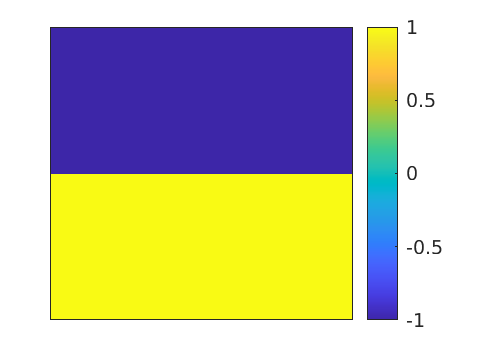
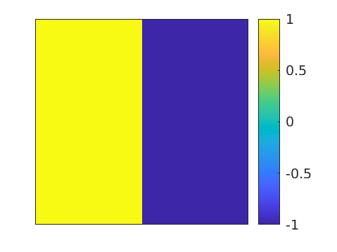
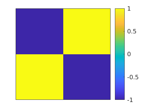
Figure 2. Three mother wavelets in 2d. From left to right: $\psi^{1},\psi^{2},\psi^{3}$.

Following Chkifa et al. [7], we assume that the conductivity $\sigma$ admits the parametrization

(6.1) $$\sigma(x,y):=\bar{\sigma}+c\sum_{l=0}^{\infty}2^{-\gamma l}\sum_{i=1}^{3}\sum_{k\in\{0,\dots,2^{l}-1\}^{2}}y_{l,k,i}\psi_{l,k}^{i}(x),$$

where $c,\gamma$ are positive constants. The upper and lower bounds for $\sigma$ are $\bar{\sigma}\pm c\sum_{l=0}^{\infty}2^{-\gamma l}$. We choose $\bar{\sigma}:=1.1$, $c:=0.3(1-2^{-\gamma})$ as in [7], so that the conductivity $\sigma$ always belongs to the bounded interval $[0.2,2.0]$. We convert the expansion (6.1) into the affine parametrization (2.9) by denoting

$$\psi_{j}:=c2^{-\gamma l}\psi_{l,k}^{i},y_{j}:=y_{l,k,i},$$

where $j=2^{2l}+3(2^{l}k_{1}+k_{2})+i-1$. It follows that $||\psi_{j}||_{L^{\infty}(D)}=O(j^{-\gamma/2})$. Hence, if $\gamma>2$, the decay rate in Assumption 3.1 is satisfied with $s=\gamma/2-1$.

6.1.2. Trigonometric prior

We consider a log-affine parametrization $\sigma(x)=e^{u(x)}$, where $u(x)$ is of the form

(6.2) $$u(x_{1},x_{2})=\sum_{j_{1},j_{2}\geq 0}y_{(j_{1},j_{2})}\frac{\eta}{(\tau^{2}+a^{2}\pi^{2}(j_{1}^{2}+j_{2}^{2}))^{\kappa}}\cos\left(\pi j_{1}x_{1}\right)\cos\left(\pi j_{2}x_{2}\right).$$

Here we choose $\eta=10^{-1}$, $\tau=3\cdot 10^{-1}$, $a=10^{-1.5}$ and $\kappa=5$; the random variables $y_{(j_{1},j_{2})}$ follow the uniform distribution in $[-1,1]$. This mimics the Kahunen-Loeve expansion of a Gaussian random variable of the Whittle-Matern type as considered in [15] for the EIT problem with a Gaussian prior, except that in our case the random variables $y_{j_{1},j_{2}}$ are uniformly distributed in $[-1,1]$. In this case, the corresponding Gaussian covariance is $\eta^{2}(\tau^{2}-a^{2}\Delta)^{-2\kappa}$, where $\Delta$ is the Laplace operator on $D=[0,1]^{2}$ with homogeneous Neumann boundary condition.

We cast (6.2) into the parametrization (2.10) by denoting

$$\psi_{j}:=\frac{\eta}{(\tau^{2}+a^{2}\pi^{2}(j_{1}^{2}+j_{2}^{2}))^{\kappa}}\cos\left(\pi j_{1}x_{1}\right)\cos\left(\pi j_{2}x_{2}\right),y_{j}:=y_{(j_{1},j_{2})},$$

where $j=0.5(j_{1}+j_{2})(j_{1}+j_{2}+1)+j_{2}+1$. It follows that $||\psi_{j}||_{L^{\infty}(D)}=O(j^{-\kappa})$.

6.2. Computational time of the sparse adaptive interpolation MCMC

The complexity of the adaptive interpolation algorithm has not been rigorously justified. We study numerically the complexity of Algorithm 2 with respect to the number $N$ of interpolating nodes, i.e. the cardinality of the lower set $\Lambda_{N}$. We measure the CPU time taken to perform the offline and online stages of sparse adaptive interpolation MCMC for various values of $J$ and $N$. In the online stage, we fix $M=10^{4}$.

The results are shown in Fig. 3 and Fig. 4. We observe that for fixed values of $J$, both the offline and online running times grow linearly in $N$. In addition, the slopes of the best-fit straight lines only increase moderately as $J$ increases.

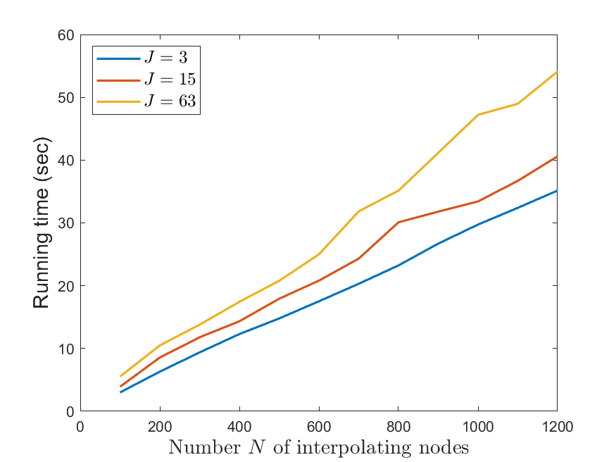
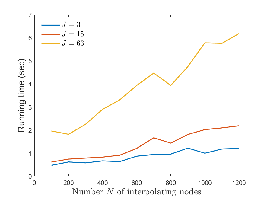
Figure 3. CPU time of the offline and online stages of sparse adaptive interpolation-MCMC using wavelet prior. Left: offline, right: online.

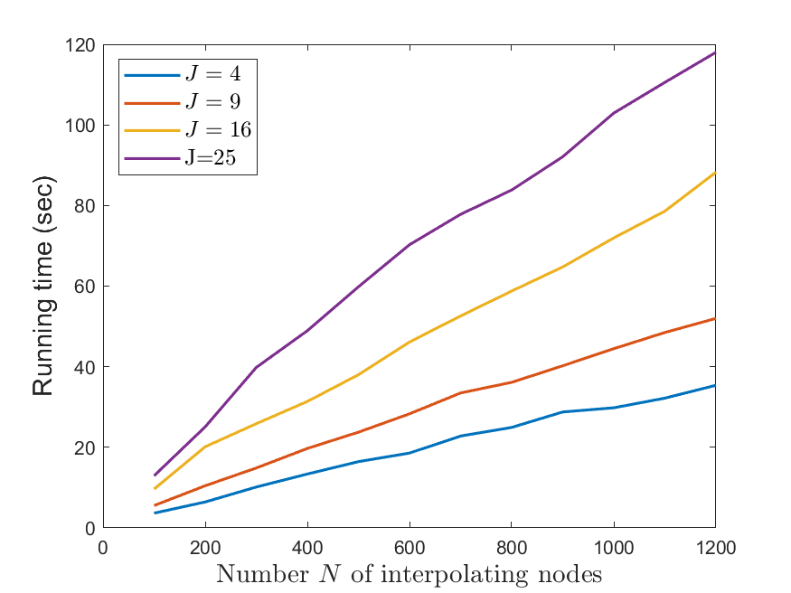
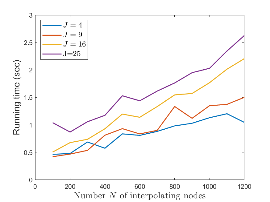
Figure 4. CPU time of the offline and online stages of sparse adaptive interpolation-MCMC using trigonometric prior. Left: offline, right: online.

6.3. Reconstruction

The initial state of the MCMC process is chosen randomly according to the uniform distribution. We use sparse adaptive interpolation with $N=5000$ interpolating nodes to approximate the forward map. We choose reflection random walk Metropolis (RRWM) as the MCMC sampling method, discarding the first $20\%$ samples as burn-in. The step size of RRWM is chosen to be $\beta:=0.001$. The acceptance probability is about 10%-30% in all experiments considered below. For the wavelet prior, to have a smoother visualization of the conductivity, we use bilinear interpolation to display the reconstructions.

First, we consider reconstructions using wavelet prior. We choose $\gamma=3$ in (6.1). The data are generated using $(y_{1},y_{2},y_{3})=(0.025,0.025,-0.025)$, $(y_{10},y_{11},y_{12})=(-0.8,-0.8,-0.8)$ and $y_{j}=0$ for other $j$’s. The true conductivity with this choice of $\boldsymbol{y}$ is displayed in the upper left of Fig. 5, with a square inclusion of lower conductivity.

To truncate expansion (6.1), we replace it with a finite summation where $l$ goes from $0$ to $L$ for some $L\geq 0$, namely

(6.3) $$\sigma^{J}(x,y):=\bar{\sigma}+c\sum_{l=0}^{L}2^{-\gamma l}\sum_{i=1}^{3}\sum_{k\in\{0,\dots,2^{l}-1\}^{2}}y_{l,k,i}\psi_{l,k}^{i}(x),$$

where $J=4^{L+1}-1$ is the total number of parameters. The resulting truncated approximation $\sigma^{J}$ is a piecewise constant function, which can be visualized by $2^{L+1}\times 2^{L+1}$ pixels.

In our first experiment, we use $L=1$ in (6.3) for reconstruction, corresponding to $J=15$ parameters. We use sparse adaptive interpolation MCMC with $M=10^{6}$ samples. The total time for adaptive selection of the index set $\Lambda$ and running MCMC is about 43 minutes. We then compare the reconstruction by sparse adaptive interpolation MCMC with the two reconstructions by plain MCMC: one with $10^{5}$ samples that takes 52 minutes to run, and one with $10^{6}$ samples that takes 10.5 hours. Fig. 5 demonstrates that the quality of reconstruction by sparse adaptive interpolation MCMC is comparable to that by plain MCMC with the same number of MCMC samples, with better contrast between the values of the conductivity inside the inclusion, and in the background. Sparse adaptive interpolation MCMC takes far less time than plain MCMC with the same number of samples, as we do not need to solve the forward problem with high accuracy at each sample. Comparing the recovered conductivity by sparse adaptive interpolation MCMC with $10^{6}$ samples to that obtained from the plain MCMC with $10^{5}$ samples, with a comparable running time, we find that the sparse adaptive interpolation MCMC provides a significantly better recovery, where the area of lower conductivity is smaller and is confined to the area of the original inclusion, and the background conductivity is closer to the original. If we use a finer FE mesh for reconstruction, we would expect more computational benefits from sparse adaptive interpolation MCMC.

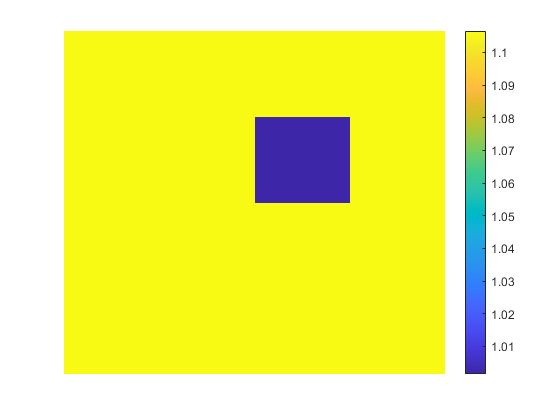
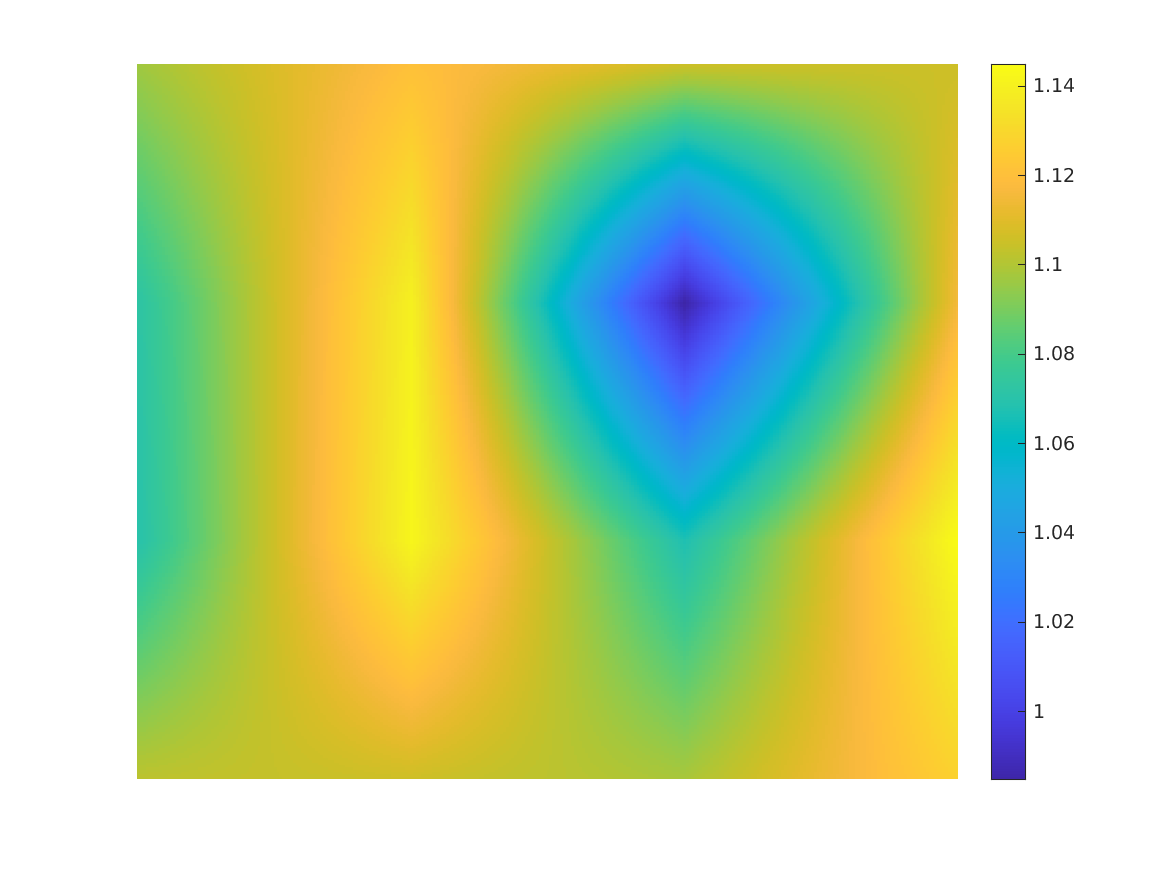
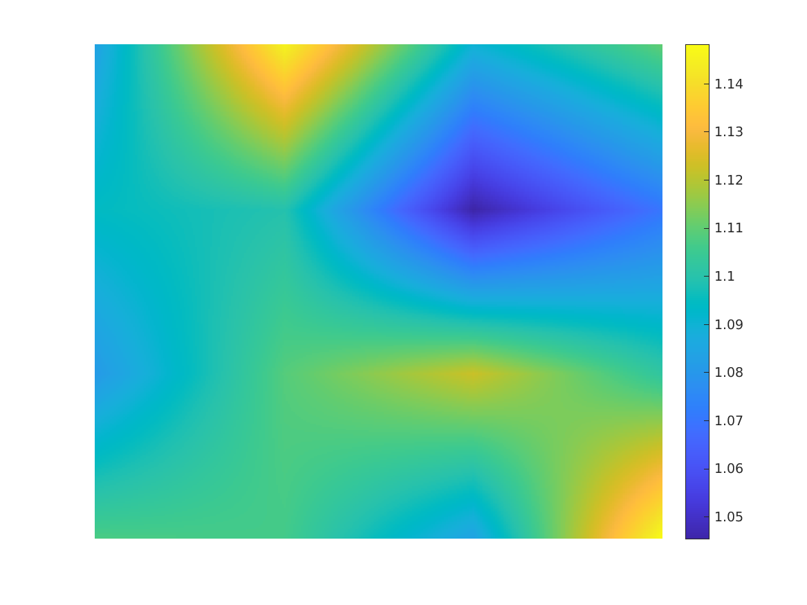
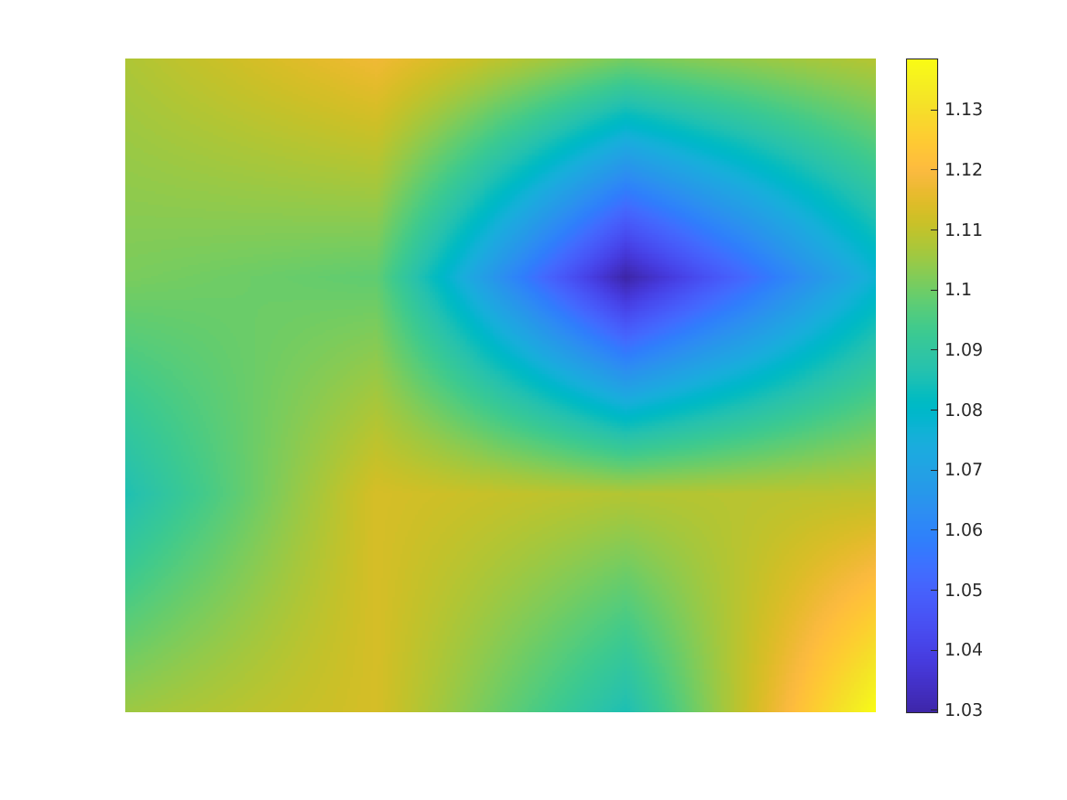
Figure 5. Reconstruction with wavelet prior using 16 pixels. Upper left: truth. Upper right: reconstruction by sparse adaptive interpolation MCMC with $10^{6}$ samples and $5000$ interpolating nodes. Lower left: reconstruction by plain MCMC with $10^{5}$ samples. Lower right: reconstruction by plain MCMC with $10^{6}$ samples.

Next, we compare the recovery for the conductivity produced by sparse adaptive interpolation MCMC, where the set of interpolating points $\Lambda$ is chosen by the adaptive algorithm, to that obtained by interpolation MCMC where the interpolating points are chosen isotropically, using a simple bound for the polynomial degree.

We consider a surrogate using interpolation with the following isotropic index set

$$Iso(15,5):=\{\nu\in\mathbb{N}_{0}^{15}:\nu_{1}+\dots+\nu_{15}\leq 5\}.$$

The index set $Iso(15,5)$ corresponds to the space of polynomials of 15 variables as in the numerical example above, but with degree at most 5. The cardinality of $Iso(15,5)$ is $\binom{15+5}{5}=15504$. The reconstruction by interpolation MCMC using $Iso(15,5)$ with the same number of MCMC samples, which is $10^{6}$, as in the previous numerical example, is shown in Fig. 6. Although the cardinality of $Iso(15,5)$ is significantly larger than that of $\Lambda$, i.e. here we have far more interpolating points, the reconstruction using $Iso(15,5)$ fails to capture the inclusion in the conductivity field. We provide a heuristic explanation as follows. Due to the decay rate of coefficients in the parametrization (6.3), the components $y_{1},y_{2},y_{3}$ contribute significantly more to $\sigma^{J}(x,y)$ than other components $y_{4},\dots,y_{15}$. Table 1 shows the maximum value and the average for each $\nu_{j}$ among the 5000 indices in the set $\Lambda$ constructed adaptively in the previous numerical example. We observe from Table 1 that most elements in the index set $\Lambda$ are placed in the directions corresponding to $y_{1},y_{2},y_{3}$. On the other hand, the average of each component $\nu_{j}$ of $\nu\in Iso(15,5)$ is $\frac{5}{15+1}=0.3125$. The isotropic approach treats all the parameters equally. As a result, the interpolant using $Iso(15,5)$ may not provide a good approximation of the forward map as the one using the anisotropic set $\Lambda$ constructed by the adaptive algorithm. This example shows clearly the advantage of the adaptive approach to construct the set of interpolating points over the isotropic approach.

	$\nu_{1}$	$\nu_{2}$	$\nu_{3}$	$\nu_{4}$	$\nu_{5}$	$\nu_{6}$	$\nu_{7}$	$\nu_{8}$	$\nu_{9}$	$\nu_{10}$	$\nu_{11}$	$\nu_{12}$	$\nu_{13}$	$\nu_{14}$	$\nu_{15}$
Max	8	8	8	3	3	3	3	3	3	3	3	3	3	3	3
Average	1.44	1.36	1.47	0.17	0.17	0.15	0.12	0.09	0.09	0.20	0.17	0.16	0.18	0.16	0.16

Table 1. The maximum and average of components of indices $\nu=(\nu_{1},\dots,\nu_{15})$ in the index set $\Lambda$, constructed by sparse adaptive interpolation, with $J=15$ in (6.3).

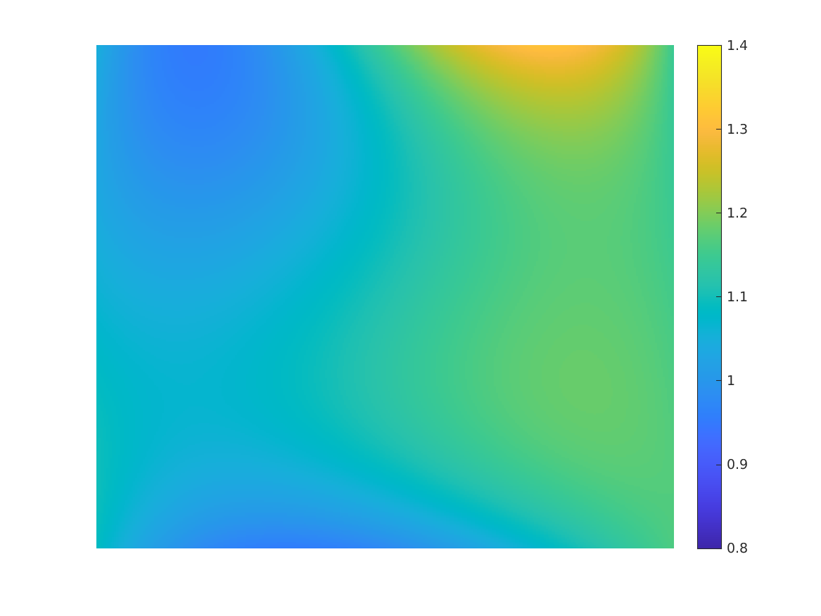
Figure 6. Reconstructions by sparse interpolation MCMC with the isotropic set $Iso(15,5)$ of cardinality 15504. Left: truth. Right: reconstruction using $Iso(15,5)$.

Next, we use the same reference conductivity for data generation and $L=2$ for reconstruction, corresponding to $J=63$ parameters. We use $M=10^{6}$ samples. Two constructions with $K=16$ and $K=64$ electrodes are displayed in Fig. 7, suggesting that increasing the number of parameters and the data size may enhance reconstruction quality: the panel on the right for the case of 64 electrodes shows better contrast in the values of the conductivity inside and outside of the inclusion.

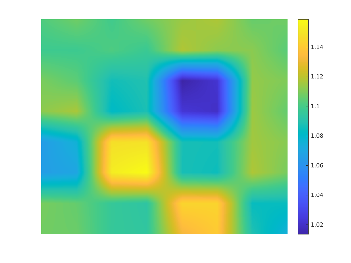
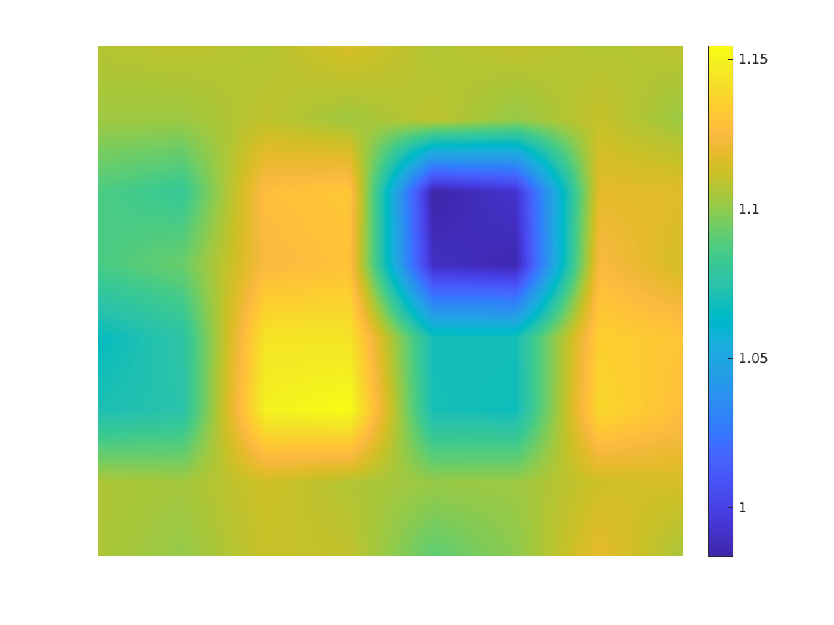
Figure 7. Reconstructions by sparse adaptive interpolation MCMC with wavelet prior using 64 pixels. Both plots use $10^{6}$ samples and $5000$ interpolating nodes. Left: 16 electrodes. Right: 64 electrodes.

Finally, we consider a reconstruction using trigonometric prior. In this experiment, we use $K=16$ electrodes. We replace the expansion (6.2) by a finite sum with $(j_{1},j_{2})\in\{0,1,\dots,7\}$, corresponding to $J=64$ parameters. We generate data by using a realization from the uniform distribution on $[-1,1]^{64}$ for the $y_{(j_{1},j_{2})}$’s. The target reference conductivity and the reconstruction by sparse adaptive interpolation MCMC with $M=10^{6}$ samples are shown in Fig. 8. This example illustrates the flexibility of the sparse adaptive interpolation MCMC process as it can be applied to different types of parametrization of the conductivity.

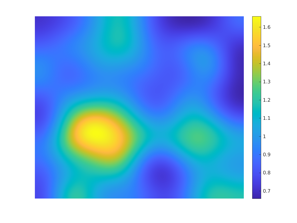
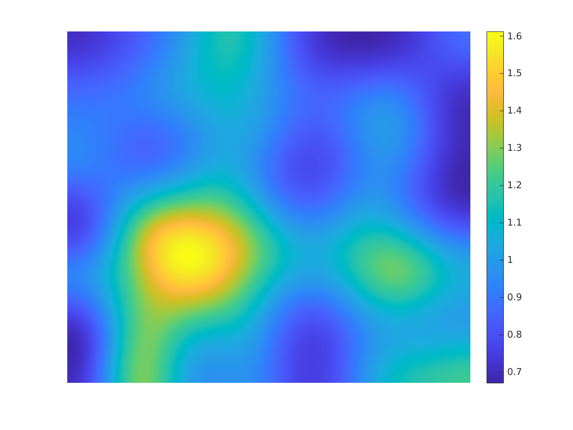
Figure 8. Reconstruction with trigonometric prior. Both plots use $10^{6}$ samples and $5000$ interpolating nodes. Left: truth. Right: reconstruction.

Appendix A Regularity and FE approximation of the forward solution

We derive in this appendix the FE error of the forward solver, uniformly with respect to $\boldsymbol{y}\in U$. We thus need to establish the regularity of the solution to the forward equation. We have the following estimate.

Lemma A.1.

For all $[(v,V)]\in\mathcal{H}^{1}$,

$$||\nabla v||_{L^{2}(D)}\leq||(v,V)||_{\mathcal{H}^{1}}.$$

Proof.

For every $c\in\mathbb{R}$,

$$||\nabla v||_{L^{2}(D)}=||\nabla(v-c)||_{L^{2}(D)}\leq||v-c||_{H^{1}(D)}\leq||v-c||_{H^{1}(D)}+|V-c{\bf 1}|.$$

Taking infimum with respect to $c\in\mathbb{R}$, we get the conclusion. ∎

In the following proposition, we show the uniform $H^{2}(D)$ regularity for the solution $v(\boldsymbol{y})$ of the forward equation, uniformly with respect to $\boldsymbol{y}\in U$.

Proposition A.2.

Under Assumption 3.3, for the solution $(v,V)$ to (2.4) $\|v(\boldsymbol{y})\|_{H^{2}(D)/{\mathbb{R}}}$ is uniformly bounded with respect to $\boldsymbol{y}\in U$.

Proof.

From (2.4),

$$\nu\cdot\sigma\nabla v=\zeta(V-v)\;\text{in }H^{-1/2}(\partial D),$$

(we omit the $\boldsymbol{y}$ dependence of $(v,V)$ and $\sigma$ for conciseness). Since $\sigma\in W^{1,\infty}(D)$ and $\sigma^{-}>0$, we have $1/\sigma\in W^{1,\infty}(D)$. It follows that $\frac{1}{\sigma}w\in H^{1}(D)$ for all $w\in H^{1}(D)$. Hence,

$$\nu\cdot\nabla v=\frac{\zeta(V-v)}{\sigma}.$$

Together with the identity $\nabla\cdot(\sigma\nabla v)=\nabla\sigma\cdot\nabla v+\sigma\Delta v$, we deduce that $v$ satisfies

$$\begin{cases}\Delta v=-\frac{\nabla\sigma\cdot\nabla v}{\sigma}\ \mbox{in }D,\\ \nu\cdot\nabla v=\frac{\zeta(V-v)}{\sigma}\ \mbox{on }\partial D.\end{cases}$$

As $V-v\in H^{1}(D)$, by the trace theorem $V-v\in H^{1/2}(\partial D)$. Since $\zeta\in W^{1,\infty}(\partial D)$, $\zeta(V-v)\in H^{1/2}(D)$. Since $D$ is convex, the solution $v_{0}$ of the problem

$$\begin{cases}\Delta v_{0}=-\frac{\nabla\sigma\cdot\nabla v}{\sigma}{\ \mbox{in }D,}\\ \nu\cdot\nabla v_{0}=0{\ \mbox{on }\partial D},\end{cases}$$

belongs to $H^{2}(D)/\mathbb{R}$, with

$$|v_{0}\|_{H^{2}(D)/\mathbb{R}}\leq C\|\frac{\nabla\sigma\cdot\nabla v}{\sigma}\|_{L^{2}(D)}\leq C\frac{||\sigma||_{W^{1,\infty}(D)}||\nabla v||_{L^{2}(D)}}{\sigma^{-}}\leq C|I|,$$

which is uniformly bounded with respect to $\boldsymbol{y}\in U$ (see, e.g, Grisvard [19] Theorem 3.2.1.3). Let $\zeta_{k}$ be the restriction of $\zeta$ on $E_{k}$, $\zeta_{k}$ is 0 outside $E_{k}$. Let $\partial D_{k}$ be the affine edge/surface of $\partial D$ that contains $E_{k}$ in $\mathbb{R}^{d}$, we extend $\zeta_{k}(V-v)/\sigma$ to 0 outside $E_{k}$. As $\bar{E}_{k}$ belongs to the interior of $\partial D_{k}$, we can find a function $\phi_{k}\in C^{\infty}_{0}(\mathbb{R}^{d})$ such that $\phi_{k}(x)=1$ for $x\in E_{k}$ and $(\partial D\setminus\partial D_{k})\cap{\rm supp}(\phi_{k})=\emptyset$. From the trace theorem, as $\partial D_{k}$ is linear, we can find a function $w^{\prime}_{k}\in H^{2}(D\cap{\rm supp}(\phi_{k}))$ such that $w_{k}^{\prime}=0$ on $\partial D_{k}$ and $\nu\cdot\nabla w_{k}^{\prime}=\zeta_{k}(V-v)/\sigma$ on $\partial D_{k}$ (which is 0 outside $E_{k}$). We note that $\|w_{k}^{\prime}\|_{H^{2}(D)}$ is uniformly bounded with respect to $\boldsymbol{y}$, namely

$$\|w_{k}^{\prime}\|_{H^{2}(D)}\leq C|\zeta|_{W^{1,\infty}(\partial D)}||V-v||_{H^{1}(D)}\leq C||(v,V)||_{\mathcal{H}^{1}}\leq C|I|.$$

Let $w_{k}=\phi_{k}w_{k}^{\prime}$, we find that $w_{k}\in H^{2}(D)$ such that on $\partial D_{k}$, $w_{k}=0$ and

$$\nu\cdot\nabla w_{k}=\nu\cdot(\nabla\phi_{k}w_{k}^{\prime}+\phi_{k}\nabla w_{k}^{\prime})=\phi_{k}\zeta_{k}(V-v)/\sigma$$

which equals 0 outside $E_{k}$ and $\zeta_{k}(V-v)/\sigma$ on $E_{k}$, as $\phi_{k}=1$ on $E_{k}$ and $\zeta_{k}=0$ outside $E_{k}$. Further, as other edges/surfaces of $\partial D$ are outside the support of $w_{k}$, we find that $\nu\cdot\nabla w_{k}=0$ on other edges/surfaces. We consider the problem

$$\begin{cases}\Delta v_{k}=0{\ \mbox{in }D,}\\ \nu\cdot\nabla v_{k}={\zeta_{k}(V-v)\over\sigma}=\nu\cdot\nabla w_{k}{\ \mbox{on }\partial D},\end{cases}$$

We note that $v_{k}-w_{k}$ is the solution of the homogeneous Neunman problem

$$\begin{cases}\Delta(v_{k}-w_{k})=-\Delta w_{k}\in L^{2}(D)\ \mbox{in }D,\\ \nu\cdot\nabla(v_{k}-w_{k})=0{\ \mbox{on }\partial D},\end{cases}$$

which is uniformly bounded in $H^{2}(D)/{\mathbb{R}}$ as $D$ is convex and $\Delta w_{k}$ is uniformly bounded in $L^{2}(D)$ for all $\boldsymbol{y}$ (Theorem 3.2.1.3 of [19]). By superposition, we obtain the desired result. ∎

Let $(v^{l},V^{l})$ be the FE approximation of $(v,V)$ with mesh size $O(2^{-l})$.

Lemma A.3.

Under Assumption 3.3,

(A.1) $$||(v,V)-(v^{l},V^{l})||_{\mathcal{H}^{1}}\leq C2^{-l}.$$

Proof.

By Cea’s lemma,

$$||(v,V)-(v^{l},V^{l})||_{\mathcal{H}^{1}}\leq C\frac{\max\{\sigma^{+},\zeta^{+}\}}{\min\{\sigma^{-},\zeta^{-}\}}\inf_{(w^{l},W^{l})\in\mathcal{V}^{l}}||(v,V)-(w^{l},W^{l})||_{\mathcal{H}^{1}}.$$

From the definition of $\mathcal{H}^{1}$-norm,

$$\inf_{(w^{l},W^{l})\in\mathcal{V}^{l}}||(v,V)-(w^{l},W^{l})||_{\mathcal{H}^{1}} =\inf_{w^{l}\in P^{l},W^{l}\in\mathbb{R}^{M},c\in\mathbb{R}}\left(||v-w^{l}-c||_{H^{1}(D)}+|V-W^{l}-c{\bf 1}|\right)$$

$$\leq\inf_{w^{l}\in P^{l},c\in\mathbb{R}}||(v-c)-w^{l}||_{H^{1}(D)}.$$

The desired estimate follows from Proposition A.2 and the approximation property of $P^{l}$, namely,

(A.2) $$\inf_{w^{l}\in P^{l}}||(v-c)-w^{l}||_{H^{1}(D)}\leq C2^{-l}||v-c||_{H^{2}(D)}.$$

∎

Proposition A.4.

Under Assumption 3.3,

$$|V-V^{l}|\leq C2^{-2l}.$$

Proof.

We follow the Aubin-Nitsche duality argument. For each $I^{*}\in\mathbb{R}^{K}_{\diamond}$, let $(v_{I^{*}},V_{I^{*}})\in\mathcal{H}^{1}$ be the solution to the problem

$$B((v_{I^{*}},V_{I^{*}}),(w,W))=I^{*}\cdot W\quad\forall(w,W)\in\mathcal{H}^{1}$$

and $(v_{I^{*}}^{l},V_{I^{*}}^{l})\in\mathcal{V}^{L}$ the solution to

$$B((v_{I^{*}}^{l},V_{I^{*}}^{l}),(w^{l},W^{l}))=I^{*}\cdot W^{l}\quad\forall(w^{l},W^{l})\in\mathcal{V}^{l}.$$

We have

$$|I^{*}\cdot(V-V^{l})| =|B((v_{I^{*}},V_{I^{*}}),(v-v^{l},V-V^{l}))|$$

$$=|B((v_{I^{*}}-v_{I^{*}}^{l},V_{I^{*}}-V_{I^{*}}^{l}),(v-v^{l},V-V^{l}))|$$

$$\leq C\max\{\sigma^{+},\zeta^{+}\}||(v_{I^{*}}-v_{I^{*}}^{l},V_{I^{*}}-V_{I^{*}}^{l})||_{\mathcal{H}^{1}}||(v-v^{l},V-V^{l})||_{\mathcal{H}^{1}}$$

$$\leq C2^{-2l}\|v_{I^{*}}\|_{H^{2}(D)/{\mathbb{R}}}\|v\|_{H^{2}(D)/{\mathbb{R}}}$$

where the third line follows from the boundedness of the bilinear form $B$ and the fourth line follows from (A.1). When $|I^{*}|=1$, from the proof Proposition A.2, $\|v_{I^{*}}\|_{H^{2}(D)/{\mathbb{R}}}$ is uniformly bounded with respect to $I^{*}$. Since $\mathbb{R}^{K}_{\diamond}$ is a closed subspace of $\mathbb{R}^{K}$, we obtain

$$|V-V^{l}|=\max_{{I^{*}}\in\mathbb{R}^{K}_{\diamond},|I^{*}|=1}|I^{*}\cdot(V-V^{l})|\leq C2^{-2l}.$$

∎

Appendix B Smoothened CEM with complex-valued conductivity

To establish the convergence rate in Proposition 4.3, following [7], we extend the range of the parameters to the complex plane, and consider a complex smoothened CEM problem. CEM problems with a complex-valued conductivity $\sigma$ have been studied extensive (see, e.g., [25] and references there in). Our aim is to establish the analyticity of the solution, and bound the coefficients of the Taylor expansion of the solution of the complex parametric problem in Appendix C. The solution belongs to the space

$$\mathcal{H}^{1}_{c}:=(H^{1}(D;\mathbb{C})\oplus\mathbb{C}^{K})/\mathbb{C}.$$

The corresponding variational formulation is

(B.1) $$B((v,V),(w,W);\sigma)=I\cdot\overline{W}\quad\forall\;(w,W)\in\mathcal{H}^{1}_{c},$$

where the sesquilinear form $B:\mathcal{H}^{1}_{c}\times\mathcal{H}^{1}_{c}\to\mathbb{C}$ is defined as

$$B((v,V),(w,W);\sigma)=\int_{D}\sigma\nabla v\cdot\nabla\overline{w}dx+\int_{\partial D}\zeta(V-v)(\overline{W}-\overline{w})dS.$$

We denote by $\mathcal{A}(D)$ the class of $\sigma\in L^{\infty}(D;\mathbb{C})$ such that there exist $\sigma^{+},\sigma^{-}>0$ satisfying

(B.2) $$\sigma^{-}\leq\operatorname{Re}(\sigma(x))\leq|\sigma(x)|\leq\sigma^{+}\;\forall x\in D.$$

To simplify the notation, we use $\mathcal{H}^{1}$ for $\mathcal{H}^{1}_{c}$. It should not be confused with the real vector space counterpart. From Lemma 2.1 in [25], provided that (B.2) holds, the sesquilinear form $B$ is bounded and coercive with

$$\operatorname{Re}B((v,V),(v,V))\geq C\min\{\sigma^{-},\zeta^{-}\}||(v,V)||_{\mathcal{H}^{1}}.$$

In the quotient space $\mathcal{H}^{1}$, we choose the representative $(v,V)$ such that $V$ belongs to

$$\mathbb{C}^{K}_{\diamond}:=\{U\in\mathbb{C}^{K}:U_{1}+\dots+U_{K}=0\}.$$

As in Lemmas 2.1 and A.1, we can show that $|V|\leq||(v,V)||_{\mathcal{H}^{1}}$ and $||\nabla v||_{L^{2}(D)}\leq||(v,V)||_{\mathcal{H}^{1}}$. Hence

$$|V|\leq C\frac{|I|}{\min\{\sigma^{-},\zeta^{-}\}}.$$

The piecewise linear FE approximation $(v^{l},V^{l})$ with mesh size $O(2^{-l})$ belongs to the space $\mathcal{V}^{l}_{C}:=(P^{l}\oplus\mathbb{C}^{K})/\mathbb{C}$. We have

(B.3) $$|V^{l}|\leq C\frac{|I|}{\min\{\sigma^{-},\zeta^{-}\}}.$$

We now show the continuous dependence of the solution to the forward problem on the conductivity.

Lemma B.1.

Let $\sigma_{1},\sigma_{2}$ belong to $\mathcal{A}(D)$ with bounds $\sigma^{-}$ and $\sigma^{+}$ in (B.2). We then have

$$||(v(\sigma_{1})-v(\sigma_{2}),V(\sigma_{1})-V(\sigma_{2}))||_{\mathcal{H}^{1}}\leq C\|\sigma_{1}-\sigma_{2}\|_{L^{\infty}(D)},$$

where $C$ depends on $\sigma^{-}$ and $\sigma^{+}$.

Proof.

For any $\sigma\in\mathcal{A}(D)$, denote $\mathcal{M}(\sigma):=((v(\sigma),V(\sigma)))$. We show that for $\sigma_{1},\sigma_{2}\in\mathcal{A}(D)$,

(B.4) $$||\mathcal{M}(\sigma_{1})-\mathcal{M}(\sigma_{2})||_{\mathcal{H}^{1}}\leq C\frac{||\sigma_{1}-\sigma_{2}||_{L^{\infty}(D)}||\mathcal{M}(\sigma_{2})||_{\mathcal{H}^{1}}}{\min\{\inf_{x\in D}\operatorname{Re}(\sigma_{1}(x)),\zeta^{-}\}}.$$

Denote $(v_{j},V_{j})=(v(\sigma_{j}),V(\sigma_{j})),j=1,2$. Since for all $(w,W)\in\mathcal{H}^{1}$,

$$B((v_{1},V_{1}),(w,W);\sigma_{1})=I\cdot\overline{W}=B((v_{2},V_{2}),(w,W);\sigma_{2}),$$

we have

$$0 =B((v_{1},V_{1}),(w,W);\sigma_{1}))-B((v_{2},V_{2}),(w,W);\sigma_{1})+B((v_{2},V_{2}),(w,W);\sigma_{1})-B((v_{2},V_{2}),(w,W);\sigma_{2})$$

$$=\int_{D}\sigma_{1}\nabla(v_{1}-v_{2})\cdot\nabla\overline{w}dx+\int_{\partial D}\zeta((V_{1}-V_{2})-(v_{1}-v_{2}))(\overline{W}-\overline{w})dS+\int_{D}(\sigma_{1}-\sigma_{2})\nabla v_{2}\cdot\nabla\overline{w}dx.$$

Let $(w,W)=(v_{1}-v_{2},V_{1}-V_{2})$. Then

$$\int_{D}\operatorname{Re}(\sigma_{1})|\nabla(v_{1}-v_{2})|^{2}dx+\int_{\partial D}\zeta|(V_{1}-V_{2})-(v_{1}-v_{2})|^{2}dS\leq\int_{D}|\sigma_{1}-\sigma_{2}||\nabla v_{2}\cdot\nabla(\overline{v_{1}-v_{2}})|dx.$$

From estimate (9) in [25], we deduce

$$||(v_{1}-v_{2},V_{1}-V_{2})||_{\mathcal{H}^{1}}^{2}\leq C(||\nabla(v_{1}-v_{2})||^{2}_{L^{2}(D)}+||(V_{1}-V_{2})-(v_{1}-v_{2})||_{L^{2}(\partial D)}).$$

From $\eqref{zeta_lower_bound}$ and the assumption that $\operatorname{Re}(\sigma_{1})$ is bounded below,

$$||(v_{1}-v_{2},V_{1}-V_{2})||_{\mathcal{H}^{1}}^{2}\leq C_{\sigma_{1}}\left(\int_{D}\operatorname{Re}(\sigma_{1})|\nabla(v_{1}-v_{2})|^{2}dx+\int_{\partial D}\zeta((V_{1}-V_{2})-(v_{1}-v_{2}))^{2}dS\right),$$

where $C_{\sigma_{1}}=\frac{C}{\min\{\inf_{x\in D}\operatorname{Re}(\sigma_{1}(x)),\zeta^{-}\}}$. Hence

$$||(v_{1}-v_{2},V_{1}-V_{2})||_{\mathcal{H}^{1}}^{2} \leq C_{\sigma_{1}}\left(\int_{D}|\sigma_{1}-\sigma_{2}|^{2}|\nabla v_{2}|^{2}dx\right)^{1/2}||\nabla(v_{1}-v_{2})||_{L^{2}(D)}$$

$$\leq C_{\sigma_{1}}||\sigma_{1}-\sigma_{2}||_{L^{\infty}(D)}||\nabla v_{2}||_{L^{2}(D)}||(v_{1}-v_{2},V_{1}-V_{2})||_{\mathcal{H}^{1}}$$

$$\leq C_{\sigma_{1}}||\sigma_{1}-\sigma_{2}||_{L^{\infty}(D)}||(v_{2},V_{2})||_{\mathcal{H}^{1}}||(v_{1}-v_{2},V_{1}-V_{2})||_{\mathcal{H}^{1}}.$$

We then get (B.4). From the uniform boundedness of $\|\mathcal{M}(\sigma)\|_{\mathcal{H}^{1}}$ for all $\sigma\in A(D)$, we get the conclusion.

∎

Appendix C Error estimates

C.1. Truncation error

Proof of Proposition 3.2.

The normalizing constants of $\mu^{\delta}$ and $\mu^{J,\delta}$ in (2.14) and (3.2) are

$$Z(\delta):=\int_{U}\exp(-\Phi(\boldsymbol{y};\delta))d\mu_{0}(\boldsymbol{y});\quad Z^{J}(\delta):=\int_{U}\exp(-\Phi^{J}(\boldsymbol{y};\delta))d\mu_{0}(\boldsymbol{y}).$$

From the definition of Hellinger distance,

$$2d_{Hell}(\mu^{\delta},\mu^{J,\delta})^{2} =\int_{U}\left(Z(\delta)^{-1/2}\exp(-\frac{1}{2}\Phi(y;\delta))-(Z^{J}(\delta))^{-1/2}\exp(-\frac{1}{2}\Phi^{J}(y;\delta))\right)^{2}d\mu_{0}(\boldsymbol{y})$$

$$\leq I_{1}+I_{2},$$

where

$$I_{1} =\frac{1}{Z(\delta)}\int_{U}\left(\exp(-\frac{1}{2}\Phi(\boldsymbol{y};\delta))-\exp(-\frac{1}{2}\Phi^{J}(\boldsymbol{y};\delta))\right)^{2}d\mu_{0}(\boldsymbol{y})$$

$$I_{2} =|Z(\delta)^{-1/2}-Z^{J}(\delta)^{-1/2}|^{2}Z^{J}(\delta).$$

From (2.15) and (3.5), $Z(\delta)$ and $Z^{J}(\delta)$ are uniformly bounded below by a positive constant. Hence

$$I_{2} \leq C|Z(\delta)-Z^{J}(\delta)|^{2}$$

$$\leq C\int_{U}|\exp(-\Phi(\boldsymbol{y};\delta))-\exp(-\Phi^{J}(\boldsymbol{y};\delta)|^{2}d\mu_{0}(\boldsymbol{y}).$$

By the inequality $|e^{-a}-e^{-b}|\leq|a-b|$ for $a,b\geq 0$, we deduce

$$I_{1},I_{2}\leq C\left(\sup_{\boldsymbol{y}\in U}|\Phi(\boldsymbol{y};\delta)-\Phi^{J}(\boldsymbol{y};\delta)|\right)^{2}.$$

Together with (3.6), we arrive at the conclusion. ∎

C.2. Interpolation error

The idea of using analyticity to obtain convergence rates of polynomial approximation of parametric PDEs has been exploited in [11] and applied to interpolation in [7, 8]. As the results in these papers are formulated for elliptic PDEs with Dirichlet boundary conditions, minor modifications are needed to apply to EIT.

We begin with the analyticity of the parametric forward solutions. The parametrization of $\sigma$ can be extended to the complex plane by defining

$$\sigma^{J}(x,\xi):=\bar{\sigma}(x)+\sum_{j=1}^{J}\xi_{j}\psi_{j}(x),\quad\xi\in\mathbb{C}^{J}.$$

For any sequence of positive numbers $\rho=(\rho_{1},\dots,\rho_{J})$, let $\mathcal{D}^{J}_{\rho}:=\{\xi\in\mathbb{C}^{J}:|\xi_{j}|\leq\rho_{j}\;\forall j\}$. We note that $\mathcal{D}^{J}_{\rho}$ contains $U_{J}=[-1,1]^{J}$ when $\rho_{j}>1\;\forall j$. If

(C.1) $$\sum_{j=1}^{J}\rho_{j}|\psi_{j}(x)|\leq\bar{\sigma}(x)-\sigma^{-}/2,$$

then the polydisc $\mathcal{D}^{J}_{\rho}$ is contained in the set

$$\mathcal{A}_{J}:=\{\xi\in\mathbb{C}^{J}:\sigma^{-}/2\leq\operatorname{Re}(\sigma^{J}(x,\xi))\leq|\sigma^{J}(x,\xi)|\leq 2\sigma^{+}\;\forall x\in D\}.$$

It follows from Appendix B that $\mathcal{G}^{J,l}(z)$ is well-defined for all $\xi\in\mathcal{A}_{J}$.

Lemma C.1.

The function $\xi\mapsto\mathcal{G}^{J,l}(\xi)$ is holomorphic on $\mathcal{A}_{J}$.

Proof.

It suffices to show that for any $k=1,\dots,K-1$, the map $\xi\mapsto V^{l,(k)}(\sigma^{J}(\cdot,\xi))$ for the FE solution admits complex partial derivatives at every point in $\mathcal{A}_{J}$. To ease notation, we drop the superscript $(l,k)$ and denote each of these maps by $V$ and their corresponding potential by $v$. Let $\{e_{1},\dots,e_{J}\}$ be the canonical basis in $\mathbb{R}^{J}$. Fix $j\in\{1,\dots,J\}$ and $\xi\in\mathcal{A}_{J}$. For $h\in\mathbb{C}\backslash\{0\}$ with $|h|$ small enough such that $(v(\xi+he_{j}),V(\xi+he_{j}))$ is well-defined, let

$$v_{h}(\xi) :=\frac{v(\xi+he_{j})-v(\xi)}{h};$$

$$V_{h}(\xi) :=\frac{V(\xi+he_{j})-V(\xi)}{h}.$$

Note that $(v(\xi),V(\xi))$ and $(v(\xi+he_{j}),V(\xi+he_{j}))$ satisfy the variational problems

$$B((v(\xi),V(\xi)),(w^{l},W^{l});\sigma^{J}(\xi))=I\cdot W^{l}\quad\forall(w^{l},W^{l})\in\mathcal{V}^{l}$$

and

$$B((v(\xi),V(\xi+he_{j})),(w^{l},W^{l});\sigma^{J}(\xi+he_{j}))=I\cdot W^{l}\quad\forall(w^{l},W^{l})\in\mathcal{V}^{l}.$$

Subtracting these equalities, we find that for all $(w^{l},W^{l})\in\mathcal{V}^{l}$,

$$0 =\int_{D}[\sigma(x,\xi+he_{j})-\sigma(x,\xi)]\nabla v(\xi+he_{j})\cdot\nabla\overline{w^{l}}(x)dx+\int_{D}\sigma(x,\xi)[\nabla v(\xi+he_{j})-\nabla v(\xi)]\cdot\nabla\overline{w^{l}}(x)$$

$$+\int_{\partial D}\zeta[V(\xi+he_{j})-V(\xi)-v(\xi+he_{j})+v(\xi)]\overline{W^{l}-w^{l}}dS$$

$$=\int_{D}h\psi_{j}(x)\nabla v(x,\xi+he_{j})\cdot\nabla\overline{w^{l}}(x)dx+\int_{D}\sigma(x,\xi)h\nabla v_{h}(\xi)\cdot\nabla\overline{w^{l}}(x)dx$$

$$+\int_{\partial D}\zeta h[V_{h}(\xi)-v_{h}(\xi)]\overline{W^{l}-w^{l}}dS$$

$$=hB((v_{h},V_{h}),(w^{l},W^{l});\sigma(\xi))+h\int_{D}\psi_{j}(x)\nabla v(x,\xi+he_{j})\cdot\nabla\overline{w^{l}}(x)dx.$$

It follows that $(v_{h},V_{h})$ satisfies

(C.2) $$B((v_{h},V_{h}),(w^{l},W^{l});\sigma(\xi))=-\int_{D}\psi_{j}(x)\nabla v(x,\xi+he_{j})\cdot\nabla\overline{w^{l}}(x)dx.$$

For each $h\in\mathbb{C}$ and $(w,W)\in\mathcal{H}^{1}$, let

$$L_{h}((w,W)):=-\int_{D}\psi_{j}(x)\nabla v(x,\xi+he_{j})\cdot\nabla\overline{w^{l}}(x)dx.$$

Then $L_{h}$ is a bounded linear functional on $\mathcal{H}^{1}$ because

$$|L_{h}((w,W))|\leq||\psi_{j}||_{L^{\infty}(D)}||v(\cdot,\xi+he_{j})||_{H^{1}(D)}||w||_{H^{1}(D)}.$$

Let $(v_{0},V_{0})$ be the unique solution to the variational problem

$$B((v_{0},V_{0}),(w^{l},W^{l});\sigma(z))=L_{0}((w^{l},W^{l}))\;\forall(w^{l},W^{l})\in\mathcal{V}^{l}.$$

For all $(w,w)\in\mathcal{H}^{1}$, we have

$$|L_{h}((w,W))-L_{0}((w,W))| =|\int_{D}\psi_{j}(x)[\nabla v(x,\xi+he_{j})-v(x,\xi)]\cdot\nabla\overline{w}(x)dx|$$

$$\leq||\psi_{j}||_{L^{\infty}(D)}||\nabla[v(\xi+he_{j})-v(\xi)]||_{L^{2}(D)}||\nabla w||_{L^{2}(D)}.$$

From Lemma A.1 and Lemma B.1, we deduce

$$\lim_{h\to 0}||\nabla[v(\xi+he_{j})-v(z)]||_{L^{2}(D)}=0.$$

Since $L_{h}((w,W))\to L_{0}((w,W))$ for every $(w,W)\in\mathcal{H}^{1}$, it follows that $(v_{h},V_{h})$ converges to $(v_{0},V_{0})$ in $\mathcal{H}^{1}$. From Lemma 2.1, we have $\lim_{h\to 0}|V_{h}-V_{0}|=0$. Therefore $\partial_{z_{j}}V(z)=V_{0}$. ∎

Lemma C.2.

The Taylor series $\sum_{\nu\in\mathbb{N}_{0}^{J}}t_{\nu,J,l}y_{1}^{\nu_{1}}\dots y_{J}^{\nu_{J}}$ converges unconditionally to $\mathcal{G}^{J,l}$ on $U_{J}$, where

$$t_{\nu,J,l}:=\frac{1}{\nu!}\partial^{\nu}\mathcal{G}^{J,l}(0).$$

Proof.

From (2.12) we have

$$\sum_{j=1}^{J}|\psi_{j}(x)|\leq\bar{\sigma}(x)-\sigma^{-}.$$

Hence there exists a sequence $\rho\in\mathbb{R}^{J}$ such that $\rho_{j}>1$ for all $j$ and (C.1) holds. This implies that the Taylor series of $\mathcal{G}^{J,l}(\xi)$ converges unconditionally for all $\xi$ in the interior of $\mathcal{D}^{J}_{\rho}$, which contains $U_{J}$. ∎

Lemma C.3.

For any positive sequence $\rho\in\mathbb{R}^{J}$ satisfying (C.1), there is a constant $C$ independent of $\nu,J,l$ such that

$$|t_{\nu,J,l}|\leq C\rho^{-\nu}.$$

Proof.

Since the map $z\mapsto\mathcal{G}^{J,l}(z)$ is holomorphic on $\mathcal{D}_{\rho}^{J}$, the Cauchy’s integral theorem (see e.g., Theorem 2.2.6 in [23]) gives

$$t_{\nu,J,l}=\frac{1}{(2\pi i)^{J}}\int_{|\xi_{1}|=\rho_{1}}\dots\int_{|\xi_{J}|=\rho_{J}}\frac{\mathcal{G}^{J,l}(\xi_{1},\dots,\xi_{J})}{\xi_{1}^{\nu_{1}+1}\dots\xi_{J}^{\nu_{J}+1}}.$$

From (B.3), we deduce that $\mathcal{G}^{J,l}(\xi)$ is uniformly bounded for all $J,l\in\mathbb{N},\xi\in\mathcal{D}^{J}_{\rho}$. Hence the desired estimate follows.

∎

Proof of Proposition 4.3.

Using Lemma 4.2 in [7] and Lemma C.2, the interpolation error in approximating $\mathcal{G}^{J,l}$ can be linked to the decay of its Taylor coefficients, namely

(C.3) $$\sup_{y\in U_{J}}|\mathcal{G}^{J,l}(y)-I_{\Lambda}\mathcal{G}^{J,l}(y)|\leq 2\sum_{\nu\notin\Lambda}p_{\nu,J}(\theta)|t_{\nu,J,l}|,$$

where $p_{\nu,J}(\theta):=\prod_{j=1}^{J}(1+\nu_{j})^{\theta+1}$. With (C.3) and Lemma C.3, we can proceed as in the proof of Theorem 4.3 in [7] to complete the proof of the theorem. ∎

Remark C.4.

For log-affine parametrization (2.10), we can perform error analysis using results in [8]. The Taylor series of $\mathcal{G}^{J,l}$ should be replaced by a Legendre series, and a similar interpolation error of order $(N+1)^{-s}$ could be obtained.

C.3. Monte Carlo error

To analyze the MCMC error, we use the concept of ‘second largest eigenvalue’ for Markov operators. We follow the literature, e.g., [37].

For the proposal $Q^{J}$ in (5.1), we define the ’second largest eigenvalue’ with respect to $Q^{J}$ and $\mu_{0}^{J}$ as follows. The corresponding Markov operator $\mathcal{Q}^{J}$ acting on $L^{2}(U_{J},\mathbb{R};\mu_{0}^{J})$ is defined by

$$\mathcal{Q}^{J}f(\boldsymbol{y}):=\int_{U_{J}}f(\boldsymbol{s})Q^{J}(y,d\boldsymbol{s}).$$

Since $Q^{J}$ is reversible with respect to $\mu_{0}^{J}$, the linear operator $\mathcal{Q}^{J}$ is self-adjoint and its spectrum lies in the interval $[-1,1]$. Moreover, $1$ is the largest eigenvalue of $\mathcal{Q}^{J}$ since $\mathcal{Q}^{J}c=c$ for any constant functional $c$. Let $L_{0}^{2}(\mu_{0}^{J})$ be the space of measurable functions $f:U_{J}\to\mathbb{R}$ such that

$$\int_{U_{J}}f(\boldsymbol{y})d\mu_{0}^{J}(\boldsymbol{y})=0;\quad\int_{U_{J}}[f(\boldsymbol{y})]^{2}d\mu_{0}^{J}(\boldsymbol{y})=1.$$

The ‘second largest eigenvalue’ $\lambda_{(2)}^{Q^{J},\mu_{0}^{J}}$ is defined as

(C.4) $$\lambda_{(2)}^{Q^{J},\mu_{0}^{J}}:=\sup_{f\in L_{0}^{2}(\mu_{0}^{J})}\int_{U_{J}}[\mathcal{Q}^{J}f(\boldsymbol{y})]f(\boldsymbol{y})d\mu_{0}^{J}(\boldsymbol{y}).$$

Equivalently, $\lambda_{(2)}^{Q^{J},\mu_{0}^{J}}$ can be interpreted as the least upper bound of the spectrum of the restriction of $\mathcal{Q}^{J}$ to the orthogonal complement of the space of constant functionals [37].

Let $K^{J,l,N}$ be the transition kernel with proposal $Q^{J}$ and acceptance probability $\alpha^{J,l,N}$ in (5.2). Since $K^{J,l,N}$ is reversible with respect to the approximated posterior distribution $\mu^{J,l,N,\delta}$, we can define the ‘second largest eigenvalue’ $\lambda_{(2)}^{K^{J,l,N},\mu^{J,l,N,\delta}}$ in a similar manner as (C.4) when $Q^{J}$ and $\mu_{0}^{J}$ are replaced by $K^{J,l,N}$ and $\mu^{J,l,N,\delta}$, respectively.

We assume that the second largest eigenvalue of $Q^{J}$ is uniformly bounded by a constant strictly less than $1$.

Assumption C.5.

$\sup_{J}\lambda_{(2)}^{Q^{J},\mu_{0}^{J}}<1$.

This assumption can be verified for the Independence Sampler and Reflection Random Walk Metropolis sampling methods. For Independence Sampler, it is clear from (C.4) that $\lambda_{(2)}^{Q_{IS}^{J},\mu_{0}^{J}}=0$ for all $J$. For the Reflection Random Warl Metropolis, the above assumption is verified in [42] in the case $\mu_{0}^{J}$ is the uniform prior on $U_{J}$.

Lemma C.6.

Under Assumption C.5, there exists a positive constant $\lambda_{(2)}<1$ such that

$$\sup_{J,l,N}\lambda_{(2)}^{K^{J,l,N},\mu^{J,l,N,\delta}}\leq\lambda_{(2)}.$$

Proof.

Since $|\mathcal{G}^{J,l,N}(\boldsymbol{y})|$ is uniformly bounded, there exists a constant $c>0$ independent of $J,l,N$ such that for all $\boldsymbol{y}\in U_{J}$,

$$0<c\leq\exp(-\Phi^{J,l,N}(\boldsymbol{y};\delta))\leq 1.$$

Theorem 3.3 in [42] implies that for any $J,l,N$,

$$1-\lambda_{(2)}^{K^{J,l,N},\mu^{J,l,N,\delta}}\geq c^{4}(1-\lambda_{(2)}^{Q^{J},\mu_{0}^{J}}).$$

By Assumption C.5, the RHS is uniformly bounded below by a positive constant. ∎

For each probability distribution $\mu$ on $U_{J}$, we denote by $\mathcal{E}^{\mu,J,l,N}$ the expectation taken with respect to the joint distribution of the Markov chain $(u^{(i)})_{i=1}^{\infty}$ with transition kernel $K^{J,l,N}$ and initial distribution $\mu$. From Corollary 3.27 in [37] and Lemma C.6, we deduce that if Assumption C.5 holds then for any function $g:U_{J}\to\mathbb{R}$ such that $\sup_{y\in U_{J}}|g(\boldsymbol{y})|\leq 1$,

(C.5) $$\left(\mathcal{E}^{\mu^{J,l,N,\delta},J,l,N}\left[\left|E^{\mu^{J,l,N,\delta}}[g]-E_{M}^{\mu^{J,l,N,\delta}}[g]\right|^{2}\right]\right)^{1/2}\leq\sqrt{\frac{2}{1-\lambda_{(2)}}}M^{-1/2}.$$

Theorem C.7.

Under Assumptions 3.1, 3.3, 4.2, C.5, there exists a nested sequence of lower sets $(\Lambda_{N})_{N\geq 1}$ such that $\#(\Lambda_{N})=N$ and

(C.6) $$\left(\mathcal{E}^{\mu_{0}^{J},J,l,N}\left[\left\|E^{\mu^{J,\delta}}[\sigma^{J}]-E_{M}^{\mu^{J,l,N,\delta}}[\sigma^{J}]\right\|_{L^{\infty}(D)}^{2}\right]\right)^{1/2}\leq C(2^{-2l}+N^{-s}+M^{-1/2}),$$

where $C$ is a constant independent of $J,l,N,M$.

Proof.

As $\sup_{\boldsymbol{y}\in U_{J}}||\sigma^{J}(\cdot,\boldsymbol{y})||_{L^{\infty}(D)}\leq\sigma^{+}$, applying Lemma 21 in [14] yields

$$||E^{\mu^{J,\delta}}[\sigma^{J}]-E^{\mu^{J,l,N\delta}}[\sigma^{J}]||_{L^{\infty}(D)}\leq 2\sqrt{2}\sigma^{+}d_{Hell}(\mu^{J,l,N,\delta},\mu^{J,\delta}).$$

Combining with the Hellinger distance estimate in Proposition 4.4, we have

(C.7) $$||E^{\mu^{J,\delta}}[\sigma^{J}]-E^{\mu^{J,l,N\delta}}[\sigma^{J}]||_{L^{\infty}(D)}\leq C_{1}(2^{-2l}+N^{-s}),$$

for some constant $C_{1}$ independent of $J,l,N$.

Due to the linearity of expectations,

$$E^{J,l,N,\delta}[\sigma^{J}]-E^{\mu^{J,l,N,\delta}}_{M}[\sigma^{J}]=\sum_{j=1}^{J}\psi_{j}(x)\left[E^{J,l,N,\delta}[y_{j}]-E^{\mu^{J,l,N,\delta}}_{M}[y_{j}]\right],$$

Applying (C.5) for $g=y_{j}$ and using the triangle inequality, we deduce

$$\left(\mathcal{E}^{\mu^{J,l,N,\delta},J,l,N}\left[\left|E^{\mu^{J,l,N,\delta}}[\sigma^{J}]-E_{M}^{\mu^{J,l,N,\delta}}[\sigma^{J}]\right|^{2}\right]\right)^{1/2}\leq\sqrt{\frac{2}{1-\lambda_{(2)}}}M^{-1/2}\sum_{j=1}^{J}||\psi_{j}||_{L^{\infty}(D)}.$$

From Assumption 3.1 about the decay rate of $(||\psi_{j}||_{L^{\infty}(D)})_{j\geq 1}$, we have

$$\sum_{j=1}^{J}||\psi_{j}||_{L^{\infty}(D)}\leq\sum_{j=1}^{\infty}||\psi_{j}||_{L^{\infty}(D)}<\infty.$$

On the other hand, note that

$$\frac{d\mu_{0}^{J}}{d\mu^{J,l,N,\delta}}=Z^{J,l,N}(\delta)\exp(\Phi^{J,l,N}(\boldsymbol{y};\delta))\leq\exp(\Phi^{J,l,N}(\boldsymbol{y};\delta)).$$

Since $|\mathcal{G}^{J,l,N}(\boldsymbol{y})|$ is uniformly bounded, the Radon-Nikodym derivative of $\mu_{0}^{J}$ with respect to $\mu^{J,l,N,\delta}$ is uniformly bounded. Hence, there exists a constant $C_{2}$ independent of $J,l,N,M$ such that

(C.8) $$\left(\mathcal{E}^{\mu_{0}^{J},J,l,N}\left[\left|E^{\mu^{J,l,N,\delta}}[\sigma^{J}]-E_{M}^{\mu^{J,l,N,\delta}}[\sigma^{J}]\right|^{2}\right]\right)^{1/2}\leq C_{2}M^{-1/2}.$$

The proof is completed by combining (C.7) and (C.8). ∎

Proof of Theorem 5.1.

Proposition 3.2 and Lemma 21 in [14] imply that

$$||E^{\mu^{\delta}}[\sigma]-E^{\mu^{J,\delta}}[\sigma]||_{L^{\infty}(D)}\leq 2\sqrt{2}\sigma^{+}d_{Hell}(\mu^{\delta},\mu^{J,\delta})\leq CJ^{-s}.$$

On the other hand, from (3.4),

$$||E^{\mu^{J,\delta}}[\sigma]-E^{\mu^{J,\delta}}[\sigma^{J}]||_{L^{\infty}(D)}\leq CJ^{-s}.$$

Hence, by the triangle inequality,

(C.9) $$||E^{\mu^{\delta}}[\sigma]-E^{\mu^{J,\delta}}[\sigma^{J}]||_{L^{\infty}(D)}\leq CJ^{-s}.$$

Note that $E^{\mu^{J,\delta}}[\sigma^{J}]$ is identical whether $\mu^{J,\delta}$ is regarded as a measure on $[-1,1]^{\mathbb{N}}$ or on $[-1,1]^{J}$. Combining (C.9) and Theorem C.7, we get the desired result. ∎

References

• [1] Andy Adler, MarceloΒ B Amato, JohnΒ H Arnold, Richard Bayford, Marc Bodenstein, StephanΒ H BΓΆhm, BrianΒ H Brown, InΓ©z Frerichs, Ola Stenqvist, Norbert Weiler, and GerhardΒ K Wolf. Whither lung EIT: Where are we, where do we want to go and what do we need to get there? Physiological Measurement, 33(5):679–694, April 2012.
• [2] Volker Barthelmann, Erich Novak, and Klaus Ritter. High dimensional polynomial interpolation on sparse grids. Advances in Computational Mathematics, 12(4):273–288, 2000.
• [3] BHΒ Brown. Electrical impedance tomography (EIT): a review. Journal of Medical Engineering & Technology, 27(3):97–108, January 2003.
• [4] Victor Chen, MatthewΒ M. Dunlop, Omiros Papaspiliopoulos, and AndrewΒ M. Stuart. Dimension-robust MCMC in Bayesian inverse problems. Available from: https://arxiv.org/abs/1803.03344, 2019.
• [5] Margaret Cheney, David Isaacson, and JonathanΒ C. Newell. Electrical impedance tomography. SIAM Review, 41(1):85–101, January 1999.
• [6] Abdellah Chkifa, Albert Cohen, Ronald DeVore, and Christoph Schwab. Sparse adaptive Taylor approximation algorithms for parametric and stochastic elliptic PDEs. ESAIM: Mathematical Modelling and Numerical Analysis, 47(1):253–280, November 2012.
• [7] Abdellah Chkifa, Albert Cohen, and Christoph Schwab. High-dimensional adaptive sparse polynomial interpolation and applications to parametric PDEs. Foundations of Computational Mathematics, 14(4):601–633, May 2013.
• [8] Abdellah Chkifa, Albert Cohen, and Christoph Schwab. Breaking the curse of dimensionality in sparse polynomial approximation of parametric PDEs. Journal de MathΓ©matiques Pures et AppliquΓ©es, 103(2):400–428, February 2015.
• [9] MoulayΒ Abdellah Chkifa. New bounds on the Lebesgue constants of Leja sequences on the unit disc and on $\mathfrak{R}$-Leja sequences. In Curves and Surfaces, pages 109–128. Springer International Publishing, 2015.
• [10] Albert Cohen, Ronald DeVore, and Christoph Schwab. Convergence rates of best N-term Galerkin approximations for a class of elliptic sPDEs. Foundations of Computational Mathematics, 10(6):615–646, July 2010.
• [11] Albert Cohen, Ronald DeVore, and Christoph Schwab. Analytic regularity and polynomial approximation of parametric and stochastic elliptic PDE’s. Analysis and Applications, 09(01):11–47, January 2011.
• [12] SΒ L Cotter, MΒ Dashti, JΒ C Robinson, and AΒ M Stuart. Bayesian inverse problems for functions and applications to fluid mechanics. Inverse Problems, 25(11):115008, October 2009.
• [13] S.Β L. Cotter, G.Β O. Roberts, A.Β M. Stuart, and D.Β White. MCMC methods for functions: Modifying old algorithms to make them faster. Statistical Science, 28(3), August 2013.
• [14] Masoumeh Dashti and AndrewΒ M. Stuart. The Bayesian approach to inverse problems. In Handbook of Uncertainty Quantification, pages 311–428. Springer International Publishing, 2017.
• [15] MatthewΒ M. Dunlop and AndrewΒ M. Stuart. The Bayesian formulation of EIT: Analysis and algorithms. Inverse Problems and Imaging, 10(4):1007–1036, October 2016.
• [16] Nira Dyn and MichaelΒ S. Floater. Multivariate polynomial interpolation on lower sets. Journal of Approximation Theory, 177:34–42, January 2014.
• [17] Matthias Gehre, Bangti Jin, and Xiliang Lu. An analysis of finite element approximation in electrical impedance tomography. Inverse Problems, 30(4):045013, March 2014.
• [18] T.Β Gerstner and M.Β Griebel. Dimension-adaptive tensor-product quadrature. Computing, 71(1):65–87, August 2003.
• [19] Pierre Grisvard. Elliptic problems in nonsmooth domains, volumeΒ 69 of Classics in Applied Mathematics. Society for Industrial and Applied Mathematics (SIAM), Philadelphia, PA, 2011. Reprint of the 1985 original [ MR0775683], With a foreword by Susanne C. Brenner.
• [20] Harri Hakula, Nuutti HyvΓΆnen, and Matti Leinonen. Reconstruction algorithm based on stochastic Galerkin finite element method for electrical impedance tomography. Inverse Problems, 30(6):065006, May 2014.
• [21] VietΒ Ha Hoang. Bayesian inverse problems in measure spaces with application to Burgers and Hamilton–Jacobi equations with white noise forcing. Inverse Problems, 28(2):025009, January 2012.
• [22] VietΒ Ha Hoang, Christoph Schwab, and AndrewΒ M Stuart. Complexity analysis of accelerated MCMC methods for Bayesian inversion. Inverse Problems, 29(8):085010, July 2013.
• [23] Lars Hormander. An introduction to complex analysis in several variables. North-Holland Mathematical Library. North-Holland, 3rd edition, January 1990.
• [24] N.Β HyvΓΆnen and M.Β Leinonen. Stochastic Galerkin finite element method with local conductivity basis for electrical impedance tomography. SIAM/ASA Journal on Uncertainty Quantification, 3(1):998–1019, January 2015.
• [25] Nuutti HyvΓΆnen and Lauri Mustonen. Smoothened complete electrode model. SIAM Journal on Applied Mathematics, 77(6):2250–2271, January 2017.
• [26] Jari Kaipio and Erkki Somersalo. Statistical and computational inverse problems. Applied Mathematical Sciences. Springer, New York, December 2005.
• [27] JariΒ P Kaipio, Ville Kolehmainen, Erkki Somersalo, and Marko Vauhkonen. Statistical inversion and Monte Carlo sampling methods in electrical impedance tomography. Inverse Problems, 16(5):1487–1522, October 2000.
• [28] Andreas Klimke and Barbara Wohlmuth. Algorithm 847: Spinterp: Piecewise multilinear hierarchical sparse grid interpolation in MATLAB. ACM Transactions on Mathematical Software, 31(4):561–579, December 2005.
• [29] Armin Lechleiter and Andreas Rieder. Newton regularizations for impedance tomography: a numerical study. Inverse Problems, 22(6):1967–1987, September 2006.
• [30] Matti Leinonen, Harri Hakula, and Nuutti HyvΓΆnen. Application of stochastic Galerkin FEM to the complete electrode model of electrical impedance tomography. Journal of Computational Physics, 269:181–200, July 2014.
• [31] Youssef Marzouk and Dongbin Xiu. A stochastic collocation approach to Bayesian inference in inverse problems. Communications in Computational Physics, 6(4):826–847, 2009.
• [32] YoussefΒ M. Marzouk, HabibΒ N. Najm, and LarryΒ A. Rahn. Stochastic spectral methods for efficient bayesian solution of inverse problems. Journal of Computational Physics, 224(2):560–586, June 2007.
• [33] Sean Meyn and RichardΒ L. Tweedie. Markov Chains and Stochastic Stability. Cambridge University Press, 2009.
• [34] JenniferΒ L. Mueller and Samuli Siltanen. Linear and Nonlinear Inverse Problems with Practical Applications. Society for Industrial and Applied Mathematics, October 2012.
• [35] Lothar Reichel. Newton interpolation at Leja points. BIT, 30(2):332–346, June 1990.
• [36] GarethΒ O. Roberts and JeffreyΒ S. Rosenthal. General state space Markov chains and MCMC algorithms. Probability Surveys, 1:20–71, January 2004.
• [37] Daniel Rudolf. Explicit error bounds for Markov chain Monte Carlo. Dissertationes Mathematicae, 485:1–93, 2012.
• [38] Thomas Sauer. Lagrange interpolation on subgrids of tensor product grids. Mathematics of Computation, 73(245):181–190, June 2003.
• [39] S.Β A. Smolyak. Quadrature and interpolation formulas for tensor products of certain classes of functions. Dokl. Akad. Nauk SSSR, 148(5):1042–1045, 1963.
• [40] Erkki Somersalo, Margaret Cheney, and David Isaacson. Existence and uniqueness for electrode models for electric current computed tomography. SIAM Journal on Applied Mathematics, 52(4):1023–1040, August 1992.
• [41] A.Β M. Stuart. Inverse problems: A Bayesian perspective. Acta Numerica, 19:451–559, May 2010.
• [42] SebastianΒ J. Vollmer. Dimension-independent MCMC sampling for inverse problems with non-Gaussian priors. SIAM/ASA Journal on Uncertainty Quantification, 3(1):535–561, January 2015.
• [43] Philipp Wacker and Peter Knabner. Wavelet-based priors accelerate maximum-a-posteriori optimization in Bayesian inverse problems. Methodology and Computing in Applied Probability, 22(3):853–879, July 2019.
• [44] H.Β Werner. Remarks on Newton type multivariate interpolation for subsets of grids. Computing, 25(2):181–191, June 1980.