Noise Stability Optimization for Flat Minima with Tight Rates

Abstract

Generalization properties are a central aspect of the design and analysis of learning algorithms. One notion that has been considered in many previous works as leading to good generalization is flat minima, which informally describes a loss surface that is insensitive to noise perturbations. However, the design of efficient algorithms (that are easy to analyze) to find them is relatively under-explored. In this paper, we propose a new algorithm to address this issue, which minimizes a stochastic optimization objective that averages noise perturbations injected into the weights of a function. This algorithm is shown to enjoy both theoretical and empirical advantages compared to existing algorithms involving worst-case perturbations. Theoretically, we show tight convergence rates of our algorithm to find first-order stationary points of the stochastic objective. Empirically, the algorithm induces a penalty on the trace of the Hessian, leading to iterates that are flatter than SGD and other alternatives, with tighter generalization gaps. Altogether, this work contributes a provable and practical algorithm to find flat minima by optimizing the noise stability properties of a function.

1 Introduction

The generalization properties of learning algorithms such as stochastic gradient descent (SGD) are central in recent learning theory literature. For instance, implicit regularization refers to a phenomenon where SGD prefers low-norm solutions such as the nuclear norm of a matrix in linear networks [48, 54]. For linearly separable data trained by logistic loss, gradient descent converges to the max-margin solution [52, 68]. As many recent studies have shown, various forms of noise injection and perturbation can also induce implicit bias in the algorithm. For example, injecting label noise (which is also known as label smoothing) induces a nonlinear dynamic at the interpolating regime [56], which corresponds to penalizing large eigenvalues of the Hessian [64].

From a practical standpoint, adding inductive bias to SGD can lead to better empirical performance. A widely used algorithm in practice is sharpness-aware minimization (SAM) [67], derived based on a (constrained) minimax optimization formulation, which penalizes the worst-case perturbations. However, this minimax optimization problem is challenging to analyze because of the convex-concave constrained formulation, whose computational complexity is NP-hard in the worst case [65]. The algorithm by [67] simplifies the inner maximization by taking one gradient step along the sign of the gradient before computing the gradient. The dynamic of this algorithm is analyzed in [70], showing that the algorithm induces an implicit bias on the largest eigenvalue of the Hessian. Despite a strong interest in characterizing the inductive bias and developing learning algorithms that yield generalizable solutions, we seem to have more questions than answers. For example, [78] performed various analyses of SAM, including showing the convergence of SAM in the convex quadratic case and the implicit bias induced by a stochastic version of SAM.

The goal of this work is to present a new perspective on finding generalizable solutions by designing a new algorithm that minimizes the average weight perturbations injected into a function. Concretely, let $f:^{d}\rightarrow$ be a real-valued, nonconvex function. Let $\mathcal{P}$ denote a $d$-dimensional distribution which is symmetric at zero. We consider the following optimization problem, which perturbs the weight of $f$ with a random sample of $\mathcal{P}$:

$$\min_{W\in^{d}}F(W):=\mathop{\mathbb{E}}_{U\sim\mathcal{P}}\left[f({W+U})\right].$$ (1)

For small enough perturbations, $F(W)$ is approximately equal to $f(W)$ plus a penalty on the Hessian trace of $f(W)$. The difference between the perturbed function and the original $f$ measures noise stability properties of a function around a local neighborhood [60], leading algorithms to converge to “flat” regions where the loss surface is less sensitive to perturbations.

The problem of showing explicit convergence rates and algorithmic complexities for minimizing (1) is largely under-explored. The gradient of $F$ cannot be directly computed because it is the average of an infinite population of gradients of $f$. This can be estimated with zeroth-order optimization techniques [43, 45], but it incurs a dimension factor of $\sqrt{d}$. A recent paper by [77] analyzes the regularization effect inducted by noise injection for one-hidden-layer ReLU and deep linear networks. However, non-asymptotic optimization convergence results are still not known. The main contribution of this paper is to show matching upper and lower bounds for minimizing the stochastic objective (1) when $f$ is smooth. Along the way, we design a new algorithm that leverages the symmetry of $\mathcal{P}$ and injects multiple perturbations (for better empirical performance). See Algorithm 1 for the procedure.

Our main result shows that this algorithm convergences to a first-order stationary point (of $F$) whose gradient norm squared is at most $O((k\cdot T)^{-1/2})$ after $T$ steps. This is tight, as we construct lower bound instances (both convex and nonconvex) for which the iterates found by SGD (and its variants, including momentum and adaptive learning rates) will have gradients whose norm matches this rate up to constants. From a technical standpoint, we provide a fine-grained characterization of the SGD noise for a convex quadratic function, leveraging a martingale property of the noise sequence. For the nonconvex case, we build on a chain-like construction by [59] while incorporating noise perturbations in the analysis of the lower bound.

We conduct experiments to compare the trace of the Hessian and its largest eigenvalue during the iterations of our algorithm (NSO), SGD, SAM, and SGD with noise injection in the weights. Curiously, across various datasets and neural network architectures, our algorithm finds solutions whose Hessian trace and top eigenvalue are much smaller than all these alternative algorithms. We hypothesize that this is because problem (1) explicitly penalizes the Hessian trace (when the perturbations are small). While our analysis does not formally explain these empirical observations, we believe they justify the design rationale of our algorithm, showing it enjoys practical performance (see Sec. 5 for additional results on test performance). Future works can possibly analyze the solutions preferred by noise-injected SGD in neural nets (as done in [77]), or design faster methods for finding local minima of the stochastic objective [51, 71].

Algorithm 1 Noise Stability Optimization (NSO)

Input: Initialization $W_{0}\in^{d}$, a gradient estimator $g_{z}$, a $d$-dimensional distribution $\mathcal{P}$
Parameters: Number of epochs $T$, learning rates $\eta_{0},\eta_{1},\dots,\eta_{T-1}$, number of perturbations $k$
Output: $W_{t}$

1:  for $i=0,1,\dots,T-1$ do

2:     Sample $U_{i}^{(1)},U_{i}^{(2)},\dots,U_{i}^{(k)}$ independently from $\mathcal{P}$

3:     Update iterates (with random seeds $z_{i}^{(1)},z_{i}^{(2)},\dots,z_{i}^{(k)}$) according to

$$W_{i+1}=W_{i}-{}\frac{\eta_{i}}{2k}\sum_{j=1}^{k}\left(g_{z_{i}^{(j)}}\Big{(}W_{i}+U_{i}^{(j)}\Big{)}+{g_{z_{i}^{(j)}}}\Big{(}{W_{i}-U_{i}^{(j)}}\Big{)}\right)$$ (2)

4:  end for

5:  Let $t$ be chosen uniformly at random from $1,2,\dots,T$

1.1 Related Work

The generalization effect of injecting weight noise and its empirical benefit has a rich history of studies in the literature [40, 41]. Generalization bounds under noise perturbations are closely related to PAC-Bayes analysis [50, 66, 72], which then relate to various notions of flatness of minimizers [42, 63, 76]. [74] shed light on the inductive bias of two-layer neural networks by minimizing the $\mathcal{R}$-norm of interpolating networks.

There is a vast literature concerning stochastic optimization and SGD. One line of work develops faster methods for finding stationary points via momentum [61] and second-order information [73]. It would be interesting to revisit these methods in light of the empirical results observed with our algorithm to design even faster methods. The techniques are largely orthogonal, so it is a promising direction to explore combining second-order optimization methods and our approach in future work. Another line of work examines the role of overparametrization on generalization [55]. The benefit of overparametrization has also been observed for the EM algorithm in a Gaussian mixture model [53]. It may be interesting to understand how weight perturbations as a smoothing regularizer might help in nonsmooth ReLU networks [58]. Lastly, our work focuses on finding first-order stationary points. It may also be worth revisiting methods for finding second-order stationary points [46, 49] and higher-order local minimum [47] under noise injections.

The query complexity of finding stationary points of nonconvex functions has been studied in recent work, including [57] and [69]. These bounds apply to settings where the dimension $d$ is at least $O(1/\epsilon^{2})$ for finding $\epsilon$-approximate stationary points. Our lower bounds for the nonconvex case require a similar condition on the dimension $d$ to hold. More recently, [75] initiate a study on the complexity of this problem in low dimensions, including showing separations achieved with randomization and zeroth-order queries.

Notations: We use the big-O notation $f(x)=O(g(x))$ to indicate that there exists a fixed constant $C$ independent of $x$ such that $f(x)\leq C\cdot g(x)$ for large enough values of $x$. We use the notation $f(x)\lesssim g(x)$ to indicate that $f(x)=O(g(x))$. Let $\mathbf{H}[f(W)]$ denote a $d$ by $d$ matrix whose $(i,j)$-th entry is equal to the twice-derivative of $f(W)$ over the $i$-th and $j$-th entry of $W$. Let $\operatorname{Id}_{d}$ denote the $d$-dimensional identity matrix. Let $N(0,\operatorname{Id}_{d})$ denote the $d$-dimensional isotropic Gaussian. Let $\left\|X\right\|_{2}$ denote the spectral norm of an arbitrary matrix $X$.

2 Algorithm

This section describes the design of our algorithm based on two rationales: (1) leveraging the symmetry of the perturbation distribution to zero out the first-order term in Taylor’s expansion. (2) injecting multiple perturbations to reduce the variance of the stochastic gradient. We state a standard assumption regarding access to the gradient.

Assumption 2.1.

Given a random seed $z$, let $g_{z}:^{d}\rightarrow^{d}$ be a (continuous) function providing an unbiased gradient estimate. For any $W\in^{d}$, $g_{z}$ satisfies the following

$$\mathop{\mathbb{E}}_{z}\left[g_{z}(W)\right]=\nabla f(W)\text{ and }~{}\mathop{\mathbb{E}}_{z}\left[\left\|g_{z}(W)-\nabla f(W)\right\|^{2}\right]\leq\sigma^{2}.$$ (3)

Algorithm 1 provides the entire procedure. This algorithm has an implicit bias towards minimizers with low Hessian trace. This can be seen by Taylor’s expansion of $F(W)$ (cf. Eq. (1)):

$$\mathop{\mathbb{E}}_{U\sim\mathcal{P}}\left[f(W)+U^{\top}\nabla f(W)+\frac{1}{2}\langle UU^{\top},\mathbf{H}[f(W)]\rangle+\epsilon_{U}\right]=f(W)+\frac{\sigma^{2}}{2}\operatorname{Tr}\left[\mathbf{H}[f(W)]\right]+\mathop{\mathbb{E}}\left[\epsilon_{U}\right],$$ (4)

where $\mathcal{P}$ denotes a $d$-dimensional distribution $N(0,\sigma^{2}\operatorname{Id}_{d})$ and $\epsilon_{U}$ denotes expansion error terms whose order is $o(\sigma^{2})$. Provided with a small enough $\epsilon_{U}$, $F$ is approximately equal to $f$ plus a penalty on the Hessian trace $\operatorname{Tr}[\mathbf{H}[f]]$.

Based on PAC-Bayesian bounds, a lower Hessian trace can imply a tighter generalization gap. Suppose $f$ is an $l$-layer network, whose $i$-th layer is denoted as $v_{i}$, for $i=1,2,\dots,l$. Let $\mathbf{H}_{i}$ be the (loss) Hessian matrix with respect to $v_{i}$. Based on a linear PAC-Bayes bound (e.g., Theorem 2.1, [66]), the generalization gap between the population and empirical risks can be bounded by a data-dependent bound via the Hessian trace as $\sum_{i=1}^{l}\sqrt{{\left\|v_{i}\right\|^{2}\operatorname{Tr}\left[\mathbf{H}_{i}\right]}/{n}}$ (see Theorem 2.1 of [72]). Thus, lowering the Hessian trace leads to a tighter generalization bound.

We experiment with common image and text classification tasks to compare the Hessian trace of the iterates of NSO (Algorithm 1) and SGD. The results are shown in Figure 1, suggesting that NSO reduces the Hessian trace (of the local minimizer in the last epoch) by 60% more than SGD. Interestingly, the generalization gap incurred by NSO is again lower than SGD by over 20%. We will provide more experiments and details later in Sec. 5.

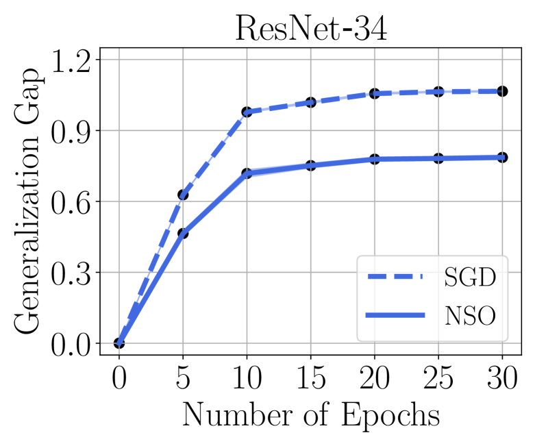
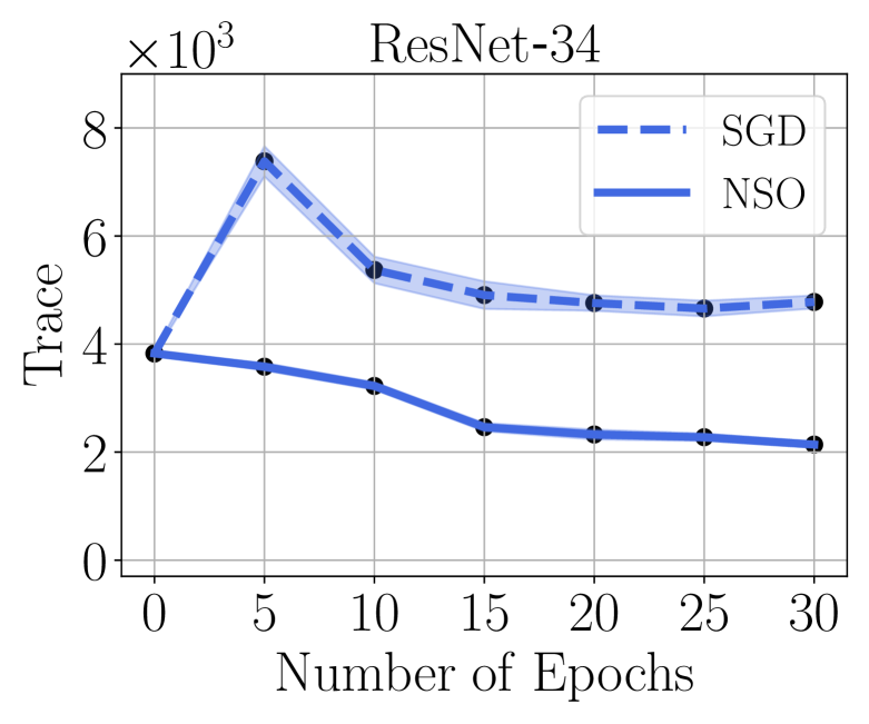
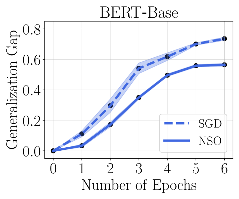
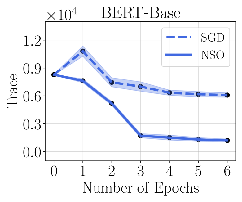
Figure 1: Training curves comparing NSO and SGD; NSO adds a penalty that biases to minimizers with lower Hessian trace compared to SGD and incurs a lower generalization gap.

3 Upper Bound

Our first result gives a fine-grained convergence analysis of the noise stability optimization algorithm. Since finding global minimizers of an arbitrary nonconvex function takes exponential time in the worst case, we focus on finding approximate first-order stationary points in this paper. We state the following assumptions.

Assumption 3.1.

Let $C_{1},C_{2},D$ be fixed, positive constants. First, the initialization $W_{0}\in^{d}$ satisfies $F(W_{0})-\min_{\small W\in^{d}}F(W)\leq D^{2}$. Second, the gradient of $f(W)$ exists and is $C_{1}$-Lipschitz continuous: For any $W_{1}\in^{d}$ and $W_{2}\in^{d}$, the following holds

$$\left\|\nabla f({W_{2}})-\nabla f({W_{1}})\right\|\leq C_{1}\left\|W_{2}-W_{1}\right\|.$$ (5)

A simple corollary of the above is that $\nabla F(W)$ is also Lipschitz-continuous.

Proposition 3.2.

Suppose condition (5) holds. Then, $\nabla F(W)$ is also $C_{1}$-Lipschitz-continuous.

To see this, we apply Eq. (5) inside the expectation of $F(W)$. For any $W_{1},W_{2}\in^{d}$, by definition,

$$\left\|\nabla F(W_{1})-\nabla F(W_{2})\right\| =\left\|\nabla\mathop{\mathbb{E}}_{U\sim\mathcal{P}}\left[f({W_{1}+U})\right]-\nabla\mathop{\mathbb{E}}_{U\sim\mathcal{P}}\left[f({W_{2}+U})\right]\right\|$$

$$=\left\|\mathop{\mathbb{E}}_{U\sim\mathcal{P}}\left[\nabla f({W_{1}+U})-\nabla f({W_{2}+U})\right]\right\|$$

$$\leq\mathop{\mathbb{E}}_{U\sim\mathcal{P}}\left[\left\|\nabla f({W_{1}+U})-\nabla f({W_{2}+U})\right\|\right]\leq C_{1}\left\|W_{1}-W_{2}\right\|.$$

In the event that $f(W)$ is twice-differentiable and the Hessian matrix of $f(W)$ is $C_{2}$-Lipschitz continuous, then the following holds:

$$\left\|\mathbf{H}\big{[}f({W_{2}})\big{]}-\mathbf{H}\big{[}f({W_{1}})\big{]}\right\|_{2}\leq C_{2}\left\|W_{2}-W_{1}\right\|,\text{ for any }W_{1},W_{2}\in^{d}.$$ (6)

For a random variable $U\sim\mathcal{P}$, let the second moment $\mathbb{E}[\|U\|^{2}]$ be denoted as $H(\mathcal{P})$ and the fourth moment $\mathbb{E}[\|U\|^{4}]$ be $G(\mathcal{P})$. Now we can state our first result. There are two cases, depending on whether or not the Hessian exists.

Theorem 3.3.

Suppose Assumptions 2.1 and 3.1 hold. Let $\mathcal{P}$ be a distribution that is symmetric at zero. There exists a fixed learning rate $\eta<C_{1}^{-1}$ such that if we run Algorithm 1 with $\eta_{i}=\eta$ for all $i$, arbitrary number of perturbations $k$, for $T\gtrsim\frac{k}{\sigma^{2}}$ steps, the algorithm returns $W_{t}$ such that

$$\mathop{\mathbb{E}}\left[\left\|\nabla F(W_{t})\right\|^{2}\right]\leq 4D\sqrt{\frac{C_{1}^{3}H(\mathcal{P})+C_{1}\sigma^{2}}{k\cdot T}},$$ (7)

in expectation over the randomness of $t$, perturbations, and gradient queries. Additionally, when $f(\cdot)$ is twice-differentiable and its Hessian is $C_{2}$-Lipschitz-continuous, then the following is also true

$$\mathop{\mathbb{E}}\left[\left\|\nabla F(W_{t})\right\|^{2}\right]\leq 4D\sqrt{\frac{C_{1}C_{2}^{2}G(\mathcal{P})+C_{1}\sigma^{2}}{k\cdot T}}.$$ (8)

The only difference in (7) and (8) is their dependence on $\mathcal{P}$. Let us consider $\mathcal{P}=N(0,\sigma^{2}\operatorname{Id}_{d})$ for example. For small perturbations, the fourth moment $G(\mathcal{P})=(d^{2}+2d)\sigma^{4}$ is smaller than the second moment $H(\mathcal{P})=d\sigma^{2}$. More precisely, when $\sigma^{2}\leq C_{1}^{2}C_{2}^{-2}(d+2)^{-1}$, Eq. (8) gives a tighter bound than (7).

3.1 Proof Overview

Recall that Algorithm 1 involves averaging the gradients at $W+U$ and $W-U$ for $k$ perturbations $U$. This is equivalent to applying SGD to the following symmetrized loss:

$$F(W)=\mathop{\mathbb{E}}_{U\sim\mathcal{P}}\left[\frac{1}{2}\Big{(}f(W+U)+f(W-U)\Big{)}\right].$$ (9)

We provide a motivating example to illustrate the rationale behind the symmetrized gradient.

Example 3.4.

Let $u$ be a Gaussian random variable with mean zero and variance $\sigma^{2}$. Let $f(w)=\frac{1}{4}w^{4}$. Thus, by definition from Eq. 1, $F(w)=\frac{1}{4}\mathbb{E}_{u}[(w+u)^{4}]$. Let us compare the variance of

$$T=\frac{1}{2}(\nabla f(w+u)+\nabla f(w-u))\text{ and }G=\frac{1}{2}(\nabla f(w+u)+\nabla f(w+u^{\prime})),$$

where $u^{\prime}$ is another independent sample from the same distribution as $u$. Notice that both $T$ and $G$ require two gradient queries; Interestingly, $T$ has a lower variance than $G$:

$$\textup{var}[T]=18w^{2}\sigma^{4}<\textup{var}[G]=18w^{2}\sigma^{4}+4.5w^{4}\sigma^{2}+7.5\sigma^{6}.$$ (10)

See Sec. 5 for a comparison between these two gradients in more realistic settings.

Next, we characterize the variance of the stochastic gradient. For $i=0,\dots,T-1$, denote

$$\delta_{i} :=\frac{1}{2k}\sum_{j=1}^{k}\Big{(}\nabla f\big{(}{W_{i}+U_{i}^{(j)}}\big{)}+\nabla f\big{(}{W_{i}-U^{(j)}_{i}}\big{)}\Big{)}-\nabla F(W_{i})$$ (11)

$$\xi_{i} :=\frac{1}{2k}\sum_{j=1}^{k}\Big{(}g_{z_{i}^{(j)}}\big{(}W_{i}+U_{i}^{(j)}\big{)}-\nabla f\big{(}{W_{i}+U_{i}^{(j)}}\big{)}+g_{z_{i}^{(j)}}\big{(}W_{i}-U_{i}^{(j)}\big{)}-\nabla f\big{(}{W_{i}-U_{i}^{(j)}}\big{)}\Big{)}.$$ (12)

It is not hard to see that the mean of $\delta_{i}$ and $\xi_{i}$ are both zero. The former is by the symmetry of $\mathcal{P}$ (cf. Eq. (9)). The latter is because $g_{z}$ is unbiased (cf. Eq. (3)). Next, we give the second moment of $\delta_{i}$ and $\xi_{i}$. The key is that both of their variances scale as $\frac{1}{k}$, where $k$ is the number of noise injections.

Lemma 3.5.

For any $i=1,\dots,T$, suppose  $\nabla f(W)$ is $C_{1}$-Lipschitz, then

$$\mathbb{E}\left[\left\|\xi_{i}\right\|^{2}\right]\leq\frac{\sigma^{2}}{k}~{}~{}and~{}~{}\mathbb{E}\left[\left\|\delta_{i}\right\|^{2}\right]\leq\frac{C_{1}^{2}H(\mathcal{P})}{k}.$$ (13)

Additionally, suppose  $\mathbf{H}[f(W)]$ is $C_{2}$-Lipschitz, then

$$\mathbb{E}\left[\left\|\delta_{i}\right\|^{2}\right]\leq\frac{3C_{2}^{2}G(\mathcal{P})}{8k}.$$ (14)

The proof of Lemma 3.5, based on Proposition 3.2, can be found in App. B.1. These results are needed in the analysis of the gradient dynamic. In particular, the following result is based on results in [44] (cf. App. B.2).

Lemma 3.6.

In the setting of Theorem 3.3, for any $\eta_{0},\cdots,\eta_{T-1}$ less than ${C_{1}}^{-1}$ and a random variable according to a distribution $\Pr[t=j]=\frac{\eta_{j}}{\sum_{i=0}^{T-1}\eta_{i}}$, for any $j=0,\dots,T-1$, the following holds:

$$\mathop{\mathbb{E}}\left[\left\|\nabla F(W_{t})\right\|^{2}\right]\leq\frac{2C_{1}}{\sum_{i=0}^{T-1}\eta_{i}}D^{2}+\frac{C_{1}\sum_{i=0}^{T-1}\eta_{i}^{2}\big{(}\mathop{\mathbb{E}}\left[\left\|\delta_{i}\right\|^{2}\right]+\mathop{\mathbb{E}}\left[\left\|\xi_{i}\right\|^{2}\right]\big{)}}{\sum_{i=0}^{T-1}\eta_{i}}.$$ (15)

Proof of Theorem 3.3    Let the step sizes be equal to a fixed $\eta$ for all epochs. Thus, Eq. (15) becomes

$$\mathop{\mathbb{E}}\left[\left\|\nabla F(W_{t})\right\|^{2}\right]\leq\frac{2}{T\eta}D^{2}+\frac{C_{1}\eta}{T}\sum_{i=0}^{T-1}\Big{(}\mathop{\mathbb{E}}\left[\left\|\delta_{i}\right\|^{2}\right]+\mathop{\mathbb{E}}\left[\left\|\xi_{i}\right\|^{2}\right]\Big{)}.$$ (16)

Minimizing over $\eta$ above leads us to the following upper bound on the right-hand side of (16)

$${2T^{-1}\sqrt{2C_{1}}\cdot D\sqrt{\sum_{i=0}^{T-1}\Big{(}\mathop{\mathbb{E}}\left[\left\|\delta_{i}\right\|^{2}\right]+\mathop{\mathbb{E}}\left[\left\|\xi_{i}\right\|^{2}\right]\Big{)}}}{}.$$

The proof of Eqs. (7) and (8) follows by applying Lemma 3.5 to the above. Recall that the step size $\eta$ must be less than $\eta\leq{C_{1}}^{-1}$. Thus, we must have the following

$$\eta=\frac{D}{\sqrt{\sum_{i=0}^{T-1}\Big{(}\mathop{\mathbb{E}}\left[\left\|\delta_{i}\right\|^{2}\right]+\mathop{\mathbb{E}}\left[\left\|\xi_{i}\right\|^{2}\right]\Big{)}}}\sqrt{\frac{2}{C_{1}}}\leq\frac{1}{C_{1}}\Rightarrow\frac{2C_{1}D^{2}k}{C_{1}^{2}H(\mathcal{P})+\sigma^{2}}\leq T,$$

by applying Eq. (13) to the above. For Eq. (8), the condition is similar and is omitted. In either case, as long as $T\gtrsim\frac{k}{\sigma^{2}}$, then Eqs. (7) and (8) must hold. $\blacksquare$

4 Lower Bound

Next, we complement the upper bound with a matching lower bound. We state a convex example first (which corresponds to Eq. (7)), then a nonconvex example (which corresponds to Eq. (8)). Both apply to SGD, and we will discuss extensions to momentum and adaptive learning rates.

4.1 A Convex Example

We focus on iterative algorithms in the form of update (2) in Algorithm 1. We consider a quadratic function

$$f(W)=\frac{C_{1}}{2}\left\|W\right\|^{2}.$$ (17)

The argument holds for any distribution $\mathcal{P}$ with mean zero. The stochastic objective $F(W)$ is equal to $f(W)+C_{1}\cdot H(\mathcal{P})/2$. The SGD path of Algorithm 1 evolves as follows:

$$W_{t+1} =W_{t}-\eta_{t}\cdot\frac{1}{2k}\sum_{j=1}^{k}\Bigg{(}C_{1}\Big{(}W_{t}+U_{t}^{(j)}\Big{)}+C_{1}\Big{(}W_{t}-U_{t}^{(j)}\Big{)}\Bigg{)}-\eta_{t}\bar{\xi}_{t},$$

$$=\Big{(}1-C_{1}\eta_{t}\Big{)}W_{t}-\eta_{t}\bar{\xi}_{t},$$ (18)

where we denote $\bar{\xi}_{t}$ as the averaged noise $\frac{1}{k}\sum_{j=1}^{k}\xi_{t}^{(j)}$. The key observation is that the gradient noise sequence $\bar{\xi}_{1},\bar{\xi}_{2},\dots,\bar{\xi}_{T}$ forms a martingale sequence:

• For any $i=1,2,\dots,T$, conditioned on the previous random variables $\xi_{i^{\prime}}^{(j)}$ for any $i^{\prime}<i$ and any $j=1,2,\dots,k$, the expectation of $\bar{\xi}_{i}$ is equal to zero.

• The variance of $\bar{\xi}_{i}$ is equal to $\frac{\sigma^{2}}{k}$, since conditional on the previous random variables, the $\xi_{i}^{(j)}$s are all independent from each other.

This martingale property lets us characterize the SGD path of $W_{t}$, as shown in the following result.

Lemma 4.1.

Consider $f$ specified in Eq. (17). For any step sizes $\eta_{0},\dots,\eta_{T-1}$ less than $C_{1}^{-1}$, we have

$$\min_{1\leq t\leq T}\mathop{\mathbb{E}}\left[\left\|\nabla F(W_{t})\right\|^{2}\right]=\min_{1\leq t\leq T}\Big{(}{2C_{1}D^{2}}\prod_{j=0}^{t-1}\big{(}1-C_{1}\eta_{j}\big{)}^{2}+\frac{C_{1}\sigma^{2}}{k}\sum_{i=0}^{t-1}\eta_{i}^{2}\prod_{j=i+1}^{t-1}\big{(}1-C_{1}\eta_{j}\big{)}^{2}\Big{)}.$$ (19)

Proof.

By iterating over Eq. (18), we can get

$$W_{t}=W_{0}\prod_{j=0}^{t-1}\Big{(}1-C_{1}\eta_{j}\Big{)}-\sum_{i=0}^{t-1}\eta_{i}\bar{\xi}_{i}\prod_{j=i+1}^{t-1}\Big{(}1-C_{1}\eta_{j}\Big{)}.$$ (20)

Meanwhile,

$$\nabla F(W_{t})=\nabla f(W_{t})=C_{1}W_{t}\Rightarrow\left\|\nabla F(W_{t})\right\|^{2}=C_{1}^{2}\left\|W_{t}\right\|^{2}.$$

Thus, following Eq. (20), we can get

$$\mathop{\mathbb{E}}\left[\left\|\nabla F(W_{t})\right\|^{2}\right] =C_{1}^{2}\left\|W_{0}\right\|^{2}\prod_{j=0}^{t-1}\Big{(}1-C_{1}\eta_{j}\Big{)}^{2}+C_{1}^{2}\sum_{i=0}^{t-1}\mathop{\mathbb{E}}\left[\left\|\eta_{i}\bar{\xi}_{i}\prod_{j=i+1}^{t-1}\Big{(}1-C_{1}\eta_{j}\Big{)}\right\|^{2}\right]$$ (21)

Above, we use martingale property a), which says the expectation of $\bar{\xi}_{i}$ is equal to zero, for all $i$. In addition, based on property b), the second term in the right of Eq. (21) is equal to

$$C_{1}^{2}\sum_{i=0}^{t-1}\eta_{i}^{2}\left(\prod_{j=i+1}^{t-1}\Big{(}1-C_{1}\eta_{j}\Big{)}^{2}\mathop{\mathbb{E}}\left[\left\|\bar{\xi}_{i}\right\|^{2}\right]\right)=\frac{C_{1}^{2}\sigma^{2}}{k}\sum_{i=0}^{t-1}\eta_{i}^{2}\prod_{j=i+1}^{t-1}\Big{(}1-C_{1}\eta_{j}\Big{)}^{2}.$$

To see this, based on the martingale property of $\bar{\xi}$:

• The cross terms between $\bar{\xi}_{i}$ and $\bar{\xi}_{j}$ for different $i,j$ are equal to zero in expectation:

  $$\mathop{\mathbb{E}}\left[\langle\bar{\xi}_{i},\bar{\xi}_{j}\rangle|\bar{\xi}_{j}\right]=0,\text{ for all }1\leq j<i\leq T.$$

• Additionally, the second moment of $\bar{\xi}_{i}$ is equal to $\frac{\sigma^{2}}{k}$:

  $$\mathop{\mathbb{E}}\left[\left\|\bar{\xi}_{i}\right\|^{2}\right]=\frac{\sigma^{2}}{k},\text{ for any }i=1,\dots,T.$$

Lastly, let $W_{0}$ be a vector such that

$$\left\|W_{0}\right\|=D\sqrt{{2}C_{1}^{-1}}\Rightarrow F({W_{0}})-\min_{W\in^{d}}F(W)\leq D^{2}.$$

Inserting the above value of $W_{0}$ to Eq. (21) leads to

$$\mathop{\mathbb{E}}\left[\left\|\nabla F(W_{t})\right\|^{2}\right]=2C_{1}D^{2}\prod_{j=0}^{t-1}\Big{(}1-C_{1}\eta_{j}\Big{)}^{2}+\frac{C_{1}^{2}\sigma^{2}}{k}\sum_{i=0}^{t-1}\eta_{i}^{2}\prod_{j=i+1}^{t-1}\Big{(}1-C_{1}\eta_{j}\Big{)}^{2}$$ (22)

By taking the minimum over $t=1,\dots,T$, we conclude that Eq. (19) holds. ∎

This result applies to arbitrary learning rates. Next, we show a simpler statement for a slightly different quadratic function

$$f(W)=\frac{1}{2\kappa}\left\|W\right\|^{2},\text{ where }\kappa=\max\{C_{1}^{-1},2\sum_{i=0}^{T-1}\eta_{i}\},$$ (23)

which will be easier to work with for small learning rates, as we shall see next.

Lemma 4.2.

Consider $f$ given in Eq. (23) above. For any step sizes $\eta_{0},\dots,\eta_{T-1}$ less than $C_{1}^{-1}$, the following holds for the stochastic objective $F$:

$$\min_{1\leq t\leq T}\mathop{\mathbb{E}}\left[\left\|\nabla F(W_{t})\right\|^{2}\right]\geq\frac{D^{2}}{2\max\{C_{1}^{-1},2\sum_{i=0}^{T-1}\eta_{i}\}}.$$ (24)

The proof of Eq. 24 is similar to Lemma 4.1; See details in App. B.3. Now we are ready to state the main result of this section.

Theorem 4.3.

There exists convex quadratic functions $f$ such that for any gradient oracle satisfying Assumption 2.1 and any distribution $\mathcal{P}$ with mean zero, if $\eta_{i}=\eta<C_{1}^{-1}$ for any $i=1,\dots,T$, or if $\sum_{i=0}^{T-1}\eta_{i}\lesssim\sqrt{T}$, then the following must hold:

$$\min_{1\leq t\leq T}\mathop{\mathbb{E}}\left[\left\|\nabla F(W_{t})\right\|^{2}\right]\geq D\sqrt{\frac{C_{1}\sigma^{2}}{32k\cdot T}}.$$ (25)

The result of Eq. (25) matches the upper bound for twice-differentiable functions in Eq. (8). More precisely, for small perturbations when the moments $H(\mathcal{P})$ and $G(\mathcal{P})$ are constants, e.g., when $\mathcal{P}=N(0,d^{-1}\operatorname{Id}_{d})$, the lower bound matches the upper bound up to constants.

4.1.1 Proof of Convex Lower Bound

By Lemma 4.2, there exists a function such that the left-hand side of Eq. (25) is at least

$$\frac{D^{2}}{2\max\{C_{1}^{-1},2\sum_{i=0}^{T-1}\eta_{i}\}}\geq\frac{C_{1}D^{2}}{2\max\{1,2x^{-1}\sqrt{T}\}}=\frac{D^{2}x}{4\sqrt{T}},$$ (26)

which holds if $\sum_{i=0}^{T-1}\eta_{i}\leq\sqrt{T}x^{-1}$ for any fixed $x>0$.

On the other hand, if $\sum_{i=0}^{T-1}\eta_{i}\geq x^{-1}\sqrt{T}$ and $\eta_{i}=\eta$ for a fixed $\eta$, then $\eta>x^{-1}/\sqrt{T}$. By setting $\eta_{i}=\eta$ for all $i$ in Lemma 4.1, the left-hand side of Eq. (25) is equal to

$$\min_{1\leq t\leq T}\left(2C_{1}D^{2}(1-C_{1}\eta)^{2t}+\frac{C_{1}^{2}\sigma^{2}}{k}\sum_{k=0}^{t-1}\eta^{2}(1-C_{1}\eta)^{2(t-k-1)}\right).$$

Recall that $\eta<C_{1}^{-1}$. Thus, $\rho=C_{1}\eta$ must be strictly less than one. With some calculation, we can simplify the above to

$$\min_{1\leq t\leq T}\left(2C_{1}D^{2}(1-\rho)^{2t}+\frac{\sigma^{2}\rho^{2}}{k}\frac{1-(1-\rho)^{2t}}{1-(1-\rho)^{2}}\right)$$

$$= \min_{1\leq t\leq T}\left(\frac{\sigma^{2}\rho}{k(2-\rho)}+(1-\rho)^{2t}\Big{(}2C_{1}D^{2}-\frac{\sigma^{2}\rho}{k(2-\rho)}\Big{)}\right).$$ (27)

If $2C_{1}D^{2}<\frac{\sigma^{2}\rho}{k(2-\rho)}$, the above is the smallest when $t=1$. In this case, Eq. (27) is equal to

$$2C_{1}D^{2}(1-\rho)^{2}+\frac{\sigma^{2}\rho^{2}}{k}\geq\frac{1}{\frac{1}{2C_{1}D^{2}}+\frac{k}{\sigma^{2}}}=O(1).$$

If $2C_{1}D^{2}\geq\frac{\sigma^{2}\rho}{k(2-\rho)}$, the above is the smallest when $t=T$. In this case, Eq. (27) is at least

$$\frac{\sigma^{2}\rho}{k(2-\rho)}\geq\frac{\sigma^{2}\rho}{2k}\geq\frac{\sigma^{2}C_{1}x^{-1}}{2k}\cdot\frac{1}{\sqrt{T}}.$$ (28)

To conclude the proof, we set $x$ so that the right-hand side of (26) and (28) match each other. This leads to

$$x=\sqrt{\frac{2\sigma^{2}C_{1}}{kD^{2}}}.$$

Thus, by combining the conclusions from both (26) and (28) with this value of $x$, we finally conclude that if $\sum_{i=0}^{T-1}\eta_{i}\leq\sqrt{T}x^{-1}$, or for all $i=0,\dots,T-1$, $\eta_{i}=\eta<C_{1}^{-1}$, then in both cases, there exists a function $f$ such that Eq. (25) holds. This completes the proof of Theorem 4.3. $\blacksquare$

Our construction is inspired by the SGD lower bound of [59] for convex functions. Our analysis above gives a more fine-grained characterization of the SGD noise. Moreover, the analysis applies to any gradient oracle (with mean zero and bounded variance), which may be of independent interest.

4.2 A Nonconvex Example

Next, we construct a nonconvex function. Let $e_{t}$ be the basis vector for the $t$-th dimension, for $t=0,1,\dots,T-1$. We consider a chain-like function:

$$f(W)=\frac{1}{2G}\langle W,e_{0}\rangle^{2}+\sum_{i=0}^{T-1}h_{i}(\langle W,e_{i+1}\rangle),$$ (29)

where $h_{i}$ a quadratic function parametrized by $\alpha_{i}$, defined as follow:

$$h_{i}(x)=\left\{\begin{array}[]{ll}\frac{1}{4}C_{1}\alpha_{i}^{2}&|x|\leq\alpha_{i},\\ -\frac{1}{2}C_{1}\big{(}|x|-\alpha_{i}\big{)}^{2}+\frac{1}{4}C_{1}\alpha_{i}^{2}&\alpha_{i}\leq|x|\leq\frac{3}{2}\alpha_{i},\\ \frac{1}{2}C_{1}\big{(}|x|-2\alpha_{i}\big{)}^{2}&\frac{3}{2}\alpha_{i}\leq|x|\leq 2\alpha_{i},\\ 0&2\alpha_{i}\leq|x|.\end{array}\right.$$

See Figure 2 for several examples of this function.

One can verify that $\nabla h_{i}$ is $C_{1}$-Lipschitz but is not differentiable. Additionally, $\nabla f$ is $C_{1}$-Lipschitz when $G\leq C_{1}^{-1}$ (cf. Eq. (29)). As for the other parts of the construction:

• Let $W_{0}$ satisfy that $\langle W_{0},e_{i}\rangle=0$ for any $i\geq 1$ while $\langle W_{0},e_{0}\rangle\neq 0$.

• Let $\mathcal{P}$ satisfy that the $i$-th coordinate is at most $2^{-1}\alpha_{i-1}$, for $i=1,\dots,T$.

• Let the gradient oracle be chosen such that the $i$-th step’s gradient noise $\xi_{i}=\langle\xi_{i},e_{i+1}\rangle e_{i+1}$. This implies only coordinate $i+1$ is updated in step $i$, as long as $\langle\xi_{i},e_{i+1}\rangle\leq 2^{-1}\alpha_{i}$.

Based on this construction, in step $i$, the gradient noise $\xi_{i}$ plus the perturbation noise is less than $\alpha_{i}$ at coordinate $i+1$. Thus, we have that $h_{i}^{\prime}(\langle W_{t},e_{i+1}\rangle)=0$. This implies $\nabla f(W_{i})$ is equal to $G^{-1}\langle W_{i},e_{0}\rangle$. Roughly speaking, the above construction will go through provided the learning rate $\eta_{i}$ is smaller than $\alpha_{i}$. Recall from Assumption (3.1) that $F(W_{0})\leq D^{2}$, which is the same as $\sum_{i=0}^{T-1}\alpha_{t}^{2}\leq D^{2}$. With some calculation, the learning rates must satisfy $\sum_{i=0}^{T-1}\eta_{i}\lesssim\sqrt{T}$. This ensures the iterates will be trapped close to $W_{0}$ even after $T$ steps; Thus, the gradient of every iterate must be “large”. The details are stated in Lemma B.3, App. B.4.

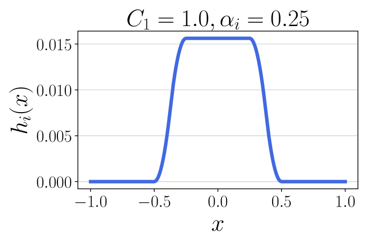
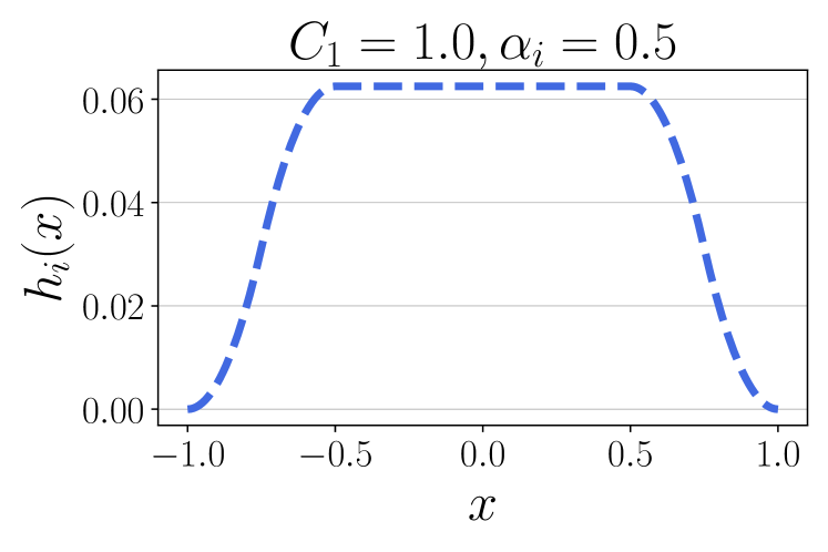
Figure 2: Examples of piecewise quadratic functions $h_{i}$ with Lipschitzness $C_{1}$ and parameter $\alpha_{i}$.

When the learning rate is fixed at $\eta\gtrsim T^{-1/2}$, we construct a chain-like function as above but use a different piece-wise quadratic function with a fixed $\alpha$ (cf. Lemma B.4, App. B.4). The gradient noise grows by $1-\eta/C_{1}$ up to $T$ steps at each step. We then carefully set $\alpha$ to lower bound the norm of the gradient. Based on these two results, we state the lower bound for a nonconvex example.

Theorem 4.4.

Suppose the learning rates $\eta_{0},\dots,\eta_{T-1}$ are at most $C_{1}^{-1}$ and satisfy $\sum_{i=0}^{T-1}\eta_{i}\lesssim\sqrt{kT}$ or $\eta_{i}=\eta<C_{1}^{-1}$ for any epoch $i$. There exists a nonconvex, differentiable, but not twice-differentiable function $f:^{d}\rightarrow$ with dimension $d\geq T$ satisfying Assumption 3.1, a gradient oracle satisfying Assumption 2.1, and perturbation distribution $\mathcal{P}$ such that the following is true

$$\min_{1\leq t\leq T}\mathop{\mathbb{E}}\left[\left\|\nabla F(W_{t})\right\|^{2}\right]\geq D\sqrt{\frac{C_{1}\sigma^{2}}{32k\cdot T}}.$$ (30)

One can see that the rate in Eq. (30) again matches our upper bound for the case of differentiable functions in Eq. (7), when $H(\mathcal{P})$ is a constant (e.g. when $\mathcal{P}=N(0,d^{-1}\operatorname{Id}_{d})$.

4.3 Extensions

The lower bound regarding convex functions can be naturally extended to momentum SGD:

$$V_{t+1}=\mu V_{t}-\eta_{t}G_{t},\text{ and }M_{t+1}=M_{t}+V_{t+1},$$ (31)

where $G_{t}$ refers to the stochastic gradient in Eq. (2). This can be seen by generalizing the argument of Lemma 4.1 to weighted combinations of iterates. We state the following corollary, leaving its proof to Appendix B.5.

Corollary 4.5.

There exists a convex quadratic function satisfying Assumption 3.1 with Lipschitz Hessians such that for $M_{1},\dots,M_{T}$ following momentum SGD, the following must be true:

$$\min_{1\leq t\leq T}\mathop{\mathbb{E}}\left[\left\|\nabla F(M_{t})\right\|^{2}\right]\gtrsim D\sqrt{\frac{C_{1}\sigma^{2}}{k\cdot T}}.$$ (32)

Next, we discuss extensions to SGD with adaptive learning rates. Again, notice that the proof of Lemma 4.2 holds for any arbitrary learning rates. Furthermore, the proof of Theorem 4.4 also applies to any learning rates under certain bounded conditions. It is conceivable that similar results can be derived for SGD with adaptive step sizes under similar bounded conditions when $\eta_{i}$ is a function of previous weights and step size.

The construction for the nonconvex case can also be extended to SGD with adaptive learning rates such as AdaGrad. To see this, notice that the proof of Lemma B.3 does not use any specific properties of the learning rates. In fact, we can set the width of each $h_{t}$ function, $\alpha_{t}$, in proportion to the learning rate $\eta_{t}$, for an arbitrary $t$. Thus, even if the algorithm uses an adaptive learning rate schedule such as AdaGrad, the construction can still go through.

5 Numerical Results

This section conducts experiments to evaluate the empirical benefits of our algorithm. We evaluate Algorithm 1 by fine-tuning pretrained neural nets on image classification datasets, including online medical image classification datasets containing eye fundus images for diabetic retinopathy classification, and several natural image classification datasets, including Aircrafts, Birds, and Indoor. We compare our algorithm with stochastic gradient descent (SGD) and sharpness-aware minimization (SAM). We sample perturbations from isotropic Gaussian distribution $N(0,\sigma^{2}\operatorname{Id}_{d})$ and tune $\sigma$ among $0.008,0.01$, and $0.012$. To evaluate the trace and eigenvalues of the loss Hessian matrix, we use Hessian vector products. Other details about the implementation are provided in App. A.

First, we justify both rationales of our design in Sec. 2. The first compares NSO with weight-perturbed SGD using two independently sampled random gradient estimates (cf. Example 3.4). We validate that NSO can reduce the largest eigenvalue ($\lambda_{1}$) and the Hessian trace by 8.6% more. The second studies the effect of increasing $k$, as using larger $k$ in NSO would lead to a better estimation of the gradient. We vary $k=1,2,3$ on both datasets. The results are shown in Table 1 below.

Table 1: We describe several ablation studies to understand the relationship between different algorithms. (1) With the same number of gradient queries, NSO can converge to minimizers with lower $\lambda_{1}$ than weight-perturbed SGD, and achieve better test accuracy. (2) As we add more perturbations, the largest eigenvalue of Hessian decreases further, and similar results also apply to the Hessian trace.

Dataset: Aircrafts	Test accuracy ($\uparrow$)	$\lambda_{1}[\mathbf{H}]$ ($\downarrow$)	Dataset: Indoor	Test accuracy ($\uparrow$)	$\lambda_{1}[\mathbf{H}]$ ($\downarrow$)
WP-SGD ($k=2$)	60.63$\pm$0.38	675$\pm$58	WP-SGD ($k=2$)	76.49$\pm$0.40	748$\pm$53
NSO ($k=1$)	62.31$\pm$0.36	612$\pm$44	NSO ($k=1$)	77.39$\pm$0.55	688$\pm$58
WP-SGD ($k=4$)	60.40$\pm$0.39	597$\pm$47	WP-SGD ($k=4$)	77.11$\pm$0.31	688$\pm$44
NSO ($k=2$)	63.46$\pm$0.43	567$\pm$63	NSO ($k=2$)	77.44$\pm$0.30	652$\pm$56
WP-SGD ($k=6$)	60.79$\pm$0.69	685$\pm$63	WP-SGD ($k=6$)	77.34$\pm$0.44	658$\pm$37
NSO ($k=3$)	63.64$\pm$0.68	550$\pm$39	NSO ($k=3$)	77.94$\pm$0.64	630$\pm$74

Next, we report results comparing both the Hessian trace and $\lambda_{1}$ of iterates at the final epoch. Curiously, NSO achieves notably smaller $\lambda_{1}$ and Hessian trace. Figure 3 visualizes this comparison. Due to space limit, the detailed results (including a comparison of empirical test performance) are reported in Table 3, App. A.

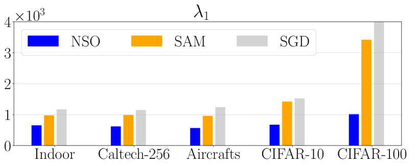
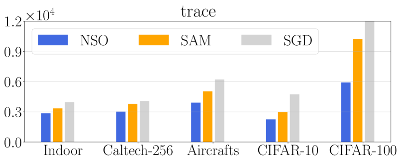
Figure 3: Comparing the loss Hessian’s largest eigenvalue and trace between NSO, SAM, and SGD, conducted on ResNet-34, averaged over three random seeds. Interestingly, NSO finds minimizers with lower Hessian trace than SAM. We hypothesize this is because the algorithm minimizes an objective that involves an explicit penalty on the Hessian trace. Formally explaining this behavior is an interesting question for future work.

Appendix A Experiment Details

We describe setups and results left from the main text. We consider two types of image classification datasets. First, we use two medical image datasets related to diabetic retinopathy classification using eye fundus images. Each dataset contains the interior surface images of a single eye and labels regarding the severity of diabetic retinopathy of the eye. The two datasets are available in the following sources: Retina I (Messidor) and Retina II (APTOS) . Second, we consider fine-grained image classification datasets, including Aircrafts , Birds, and Indoor. Besides, we use the following datasets to illustrate the consistent performance of our algorithm, including Flowers, Cars, Caltech-256, CIFAR-10, and CIFAR-100. We report the dataset statistics in Table 2.

Table 2: Basic statistics for image classification tasks.

	Retina I	Retina II	Aircrafts	Birds	Indoor	Flowers	Cars	Caltech-256	CIFAR-10	CIFAR-100
Training	1,396	2,930	3,334	5,395	4,824	1,020	7,330	7,680	45,000	45,000
Validation	248	732	3,333	599	536	1,020	814	5,120	5,000	5,000
Test	250	733	3,333	574	1,340	6,149	8,441	5,120	10,000	10,000
Classes	5	5	100	200	67	102	196	256	10	100

Table 3: Top panel: Largest eigenvalue of neural net loss Hessian matrix. Middle panel: Hessian trace. Lower panel: Test accuracy. All results are averaged over three random seeds.

Dataset	Retina I	Retina II	Aircrafts	Birds	Indoor
SGD	8,996$\pm$92	2,413$\pm$32	1,239$\pm$43	1,286$\pm$76	1,169$\pm$66
LS	4,911$\pm$73	1,494$\pm$99	1,339$\pm$84	992$\pm$55	876$\pm$81
SAM	4,246$\pm$55	1,341$\pm$26	958$\pm$60	1,061$\pm$49	975$\pm$56
ASAM	4,267$\pm$58	1,629$\pm$41	641$\pm$89	1,089$\pm$56	722$\pm$56
NSO (Alg. 1)	3,916$\pm$47	1,095$\pm$49	612$\pm$44	1,045$\pm$68	688$\pm$58
SGD	30,433$\pm$217	6,921$\pm$54	6,218$\pm$63	4,252$\pm$93	4,078$\pm$78
LS	19,219$\pm$119	4,559$\pm$49	6,332$\pm$76	4,585$\pm$79	4,196$\pm$36
SAM	16,411$\pm$161	3,702$\pm$94	5,034$\pm$59	3,515$\pm$48	3,789$\pm$49
ASAM	14,745$\pm$131	4,174$\pm$52	5,191$\pm$32	3,799$\pm$44	3,124$\pm$73
NSO (Alg. 1)	11,554$\pm$77	3,519$\pm$57	4,193$\pm$46	3,067$\pm$65	2,991$\pm$32
SGD	61.69$\pm$0.89	83.70$\pm$0.53	59.76$\pm$0.71	73.34$\pm$0.11	75.95$\pm$0.46
LS	63.56$\pm$0.72	83.65$\pm$0.68	58.47$\pm$0.29	74.38$\pm$0.33	75.87$\pm$0.35
SAM	64.39$\pm$0.66	84.65$\pm$0.78	61.54$\pm$0.82	73.65$\pm$0.65	76.57$\pm$0.56
ASAM	64.79$\pm$0.37	84.88$\pm$0.38	62.02$\pm$0.61	74.72$\pm$0.58	76.72$\pm$0.31
NSO (Alg. 1)	66.57$\pm$0.75	85.24$\pm$0.45	62.31$\pm$0.36	75.35$\pm$0.53	77.39$\pm$0.55

Results on CIFAR. We report fine-tuning results of ResNet-34 on CAFAR-10 and CIFAR-100. Our algorithm achieves 18% and 26% smaller the Hessian eigenvalues and traces, respectively. The results are shown in Table 4.

Table 4: Comparisons on CIFAR datasets. Left: Largest eigenvalue of the loss Hessian matrix. Middle: Hessian trace. Right: Test accuracy. All results are averaged over 3 random seeds.

	Largest Eigenvalue		Trace		Test Accuracy
	CIFAR-10	CIFAR-100	CIFAR-10	CIFAR-100	CIFAR-10	CIFAR-100
Vanilla SGD	1,522 $\pm$ 45	4,870 $\pm$ 88	4,738 $\pm$ 73	14,372 $\pm$ 346	95.48$\pm$0.10	82.25$\pm$0.16
Label smoothing	1,416 $\pm$ 45	3,459 $\pm$ 95	2,903 $\pm$ 92	11,295 $\pm$ 384	96.68$\pm$0.10	83.75$\pm$0.19
SAM	1,372 $\pm$ 49	3,419 $\pm$ 75	2,847 $\pm$ 78	10,230 $\pm$ 385	96.64$\pm$0.47	83.48$\pm$0.16
ASAM	1,425 $\pm$ 67	2,599 $\pm$ 79	2,830 $\pm$ 57	10,478 $\pm$ 263	96.73$\pm$0.16	83.84$\pm$0.12
NSO (Alg. 1)	1,136 $\pm$ 58	2,184 $\pm$ 59	2,061 $\pm$ 70	5,829 $\pm$ 211	97.10$\pm$0.28	84.29$\pm$0.27

Comparing noise stability to Hessian trace. In Table 5, we conduct experiments on a two-layer MLP with MNIST, a 12-layer BERT model on the MRPC dataset from the GLUE benchmark, and a two-layer GCN on the COLLAB dataset from TUDataset. For model architectures, we set both MLP and GCN with a hidden dimension of 128 and initialize them randomly. We initialize the BERT model from pretrained BERT-Base-Uncased. For the training process, we train each model on the provided training set until the training loss is close to zero. Specifically, we train the MLP, BERT, and GCN models for 30, 10, and 100 epochs, respectively.

We use the model of the last epoch to evaluate the noise stability and Hessian traces on the training dataset. For noise stability, we first perturb the model weights by injecting isotropic Gaussian noise into the model weights. We then compute the average loss of the perturbed weights over 100 perturbations minus the loss of the unperturbed weights. For the Hessian trace, we evaluate the average loss of Hessian trace over the training dataset.

We observe that the range of noise variance $\sigma^{2}$, where the Hessian term approximates the noise stability, differs across various networks due to the different weight scales of each network. We select the range so that the noise stability values remain comparable to the actual loss, beyond which the perturbed loss will increase dramatically.

Table 5: We sample 100 perturbations and compute the averaged perturbed loss values. We measure the Hessian trace using PyHessian implementation of Hutchinson’s method which does not require computing the entire Hessian matrix. The reported values are rescaled by $10^{2}$.

MNIST, MLP			MRPC, BERT-Base-Uncased			COLLAB, GCN
$\sigma$	$\mathcal{I}(W)$	$\frac{\sigma^{2}}{2}\operatorname{Tr}[\mathbf{H}]$	$\sigma$	$\mathcal{I}(W)$	$\frac{\sigma^{2}}{2}\operatorname{Tr}[\mathbf{H}]$	$\sigma$	$\mathcal{I}(W)$	$\frac{\sigma^{2}}{2}\operatorname{Tr}[\mathbf{H}]$
0.020	1.22 $\pm$ 0.27	0.96	0.0070	0.83 $\pm$ 0.31	0.95	0.040	2.97 $\pm$ 0.97	2.78
0.021	1.24 $\pm$ 0.26	1.06	0.0071	0.88 $\pm$ 0.31	0.98	0.041	2.66 $\pm$ 1.41	2.92
0.022	1.37 $\pm$ 0.42	1.17	0.0072	0.93 $\pm$ 0.32	1.01	0.042	3.63 $\pm$ 0.86	3.06
0.023	1.42 $\pm$ 0.49	1.28	0.0073	0.98 $\pm$ 0.34	1.03	0.043	2.43 $\pm$ 1.09	3.21
0.024	1.52 $\pm$ 0.46	1.39	0.0074	1.04 $\pm$ 0.35	1.06	0.044	2.87 $\pm$ 1.11	3.36
0.025	1.75 $\pm$ 0.47	1.51	0.0075	1.10 $\pm$ 0.36	1.09	0.045	2.98 $\pm$ 0.92	3.51
0.026	1.82 $\pm$ 0.38	1.63	0.0076	1.17 $\pm$ 0.38	1.12	0.046	4.14 $\pm$ 1.05	3.67
0.027	2.09 $\pm$ 0.35	1.76	0.0077	1.24 $\pm$ 0.40	1.15	0.047	3.13 $\pm$ 1.09	3.83
0.028	2.15 $\pm$ 0.49	1.89	0.0078	1.31 $\pm$ 0.42	1.18	0.048	4.55 $\pm$ 0.89	4.00
0.029	2.44 $\pm$ 0.75	2.03	0.0079	1.39 $\pm$ 0.44	1.21	0.049	4.49 $\pm$ 1.60	4.17
0.030	2.58 $\pm$ 0.59	2.18	0.0080	1.47 $\pm$ 0.47	1.24	0.050	4.82 $\pm$ 1.00	4.34
Relative RSS	2.74%			1.03%			2.16%

Appendix B Proofs for Technical Lemmas

B.1 Proof of Lemma 3.5

The smoothness condition in Assumption 3.1 is equivalent to the following domination inequality:

$${\left|{f({W_{2}})-f({W_{1}})-\langle\nabla f({W_{1}}),W_{2}-W_{1}\rangle}\right|} \leq\frac{C_{1}}{2}\left\|W_{2}-W_{1}\right\|^{2}.$$ (33)

See, e.g., [62, Chapter 5 ]. We state a similar result on the Hessian as follows.

Proposition B.1.

Suppose $f(W)$ is twice-differentiable and the Hessian of $f(W)$ is $C_{2}$-Lipschitz. Then, for any $W_{1}\in^{d}$ and $W_{2}\in^{d}$, the following holds:

$$\left\|\nabla f({W_{2}})-\nabla f({W_{1}})-\mathbf{H}\big{[}f({W_{1}})\big{]}(W_{2}-W_{1})\right\| \leq\frac{C_{2}}{2}\left\|W_{2}-W_{1}\right\|^{2}.$$ (34)

Proof.

We apply a line integral along $W_{2}-W_{1}$ below:

$$\left\|\nabla f({W_{2}})-\nabla f({W_{1}})-\mathbf{H}\big{[}f({W_{1}})\big{]}(W_{2}-W_{1})\right\|$$

$$= \left\|\int_{0}^{1}\mathbf{H}\big{[}f({W_{1}+\tau(W_{2}-W_{1})})\big{]}d\tau(W_{2}-W_{1})-\mathbf{H}\big{[}f({W_{1}})\big{]}(W_{2}-W_{1})\right\|$$

$$= \left\|\int_{0}^{1}\Big{(}\mathbf{H}\big{[}f({W_{1}+\tau(W_{2}-W_{1})})\big{]}-\mathbf{H}\big{[}f({W_{1}})\big{]}\Big{)}(W_{2}-W_{1})d\tau\right\|$$

$$\leq \int_{0}^{1}C_{2}\tau\left\|W_{2}-W_{1}\right\|^{2}d\tau=\frac{C_{2}}{2}\left\|W_{2}-W_{1}\right\|^{2}.$$

∎

Based on the above result, we provide proofs for the variance of $\delta_{i}$ and $\xi_{i}$ for any $i=0,1,\dots,T-1$.

Proof of Lemma 3.5    First, we can see that

$$\mathop{\mathbb{E}}_{U_{i}^{1},\dots,U_{i}^{k}}\left[\left\|\delta_{i}\right\|^{2}\right] =\mathop{\mathbb{E}}_{U_{i}^{1},\dots,U_{i}^{k}}\left[\left\|\frac{1}{2k}\sum_{j=1}^{k}\Big{(}\nabla f({W_{i}+U_{i}^{j}})+\nabla f({W_{i}-U^{j}_{i}})-2\nabla F(W_{i})\Big{)}\right\|^{2}\right]$$

$$=\frac{1}{k^{2}}\sum_{j=1}^{k}\mathop{\mathbb{E}}_{U_{i}^{j}}\left[\left\|\frac{1}{2}\Big{(}\nabla f({W_{i}+U_{i}^{j}})+\nabla f({W_{i}-U^{j}_{i}})-2\nabla F(W_{i})\Big{)}\right\|^{2}\right] U_{i}^{j_{1}}\perp U_{i}^{j_{2}} j_{1}\neq j_{2}$$ ( when )

$$=\frac{1}{k}\mathop{\mathbb{E}}_{U_{i}^{1}}\left[\left\|\frac{1}{2}\Big{(}\nabla f({W_{i}+U_{i}^{1}})+\nabla f({W_{i}-U_{i}^{1}})\Big{)}-\nabla F(W_{i})\right\|^{2}\right] U_{i}^{1},\dots,U_{i}^{k}$$ ( are identical)

In the second step, we use the fact that for two independent random variables $U,V$, and any continuous functions $h(U),g(V)$, $h(U)$ and $g(V)$ are still independent (recall that $f$ is continuous since it is twice-differentiable). We include a short proof of this fact for completeness. If $U$ and $V$ are independent, we have

$$\Pr[U\in A,V\in B]=\Pr[U\in A]\cdot\Pr[V\in B],\forall A,B\in\text{Borel}().$$

Thus, if $h$ and $g$ are continuous functions, we obtain

$$\Pr[h(U)\in A,g(V)\in B]$$

$$= \Pr[U\in h^{-1}(A),V\in g^{-1}(B)]$$

$$= \Pr[U\in h^{-1}(A)]\cdot\Pr[V\in g^{-1}(B)]=\Pr[h(U)\in A]\cdot\Pr[g(V)\in B].$$

Thus, we have shown that

$$\mathop{\mathbb{E}}\left[\left\|\delta_{i}\right\|^{2}\right]=\frac{1}{k}\mathop{\mathbb{E}}_{U\sim\mathcal{P}}\left[\left\|\frac{1}{2}\Big{(}\nabla f(W_{i}+U)+f(W_{i}-U)\Big{)}-\nabla F(W_{i})\right\|^{2}\right].$$ (35)

Next, we deal with the variance of the two-point stochastic gradient, depending on whether $f$ has Lipschitz-Hessian or not. If $f$ has $C_{1}$-Lipschitz gradient, we will show that

$$\mathop{\mathbb{E}}_{U}\left[\left\|\frac{1}{2}\Big{(}\nabla f(W+U)+\nabla f(W-U)\Big{)}-\nabla F(W)\right\|^{2}\right]\leq{2C_{1}^{2}H(\mathcal{P})}.$$ (36)

By equation (33) from Proposition B.1, the left-hand side of equation (36) is equal to

$$\mathop{\mathbb{E}}_{U}\left[\left\|\frac{1}{2}\Big{(}\nabla f(W+U)-\nabla F(W)\Big{)}+\frac{1}{2}\Big{(}\nabla f(W-U)-\nabla F(W)\Big{)}\right\|^{2}\right]$$

$$\leq \mathop{\mathbb{E}}_{U}\left[\frac{1}{2}\left\|\nabla f(W+U)-\nabla F(W)\right\|^{2}+\frac{1}{2}\left\|\nabla f(W-U)-\nabla F(W)\right\|^{2}\right]$$ (by Cauchy-Schwartz inequality)

$$= \frac{1}{2}\mathop{\mathbb{E}}_{U}\left[\left\|\nabla f(W+U)-\nabla F(W)\right\|^{2}\right] \mathcal{P}$$ (by symmetry of since it has mean zero)

$$= \frac{1}{2}\mathop{\mathbb{E}}_{U}\left[\left\|\mathop{\mathbb{E}}_{U^{\prime}\sim\mathcal{P}}\left[\nabla f(W+U)-\nabla f(W+U^{\prime})\right]\right\|^{2}\right]\leq\frac{1}{2}\mathop{\mathbb{E}}_{U}\left[\mathop{\mathbb{E}}_{U^{\prime}\sim\mathcal{P}}\left[\left\|\nabla f(W+U)-\nabla f(W+U^{\prime})\right\|^{2}\right]\right]$$

$$\leq \frac{1}{2}\mathop{\mathbb{E}}_{U,U^{\prime}}\left[C_{1}^{2}\left\|U-U^{\prime}\right\|^{2}\right]=\frac{1}{2}C_{1}^{2}\mathop{\mathbb{E}}_{U,U^{\prime}}\left[\left\|U\right\|^{2}+\left\|U^{\prime}\right\|^{2}\right]=C_{1}^{2}H(\mathcal{P})$$ (by equation (33))

If, in addition, the Hessian of $f$ is $C_{2}$-Lipschitz, we show that

$$\mathop{\mathbb{E}}_{U}\left[\left\|\frac{1}{2}\Big{(}\nabla f(W+U)+\nabla f(W-U)\Big{)}-\nabla F(W)\right\|^{2}\right]\leq\frac{3}{8}C_{2}^{2}G(\mathcal{P}){}.$$ (37)

By equation (34) from Proposition B.1, we know that

$$\left\|\nabla f({W+U})-\nabla f({W})-\mathbf{H}\big{[}f({W})\big{]}U\right\|\leq\frac{C_{2}}{2}\left\|U\right\|^{2},\text{ and }$$ (38)

$$\left\|\nabla f({W-U})-\nabla f({W})+\mathbf{H}\big{[}f({W})\big{]}U\right\|\leq\frac{C_{2}}{2}\left\|U\right\|^{2}.$$ (39)

Next,

$$\mathop{\mathbb{E}}_{U}\left[\left\|\nabla F(W)-\nabla f({W})\right\|^{2}\right]= \left\|\nabla F(W)-\nabla f({W})\right\|^{2}$$ (40)

$$= \left\|\mathop{\mathbb{E}}_{U}\left[\nabla f({W+U})-\nabla f({W})-\mathbf{H}\big{[}f({W})\big{]}U\right]\right\|^{2} \mathop{\mathbb{E}}_{U}\left[U\right]=0$$ (since )

$$\leq \mathop{\mathbb{E}}_{U}\left[\left\|\nabla f({W+U})-\nabla f({W})-\mathbf{H}\big{[}f({W})\big{]}U\right\|^{2}\right]$$ (by Cauchy-Schwartz ineq.)

$$\leq \mathop{\mathbb{E}}_{U}\left[\Big{(}\frac{C_{2}}{2}\left\|U\right\|^{2}\Big{)}^{2}\right],$$ (41)

where the last step uses equation (39). Hence, using triangle inequality, the left-hand side of equation (37) is equal to

$$\frac{1}{k}\mathop{\mathbb{E}}_{U}\left[\left\|\frac{1}{2}\nabla f({W+U})-\frac{1}{2}\nabla F(W)+\frac{1}{2}\nabla f({W-U})-\frac{1}{2}\nabla f({W})+\nabla f({W})-\nabla F(W)\right\|^{2}\right]$$

$$\leq \frac{1}{k}\Bigg{(}\mathop{\mathbb{E}}_{U}\left[\Big{(}\frac{C_{2}}{4}\left\|U\right\|^{2}\Big{)}^{2}+\Big{(}\frac{C_{2}}{4}\left\|U\right\|^{2}\Big{)}^{2}+\Big{(}\frac{C_{2}}{2}\left\|U\right\|^{2}\Big{)}^{2}\right]\Bigg{)}$$ (by combining equations (38), (39), and (41))

$$= \frac{3C_{2}^{2}}{8k}\cdot\mathop{\mathbb{E}}_{U}\left[\left\|U\right\|^{4}\right]=\frac{3C_{2}^{2}}{8k}G(\mathcal{P}).$$

Therefore, we have proved equation (37).

As for the variance of $\xi_{i}$, we note that $U_{i}^{(1)},\dots,U_{i}^{(j)}$ are all independent from each other. Therefore,

$$\mathop{\mathbb{E}}_{\Big{\{}U_{i}^{(j)},z_{i}^{(j)}\Big{\}}_{j=1}^{k}}\left[\left\|\xi_{i}\right\|^{2}\right]$$

$$= \frac{1}{4k}\mathop{\mathbb{E}}_{U,z}\left[\left\|g_{z}(W+U)-\nabla f(W+U)+g_{z}(W-U)-f(W-U)\right\|^{2}\right]$$

$$\leq \frac{1}{2k}\mathop{\mathbb{E}}_{U,z}\left[\left\|g_{z}(W+U)-\nabla f({W+U})\right\|^{2}+\left\|g_{z}(W-U)-\nabla f({W-U})\right\|^{2}\right]\leq\frac{\sigma^{2}}{k}.$$

The first step uses the fact that both $g_{z}(\cdot)$ and $f(\cdot)$ are continuous functions The second step above uses Cauchy-Schwartz inequality. The last step uses the variance bound of $g_{z}(\cdot)$ from equation (3), Thus, the proof is finished. $\blacksquare$

B.2 Proof of Lemma 3.6

In this result, we analyze the convergence of NSO for functions with Lipschitz gradients.

Proof of Lemma 3.6    Using Proposition 3.2 and Proposition B.1, we have

$$F(W_{i+1})$$

$$\leq F(W_{i})+\langle\nabla F(W_{i}),W_{i+1}-W_{i}\rangle+\frac{C_{1}}{2}\eta_{i}^{2}\left\|\frac{1}{2}\Big{(}\nabla f({W_{i}+U_{i}})+\nabla f({W_{i}-U_{i}})\Big{)}+\xi_{i}\right\|^{2}$$

$$= F(W_{i})-\eta_{i}\langle\nabla F(W_{i}),\delta_{i}+\xi_{i}+\nabla F(W_{i})\rangle+\frac{C_{1}\eta_{i}^{2}}{2}\left\|\delta_{i}+\xi_{i}+\nabla F(W_{i})\right\|^{2}$$

$$= F(W_{i})-\Big{(}\eta_{i}-\frac{C_{1}\eta_{i}^{2}}{2}\Big{)}\left\|\nabla F(W_{i})\right\|^{2}-\Big{(}\eta_{i}-C_{1}\eta_{i}^{2}\Big{)}\langle\nabla F(W_{i}),\delta_{i}+\xi_{i}\rangle+\frac{C_{1}\eta_{i}^{2}}{2}\left\|\delta_{i}+\xi_{i}\right\|^{2}.$$

Summing up the above inequalities for $i=0,1,\dots,T-1$, we obtain

$$\sum_{i=0}^{T-1}\Big{(}\eta_{i}-\frac{C_{1}\eta_{i}^{2}}{2}\Big{)}\left\|\nabla F(W_{i})\right\|^{2}$$ (42)

$$\leq F(W_{0})-F(W_{T})-\sum_{i=0}^{T-1}\Big{(}\eta_{i}-C_{1}\eta_{i}^{2}\Big{)}\langle\nabla F(W_{i}),\delta_{i}+\xi_{i}\rangle+\frac{C_{1}}{2}\sum_{i=0}^{T-1}\eta_{i}^{2}\left\|\delta_{i}+\xi_{i}\right\|^{2}$$

$$\leq D^{2}-\sum_{i=0}^{T-1}\Big{(}\eta_{i}-C_{1}\eta_{i}^{2}\Big{)}\langle\nabla F(W_{i}),\delta_{i}+\xi_{i}\rangle+\frac{C_{1}}{2}\sum_{i=0}^{T-1}\eta_{i}^{2}\left\|\delta_{i}+\xi_{i}\right\|^{2}.$$ (43)

where $F(W_{0})-F(W_{T})\leq F(W_{0})-\min_{W\in^{d}}F(W)\leq D^{2}$. For any $t=0,1,\dots,T-1$, clearly, $\eta_{t}\leq 2\eta_{t}-C_{1}\eta_{t}^{2}$ as long as $0<\eta_{t}\leq\frac{1}{C_{1}}$. Hence, we have

$$\frac{1}{2}\sum_{t=0}^{T-1}\eta_{t}\left\|\nabla F(W_{t})\right\|^{2}\leq\sum_{t=0}^{T-1}\Big{(}\eta_{t}-\frac{C_{1}\eta_{t}^{2}}{2}\Big{)}\left\|\nabla F(W_{t})\right\|^{2},$$

which implies that

$$\frac{1}{2}\sum_{i=0}^{T-1}\eta_{i}\left\|\nabla F(W_{i})\right\|^{2}\leq D^{2}-\sum_{i=0}^{T-1}\Big{(}\eta_{i}-C_{1}\eta_{i}^{2}\Big{)}\langle\nabla F(W_{i}),\delta_{i}+\xi_{i}\rangle+\frac{C_{1}}{2}\sum_{i=0}^{T-1}\eta_{i}^{2}\left\|\delta_{i}+\xi_{i}\right\|^{2}.$$ (44)

Additionally, since $U_{t}$ is drawn from a distribution with mean zero. Hence, by symmetry, we get that

$$\mathop{\mathbb{E}}_{U_{t}}\left[\delta_{t}\right]=\frac{1}{2}\mathop{\mathbb{E}}_{U_{t}}\left[\nabla f({W_{t}-U_{t}})-\nabla f({W_{t}+U_{t}})\right]=0.$$ (45)

Thus, if we take the expectation over $U_{0},U_{1},\dots,U_{T-1},\xi_{0},\xi_{1},\dots,\xi_{T-1}$, then

$$\mathop{\mathbb{E}}\left[\langle\nabla F(W_{i}),\delta_{i}+\xi_{i}\rangle\right]=0.$$

Recall that $t$ is a random variable whose probability mass is specified in Lemma 3.6. We can write equation (44) equivalently as

$$\mathop{\mathbb{E}}_{t;~{}U_{0},\dots,U_{T-1},\xi_{0},\xi_{1},\dots,\xi_{T-1}}\left[\left\|\nabla F(W_{t})\right\|^{2}\right] =\frac{\sum_{i=0}^{T-1}\eta_{i}\mathop{\mathbb{E}}\left[\left\|\nabla F(W_{i})\right\|^{2}\right]}{\sum_{i=0}^{T-1}\eta_{i}}$$

$$\leq\frac{2D^{2}+C_{1}\sum_{i=0}^{T-1}\eta_{i}^{2}\mathop{\mathbb{E}}\left[\left\|\delta_{i}+\xi_{i}\right\|^{2}\right]}{\sum_{i=0}^{T-1}\eta_{i}}$$

$$=\frac{2D^{2}+C_{1}\sum_{i=0}^{T-1}\eta_{i}^{2}\big{(}\mathop{\mathbb{E}}\left[\left\|\delta_{i}\right\|^{2}\right]+\mathop{\mathbb{E}}\left[\left\|\xi_{i}\right\|^{2}\right]\big{)}}{\sum_{i=0}^{T-1}\eta_{i}}.$$

where we use the fact that $\delta_{i}$ and $\xi_{i}$ are independent for any $i$. Hence, we have finished the proof of equation (15). $\blacksquare$

Remark B.2.

Our analysis builds on the work of [44]. The difference is that we additionally deal with stochasticity due to random perturbations. Additionally, we analyze the case of injecting multiple perturbations, which requires a careful analysis of the variance of NSO.

B.3 Proof of Lemma 4.2

We know that $F(W)=f(W)+d$ if $\mathcal{P}$ is the isotropic Gaussian distribution. Clearly, the gradient of $F$ is $C_{1}$-Lipschitz, and the Hessian of $F$ is arbitrarily Lipschitz continuous. Let the initialization $W_{0}\in^{d}$ be set such that $F({W_{0}})-\min_{W\in^{d}}F(W)=D^{2}$. This condition can be met we can set $W_{0}$ as a vector whose Euclidean norm is equal to $D\sqrt{2\max\Big{\{}C_{1}^{-1},2\sum_{i=0}^{T-1}\eta_{i}\Big{\}}}$.

Proof of Lemma 4.2    Clearly, the norm of the gradient of $F(W)$ is equal to

$$\left\|\nabla F(W)\right\|=\frac{1}{\kappa}\left\|W\right\|.$$ (46)

Following the update rule in SGD (cf. equation (2)), similar to equation (18), $W_{t}$ evolves as follows:

$$W_{t+1}=\Bigg{(}1-\frac{\eta_{t}}{\kappa}\Bigg{)}W_{t}-\eta_{t}\bar{\xi}_{t},$$ (47)

where $\bar{\xi}_{t}$ has variance equal to $\sigma^{2}/k$, according to the proof of Lemma 4.1. By iterating equation (47) from the initialization, we can get a closed-form equation for $W_{t}^{(1)}$, for any $t=1,2,\dots,T$:

$$W_{t}=W_{0}\prod_{j=0}^{t-1}\Bigg{(}1-\frac{\eta_{j}}{\kappa}\Bigg{)}-\sum_{k=0}^{t-1}\eta_{k}\xi_{k}\prod_{j=k+1}^{t-1}\Bigg{(}1-\frac{\eta_{j}}{\kappa}\Bigg{)}.$$ (48)

Following equation (46), we can show that

$$\left\|\nabla F(W)\right\|^{2}=\kappa^{-2}\left\|W_{t}\right\|^{2}.$$

Thus, in expectation,

$$\mathop{\mathbb{E}}\left[\left\|\nabla F(W_{t})\right\|^{2}\right] =\kappa^{-2}\mathop{\mathbb{E}}\left[\left\|W_{t}\right\|^{2}\right]$$

$$=\kappa^{-2}\left\|W_{0}\right\|^{2}\prod_{j=0}^{t-1}\Big{(}1-\kappa^{-1}\eta_{j}\Big{)}^{2}+\kappa^{-2}\sum_{i=0}^{t-1}\mathop{\mathbb{E}}\left[\left(\eta_{i}\bar{\xi}_{i}\prod_{j=i+1}^{t-1}\Big{(}1-\kappa^{-1}{\eta_{j}}{}\Big{)}\right)^{2}\right]$$

$$=\kappa^{-2}\left\|W_{0}\right\|^{2}\prod_{j=0}^{t-1}\Big{(}1-\kappa^{-1}\eta_{j}\Big{)}^{2}+\kappa^{-2}\sum_{i=0}^{t-1}\eta_{i}^{2}\prod_{j=i+1}^{t-1}\Big{(}1-\kappa^{-1}{\eta_{j}}{}\Big{)}^{2}\mathop{\mathbb{E}}\left[\left\|\bar{\xi}_{i}\right\|^{2}\right]$$

$$=2D^{2}\kappa^{-1}\prod_{j=0}^{t-1}\Big{(}1-\kappa^{-1}\eta_{j}\Big{)}^{2}+\frac{\sigma^{2}\kappa^{-2}}{k}\sum_{i=0}^{t-1}\eta_{i}^{2}\prod_{j=i+1}^{t-1}\Big{(}1-\kappa^{-1}\eta_{j}\Big{)}^{2},$$ (49)

where we use the definition of initialization $W_{0}$ and the variance of $\bar{\xi}_{i}$ in the last step. In order to tackle equation (49), we note that for all $z\in[0,1]$,

$$1-\frac{z}{2}\geq\exp\Big{(}\log\frac{1}{2}\cdot z\Big{)}.$$ (50)

Hence, applying equation (50) to the right-hand side of equation (49), we obtain that for any $i=0,1,\dots,t-1$,

$$\prod_{j=i}^{t-1}\Bigg{(}1-\frac{\eta_{j}}{\max\{C_{1}^{-1},2\sum_{j=i}^{T-1}\eta_{i}\}}\Bigg{)}$$

$$\geq \exp\Bigg{(}\log\frac{1}{2}\cdot\sum_{j=i}^{t-1}\frac{\eta_{j}}{\max\{(2C_{1})^{-1},\sum_{i=0}^{T-1}\eta_{i}\}}\Bigg{)}\geq\frac{1}{2}.$$

Thus, equation (49) must be at least

$$\mathop{\mathbb{E}}\left[\left\|\nabla F(W_{t})\right\|^{2}\right]\geq 2D^{2}\kappa^{-1}\cdot\frac{1}{4}+\frac{\sigma^{2}\kappa^{-2}}{k}\sum_{i=0}^{t-1}\eta_{i}^{2}\cdot\frac{1}{4}.$$ (51)

The above result holds for any $t=1,2,\dots,T$. Therefore, we conclude that

$$\min_{1\leq t\leq T}\mathop{\mathbb{E}}\left[\left\|\nabla F(W_{t})\right\|^{2}\right]\geq\frac{D^{2}}{2\max\{C_{1}^{-1},2\sum_{i=0}^{T-1}\eta_{i}\}}.$$

Thus, the proof of Lemma 4.2 is finished. $\blacksquare$

B.4 Supporting Lemmas for Theorem 4.4

For technical reasons, given a sample $U$ from a $d$-dimensional isotropic Gaussian $N(0,\operatorname{Id}_{d})$, we truncate the $i$-th coordinate of $U$ so that $\tilde{U}_{i}=\min(U_{i},a_{i})$, for some fixed $a_{i}>0$ that we will specify below, for all $i=0,1,\dots,d-1$. We let $\mathcal{P}$ denote the distribution of $\tilde{U}$.

Lemma B.3.

In the setting of Theorem 4.4, suppose the learning rates satisfy that $\sum_{i=0}^{T-1}\eta_{i}\leq\sqrt{\frac{D^{2}kT}{2\sigma^{2}C_{1}}}$, consider the function $f(W)$ constructed in equation (29), we have that the conclusion of equation (30) holds.

Proof.

We start by defining a gradient oracle by choosing the noise vectors $\{\xi_{t}\}_{t=0}^{T-1}$ to be independent random variables such that

$$\xi_{t}=\langle\xi_{t},e_{t+1}\rangle\text{ and }|\langle\xi_{t},e_{t+1}\rangle|\leq\frac{\sigma}{\sqrt{k}},$$ (52)

where $e_{t+1}$ is a basis vector whose $(t+1)$-th entry is one and otherwise is zero. In words, the above notation means that only the $(t+1)$-th coordinate of $\xi_{t}$ is nonzero. we use $\bar{\xi}_{t}$ to denote the averaged noise variable as

$$\bar{\xi}_{t}=\frac{1}{k}\sum_{i=1}^{k}\xi_{t}^{(i)},$$

where $\xi_{t}^{(i)}$ also satisfies the above condition (52). Thus, we have

$$|\langle\bar{\xi}_{t},e_{t+1}\rangle|\leq\frac{\sigma}{\sqrt{k}}.$$

We consider the objective function $f(W):^{d}\rightarrow$ defined in equation (29), Section 4. Here we require $d\geq T+1$ and $\alpha_{i}=2\eta_{i}\sigma/\sqrt{k}$. The proof is very similar to Lemma 4.2. Let $G=\max\big{\{}C_{1}^{-1},2\sum_{i=0}^{T-1}\eta_{i}\big{\}}$. We analyze the dynamics of two-point SGD (Algorithm 1) with the objective function $f(W)$ and the starting point $W_{0}=D\sqrt{G}\cdot e_{0}$. For the first iteration, we have

$$W_{1} =W_{0}-\eta_{0}\Big{(}\frac{1}{2}\big{(}\nabla f(W_{0}+U)+\nabla f(W_{0}-U)\big{)}+\bar{\xi}_{0}\Big{)}$$

$$=(1-\eta_{0}G^{-1})W_{0}-\eta_{0}\bar{\xi}_{0}.\$$

where $U$ is a truncated distribution of $\mathcal{P}\sim N(0,\operatorname{Id}_{d})$ with $\langle U,e_{i}\rangle=\min\{\mathcal{P}_{i},a_{i}\}$ and $a_{i}=\eta_{i-1}\sigma/\sqrt{k}$. Next, from the properties of $h_{1}$, we get

$$\frac{1}{2}\big{(}\nabla f(W_{1}+U)+\nabla f(W_{1}-U)\big{)}$$

$$= G^{-1}\langle W_{1},e_{0}\rangle+\frac{1}{2}\Big{(}h_{0}^{\prime}(\eta_{0}\langle\bar{\xi}_{0},e_{1}\rangle+\langle U,e_{1}\rangle)e_{1}+h_{0}^{\prime}(\eta_{0}\langle\bar{\xi}_{0},e_{1}\rangle-\langle U,e_{1}\rangle)e_{1}\Big{)}$$

Here, using the fact that $\alpha_{0}=2\eta_{0}\sigma/\sqrt{k}$, $|\langle U,e_{1}\rangle|\leq\eta_{0}\sigma/\sqrt{k}$, and $\langle\bar{\xi}_{0},e_{1}\rangle\leq\sigma/\sqrt{k}$, we obtain

$$h_{0}^{\prime}(\eta_{0}\langle\bar{\xi}_{0},e_{1}\rangle+\langle U,e_{1}\rangle)=h_{0}^{\prime}(\eta_{0}\langle\bar{\xi}_{0},e_{1}\rangle-\langle U,e_{1}\rangle)=0.$$

Then, in the next iteration,

$$W_{2} =W_{1}-\eta_{1}\Big{(}G^{-1}\langle W_{1},e_{0}\rangle+\bar{\xi}_{1}\Big{)}$$

$$=-(1-\eta_{1}G^{-1})(1-\eta_{0}G^{-1})W_{0}-\eta_{0}\bar{\xi}_{0}-\eta_{1}\bar{\xi}_{1}.$$

Similarly, we use the fact that $\alpha_{i}=2\eta_{i}\sigma/\sqrt{k}$ and the fact that $|\langle U,e_{i+1}\rangle|\leq\eta_{i}\sigma/\sqrt{k}$, which renders the gradient as zero, for any $i=1,2,\dots,T-1$. At the $t$-th iteration, suppose that

$$W_{t}=W_{0}\prod_{i=0}^{t-1}\Big{(}1-\eta_{i}G^{-1}\Big{)}-\sum_{i=0}^{t-1}\eta_{i}\bar{\xi}_{i}.$$

Then by induction, at the $(t+1)$-th iteration, we have

$$W_{t+1} =W_{t}-\eta_{t}\Big{(}G^{-1}\langle W_{t},e_{0}\rangle+\bar{\xi}_{t}\Big{)}$$

$$=W_{0}\prod_{i=0}^{t}\Big{(}1-\eta_{i}G^{-1}\Big{)}-\sum_{i=0}^{t}\eta_{i}\bar{\xi}_{i}.$$ (53)

Next, from the definition of $h_{t}$ above, we have that

$$F(W_{0})-\min_{W\in^{d}}F(W) =F(W_{0})$$

$$=\frac{1}{2G}(D\sqrt{G})^{2}+\sum_{i=0}^{T-1}\frac{C_{1}}{4}\big{(}2\eta_{i}\sigma/\sqrt{k}\big{)}^{2}\leq D^{2}, \langle W_{0}+U,e_{i+1}\rangle\leq\alpha_{i}$$ (since )

which implies that we should set the learning rates to satisfy

$$\frac{1}{T}\Big{(}\sum_{i=0}^{T-1}\eta_{i}\Big{)}^{2}\leq\sum_{i=0}^{T-1}\eta_{i}^{2}\leq\frac{kD^{2}}{2C_{1}\sigma^{2}}.$$ (54)

Applying equation (50) to the right-hand side of equation (B.4), we obtain that for any $t$,

$$\prod_{i=0}^{t}\Big{(}1-\eta_{i}G^{-1}\Big{)}\geq\frac{1}{2}.$$

From equation (B.4), we conclude that

$$\min_{1\leq i\leq T}\left\|\nabla F(W_{i})\right\|^{2}=\min_{1\leq i\leq T}\Big{(}G^{-1}\langle W_{t},e_{0}\rangle\Big{)}^{2} \geq\frac{1}{4}G^{-2}(D\sqrt{G})^{2}$$

$$=\frac{D^{2}}{4}\min\Big{\{}C_{1},\frac{1}{2\sum_{i=0}^{T-1}\eta_{i}}\Big{\}}$$

$$\geq\frac{D^{2}}{4}\min\Big{\{}C_{1},\frac{\sqrt{2C_{1}\sigma^{2}}}{2D\sqrt{kT}}\Big{\}}$$

$$\geq D\sqrt{\frac{C_{1}\sigma^{2}}{32kT}}.$$

In the first step, we use the fact that $\langle\bar{\xi}_{i},e_{0}\rangle=0$, for all $0=1,2,\dots,T-1$. Thus, we have proved that equation (30) holds for $W_{i}$ for any $i=1,2,\dots,T$. The proof is finished. ∎

Next, we consider the case of large, fixed learning rates.

Lemma B.4.

In the setting of Theorem 4.4, suppose the learning rates satisfy that $\sum_{i=0}^{T-1}\eta_{i}\geq\sqrt{\frac{D^{2}kT}{2\sigma^{2}C_{1}}}$ and $\eta_{i}=\eta$ for some fixed $\eta\leq C_{1}^{-1}$. Then, consider the function from equation (29), we have that equation (30) holds.

Proof.

We define the functions $g$, parametrized by a fixed, positive constants $\alpha=\frac{1-\rho^{T}}{1-\rho}\cdot 2c\eta\sigma$, as follows:

$$g(x)=\left\{\begin{array}[]{ll}-\frac{C_{1}}{2}x^{2}+\frac{C_{1}}{4}\alpha^{2}&|x|\leq\alpha/2,\\ \frac{C_{1}}{2}(|x|-\alpha)^{2}&\alpha/2\leq|x|\leq\alpha,\\ 0&\alpha\leq|x|.\end{array}\right.$$

One can verify that $g$ has $C_{1}$-Lipschitz gradient, but $g$ is not twice-differentiable. We also consider a chain-like function:

$$f(W)=g(\langle W,e_{0}\rangle)+\sum_{t=0}^{d-1}\frac{C_{1}}{2}\langle W,e_{t+1}\rangle^{2}$$ (55)

From the definition of $f$, $f$ also has $C_{1}$-Lipschitz gradient. Similar to (52), we start by defining an adversarial gradient oracle by choosing the noise vectors $\{\xi_{t}\}_{t=0}^{T-1}$ to be independent random variables such that

$$\xi_{t}=\langle\xi_{t},e_{t+1}\rangle,\mathop{\mathbb{E}}\left[\langle\xi_{t},e_{t+1}\rangle^{2}\right]=\sigma^{2},\text{ and }|\langle\xi_{t},e_{t+1}\rangle|\leq c\sigma,$$

where $c$ is a fixed constant. We use $\bar{\xi}_{t}$ to denote the averaged noise variable as

$$\bar{\xi}_{t}=\sum_{i=1}^{k}\xi_{t}^{(i)}.$$

Suppose $\{\xi_{t}^{(i)}\}_{i=1}^{k}$ are i.i.d. random variables for any $t$, we have

$$|\langle\bar{\xi}_{t},e_{t+1}\rangle|\leq c\sigma\text{ and }\mathop{\mathbb{E}}\left[\left\|\bar{\xi}_{t}\right\|^{2}\right]\leq\frac{\sigma^{2}}{k}$$ (56)

Next, we analyze the dynamics of two-point SGD (Algorithm 1) with the objective function $f(W)$ and the starting point $W_{0}=\sum_{i=1}^{d}\sqrt{\frac{D^{2}}{C_{1}d}}\cdot e_{i}$. In this case, by setting $\eta_{i}=\eta$ for all $i=0,1,\dots,T-1$. Recall that $\eta<C_{1}^{-1}$. Denote by $\rho=C_{1}\eta$, which is strictly less than one.

Since $h_{t}$ is an even function, its derivative $h_{t}^{\prime}$ is an odd function. For the first iteration, we have

$$W_{1} =W_{0}-\eta\Big{(}\frac{1}{2}\big{(}\nabla f(W_{0}+U)+\nabla f(W_{0}-U)\big{)}+\bar{\xi}_{0}\Big{)}$$

$$=(1-C_{1}\eta)W_{0}-\eta\bar{\xi}_{0}.\$$

where $U$ is a truncate distribution of $\mathcal{P}\sim N(0,\operatorname{Id}_{d})$ with $\langle U,e_{0}\rangle=\min\{\mathcal{P}_{0},a_{0}\}$ and $a_{0}=c\eta\sigma$. Using the fact that $\alpha=\frac{1-\rho^{T}}{1-\rho}\cdot 2c\eta\sigma$, $|\langle U,e_{0}\rangle|\leq c\eta\sigma$, and $\langle\bar{\xi}_{0},e_{0}\rangle\leq c\sigma$, we have

$$g^{\prime}(\eta\langle\bar{\xi}_{0},e_{0}\rangle+\langle U,e_{0}\rangle)+g^{\prime}(\eta\langle\bar{\xi}_{0},e_{0}\rangle-\langle U,e_{0}\rangle)=-2C_{1}\eta\langle\bar{\xi}_{0},e_{0}\rangle.$$

Then, in the next iteration,

$$W_{2} =W_{1}-\eta\Big{(}C_{1}\sum_{i=1}^{d}\langle W_{1},e_{i}\rangle-C_{1}\eta\bar{\xi}_{0}+\bar{\xi}_{1}\Big{)}$$

$$=(1-C_{1}\eta)^{2}W_{0}-(1-C_{1}\eta)\eta\bar{\xi}_{0}-\eta\bar{\xi}_{1}.$$

Similarly, we use the fact that $\alpha=\frac{1-\rho^{T}}{1-\rho}\cdot 2c\eta\sigma$ and the fact that $|\langle U,e_{0}\rangle|\leq c\eta\sigma$, which renders the gradient as $g^{\prime}(x)=-C_{1}x$, for any $i=1,2,\dots,T-1$. At the $t$-th iteration, suppose that

$$W_{t}=(1-C_{1}\eta)^{t}W_{0}-\sum_{i=0}^{t-1}(1-C_{1}\eta)^{t-1-i}\eta\bar{\xi}_{i}.$$

Then by induction, at the $(t+1)$-th iteration, we have

$$W_{t+1} =W_{t}-\eta\Big{(}C_{1}\sum_{i=1}^{d}\langle W_{t},e_{i}\rangle-C_{1}\sum_{i=0}^{t-1}(1-C_{1}\eta)^{t-1-i}\eta\bar{\xi}_{i}+\bar{\xi}_{t}\Big{)}$$

$$=(1-C_{1}\eta)^{t+1}W_{0}-\sum_{i=0}^{t}(1-C_{1}\eta)^{t-1-i}\eta\bar{\xi}_{i}.$$ (57)

Applying equation (50) to the right-hand side of equation (B.4), we obtain that for any $t$, Next, from the definition of $g$ above, we have that

$$F(W_{0})-\min_{W\in^{d}}F(W) =F(W_{0})$$

$$=\frac{dC_{1}}{2}\Big{(}\sqrt{\frac{D^{2}}{C_{1}d}}\Big{)}^{2}+\frac{C_{1}}{4}\Big{(}\frac{2(1-\rho^{T})c\eta\sigma}{(1-\rho)}\Big{)}^{2}\leq D^{2}, \langle W_{0}+U,e_{0}\rangle\leq\alpha$$ (since )

which implies

$$c^{2}\leq\frac{D^{2}(1-\rho)^{2}}{2\sigma^{2}\rho^{2}(1-\rho^{T})^{2}}.$$

We conclude that

$$\min_{1\leq i\leq T}\mathop{\mathbb{E}}\left[\left\|\nabla F(W_{i})\right\|^{2}\right] =\min_{1\leq i\leq T}\mathop{\mathbb{E}}\left[\sum_{j=1}^{d}C_{1}^{2}\langle W_{i},e_{j}\rangle^{2}+C_{1}^{2}\langle W_{i},e_{0}\rangle^{2}\right]$$

$$=\min_{1\leq i\leq T}\Big{(}dC_{1}^{2}(1-\rho)^{2t}\Big{(}\sqrt{\frac{D^{2}}{C_{1}d}}\Big{)}^{2}+\frac{\sigma^{2}}{k}\cdot\rho^{2}\sum_{i=0}^{t}(1-\rho)^{2(t-1-i)}\Big{)}$$

$$\geq\min_{1\leq i\leq T}\Big{(}C_{1}D^{2}(1-\rho)^{2t}+\frac{\sigma^{2}}{k}\frac{\rho}{2-\rho}\big{(}1-(1-\rho)^{2t}\big{)}\Big{)}$$

$$\geq\min\Big{\{}C_{1}D^{2},\frac{\sigma^{2}}{k}\frac{\rho}{2-\rho}\Big{\}}$$

$$\geq\frac{\sigma^{2}}{k}C_{1}\sqrt{\frac{kD^{2}}{2T\sigma^{2}C_{1}}}\Big{/}\Big{(}2-C_{1}\sqrt{\frac{kD^{2}}{2T\sigma^{2}C_{1}}}\Big{)}\geq D\sqrt{\frac{C_{1}\sigma^{2}}{16k\cdot T}}.$$

The proof is finished. ∎

B.5 Proof of Corollary 4.5

Proof of Corollary 4.5    The analysis is similar to Theorem 4.4. First, consider a quadratic function

$$f(W)=\frac{1}{2C_{1}}\left\|W\right\|^{2}.$$

Clearly, $f(W)$ is $C_{1}$-Lipschitz. Further, $F(W)=f(W)+d$, for $\mathcal{P}$ being the isotropic Gaussian. Let $W_{0}$ be a vector whose Euclidean norm equals $D\sqrt{2C_{1}}$. Thus, $F(W_{0})-\min_{W\in^{d}}F(W)=D^{2}$.

As for the dynamic of momentum SGD, recall that

$$V_{t+1}=\mu V_{t}-\eta_{t}G_{t}\text{ and }~{}M_{t+1}=M_{t}+V_{t+1}.$$

Let $\Delta_{t}=M_{t}-W_{t}$, i.e., this is the difference between the iterate of vanilla SGD and momentum SGD, for every $t=1,2,\dots,T$. Thus, we have that

$$\Delta_{t+1} =M_{t+1}-W_{t+1}$$

$$=M_{t}+V_{t+1}-(W_{t}-\eta_{t}G_{t})$$

$$=\Delta_{t}+\mu V_{t}.$$

This implies that $\Delta_{t}=\sum_{i=0}^{t-1}\mu^{t-i}V_{i}$. Next, we can see that

$$V_{t+1}=\mu V_{t}-(W_{t+1}-W_{t}).$$

By applying this through for $t=0,1,\dots$ and so on, we can obtain that

$$V_{t+1}=W_{t+1}-\sum_{i=1}^{t}(\mu^{t-i}-\mu^{t-i+1})W_{i}-\mu^{t}W_{0}.$$

As a result,

$$\Delta_{t} =M_{t}-W_{t}=\sum_{j=0}^{t-j}\mu^{t-j}V_{j}$$

$$=\sum_{j=0}^{t-j}\mu^{t-j}\left(W_{j}-\sum_{i=1}^{j-1}(\mu^{j-1-i}-\mu^{j-i})W_{i}-\mu^{j-1}W_{0}\right)$$

$$=\sum_{j=0}^{t-j}\left(\mu^{t-j}W_{j}-\mu^{j-1}W_{0}-\sum_{i=1}^{j-1}(\mu^{t-i-1}-\mu^{t-i})W_{i}\right).$$ (58)

Thus, we can see that $M_{t}$ is now a linear combination of $W_{t},W_{t-1},\dots,W_{0}$, and the coefficients of this combination are determined based on Eq. (58). Based on Eq. (20), we can thus obtain a closed-form solution for momentum SGD. This leads to a different set of constants for the final analysis, but the details are similar. Same for Eq. (47). Thus, we conclude the proof. $\blacksquare$

B.6 Proof of Equation 10

We show the calculations for Example 3.4. Recall from Example 3.4 that

$$G=\frac{1}{2}((w+u)^{3}+(w+u^{\prime}))\text{ and }T=\frac{1}{2}\big{(}(w+u)^{3}+(w-u)^{3}\big{)},$$

where $u,u^{\prime}\sim\mathcal{N}(0,\sigma^{2})$. Thus, the variance of $G$ is equal to $1/2$ times

$$\mathop{\mathbb{E}}_{u}\left[(w+u)^{6}\right]-\Big{(}\mathop{\mathbb{E}}_{u}\left[(w+u)^{3}\right]\Big{)}^{2} =\mathop{\mathbb{E}}_{u}\left[w^{6}+15w^{4}u^{2}+15w^{2}u^{4}+u^{6}\right]-\Big{(}\mathop{\mathbb{E}}_{u}\left[w^{3}+3wu^{2}\right]\Big{)}^{2}$$

$$=\mathop{\mathbb{E}}_{u}\left[9w^{4}u^{2}+15w^{2}u^{4}+u^{6}\right]$$

$$=9w^{4}\sigma^{2}+45w^{2}\sigma^{4}+15\sigma^{6}.$$

Besides, the variance of $T$ is equal to $1/2$ times

$$\mathop{\mathbb{E}}_{u}\left[(w^{3}+3wu^{2})^{2}\right]-\Big{(}\mathop{\mathbb{E}}_{u}\left[w^{3}+3wu^{2}\right]\Big{)}^{2} =\mathop{\mathbb{E}}_{u}\left[9w^{2}u^{4}\right]-\Big{(}\mathop{\mathbb{E}}_{u}\left[3wu^{2}\right]\Big{)}^{2}$$

$$=45w^{2}\sigma^{4}-9w^{2}\sigma^{4}=36w^{2}\sigma^{4}.$$

B.7 Proof of Equation 4

We state Taylor’s expansion for equation (4) more formally. Given two matrices $X_{1},X_{2}$ with size $d_{1}$ by $d_{2}$, the matrix inner product $\langle X_{1},X_{2}\rangle$ is equal to $\operatorname{Tr}\left[X_{1}^{\top}X_{2}\right]$.

Proposition B.5.

Assume that $f(W)$ is twice-differentiable in $W$. Let $\Sigma$ denote a $d$ by $d$ positive semidefinite matrix (whose eigenvalues are all nonnegative). $U$ denote a sample from $\mathcal{P}=\mathcal{N}(0,\Sigma)$, which has mean zero and covariance $\Sigma\in^{d\times d}$. Then, we have that (4) holds.

Proof.

Given a random perturbation $U$, in expectation of its randomness, we have that

$$\mathop{\mathbb{E}}_{U}\left[\frac{1}{2}\Big{(}f(W+U)+f(W-U)\Big{)}\right]$$

$$= ~{}\frac{1}{2}\left(f(W)+\langle U,\nabla f(W)\rangle+\mathop{\mathbb{E}}_{U}\left[\frac{1}{2}\langle UU^{\top},\mathbf{H}\big{[}f(W)\big{]}\rangle\right]+\mathop{\textup{O}\left(\left\|\Sigma\right\|_{2}^{3/2}\right)}\right)$$

$$+\frac{1}{2}\left(f(W)-\langle U,\nabla f(W)\rangle+\mathop{\mathbb{E}}_{U}\left[\frac{1}{2}\langle UU^{\top},\mathbf{H}\big{[}f(W)\big{]}\rangle\right]+\mathop{\textup{O}\left(\left\|\Sigma\right\|_{2}^{3/2}\right)}\right)$$

$$= ~{}f(W)+\frac{1}{2}\langle\Sigma,\mathbf{H}\big{[}f(W)\big{]}\rangle+\mathop{\textup{O}\left(\left\|\Sigma\right\|_{2}^{3/2}\right)}.$$

This completes the proof of equation (4). ∎

References

- [1] Guozhong An “The effects of adding noise during backpropagation training on a generalization performance” In Neural computation 8.3 MIT Press One Rogers Street, Cambridge, MA 02142-1209, USA journals-info …, 1996, pp. 643–674
- [2] Animashree Anandkumar and Rong Ge “Efficient approaches for escaping higher order saddle points in non-convex optimization” In Conference on learning theory, 2016, pp. 81–102 PMLR
- [3] Navid Ardeshir, Daniel J Hsu and Clayton H Sanford “Intrinsic dimensionality and generalization properties of the R-norm inductive bias” In The Thirty Sixth Annual Conference on Learning Theory, 2023, pp. 3264–3303 PMLR
- [4] Yossi Arjevani, Yair Carmon, John C Duchi, Dylan J Foster, Nathan Srebro and Blake Woodworth “Lower bounds for non-convex stochastic optimization” In Mathematical Programming Springer, 2022, pp. 1–50
- [5] Sanjeev Arora, Nadav Cohen, Wei Hu and Yuping Luo “Implicit regularization in deep matrix factorization” In Advances in Neural Information Processing Systems 32, 2019
- [6] Sanjeev Arora, Simon Du, Wei Hu, Zhiyuan Li and Ruosong Wang “Fine-grained analysis of optimization and generalization for overparameterized two-layer neural networks” In International Conference on Machine Learning, 2019, pp. 322–332 PMLR
- [7] Sanjeev Arora, Rong Ge, Behnam Neyshabur and Yi Zhang “Stronger generalization bounds for deep nets via a compression approach” In ICML, 2018
- [8] Francis Bach “Learning theory from first principles” In Online version, 2021
- [9] Peter L Bartlett, Philip M Long and Olivier Bousquet “The Dynamics of Sharpness-Aware Minimization: Bouncing Across Ravines and Drifting Towards Wide Minima” In arXiv:2210.01513, 2022
- [10] Guy Blanc, Neha Gupta, Gregory Valiant and Paul Valiant “Implicit regularization for deep neural networks driven by an ornstein-uhlenbeck like process” In COLT, 2020
- [11] Yair Carmon, John C Duchi, Oliver Hinder and Aaron Sidford “Lower bounds for finding stationary points I” In Mathematical Programming 184.1-2 Springer, 2020, pp. 71–120
- [12] Zixiang Chen, Dongruo Zhou and Quanquan Gu “Faster perturbed stochastic gradient methods for finding local minima” In International Conference on Algorithmic Learning Theory, 2022, pp. 176–204 PMLR
- [13] Sinho Chewi, Sébastien Bubeck and Adil Salim “On the complexity of finding stationary points of smooth functions in one dimension” In International Conference on Algorithmic Learning Theory, 2023, pp. 358–374 PMLR
- [14] Jeremy M Cohen, Simran Kaur, Yuanzhi Li, J Zico Kolter and Ameet Talwalkar “Gradient descent on neural networks typically occurs at the edge of stability” In ICLR, 2021
- [15] Alex Damian, Tengyu Ma and Jason D Lee “Label noise sgd provably prefers flat global minimizers” In NeurIPS, 2021
- [16] Alex Damian, Eshaan Nichani and Jason D Lee “Self-stabilization: The implicit bias of gradient descent at the edge of stability” In ICLR, 2023
- [17] Constantinos Daskalakis, Stratis Skoulakis and Manolis Zampetakis “The complexity of constrained min-max optimization” In Symposium on Theory of Computing, 2021
- [18] Ilias Diakonikolas, Surbhi Goel, Sushrut Karmalkar, Adam R Klivans and Mahdi Soltanolkotabi “Approximation schemes for relu regression” In Conference on learning theory, 2020, pp. 1452–1485 PMLR
- [19] Yoel Drori and Ohad Shamir “The complexity of finding stationary points with stochastic gradient descent” In ICML, 2020
- [20] John C Duchi, Michael I Jordan, Martin J Wainwright and Andre Wibisono “Optimal rates for zero-order convex optimization: The power of two function evaluations” In IEEE Transactions on Information Theory, 2015
- [21] Gintare Karolina Dziugaite, Kyle Hsu, Waseem Gharbieh, Gabriel Arpino and Daniel Roy “On the role of data in PAC-Bayes bounds” In International Conference on Artificial Intelligence and Statistics, 2021, pp. 604–612 PMLR
- [22] Cong Fang, Chris Junchi Li, Zhouchen Lin and Tong Zhang “Spider: Near-optimal non-convex optimization via stochastic path-integrated differential estimator” In NeurIPS, 2018
- [23] Abraham D Flaxman, Adam Tauman Kalai and H Brendan McMahan “Online convex optimization in the bandit setting: gradient descent without a gradient” In Proceedings of the sixteenth annual ACM-SIAM symposium on Discrete algorithms, 2005, pp. 385–394
- [24] Pierre Foret, Ariel Kleiner, Hossein Mobahi and Behnam Neyshabur “Sharpness-aware minimization for efficiently improving generalization” In ICLR, 2021
- [25] Rong Ge, Furong Huang, Chi Jin and Yang Yuan “Escaping from saddle points—online stochastic gradient for tensor decomposition” In Conference on learning theory, 2015, pp. 797–842 PMLR
- [26] Saeed Ghadimi and Guanghui Lan “Stochastic first-and zeroth-order methods for nonconvex stochastic programming” In SIAM Journal on Optimization 23.4 SIAM, 2013, pp. 2341–2368
- [27] Suriya Gunasekar, Blake E Woodworth, Srinadh Bhojanapalli, Behnam Neyshabur and Nati Srebro “Implicit regularization in matrix factorization” In Advances in neural information processing systems 30, 2017
- [28] Sepp Hochreiter and Jürgen Schmidhuber “Flat minima” In Neural computation 9.1 MIT Press One Rogers Street, Cambridge, MA 02142-1209, USA journals-info …, 1997, pp. 1–42
- [29] Ziwei Ji and Matus Telgarsky “Characterizing the implicit bias via a primal-dual analysis” In Algorithmic Learning Theory, 2021, pp. 772–804 PMLR
- [30] Chi Jin, Rong Ge, Praneeth Netrapalli, Sham M Kakade and Michael I Jordan “How to escape saddle points efficiently” In International conference on machine learning, 2017, pp. 1724–1732 PMLR
- [31] Haotian Ju, Dongyue Li and Hongyang R Zhang “Robust Fine-tuning of Deep Neural Networks with Hessian-based Generalization Guarantees” In ICML, 2022
- [32] Alan Murray and Peter Edwards “Synaptic weight noise during MLP learning enhances fault-tolerance, generalization and learning trajectory” In Advances in neural information processing systems 5, 1992
- [33] Vaishnavh Nagarajan and J Zico Kolter “Deterministic PAC-bayesian generalization bounds for deep networks via generalizing noise-resilience” In ICLR, 2020
- [34] Antonio Orvieto, Anant Raj, Hans Kersting and Francis Bach “Explicit regularization in overparametrized models via noise injection” In AISTATS, 2023
- [35] Daniel Soudry, Elad Hoffer, Mor Shpigel Nacson, Suriya Gunasekar and Nathan Srebro “The implicit bias of gradient descent on separable data” In The Journal of Machine Learning Research 19.1 JMLR. org, 2018, pp. 2822–2878
- [36] Hoang Tran and Ashok Cutkosky “Better sgd using second-order momentum” In Advances in Neural Information Processing Systems 35, 2022, pp. 3530–3541
- [37] Kaiyue Wen, Tengyu Ma and Zhiyuan Li “How Does Sharpness-Aware Minimization Minimize Sharpness?” In ICLR, 2023
- [38] Ji Xu, Daniel J Hsu and Arian Maleki “Benefits of over-parameterization with EM” In Advances in Neural Information Processing Systems 31, 2018
- [39] Dongruo Zhou, Pan Xu and Quanquan Gu “Stochastic nested variance reduction for nonconvex optimization” In The Journal of Machine Learning Research 21.1 JMLRORG, 2020, pp. 4130–4192
- [40] Alan Murray and Peter Edwards “Synaptic weight noise during MLP learning enhances fault-tolerance, generalization and learning trajectory” In Advances in neural information processing systems 5, 1992
- [41] Guozhong An “The effects of adding noise during backpropagation training on a generalization performance” In Neural computation 8.3 MIT Press One Rogers Street, Cambridge, MA 02142-1209, USA journals-info …, 1996, pp. 643–674
- [42] Sepp Hochreiter and Jürgen Schmidhuber “Flat minima” In Neural computation 9.1 MIT Press One Rogers Street, Cambridge, MA 02142-1209, USA journals-info …, 1997, pp. 1–42
- [43] Abraham D Flaxman, Adam Tauman Kalai and H Brendan McMahan “Online convex optimization in the bandit setting: gradient descent without a gradient” In Proceedings of the sixteenth annual ACM-SIAM symposium on Discrete algorithms, 2005, pp. 385–394
- [44] Saeed Ghadimi and Guanghui Lan “Stochastic first-and zeroth-order methods for nonconvex stochastic programming” In SIAM Journal on Optimization 23.4 SIAM, 2013, pp. 2341–2368
- [45] John C Duchi, Michael I Jordan, Martin J Wainwright and Andre Wibisono “Optimal rates for zero-order convex optimization: The power of two function evaluations” In IEEE Transactions on Information Theory, 2015
- [46] Rong Ge, Furong Huang, Chi Jin and Yang Yuan “Escaping from saddle points—online stochastic gradient for tensor decomposition” In Conference on learning theory, 2015, pp. 797–842 PMLR
- [47] Animashree Anandkumar and Rong Ge “Efficient approaches for escaping higher order saddle points in non-convex optimization” In Conference on learning theory, 2016, pp. 81–102 PMLR
- [48] Suriya Gunasekar, Blake E Woodworth, Srinadh Bhojanapalli, Behnam Neyshabur and Nati Srebro “Implicit regularization in matrix factorization” In Advances in neural information processing systems 30, 2017
- [49] Chi Jin, Rong Ge, Praneeth Netrapalli, Sham M Kakade and Michael I Jordan “How to escape saddle points efficiently” In International conference on machine learning, 2017, pp. 1724–1732 PMLR
- [50] Sanjeev Arora, Rong Ge, Behnam Neyshabur and Yi Zhang “Stronger generalization bounds for deep nets via a compression approach” In ICML, 2018
- [51] Cong Fang, Chris Junchi Li, Zhouchen Lin and Tong Zhang “Spider: Near-optimal non-convex optimization via stochastic path-integrated differential estimator” In NeurIPS, 2018
- [52] Daniel Soudry, Elad Hoffer, Mor Shpigel Nacson, Suriya Gunasekar and Nathan Srebro “The implicit bias of gradient descent on separable data” In The Journal of Machine Learning Research 19.1 JMLR. org, 2018, pp. 2822–2878
- [53] Ji Xu, Daniel J Hsu and Arian Maleki “Benefits of over-parameterization with EM” In Advances in Neural Information Processing Systems 31, 2018
- [54] Sanjeev Arora, Nadav Cohen, Wei Hu and Yuping Luo “Implicit regularization in deep matrix factorization” In Advances in Neural Information Processing Systems 32, 2019
- [55] Sanjeev Arora, Simon Du, Wei Hu, Zhiyuan Li and Ruosong Wang “Fine-grained analysis of optimization and generalization for overparameterized two-layer neural networks” In International Conference on Machine Learning, 2019, pp. 322–332 PMLR
- [56] Guy Blanc, Neha Gupta, Gregory Valiant and Paul Valiant “Implicit regularization for deep neural networks driven by an ornstein-uhlenbeck like process” In COLT, 2020
- [57] Yair Carmon, John C Duchi, Oliver Hinder and Aaron Sidford “Lower bounds for finding stationary points I” In Mathematical Programming 184.1-2 Springer, 2020, pp. 71–120
- [58] Ilias Diakonikolas, Surbhi Goel, Sushrut Karmalkar, Adam R Klivans and Mahdi Soltanolkotabi “Approximation schemes for relu regression” In Conference on learning theory, 2020, pp. 1452–1485 PMLR
- [59] Yoel Drori and Ohad Shamir “The complexity of finding stationary points with stochastic gradient descent” In ICML, 2020
- [60] Vaishnavh Nagarajan and J Zico Kolter “Deterministic PAC-bayesian generalization bounds for deep networks via generalizing noise-resilience” In ICLR, 2020
- [61] Dongruo Zhou, Pan Xu and Quanquan Gu “Stochastic nested variance reduction for nonconvex optimization” In The Journal of Machine Learning Research 21.1 JMLRORG, 2020, pp. 4130–4192
- [62] Francis Bach “Learning theory from first principles” In Online version, 2021
- [63] Jeremy M Cohen, Simran Kaur, Yuanzhi Li, J Zico Kolter and Ameet Talwalkar “Gradient descent on neural networks typically occurs at the edge of stability” In ICLR, 2021
- [64] Alex Damian, Tengyu Ma and Jason D Lee “Label noise sgd provably prefers flat global minimizers” In NeurIPS, 2021
- [65] Constantinos Daskalakis, Stratis Skoulakis and Manolis Zampetakis “The complexity of constrained min-max optimization” In Symposium on Theory of Computing, 2021
- [66] Gintare Karolina Dziugaite, Kyle Hsu, Waseem Gharbieh, Gabriel Arpino and Daniel Roy “On the role of data in PAC-Bayes bounds” In International Conference on Artificial Intelligence and Statistics, 2021, pp. 604–612 PMLR
- [67] Pierre Foret, Ariel Kleiner, Hossein Mobahi and Behnam Neyshabur “Sharpness-aware minimization for efficiently improving generalization” In ICLR, 2021
- [68] Ziwei Ji and Matus Telgarsky “Characterizing the implicit bias via a primal-dual analysis” In Algorithmic Learning Theory, 2021, pp. 772–804 PMLR
- [69] Yossi Arjevani, Yair Carmon, John C Duchi, Dylan J Foster, Nathan Srebro and Blake Woodworth “Lower bounds for non-convex stochastic optimization” In Mathematical Programming Springer, 2022, pp. 1–50
- [70] Peter L Bartlett, Philip M Long and Olivier Bousquet “The Dynamics of Sharpness-Aware Minimization: Bouncing Across Ravines and Drifting Towards Wide Minima” In arXiv:2210.01513, 2022
- [71] Zixiang Chen, Dongruo Zhou and Quanquan Gu “Faster perturbed stochastic gradient methods for finding local minima” In International Conference on Algorithmic Learning Theory, 2022, pp. 176–204 PMLR
- [72] Haotian Ju, Dongyue Li and Hongyang R Zhang “Robust Fine-tuning of Deep Neural Networks with Hessian-based Generalization Guarantees” In ICML, 2022
- [73] Hoang Tran and Ashok Cutkosky “Better sgd using second-order momentum” In Advances in Neural Information Processing Systems 35, 2022, pp. 3530–3541
- [74] Navid Ardeshir, Daniel J Hsu and Clayton H Sanford “Intrinsic dimensionality and generalization properties of the R-norm inductive bias” In The Thirty Sixth Annual Conference on Learning Theory, 2023, pp. 3264–3303 PMLR
- [75] Sinho Chewi, Sébastien Bubeck and Adil Salim “On the complexity of finding stationary points of smooth functions in one dimension” In International Conference on Algorithmic Learning Theory, 2023, pp. 358–374 PMLR
- [76] Alex Damian, Eshaan Nichani and Jason D Lee “Self-stabilization: The implicit bias of gradient descent at the edge of stability” In ICLR, 2023
- [77] Antonio Orvieto, Anant Raj, Hans Kersting and Francis Bach “Explicit regularization in overparametrized models via noise injection” In AISTATS, 2023
- [78] Kaiyue Wen, Tengyu Ma and Zhiyuan Li “How Does Sharpness-Aware Minimization Minimize Sharpness?” In ICLR, 2023