The unexpected optical and ultraviolet variability of the standard star $\alpha$ Sex (HD 87887)

Abstract

The analysis of the available TESS light curves of $\alpha$ Sex (HD 87887) reveals low-frequency pulsations with a period of about 9.1 hours in this spectroscopic A0 III standard star. The IUE observations in December 1992 reveal large flux variations both in the far UV and in the mid UV which are accompanied by variations of the brightness in the V band recorded by the Fine Error Sensor on board IUE. The ultraviolet variability could be due to an eclipse by an hitherto undetected companion of smaller radius, possibly 2.5 $R_{\odot}$ but this needs confirmation by further monitoring possibly with TESS. An abundance determination yields solar abundances for most elements. Only carbon and strontium are underabundant and titanium, vanadium and barium mildly overabundant. Identification is provided for most of the lines absorbing more than 2% in the optical spectrum of $\alpha$ Sex. Stellar evolution modeling shows that $\alpha$ Sex is near the terminal-age main sequence, and its mass, radius and age are estimated to be $M=2.57\pm 0.32\,M_{\odot}$, $R=3.07\pm 0.90\,R_{\odot}$, $A=385\pm 77\,\mathrm{Myr}$, respectively.

1 Introduction

Although $\alpha$ Sex is a bright and standard A0 III giant (Gray & Garrison, 1987), it has not been extensively studied for a star of its brightness: only 91 references can be found in SIMBAD. The most recent abundance analysis is that of Pintado & Adelman (2004) who used optical spectra and derived abundances for 19 elements. They found mostly solar abundances including helium. The only species that deviated from solar abundances are scandium, which is underabundant, sulfur and calcium marginally underabundant, manganese marginally overabundant and barium overabundant. A new determination of the iron abundance was made by Adelman (2014) who found a slight underabundance.

Among intermediate-mass main-sequence stars of spectral type A and F, the most common type of pulsator are the $\delta$ Sct stars. These stars have low-radial order pressure modes with periods of order of hours that are excited by a heat-engine mechanism (Breger, 2000). Approximately 50% of main-sequence A and early-F stars are $\delta$ Sct stars based on modern high-precision space photometry (Bowman & Kurtz, 2018; Murphy et al., 2019). The identification of modeling of stellar pulsations, known as asteroseismology (Aerts et al., 2010), yields important constraints on the physical processes at work within stars such as rotation, mixing and atomic diffusion. Therefore, the identification of high-quality pulsating stars is essential for follow-up modelling.

In this paper, we report on work based on new high-precision light curves from the NASA Transiting Exoplanet Survey Satellite (TESS) mission (Ricker et al., 2015) and on a new abundance analysis. The TESS light curve reveals that $\alpha$ Sex is a variable star with multi-periodic pulsations with periods of the order of several hours. The IUE archival observations of $\alpha$ Sex over 3 days in December 1992 are also analysed

This article is organised as follows. Section 2 describes the TESS light curves of $\alpha$ Sex and their analysis, section 3 the analysis of the IUE spectra, and section 4 the abundance determinations for 19 chemical elements, in section 5, we use the SPInS stellar parameter inference program (Lebreton & Reese, 2020) and the BaSTI-IAC grid of stellar models (Hidalgo et al., 2018) to derive the evolutionary status, mass, radius, and age of $\alpha$ Sex. We discuss the nature of $\alpha$ Sex and conclude in the final section.

2 The TESS light curves of $\alpha$ Sex and their analysis

The TESS mission observed $\alpha$ Sex in sectors 8, 35 and 45 in its short cadence (i.e. 2-min) mode. We retrieved both the simple aperture photometry (SAP) and pre-data search conditioning (PDC-SAP) 2-min light curves from the Mikulski Archive for Space Telescopes (MAST), which are extracted from the target pixel files using NASA’s SPOC pipeline (see Jenkins et al. 2016 for details). Since $\alpha$ Sex is a relatively bright star for the TESS mission, it is moderately saturated in its target pixel files. However, the aperture mask assigned by the SPOC pipeline includes sufficient pixels, which includes the short bleed columns, to extract a light curve. In such cases, TESS light curves are more than adequate at detecting and characterising pulsating stars (see e.g. Bowman et al. 2022). We checked for possible sources of contamination, but could not verify any known and sufficiently bright background or nearby sources. Using the Lightkurve software (Lightkurve Collaboration, 2018) software in combination with Gaia astrometry (Gaia Collaboration, 2020), there are a only a few very faint (Gaia $G>14$ mag) sources located within the assigned target pixel aperture mask, hence their flux contribution is negligible.

Given the large gaps between the sectors 8, 35 and 45 light curves, we opted to analyse them separately for signatures of pulsations to avoid issues arising from the complex spectral window pattern in a combined light curve. Each TESS sector light curve maximally spans approximately 24 d with varying duty cycles depending on the specific sector. This yields a resultant frequency resolution following the Rayleigh criterion of approximately 0.042 d^-1 for an individual sector. We converted the extracted PDC-SAP 2-min light curves to have units of magnitudes and show them in Fig. 1. We calculated discrete Fourier transforms (Kurtz, 1985) and show the resultant amplitude spectra for each sector and the combined sectors 8, 35 and 45 light curve in the middle panel of Fig. 1. A dominant frequency of 2.63 d^-1, corresponding to a period of 9.1 hr, is apparent in the amplitude spectra of all three individual light curves. Additional multi-periodic variability is present in the frequency range of 1.8 d^-1 up to 5.3 d^-1, with amplitudes ranging up 0.3 mmag.

We performed iterative pre-whitening to extract significant frequencies for each of the three individual TESS sectors. Significant frequencies are those that have an amplitude signal-to-noise ratio (S/N) of $\geq 5$, in which the noise is calculated using a symmetric local window centred at the location of the extracted frequency in the residual amplitude spectrum (Bowman & Michielsen, 2021). In our frequency analysis of the individual TESS sectors, two significant frequencies are extracted: the dominant frequency and a second indistinguishable for its harmonic given the low resolving power of a single TESS sector. Specifically in sector 45, however, several additional frequencies are detected within the frequency regime of the dominant frequency. This is not the signature of rotational modulation, but in fact is evidence of multi-periodic pulsations. Moreover, for such a frequency to be caused by rotational modulation, this implies an extremely rapid rate of surface rotation, which we deem unlikely given the known projected surface rotation rate from spectroscopy $v_{{\mathrm{e}}}\sin i$ = 21 km s^-1(Abt et al., 2002).

We provide the list of significant frequencies for each sector, which were optimised using a multi-frequency non-linear least-squares fit to the light curve (Bowman & Michielsen, 2021), in Table 1. In the bottom panel of Fig. 1, we show the residual amplitude spectrum after the dominant frequency has been optimised and removed from the combined sectors 8, 35 and 45 light curve. This clearly demonstrates the multi-periodic variability of $\alpha$ Sex between 1.8 and 5.3 d^-1, which is affected by the complex spectral window pattern resulting from the combined light curves.

Table 1: Frequencies, amplitudes and phases of the significant pulsation modes in $\alpha$ Sex, and their $1\sigma$ uncertainties calculated from a non-linear least-squares fit to the light curve.

Frequency	Amplitude	Phase
(d-1)	(mmag)	(rad)
Sector 8
$2.6313\pm 0.0001$	$0.280\pm 0.002$	$0.221\pm 0.007$
$5.2745\pm 0.0017$	$0.024\pm 0.002$	$-2.727\pm 0.083$
Sector 35
$2.6333\pm 0.0001$	$0.271\pm 0.002$	$1.157\pm 0.007$
$5.2753\pm 0.0013$	$0.028\pm 0.002$	$-0.863\pm 0.063$
Sector 45
$1.8139\pm 0.0008$	$0.0409\pm 0.002$	$-1.042\pm 0.034$
$1.9054\pm 0.0006$	$0.0537\pm 0.002$	$2.279\pm 0.026$
$2.5791\pm 0.0009$	$0.0612\pm 0.002$	$-2.150\pm 0.031$
$2.6329\pm 0.0004$	$0.2800\pm 0.002$	$2.290\pm 0.010$
$2.6826\pm 0.0042$	$0.0316\pm 0.002$	$-3.017\pm 0.081$
$2.7382\pm 0.0019$	$0.0407\pm 0.002$	$0.714\pm 0.041$
$2.9678\pm 0.0005$	$0.0621\pm 0.002$	$1.156\pm 0.023$
$3.0987\pm 0.0014$	$0.0231\pm 0.002$	$3.046\pm 0.062$
$5.2634\pm 0.0018$	$0.0167\pm 0.002$	$1.347\pm 0.082$

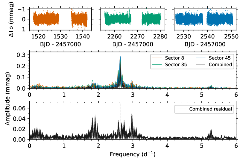
Figure 1: Top panels: TESS light curves for sectors 8, 35 and 45. Middle panel: Amplitude spectra of each TESS sector and all three sectors combined. Bottom panel: Residual amplitude spectrum of all three combined sectors after the dominant frequency has been removed.

3 The ultraviolet variability of $\alpha$ Sex

Nine high resolution SWP and LWP spectra of $\alpha$ Sex were obtained with the International Ultraviolet Explorer from 24 to 27 December 1992 through the large apertures in the frame of program NA026 (PI: Richard Monier). These spectra are calibrated into absolute fluxes, their resolving power is about 25000 and their signal-to-noise ratios is typically a 10-20. They were retrieved from the MAST, and they are collected in Table 2.

Table 2: Log of IUE OBSERVATIONS

Spectrum	Observation	Resolution	Observation	Exposition	FES
	Date		time	Time [s]	counts
SWP 46576	1992-12-24	High	13:47:20	390	3587
LWP 24572	1992-12-24	High	13:59:05	180	3696
SWP 46577	1992-12-24	High	16:12:40	1200	3632
LWP 24573	1992-12-24	High	16:27:19	390	3841
SWP 46584	1992-12-25	High	15:56:55	1200	3321
LWP 24589	1992-12-25	High	16:25:57	4200	3227
SWP 46598	1992-12-27	High	10:14:56	1800	5407
LWP 24605	1992-12-27	Low	11:05:42	420	5542
LWP 24606	1992-12-27	High	12:50:53	420	5443
SWP 46599	1992-12-27	High	16:46:54	600	5401

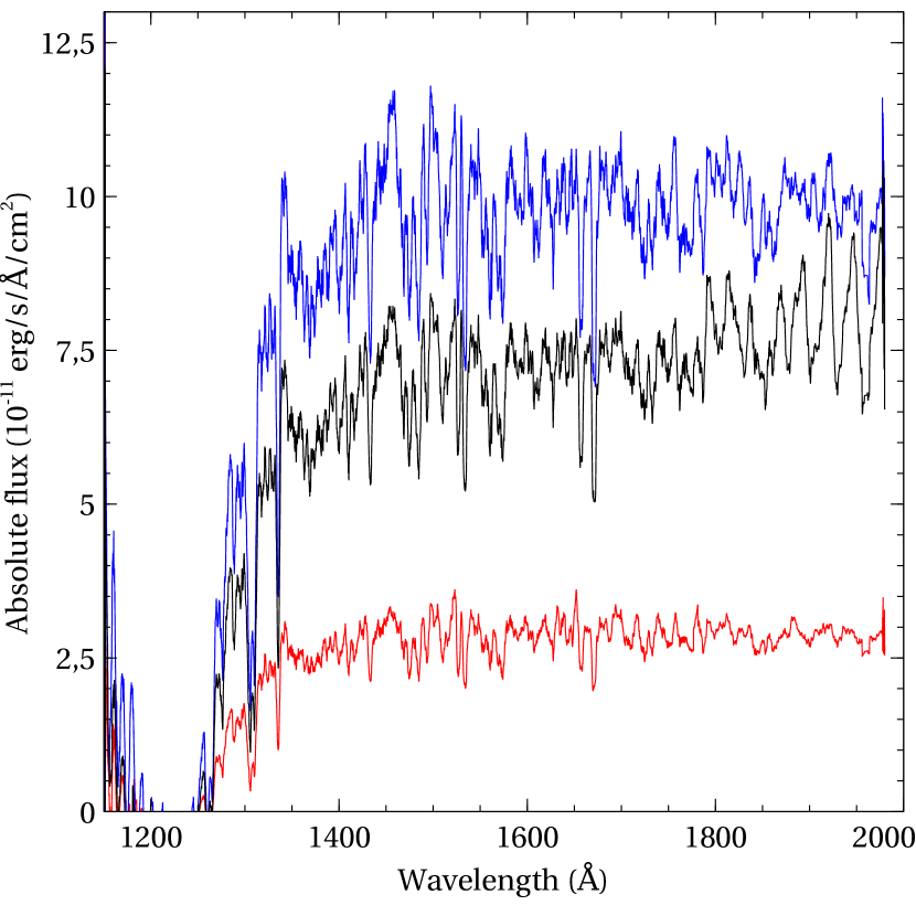
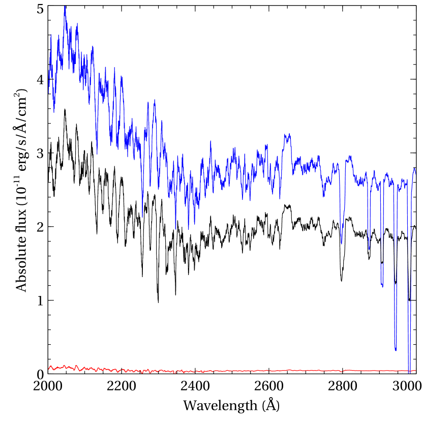
Figure 2: Left: The far UV flux variations of $\alpha$ Sex (SWP 46599, FUV max in blue; SWP 46577 FUV min in red), Right: The mid UV flux variations (LWP 24606: midUV max in blue; LWP2 4589: midUV min in red).

These spectra have been degraded to a lower resolution of about 7 Å comparable to the IUE low resolution in order to highlight the variations. The large variations in the far and mean ultraviolet are shown in Figure 2. In the far UV, four pseudo continuuum windows (regions free of strong lines) are present at 1284, 1342, 1457 and 1756 Å. The ratio of maximum (SWP 46599) to minimum flux (SWP 46577) is about the same in these three windows: 1.35 $\pm$ 0.03. In the mean UV, two windows are observed at 2047 and 2650 Å, where the ratio is about 1.38 $\pm$ 0.01, discarding the spectrum with very low flux LWP 24589. Including this spectrum, the ratio becomes 44 at 2047 Å and 57 at 2650 Å. Before each of these observations, the brightness of $\alpha$ Sex was monitored with the Fine Error Sensor in a broad spectral band near 5000 Å. The FES counts do folllow the UV flux variations: they are larger on December 27 (around 5450 counts) , minimum on December 25 (around 3270 counts) and intermediate on December 24 (around 3690 counts) which means that the UV flux varied in phase with the brightness of the star at 5000 Å. At ultraviolet maximum, the lines in SWP 46599 are consistently redshifted by about 13.7 km s^-1with respect to the spectrum at FUV minimum SWP 46577.

The large diming of the flux by about 70 % at minimum in the far UV compared to the maximum flux could be due to a partial eclipse of $\alpha$ Sex by an hitherto undetected companion. The duration of the eclipse and the shape of the light curve are poorly constrained with the available data, it is therefore difficult to derive information on the radii, temperatures and masses. We can crudely estimate the radius of the secondary star by using the relationship between the flux decrease:

$$\frac{f_{\rm min}}{f_{\rm max}}=\left(\frac{R_{B}}{R_{A}}\right)^{2}$$ (1)

and the radii $R_{A}$ of $\alpha$ Sex and $R_{B}$ of the putative companion. Assuming a radius of about 3.0 $R_{\odot}$ for $R_{A}$ (see section 3), this yields a radius $R_{B}$ close to 2.5 $R_{\odot}$. If the system is indeed eclipsing, it is seen edge-on ($i=\frac{\pi}{2}$). We can estimate a rotation period of 7 days and 19 hours by using the projected equatorial velocity and the estimated radius in section 6 where we discuss the evolutionary status of $\alpha$ Sex. Since no eclipse is seen in the current TESS data, we can place a lower limit on the orbital period of about 28 days, which means that the semi-major axis of the ellipse must be large. Eggleton & Tokovinin (2008) mentioned that $\alpha$ Sex could be a binary, presumably with a long period. Kervella et al. (2019) also think that $\alpha$ Sex may be a binary system considering the renormalised unit weight error from Gaia DR2. Note that the large ultraviolet variations we observe for $\alpha$ Sex do not resemble those of $\delta$ Scuti observed by Monier (1991) throughout its pulsation cycle. The ultraviolet variations of $\delta$ Scuti have modest amplitudes which increase towards shorter wavelengths as expected for a change in effective temperature during the pulsation cycle. This is not the trend we observe for $\alpha$ Sex for which the amplitude of the flux variations does not increase towards shorter wavelengths (the far and mid-UV fluxes vary by a similar amount with time).

4 The abundance pattern of $\alpha$ Sex

4.1 Observations

Four I high resolution profiles (R = 65000) of $\alpha$ Sex have been fetched from the Polarbase archive. These profiles were acquired on 10 May 2018 with the spectropolarimeter NARVAL (Petit et al., 2014) installed at the 2 meter TBL at Pic du Midi Observatory. NARVAL is a cross-dispersed échelle spectrograph mounted on a bench and fed with a fiber from a Cassegrain-mounted polarimeter unit with a wavelength coverage of 3690 up to 10480 Å. The individual I profiles which have a signal-to-noise ratio of 200 around 5000 Å were coadded into a mean spectrum of signal-to-noise of 350. This final spectrum has been sliced into 200 Å wide intervals which were then normalised to a continuum by fitting a cubic spline through narrow regions free of absorption lines.

4.2 Fundamental parameters

The effective temperature ($T_{\mathrm{eff}}$) and surface gravity ($\mathrm{log}\ g$) of $\alpha$ Sex were determined using the UVBYBETA code developed by Napiwotzki et al. (1993). This code is based on the Moon et al. (1985) grid, which calibrates the $uvby\beta$ photometry in terms of $T_{\mathrm{eff}}$ and $\mathrm{log}\ g$. The photometric data was taken from Hauck et al. (1998). The derived effective temperature is $T_{\mathrm{eff}}$= 9950 $\pm$125 K and $\mathrm{log}\ g$= 3.60 $\pm$0.25 dex, respectively (see Sec. 4.2 in Napiwotzki et al. 1993). This value is in good agreement with previous determinations: Adelman (2014) derived $T_{\mathrm{eff}}$= 9875 K from spectrophotometry and the fit to the $H_{\gamma}$ line; McDonald et al. (2012) derived $T_{\mathrm{eff}}$= 9984 K by comparing the spectral energy distribution of $\alpha$ Sex to model atmospheres; and Pintado & Adelman (2004) derived $T_{\mathrm{eff}}$= 9950 K from calibration of uvby$\beta$ photometry.

4.3 Abundance determination

4.3.1 Model atmospheres and spectrum synthesis

The ATLAS9 code (Kurucz, 1992) was used to compute a first model atmosphere for the effective temperature and surface gravity of $\alpha$ Sex assuming a plane parallel geometry, a gas in hydrostatic and radiative equilibrium and local thermodynamical equilibrium. The ATLAS9 model atmosphere contains 72 layers with a regular increase in $\log\tau_{\rm Ross}=0.125$ and was calculated assuming a solar chemical composition (Grevesse et al., 1998). It was converged up to $\log\tau=-5.00$ in order to attempt reproduce the cores of the Balmer lines. This ATLAS9 version uses the new opacity distribution function (ODF) of Castelli et al. (2003) computed for that solar chemical composition. Once a first set of elemental abundances was derived using the ATLAS9 model atmosphere, the atmospheric structure was recomputed for these abundances using the Opacity sampling ATLAS12 code (Kurucz, 2005, 2013). New slightly different abundances were then derived and a new ATLAS12 model recomputed until the abundances of iteration (n-1) differed of those of iteration (n) by less than $\pm$ 0.10 dex.

The abundances of nineteen chemical elements have been derived by iteratively adjusting synthetic spectra to the normalized spectra and looking for the best fit to carefully selected unblended lines. Specifically, synthetic spectra were computed assuming LTE using Hubeny et al. (1992) SYNSPEC49 code which computes lines for elements up to Z=99. The synthetic spectra were further convolved with a rotation parabolic profile for $v_{{\mathrm{e}}}\sin i$ = 21 km s^-1(Abt et al., 2002) and the appropriate FWHM of the instrumental profile of NARVAL. The projected equatorial velocity has been checked by modeling the Fe II lines in the range 4500-4550 Å, they all yield a $v_{{\mathrm{e}}}\sin i$ of about 20.0 $\pm$ 1.0 km s^-1which agrees well with the value provided by Royer et al. (2002). In order to derive the microturbulenct velocity of $\alpha$ Sex, we simultaneously derived the iron abundance [Fe/H] for 50 unblended Fe II lines and a set of microturbulent velocities ranging from 0.0 to 2.0 km s^-1. The adopted microturbulent velocity, $\xi_{t}=1.5$ km s^-1, minimizes the standard deviations, i.e. for that value all Fe II lines yield a similar iron abundance.

We used only unblended lines to derive the abundances. A grid of synthetic spectra was computed with SYNSPEC49 (Hubeny et al., 1992) to model each selected unblended line of the nineteen elements for $\alpha$ Sex. For each modeled transition, the adopted abundance is that which provided the best fit calculated with SYNSPEC49 to the observed normalized profile. Computations were iterated varying the unknown abundance until minimization of the $\chi^{2}$ between the observed and synthetic spectrum was achieved over the spectral range limited to $\pm$ 1.5 Å from the line center. The selected lines are well separated from their neighbours allowing to place the continuum properly on both wings of the line. For a given element, the final abundance is a weighted mean of the abundances derived for each transition (the weights are derived from the NIST grade assigned to that particular transition).

5 Abundance determinations and line identifications for $\alpha$ Sex

The determined abundances for $\alpha$ Sex, expressed relative to hydrogen as $\log(n_{X})-12.0$ (adopting $\log(n_{H})=12.0$) and their errors (standard deviations) are collected in Table 3. Solar abundances are taken from Grevesse et al. (2007). We find that the abundances of $\alpha$ Sex are close to the solar composition.

Helium, nitrogen, oxygen, magnesium, aluminium, silicon, phosphorus, sulfur, calcium, scandium, chromium, manganese, iron and nickel have solar abundances. Only carbon and strontium are underabundant. Titanium, vanadium and baryum are mildly overabundant. The final synthetic spectrum allows to identify most of the lines which absorb more than 2% of the local continuum. It is compared to the observed spectrum in the range 4500 to 4550 Å in Fig. 3. The identifications of these lines are collected in Table LABEL:tab:ident where $E_{\rm low}$ is the energy of the lower excitation level involved in the transition.

Table 3: Elemental abundances and their errors for $\alpha$ Sex

Element	Solar abundance	Absolute abundance	Error
He	-1.07	-1.07	0.32
C	-3.61	-3.37	0.09
N	-4.22	-4.39	0.20
O	-3.34	-3.31	0.19
Mg	-4.47	-4.50	0.08
Al	-5.63	-5.37	0.20
Si	-4.49	-4.49	0.18
P	-6.64	-6.64	0.16
S	-4.86	-4.86	0.11
Ca	-5.69	-5.71	0.05
Sc	-8.83	-9.10	0.28
Ti	-7.10	-6.80	0.13
V	-8.00	-7.60	0.08
Cr	-6.36	-6.36	0.05
Mn	-6.61	-6.57	0.11
Fe	-4.55	-4.69	0.10
Ni	-5.97	-5.99	0.13
Sr	-9.08	-9.23	0.09
Ba	-9.83	-9.34	0.19

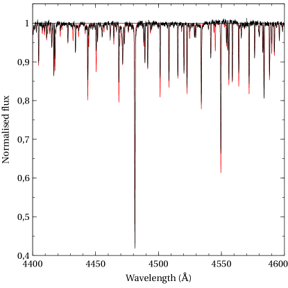
Figure 3: Comparison of the observed mean spectrum of HD 87887 (in black) and the synthetic spectrum (in red) in the range 4500-4550 Å

6 The evolutionary status of $\alpha$ Sex

6.1 Estimations of mass, radius, and evolutionary stage

To estimate the mass, radius, and age of the star, we used the SPInS stellar model optimization tool (Lebreton & Reese, 2020). SPInS uses a Bayesian approach to find the probability distribution function of stellar parameters from a set of constraints. At the heart of the code is a Markov Chain Monte Carlo sampler coupled with interpolation within a pre-computed stellar model grid. Here, we used the BaSTI-IAC grid of stellar models (Hidalgo et al., 2018). This grid is for a solar-scaled heavy element distribution with the solar mixture taken from Caffau et al. (2011) complemented by Lodders (2010), which corresponds to $(Z/X)_{\odot}=0.0209$. The grid considers convective core overshooting included as an instantaneous mixing between Schwarzschild’s convective limit up to layers at a distance $\alpha_{\mathrm{ov}}=0.2H_{P}$ from it, where $H_{P}$ is the pressure scale height at the Schwarzschild limit. Microscopic diffusion is not taken into account. In the calculation process, SPInS can incorporate various priors on the initial mass function (IMF), stellar formation rate (SFR) and metallicity distribution function (MDF). Here we took Kroupa et al. (2013) as IMF and no priors on the SFR and MDF.

With the observational constraints for HD 87887 derived in Sects. 4 and 5 ($T_{\mathrm{eff}}=9950\pm 125\,\mathrm{K},\log g=3.60\pm 0.25$ dex and $\mathrm{[Fe/H]}=-0.14\pm 0.10$), SPInS provided as mean values an age $A=385\pm 77\,\mathrm{Myr}$, a mass $M=2.57\pm 0.32\,M_{\odot}$, a radius $R=3.07\pm 0.90\,R_{\odot}$, a mean density $\overline{\rho}\simeq 0.13\pm 0.11\,\mathrm{g\,cm^{-3}}$, and a luminosity $L=90\pm 52\,L_{\odot}$. The observed position of the star in the Kiel diagram is provided in Fig. 4 together with the isochrones for the $\pm 1\sigma$ age-values inferred by SPInS showing that the star evolves at the vicinity of the main sequence turn-off. We can compare the inferred radius with the observed one using the Swihart et al. (2017)’s angular diameter obtained by interferometry, $\theta\simeq 0.361\pm 0.065$ mas, and parallax values from the literature, that is $\varpi_{\mathrm{G}}=7.66\pm 0.37$ mas (Gaia Collaboration, 2020, Gaia DR3) and $\varpi_{\mathrm{H}}=11.51\pm 0.98$ mas (van Leeuwen, 2007, Hipparcos). This leads to linear radius values of $R_{\mathrm{G}}\simeq 5.1\pm 1.2\,R_{\odot}$ and $R_{\mathrm{H}}\simeq 3.4\pm 0.9\,R_{\odot}$, respectively, such that $R_{\mathrm{H}}$ is closer to our inferred radius rather than $R_{\mathrm{G}}$. To assess our results, we also attempted to derive the stellar parameters using absolute magnitude and a color index in SPInS instead of the $T_{\mathrm{eff}}$ and $\log g$ values derived previously. From the Hipparcos and Tycho-2 constraints on $\varpi_{\mathrm{H}},V_{T}=4.474\pm 0.003$ mag and $(B-V)_{T}=-0.030\pm 0.004$ mag (Høg et al., 2000), we found an age $A=350\pm 25\,\mathrm{Myr}$, a mass $M=2.87\pm 0.12\,M_{\odot}$, and a radius $R=3.66\pm 0.34\,R_{\odot}$, all compatible with our results. On the other hand, we could not find a solution when using the absolute Gaia G-magnitude and (BP-RP) color index, which may indicate difficulties with the Gaia parallax. Indeed, the Gaia-DR3 parallax of $\alpha$ Sex should be taken with care for three reasons: (i) the star is bright; (ii) the astrometric excess noise of the source is around $2$ mas; and (iii) it is a member of a binary system (Kervella et al., 2019).

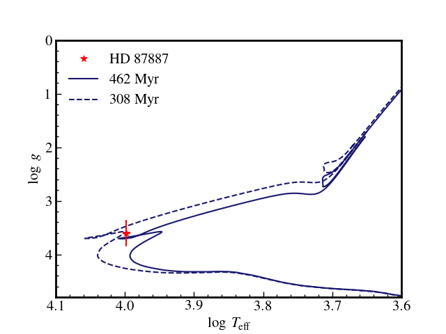
Figure 4: Kiel diagram showing the observed position of HD 87887 together with two isochrones computed for the $\pm 1\sigma$ age-values inferred by SPInS.

7 Discussion and Conclusions

To place the detected variability caused by pulsations in an evolutionary context, we calculate the expected period of the fundamental radial pressure mode of $\alpha$ Sex using its derived parameters. Following Ledoux (1945), we estimate the period of the fundamental radial pressure mode of $\alpha$ Sex to be:

$$P=\left(\frac{3\pi}{G\overline{\rho}}\times\frac{1}{3\Gamma_{1}-4}\right)^{\frac{1}{2}}~{},$$ (2)

assuming the adiabatic exponent is constant throughout the star. For an ideal monoatomic gas for which $\Gamma_{1}\approx 5/3$, this yields $\nu=2.6\pm 1.1$ d^-1 (i.e. $P=9.3\pm 4.1$ hours). This estimate is analogous and compatible with that of the empirical $Q=P\sqrt{\frac{\rho}{\rho_{\odot}}}$ relation for radial pressure modes in $\delta$ Sct stars (Breger & Bregman, 1975), in which $Q=0.033$ for fundamental radial pressure modes. Our estimates are entirely consistent with the observed dominant frequency in the TESS light curve of $\alpha$ Sex. Therefore, we conclude that the observed variability is low-radial order p-mode pulsations. Given its advanced evolutionary stage, it is possible that the observed pulsation modes are of mixed pressure- and gravity-mode character (Aerts et al., 2010). However, future forward asteroseismic data based on much longer light curves with higher duty cycle are needed to confirm this.

Although the pulsations observed in the TESS light curve of $\alpha$ Sex may at first glance appear to resemble the frequency spectra of slowly pulsating B (SPB) stars (e.g. Bowman et al. 2019; Sharma et al. 2022), we present several reasons why this is not the case. SPB stars are mid-to-late B-type dwarf stars and hence hotter and less evolved than $\alpha$ Sex. Moreover, SPB stars are typically fast rotators (Pedersen et al., 2021) and $\alpha$ Sex is not. Indeed, $\alpha$ Sex does not have the characteristic flat-bottomed Fe II lines that Vega has, which is a fast rotator seen pole-on (Hill et al., 2010). If, for example, $\alpha$ Sex were an SPB star and lies within an extension of the SPB stars towards cooler temperatures and lower gravities, it would need to be pulsating in gravity or perhaps Rossby modes (for which the restoring force is the Coriolis force) rather than pressure modes. However, the low $v\,\sin\,i$ combined with $i\simeq 90$ degrees given that the system is eclipsing based on the indicative UV photometry eclipse, makes $\alpha$ Sex unlikely to have gravito(inertial) modes. This is because the frequencies of slowly rotating SPB pulsators are not as high as 2.5 c/d as seen in the TESS light curve of $\alpha$ Sex (see e.g. Pedersen et al. 2021). For gravity-mode frequencies to be so high in such a star, the impact of the Coriolis force would also need to be large, thus $\alpha$ Sex would need to be rapidly rotating. Finally, gravity modes are unlikely to exist above the fundamental radial pressure mode frequency that we derive in this work. Hence we conclude low-radial order pressure and/or mixed modes are the most likely identification of the pulsations based on the fundamental parameters of $\alpha$ Sex derived in this work.

On the issue of whether pressure mode pulsations are expected in a star such as $\alpha$ Sex, we refer to Bowman & Kurtz (2018) and Murphy et al. (2019). In these studies of thousands of $\delta$ Sct stars observed by the Kepler space telescope, the observational hot edge of the classical instability strip was determined to correspond to $T_{\rm eff}\simeq 9000$ K based on the density of such stars in the Kiel and HR diagrams. However, there exist a non-negligible number of outliers with hotter $T_{\rm eff}$ values. Pulsation excitation models struggle to explain the observed pulsations in such stars, because the heat-engine ($\kappa$) mechanism is inefficient at these temperatures (Dupret et al., 2004). Indeed, other pulsation excitation mechanisms operate in delta Scuti stars. Antoci et al. (2014) and Antoci et al. (2019) describe the role of turbulent pressure in the excitation of pulsations in $\delta$ Scuti stars, but such a mechanism typically excites high-radial order and thus high-frequency pressure modes. The discovery of pulsations in $\alpha$ Sex make it an interesting case study for follow-up asteroseismic modeling. Further monitoring with TESS may confirm the presence of eclipses too.

Table 4: Line identifications for $\alpha$ Sex

$\lambda_{\mathrm{obs}}$ (Å)	$\lambda_{\mathrm{lab}}$ (Å)	Species	$\log gf$	$E_{low}$	Ref.
3900.44	3900.55	Ti II	-0.45	9118.260	VALD
3903.78	3903.76	Fe II	-1.49	60807.23	VALD
3905.97	3906.04	Fe II	-1.83	44929.549	VALD
3913.47	3913.47	Ti II	-0.53	8997.710	VALD
3914.56	3914.50	Fe II	-4.05	13474.411	VALD
3917.28	3917.32	Mn II	-1.15	55759.270	VALD
3918.32	3918.30	Fe II	-3.63	73054.879	VALD
3918.76	3918.77	Fe II	-2.30	79246.171	VALD
3920.59	3920.64	Fe II	-1.330	60628.698	VALD
3923.43	3923.46	S II	0.440	130641.115	VALD
3924.953	3924.842	Fe II	-1.100	78138.990	VALD
3926.527	3926.416	Mn II	-1.600	55759.270	VALD
3930.28	3930.30	Fe I	-1.490	704.007	VALD
3933.71	3933.66	Ca II	0.13	0.000	VALD
3936.07	3935.96	Fe II	-1.720	44915.056	VALD
3938.29	3938.29	Fe II	-4.100	13474.447	VALD
3939.02	3938.97	Fe II	-1.930	47674.729	VALD
3941.18	3941.231	Mn II	-2.430	43852.362	VALD
3943.84	3943.86	Mn II	-2.260	43699.122	VALD
3947.33	3947.30	O I	-2.100	73768.202	VALD
3990.95	3990.91	S II	-0.50	128233.19	VALD
3993.52	3993.50	S II	-0.82	115285.608	VALD
3995.04	3995.00	N II	0.28	149187.803	VALD
4002.42	4002.54	Fe II	-2.070	48038.381	VALD
4009.34	4009.26	He I	-1.47	171134.998	VALD
4012.53	4012.50	Cr II	-0.89	45669.369	VALD
4024.67	4024.552	Fe II	-2.400	36252.930	VALD
4026.26	4026.18	He I	-2.62	169086.769	hfs
	4026.19	He I	-0.70	169086.867
	4026.19	He I	-1.45	169086.769
	4026.20	He I	-0.98	169086.845
	4026.20	He I	-0.98	169086.845
4032.94	4032.940	Fe II	-2.570	36254.622	VALD
4045.85	4045.81	Fe I	0.280	11976.239	VALD
4048.86	4048.83	Fe II	-2.380	44917.017	VALD
4057.43	4057.46	Fe II	-1.680	58668.776	VALD
4061.80	4061.78	Fe II	-2.650	48039.087	VALD
4063.60	4063.60	Fe I	0.060	12560.934	VALD
4067.06	4067.03	Ni II	-1.830	32496.075	VALD
4075.63	4075.62	Cr II	-3.470	25035.399	VALD
4081.39	4081.44	Mn II	-2.190	49288.543	VALD
4111.85	4111.88	Fe II	-2.670	48038.381	VALD
4119.62	4119.62	Fe II	-2.690	90780.019	VALD
4120.86	4120.81	He I	-1.740	169086.867	hfs
	4120.82	He I	-1.960	169086.943
	4120.99	He I	-2.430	169087.931
4122.63	4122.67	Fe II	-3.300	20830.553	VALD
4124.67	4124.61	Fe II	-4.200	20516.953	VALD
4128.06	4128.07	Si II	0.360	79338.502	VALD
4130.78	4130.872	Si II	-0.780	79355.019	VALD
	4130.89	Si II	0.550	79355.019	VALD
4136.90	4136.902	Mn II	-1.250	49514.374	VALD
4143.90	4143.76	He I	-1.200	179134.998	VALD
4162.63	4162.67	S II	0.780	128599.162	VALD
4163.54	4163.65	Ti II	-0.130	20891.790	VALD
4164.92	4164.92	Fe III	1.010	198821.396	VALD
4167.21	4167.30	Fe II	-0.560	90300.626	VALD
4169.04	4168.97	He I	-2.340	171134.998	VALD
4171.02	4171.03	Mn II	-2.340	49425.654	VALD
4171.85	4171.903	Cr II	-2.940	25043.517	VALD
	4171.904	Ti II	-0.290	20951.754	VALD
4173.46	4173.46	Fe II	-2.160	20830.553	VALD
4174.17	4174.27	S II	0.800	140319.232	VALD
4175.97	4175.99	Fe II	-3.840	54902.315	VALD
4178.61	4178.63	Fe II	-4.290	60402.341	VALD
4199.39	4199.49	Fe II	-0.330	89922.758	VALD
4200.47	4200.518	Fe II	-0.410	90067.932	VALD
4205.38	4205.38	Mn II	-3.450	14593.834	VALD
4206.44	4206.37	Mn II	-1.540	43528.661	VALD
4233.12	4233.17	Fe II	-1.810	20830.553	VALD
4239.05	4239.15	Mn II	-2.240	43311.972	VALD
4242.33	4242.33	Mn II	-1.260	49820.865	VALD
	4242.36	Cr II	-1.170	31221.723	VALD
4244.46	?
4246.85	4246.82	Sc II	0.240	2540.950	VALD
4250.43	4250.44	Fe II	-1.720	61974.931	VALD
4251.64	4251.72	Mn II	-1.060	49885.389	VALD
4252.97	4252.96	Mn II	-1.140	49893.458	VALD
4258.17	4258.11	Fe II	-3.500	21812.044	VALD
4259.17	4259.17	Mn II	-1.440	43537.186	VALD
4261.92	4261.91	Cr II	-1.340	31165.263	VALD
4263.81	4263.87	Fe II	-1.690	62048.230	VALD
4267.15	4267.18	C II	0.720	145550.705	VALD
4273.26	4273.33	Fe II	-3.300	21812.044	VALD
4278.29	4278.15	Fe II	-3.950	21712.445	VALD
4286.17	4286.16	Fe III	0.700	184316.573	VALD
4288.05	4288.07	Mn II	-2.760	43311.301	VALD
4290.25	4290.22	Ti II	-0.850	9395.802	VALD
4292.17	4292.23	Mn II	-1.540	43395.394	VALD
4294.18	4294.10	Ti II	-1.110	8744.341	VALD
4296.57	4296.57	Fe II	-2.900	21812.044	VALD
4300.18	4300.04	Ti II	-0.440	9518.152	VALD
4303.10	4303.18	Fe II	-2.610	21812.044	VALD
4307.92	4307.87	Ti II	-1.070	9395.802	VALD
4312.98	4312.85	Ti II	-1.100	9518.152	VALD
4314.24	4314.31	Fe II	-3.600	21583.397	VALD
4320.92	4320.96	Ti II	-1.800	9395.802	VALD
4325.44	4325.44	Fe II	-2.380	49506.310	VALD
	4325.53	Fe II	-2.360	49103.030	VALD
4326.59	4326.64	Mn II	-1.370	43537.186	VALD
4351.70	4351.76	Fe II	-2.080	21812.044	VALD
4354.39	4354.34	Fe II	-1.350	61725.611	VALD
4357.61	4357.58	Fe II	-2.010	49100.956	VALD
4361.15	4361.25	Fe II	-2.260	49506.310	VALD
4363.16	4363.26	Mn II	-1.890	44900.887	VALD
4365.20	4365.22	Mn II	-1.340	53014.822	VALD
4368.21	4368.242	O I	-1.960	76794.977	VALD
	4368.250	O I	-2.190	76794.977	VALD
4369.42	4369.400	Fe II	-3.600	22409.818	VALD
4374.71	4374.82	Ti II	-1.290	16625.110	VALD
4377.61		?
4379.62	4379.67	Mn II	-1.870	43852.362	VALD
4382.51	4382.51	Fe III	-3.020	66522.952	VALD
4384.40	4384.32	Fe II	-3.700	21430.357	VALD
4385.35	4385.39	Fe II	-2.600	22409.818	VALD
4388.04	4387.93	He I	-0.887	171134.897	VALD
4390.55	4390.514	Mg II	-1.480	80650.022	VALD
	4390.564	Mg II	-0.520	80650.022	VALD
4395.04	4395.031	Ti II	-0.660	8744.341	VALD
4395.83	4395.76	Fe III	-2.600	66591.679	VALD
4402.92	4402.879	Fe II	-2.600	49506.924	VALD
4404.87	4404.75	Fe I	-0.140	12560.934	VALD
4407.74	4407.68	Fe II	0.780	109473.634	VALD
4409.54	4409.53	Fe II	0.950	109489.771	VALD
4411.14	4411.072	Ti II	-0.670	24961.191	VALD
	4411.15	C II	0.530	198425.425	VALD
4413.62	4413.60	Fe II	-4.200	21581.615	VALD
4416.81	4416.83	Fe II	-2.600	22409.818	VALD
4417.70	4417.71	Ti II	-1.430	9395.802	VALD
4418.73	4418.78	Ce II	0.180	6967.547	VALD
4419.56	4419.60	Fe III	-2.210	66468.153	VALD
	4419.60	Cr II	-0.260	94365.189	VALD
4428.01	4427.99	Mg II	-1.210	80619.500	VALD
4430.99	4431.02	Fe III	-2.570	66522.952	VALD
4434.00	4433.99	Mg II	-0.910	80650.022	VALD
4437.58	4437.55	He I	-2.030	171134.998	VALD
4443.81	4443.79	Ti II	-0.720	8710.567	VALD
4451.49	4451.55	Fe II	-1.910	49506.924	VALD
4455.33	4455.27	Fe II	-2.000	50216.076	VALD
4461.65	4461.71	Fe II	-2.100	50212.834	VALD
4463.43	4463.41	Ce II	-0.110	7722.285	VALD
4464.46	4464.45	Ti II	-2.080	9363.620	VALD
4468.51	4468.51	Ti II	-0.620	9118.285	VALD
4469.93	4469.90	Mn II	-3.170	49882.153
4471.46	4471.470	He I	-2.210	169086.769	hfs
	4471.474	He I	-1.040	169086.769
	4471.474	He I	-0.240	169086.769
	4471.486	He I	-1.040	169086.769
	4471.489	He I	-0.560	169086.769
4472.73	4472.62	Fe II	-2.340	61974.931
4478.67	4478.64	Mn II	-0.940	53595.541	VALD
4481.21	4481.130	Mg II	0.750	71490.190	VALD
	4481.150	Mg II	-0.550	71490.190	VALD
	4481.327	Mg II	0.590	71491.058	VALD
4483.49	4483.43	S II	-0.320	128233.197	VALD
4489.19	4489.19	Fe II	-3.000	22810.345	VALD
4491.37	4491.40	Fe II	-2.640	23031.283	VALD
4493.47	4493.53	Fe II	-1.560	63876.325	VALD
4494.41	4494.42	Zr II	-0.480	19433.239	VALD
4501.24	4501.27	Ti II	-0.770	8997.787	VALD
	4501.28	Fe II	-0.950	90387.870	VALD
4515.39	4515.34	Fe II	-2.360	22939.352	VALD
4518.91	4518.96	Mn II	-1.310	53595.541	VALD
4520.15	4520.22	Fe II	-2.600	22637.195	VALD
4522.57	4522.63	Fe II	-1.990	22939.352	VALD
4524.87	4524.94	S II	0.030	121530.021	VALD
4526.50	4526.40	Fe II	-2.330	62962.204	VALD
4529.28	?
4534.00	4533.97	Ti II	-0.770	9975.999	VALD
4541.45	4541.52	Fe II	-3.000	23031.283	VALD
4549.39	4549.47	Fe II	-1.730	22810.345	VALD
4552.47	4552.41	S II	-0.100	121528.718	VALD
4555.01	4554.99	Cr II	-1.370	32836.653	VALD
4555.86	4555.89	Fe II	-2.250	22810.345	VALD
4558.61	4558.64	Cr II	-0.660	32854.249	VALD
4563.69	4563.76	Ti II	-0.960	9851.014	VALD
4571.96	4571.97	Ti II	-0.320	12677.106	VALD
4576.34	4576.33	Fe II	-2.920	22939.352	VALD
4579.67	4579.72	Ti II	-1.950	40581.490	VALD
4582.69	4582.84	Fe II	-3.060	22939.352	VALD
4583.81	4583.84	Fe II	-1.740	22637.195	VALD
4588.12	4588.20	Cr II	-0.640	32836.653	VALD
4589.87	4589.95	Ti II	-1.780	9975.999	VALD
4595.95	4596.02	Fe II	-1.960	50212.834	VALD
4598.43	4598.49	Fe II	-1.540	62945.045	VALD
4616.63	4616.63	Cr II	-1.290	32844.706	VALD
4618.79	4618.81	Cr II	-1.110	32854.941	VALD
4620.50	4620.51	Fe II	-3.190	22810.345	VALD
4621.51	4621.40	N II	-0.540	148940.167	VALD
4625.70	4625.64	C II	0.700	199941.414	VALD
4629.31	4629.29	Ti II	-2.250	9518.152	VALD
	4629.332	Fe II	-2.260	22637.195	VALD
4634.09	4634.07	Cr II	-1.240	32844.706	VALD
4635.21	4635.32	Fe II	-1.580	48039.109	VALD
4638.05	4638.04	Fe II	-1.540	62169.219	VALD
4656.90	4656.98	Fe II	-3.570	23317.635	VALD
4663.34	?
4713.31	4713.38	He I	-1.920	169087.931	VALD
4716.40	4716.267	S II	-0.370	109831.595	VALD
4727.92	4727.84	Mn II	-1.950	43311.972	VALD
4730.37	4730.40	Mn II	-2.020	43336.173	VALD
4731.49	4731.44	Fe II	-3.100	23317.635	VALD
4738.23	4738.29	Mn II	-1.870	43395.394	VALD
4755.72	4755.73	Mn II	-1.220	43529.741	VALD
4764.64	4764.728	Mn II	-1.330	43537.810	VALD
4784.52	4784.63	Mn II	-1.500	53014.822	VALD
4791.82	4791.78	Mn II	-1.680	49885.389	VALD
4806.71	4806.860	Mn II	-1.840	43696.217	VALD
4815.51	4815.55	S II	0.070	110268.595	VALD
	4815.49	Mn II	-3.780	43696.190
4824.11	4824.06	S II	0.180	110268.595	VALD
	4824.13	Cr II	-1.230	31219.331	VALD
4826.53	4826.51	Mn II	-3.000	94230.896
4848.18	4848.24	Cr II	-1.130	31168.575	VALD
4876.37	4876.40	Cr II	-1.460	31084.610	VALD
4883.28	4883.28	Fe II	-0.600	82853.704	VALD
4908.12	4908.15	Fe II	-0.270	83308.242	VALD
4909.75	4909.75	Fe II	-2.610	82978.679	VALD
4911.52	?
4913.29	4913.30	Fe II	0.050	82978.717	VALD
4917.22	4917.21	S II	-0.380	112937.572	VALD
4921.86	?
4923.90	4923.92	Fe II	-1.210	23317.635	VALD
4948.42	4948.49	Mn II	-3.220	62572.200	VALD
4951.58	4951.58	Fe II	0.210	83136.510	VALD
4954.03	4953.98	Fe II	-2.810	44933.149	VALD
4977.02	4977.04	Fe II	-0.040	83558.566	VALD
4984.52	4984.49	Fe II	0.080	83308.242	VALD
	4984.58	Fe II	-1.260	83990.065	VALD
4990.51	4990.51	Fe II	0.200	83308.242	VALD
4991.70	?
4993.38	4993.36	Fe II	-3.700	22637.195	VALD
5001.86	5001.95	Fe II	0.920	82853.704	VALD
5004.19	5004.19	Fe II	0.500	82853.704	VALD
5007.21	?
5009.54	5009.56	S II	-0.230	109831.595	VALD
5014.03	5014.04	S II	0.050	113461.537	VALD
5015.63	5015.68	He I	-0.820	166277.440	VALD
	5015.75	Fe II	-0.030	83459.720	VALD
5018.37	5018.44	Fe II	-1.350	23317.635	VALD
5019.70	?
5021.42	5021.47	Ni II	0.920	100309.295	VALD
5022.60	5022.42	Fe II	-0.070	83459.720	VALD
5026.91	5026.80	Fe II	-0.440	83136.510	VALD
5028.95	5028.98	Ni II	0.170	100389.516	VALD
5030.63	5030.63	Fe II	0.430	82978.717	VALD
5032.58	5032.45	S II	0.190	110268.595	VALD
5034.21	5034.17	Fe II	-0.800	83558.566	VALD
5035.69	5035.71	Fe II	0.630	82978.717	VALD
5036.856	5036.713	Fe II	-0.560	83812.350	VALD
5040.92	5041.02	Si II	0.030	81191.341	VALD
5045.11	5045.11	Fe II	0.000	83136.510	VALD
5047.62	5047.64	Fe II	-0.240	83136.510	VALD
	5047.74	He I	-1.600	171134.198	VALD
5056.07	5055.98	Si II	0.520	81251.320	VALD
5061.74	5061.72	Fe II	0.280	83136.510	VALD
5067.89	5067.890	Fe II	-0.080	83308.242	VALD
5070.90	5070.90	Fe II	0.270	83136.510	VALD
5073.94	5073.896	Fe II	-0.720	84266.595	VALD
	5074.051	Fe II	-2.200	54904.243	VALD
	5073.90	Fe III	-2.560	69788.188	VALD
5075.80	5075.760	Fe II	0.180	84326.965	VALD
5082.10	5082.23	Fe II	-0.130	83990.103	VALD
5087.33	5087.300	Fe II	-0.420	83713.585	VALD
	5087.419	Y II	-0.170	8743.050	VALD
5089.25	5089.21	Fe II	0.010	83308.242	VALD
5093.62	5093.58	Fe II	-2.320	54869.899	VALD
5097.19	5097.27	Fe II	0.320	83713.585	VALD
5098.70	5098.68	Fe II	-0.490	84268.805	VALD
5100.71	5100.73	Fe II	0.720	83726.416	VALD
5102.54	5102.52	Mn II	-1.900	48320.677	VALD
5106.12	5106.11	Fe II	-0.250	83308.242	VALD
5107.33	5107.25	Fe II	-3.960	50075.908	VALD
5116.99	5117.031	Fe II	-0.040	84131.623	VALD
5123.31	5123.33	Mn II	-1.850	48336.810	VALD
5127.53	5127.63	Fe III	-2.560	69837.758	VALD
5129.96	?
5132.58	5132.66	Fe II	-4.100	22637.195	VALD
5133.97	5134.07	Fe II	0.290	104916.599	VALD
5144.28	5144.32	Fe II	0.310	84424.421	VALD
5145.85	5145.730	Fe II	-0.210	83990.103	VALD
	5145.822	Fe II	-0.140	83990.103	VALD
5149.25	5149.19	Fe II	0.410	103601.919
5152.850	5152.88	Fe II	-0.990	83990.065	VALD
5154.24	?
5156.31	5156.28	Fe II	-3.750	93487.649
5157.40	5157.28	Fe II	-0.170	84326.965	VALD
5160.83	5160.840	Fe II	-2.600	44915.056	VALD
5163.37	?
5166.17	5166.20	Fe II	0.930	108134.747	VALD
5168.92	5169.03	Fe II	-0.870	23317.635	VALD
5170.49	?
5172.97	5173.13	Fe II	0.460	105061.784	VALD
5177.37	5177.37	Fe II	1.160	103642.253	VALD
5180.21	5180.31	Fe II	-0.090	83812.350	VALD
5183.57	5183.53	Fe II	-0.850	84131.564	VALD
5188.80	5188.687	Ti II	-1.220	12758.260	VALD
5189.96	5190.00	Fe II	0.490	105400.535	VALD
5192.70	5192.62	Fe II	0.200	103101.857	VALD
5196.01	5195.94	Fe II	0.920	104174.580	VALD
5197.55	5197.57	Fe II	-2.050	26055.412	VALD
5199.00	5199.12	Fe II	0.120	83713.585	VALD
5200.92	5200.80	Fe II	-0.040	83812.350	VALD
	5201.03	S II	0.430	121528.718	VALD
5210.58	5210.550	Fe II	0.790	103166.386	VALD
5212.61	5212.62	S II	0.320	121530.021	VALD
5213.97	5213.95	Fe II	-0.260	84527.806	VALD
	5214.003	Fe II	0.860	104069.717	VALD
5215.48	5215.35	Fe II	0.000	83713.585	VALD
5216.90	5216.86	Fe II	0.670	84527.806	VALD
	5216.859	Fe II	0.480	84710.751	VALD
5218.70	5218.84	Fe II	-0.170	83726.416	VALD
5223.26	5223.20	Fe II	0.450	103876.141	VALD
	5223.260	Fe II	-0.170	83812.350	VALD
5225.26	5225.21	Fe II	0.980	105287.615	VALD
	5225.35	Fe II	0.710	103190.571	VALD
5227.44	5227.32	Fe II	0.190	84844.864	VALD
	5227.49	Fe II	0.850	84296.883	VALD
5228.71	5228.63	Fe II	0.900	108779.995	VALD
5232.76	5232.78	Fe II	-0.080	83726.416	VALD
5234.53	5234.44	Fe II	-2.210	25981.646	VALD
	5236.621	Fe II	-0.680	84326.965	VALD
5237.90	5237.95	Fe II	0.100	84266.595	VALD
5239.62	5239.65	Mn II	-3.430	82419.479
5241.00	5241.06	Fe II	-0.580	83812.350	VALD
5245.11	5245.07	Fe II	0.870	108465.440	VALD
5247.95	5247.96	Fe II	0.550	84938.264	VALD
5251.20	5251.21	Fe II	-0.660	84325.265	VALD
	5251.23	Fe II	0.420	84844.864	VALD
5254.77	5254.920	Fe II	-3.340	26051.708	VALD
5257.02	5256.93	Fe II	-4.180	23317.488	VALD
	5257.12	Fe II	0.160	84685.247	VALD
5258.08	5258.03	Fe II	-2.100	84685.198	VALD
	5258.12	Fe II	-0.920	84424.372	VALD
5260.15	5260.254	Fe II	1.090	84035.172	VALD
5262.462	5262.313	Fe II	-0.370	85048.655	VALD
5264.169	5264.020	Fe II	-0.440	84685.247	VALD
5264.328	5264.179	Fe II	0.300	84710.751	VALD
5264.364	5264.215	Mg II	-0.370	93310.590	VALD
5264.49	5264.36	Mg II	-0.530	93311.112	VALD
5272.38	5272.41	Fe II	-2.010	48039.109	VALD
5274.83	5274.965	Cr II	-1.560	32834.831	VALD
5275.92	5275.997	Fe II	-1.900	25805.326	VALD
5284.02	5284.07	Fe II	-3.200	23317.635	VALD
	5284.11	Fe II	-3.190	23317.632	VALD
5291.67	5291.67	Fe II	0.580	84527.779	VALD
5296.99	5297.000	Mn II	-0.240	79550.458	hfs
	5297.028	Mn II	0.400	79550.458
	5297.060	Mn II	0.620	79550.502
5299.29	5299.302	Mn II	-0.440	79558.533	hfs
	5299.330	Mn II	0.380	79558.533
	5299.370	Mn II	0.830	79558.560
5302.39	5302.402	Mn II	0.200	79566.596	hfs
	5302.440	Mn II	1.000	79569.219
5306.06	5306.18	Fe II	0.040	84870.912	VALD
5308.36	5308.41	Fe II	0.550	104118.119	VALD
	5308.41	Cr II	-1.810	32836.653	VALD
5316.62	5316.61	Fe II	-1.780	25428.789	VALD
5316.78	5316.78	Fe II	-2.800	25981.646	VALD
5318.21	5318.06	Fe II	-0.230	84527.806	VALD
5320.68	5320.72	S II	0.430	121530.021	VALD
5322.01	5321.86	Fe II	0.670	106021.587	VALD
5325.38	5325.543	Fe II	-3.260	25981.646	VALD
5330.78	5330.73	O I	-2.570	86631.453	VALD
	5330.74	O I	-1.570	86631.453	VALD
	5330.740	O I	-0.980	86631.453	VALD
	5330.78	Ne I	-1.040	148257.789
5339.50	5339.594	Fe II	0.520	84296.883	VALD
5362.75	5362.74	Fe II	-0.190	84710.751	VALD
5370.43	5370.28	Fe II	-0.570	84266.595	VALD
5375.83	5375.842	Fe II	-0.330	84296.883	VALD
5375.994	5375.842	Fe II	-0.700	85048.655	VALD
5387.00	5387.06	Fe II	0.500	84863.380	VALD
5393.80	5393.84	Fe II	-0.250	84296.883	VALD
5395.83	5395.86	Fe II	0.280	85495.368	VALD
5401.95	5401.89	Fe II	-0.840	85462.859
5405.14	5405.09	Fe II	-0.430	85172.826	VALD
5411.49	5411.373	Fe II	-0.050	85495.368	VALD
5414.42	?
5427.89	5427.83	Fe II	-1.580	54232.199	VALD
5429.93	5429.987	Fe II	0.430	85462.908	VALD
5432.85	5432.82	S II	0.200	109831.595	VALD
5442.36	5442.359	Fe II	-0.310	85048.655	VALD
5443.80	?
5444.25	5444.39	Fe II	-0.170	85495.368	VALD
5445.67	5445.80	Fe II	-0.110	85048.655	VALD
5455.98	5455.930	Fe II	-0.510	84527.806	VALD
5457.70	5457.72	Fe II	-0.140	85728.844	VALD
5465.91	5465.932	Fe II	0.350	85679.757	VALD
5467.049	5466.894	Si II	-0.080	101024.349	VALD
	5466.912	Fe II	-1.870	54902.288	VALD
5473.15	5473.15	Fe II	-1.440	86844.832	VALD
5475.89	5475.83	Fe II	-0.080	84685.247	VALD
5478.32	5478.365	Cr II	-1.970	33697.843	VALD
	5479.399	Fe II	-0.350	85172.826	VALD
5479.44	5479.40	Fe II	-0.410	87172.810	VALD
5482.22	5482.31	Fe II	0.410	85184.772	VALD
5487.53	5487.62	Fe II	0.290	85462.908	VALD
5492.23	5492.078	Fe II	0.090	85679.757	VALD
5493.91	5493.83	Fe II	0.260	84685.247	VALD
5502.95	?
5506.20	5506.199	Fe II	0.860	84863.380	VALD
5510.87	5510.78	Fe II	0.100	85184.772	VALD
5529.47	5529.47	Cr II	-2.890	97899.412
5532.05	5532.09	Fe II	-0.100	84870.912	VALD
5534.83	5534.839	Fe II	-2.900	26170.181	VALD
	5534.894	Fe II	-0.440	85048.655	VALD
5544.46	?
5549.01	5549.000	Fe II	-0.190	84870.912	VALD
5554.89	5554.910	Fe II	-0.460	85680.279	VALD
5558.94	5559.05	Mn II	-1.310	49885.389	VALD
5561.30	5561.43	Mn II	-2.420	49893.458	VALD
5567.86	5567.84	Fe II	-1.870	54283.234	VALD
5570.49	5570.54	Mn II	-1.430	49820.865	VALD
5577.96	5577.912	Fe II	-0.110	85462.908	VALD
	5578.008	Fe II	-0.620	85495.368	VALD
5586.94	5586.842	Cr II	0.930	88003.158	VALD
5588.21	5588.221	Fe II	0.160	85462.908	VALD
5606.14	5606.15	S II	0.120	110766.562	VALD
5645.47	5645.39	Fe II	0.190	85184.772	VALD
5648.830	5648.90	Fe II	-0.170	85184.772	VALD
5651.40	5651.52	Fe II	-0.610	85728.844	VALD
5660.15	5659.99	S II	-0.220	110313.403	VALD
5726.59	5726.55	Fe II	-0.040	86416.369	VALD
5780.09	5780.13	Fe II	0.420	86124.348	VALD
5783.75	5783.62	Fe II	0.370	86416.369	VALD
5811.73	5811.634	Fe II	-0.610	86124.348	VALD
	5811.79	Fe II	-0.640	86124.299	VALD
5813.59	5813.67	Fe II	-2.700	44929.533	VALD
5842.19	5842.29	Fe II	-0.330	86599.791	VALD
5852.44	5852.49	Ne I	-0.450	135888.715	VALD
5854.12	5854.19	Fe II	-0.110	86599.791	VALD
5871.67	5871.80	Fe II	-0.640	86124.299	VALD
5875.75	5875.599	He I	-1.510	169086.769	hfs
	5875.614	He I	-0.340	169086.769
	5875.615	He I	0.410	169086.769
	5875.615	He I	-0.340	169086.845
	5875.640	He I	0.140	169086.845
	5875.966	He I	-0.210	169087.834
5902.95	5902.83	Fe II	0.420	86416.331	VALD
5961.68	5961.71	Fe II	0.700	86124.299	VALD
5978.85	5978.93	Si II	0.000	81251.320	VALD
6096.19	6096.16	Ne I	-0.300	134459.290	VALD
6122.48	6122.45	Mn II	0.950	82136.483	VALD
6143.04	6143.06	Ne I	-0.100	134041.838	VALD
6147.65	6147.74	Fe II	-2.800	31364.454	VALD
6149.28	6149.26	Fe II	-2.800	31368.453	VALD
6156.57	6155.961	O I	-1.360	86625.757	hfs
	6155.980	O I	-1.010	86625.757
	6155.989	O I	-1.120	86625.757
	6156.737	O I	-1.490	86627.777
	6156.755	O I	-0.900	86627.777
	6156.770	O I	-0.690	86627.777
6158.14	6158.172	O I	-1.000	86631.453	hfs
	6158.180	O I	-0.410	89511.404
6163.69	6163.59	Fe II	-3.170	50157.455	VALD
6175.13	6175.14	Fe II	-2.090	50187.824	VALD
6238.32	6238.39	Fe II	-2.800	31364.454	VALD
6239.65	6239.610	Si II	0.180	103556.025	VALD
	6239.660	Si II	0.020	103556.156	VALD
6247.47	6247.56	Fe II	-2.400	31387.979	VALD
6334.33	6334.43	Ne I	-0.310	134041.838	VALD
6347.00	6346.737	Mg II	0.030	93310.590	VALD
	6346.962	Mg II	-0.130	93311.112	VALD
	6347.100	Si II	0.150	65500.472	VALD
6357.19	6357.16	Fe II	0.240	87985.668	VALD
6371.23	6371.36	Si II	-0.080	65500.472	VALD
6383.22	?
6402.19	6402.25	Ne I	0.350	134041.838	VALD
6416.84	6416.92	Fe II	-2.900	31387.979	VALD
6432.67	6432.68	Fe II	-3.500	23317.635	VALD
	6432.68	Fe II	-3.710	23317.632	VALD
6456.22	6456.38	Fe II	-2.200	31483.198	VALD
6506.56	6506.53	Ne I	0.030	134459.290	VALD
6577.99	6578.05	C II	0.120	116537.649	VALD
6582.92	6582.88	C II	-0.180	116537.649	VALD
6678.10	6678.15	He I	0.329	171134.897	VALD

References

- Abt et al. (2002) Abt, H.A., Levato, H. and Grosso, M. 2002, ApJ, 573, 359
- Adelman (2014) Adelman, S.J. 2014, PASP, 126, 505A
- Aerts et al. (2010) Aerts, C., et al., 2010, Springer, Asteroseismology
- Alecian et al. (2002) Alecian, G. & LeBlanc, F. 2002, MNRAS, 332, 900
- Angulo (1999) Angulo, C. 1999, American Institute of Physics Conference Series, 495, 366
- Antoci et al. (2014) Antoci, A., et al., 2014, ApJ, 796, 118A
- Antoci et al. (2019) Antoci, V., et al., 2019, MNRAS, 490, 4040
- Asplund et al. (2009) Asplund, M., Grevesse, N., Sauval, A. J., et al. 2009, ARA&A, 47, 522
- Bowman & Kurtz (2018) Bowman, D. M. & Kurtz, D. W. 2018, MNRAS, 476, 3169-3184
- Bowman et al. (2019) Bowman, D. M., et al. . 2019, Nature Astronomy, 3, 760-765
- Bowman et al. (2022) Bowman, D. M., Vandenbussche, B., Sana, H., et al. 2022, A&A, 658, A96
- Bowman & Michielsen (2021) Bowman, D. M., Michielsen, M., 2021, A&A, 656, A158
- Breger & Bregman (1975) Breger, M., Bregman, J. N., et al. 1975, ApJ, 200, 343-353
- Breger (2000) Breger, M., 2000, Astronomical Society of the Pacific Conference Series, 210, 3
- Caffau et al. (2011) Caffau, E., Ludwig, H.-G., Steffen, M., et al. 2011, Sol. Phys., 268, 255.
- Canuto et al. (1996) Canuto, V. M., Goldman, I. & Mazzitelli, I. 1996, ApJ, 473, 550
- Castelli et al. (2003) Castelli, F. & Kurucz, R. L. 2003, IAU Symposium, 210, A20
- Deal et al. (2018) Deal, M., Alecian, G., Lebreton, Y., et al. 2018, A&A, 618, A10
- Dupret et al. (2004) Dupret, M. A., et al. 2004, A&A, 414, L17-L20
- Dolk et al. (2003) Dolk, L., Walgren, G.M. and Hubrig, S., et al. 2003, A&A, 402, 299
- Eggleton & Tokovinin (2008) Eggleton, P. P.; Tokovinin, A. A. 2008, MNRAS, 389, 869
- Ferguson et al. (2005) Ferguson, J. W., Alexander, D. R., Allard, F., et al. 2005, ApJ, 623, 596
- Gaia Collaboration (2018) Gaia Collaboration 2018, VizieR Online Data Catalog, I/345
- Gaia Collaboration (2020) Gaia Collaboration 2020, VizieR Online Data Catalog, I/350
- Ghazaryan et al. (2018) Ghazaryan, S., Alecian, G. and Hakobyan, A. A. 2018, MNRAS, 480, 2962
- Gray & Garrison (1987) Gray, R.,O. and Garrison, R.F. 1987, Apjs, 65, 581G
- Grevesse et al. (2007) Grevesse, N., Asplund, M. & Sauval, A.J 2007, Space Sci. Rev., 130, 105
- Grevesse et al. (1998) Grevesse, N. & Sauval, A. J. 1998, Space Sci. Rev., 85, 174
- Hauck et al. (1998) Hauck, B. & Mermilliod, M. 1998, ApJ, 129, 433
- Hidalgo et al. (2018) Hidalgo, S. L., Pietrinferni, A., Cassisi, S., et al. 2018, ApJ, 856, 125.
- Hill et al. (2010) Hill, G., Gulliver, A.F., Adelman, S. J., 2010, ApJ, 712, 250H
- Høg et al. (2000) Høg , E., Fabricius, C., Makarov, V. V., Urban, S., Corbin, T., Wycoff, G., Bastian, U., Schwekendiek, P., Wicenec, A. 2000, A&A, 355, L27
- Hubeny et al. (1992) Hubeny, I. & Lanz, T. 1992, A&A, 262, 514
- Imbriani et al. (2004) Imbriani, G., Costantini, H., Formicola, A. et al. 2005, A&A, 420, 629
- Jenkins et al. (2016) Jenkins, J. M., Twicken, J. D., McCauliff, S. et al. 2016, Proc. SPIE, 9913, 99133E
- Kervella et al. (2019) Kervella, P.; Arenou, F.; Mignard, F.; Thévenin, F., 2019, A&A, 623, 72K
- Kroupa et al. (2013) Kroupa, P., Weidner, C., Pflamm-Altenburg, J., et al. 2013, Planets, Stars and Stellar Systems. Volume 5: Galactic Structure and Stellar Populations, 115. doi:10.1007/978-94-007-5612-0_4
- Kurtz (1985) Kurtz, D. W., 1985, MNRAS, 213, 773-776
- Kurucz (1992) Kurucz, R. L. 1992, Rev. Mexicana Astron. Astrofis., 23
- Kurucz (2005) Kurucz, R. L. 2005, Memorie della Societa Astronomica Italiana Supplementi, 8, 14
- Kurucz (2013) Kurucz, R. L. 2013, Astrophysics Source Code Library
- LeBlanc et al. (2004) LeBlanc, F. & Alecian, G. 2004, MNRAS, 352, 1334
- Lebreton & Reese (2020) Lebreton, Y., Reese, D.R. 2020, A&A, 642, A88
- Ledoux (1945) Ledoux, P. 1945, ApJ, 102, 143.
- Lodders (2010) Lodders, K. 2010, Principles and Perspectives in Cosmochemistry, 16, 379.
- Lightkurve Collaboration (2018) Lightkurve collaboration et al. 2018, ascl:1812.013, https://ui.adsabs.harvard.edu/abs/2018ascl.soft12013L
- Maestro et al. (2013) Maestro, V., Che, X., Huber, D., et al. 2013, MNRAS, 434, 1331
- McDonald et al. (2012) McDonald, I., Zijlstra, A.A. and Boyer M.L. 2012, MNRAS, 427, 343
- Monier (1991) Monier, R., 1991, AJ, 102, 234M
- Monier et al. (2019) Monier, R., Griffin, E. & Kılıçoğlu, T. 2019, Research Notes of the American Astronomical Society, 3, 14
- Moon et al. (1985) Moon, T. T. & Dworetsky, M. M. 1985, MNRAS, 217, 315
- Murphy et al. (2019) Murphy, S. J., et al., 2019, MNRAS, 485, 2380-2400
- Napiwotzki et al. (1993) Napiwotzki, R., Schoenberner, D. and Wenske, V. 1993, A&A, 268, 666
- Pedersen et al. (2021) Pedersen, M. G., et al. 2021, Nature Astronomy, 5, 715-722
- Perruchot et al. (2008) Perruchot, S., Kohler, D., Bouchy, F. et al. 2008, Proc. SPIE, 7014, 70140J
- Petit et al. (2014) Petit, P., Louge, T., Théado, S. et al., 2014, PASP, 126, 469P
- Pintado & Adelman (2004) Pintado, O. and Adelman, S. 2004, A&A, 406, 987P
- Renson & Manfroid (2009) Renson, P. & Manfroid, J. 2009, A&A, 498, 961R
- Ricker et al. (2015) Ricker, G. R., et al. 2015, J. Astron. Tel. Instru. Sys. 1, 1, 014003
- Rogers et al. (2002) Rogers, F. J. & Nayfonov, A. 2002, ApJ, 576, 1074
- Royer et al. (2002) Royer, F. et al., 2002, A&A, 393, 897R
- Seaton (2005) Seaton, M. J. 2005, MNRAS, 362, L3
- Serenelli (2010) Serenelli, A. M. 2010, Ap&SS, 328, 21
- Sharma et al. (2022) Sharma, A. N.; Bedding, T. R.; Saio, H.; White, T. R, MNRAS, 515, 828S
- Shultz et al. (2019) Shultz, M. E., Wade, G. A., Rivinius, Th., Alecian, E., Neiner, C., Petit, V., Wisniewski, J. P., MiMeS Collaboration and BinaMIcS Collaboration MNRAS, 485, 1508
- Swihart et al. (2017) Swihart, S. J., Garcia, E. V., Stassun, K. G., et al. 2017, AJ, 153, 16.
- Smith et al. (1993) Smith, K. & Dworetsky. M., A&A, 274, 335S
- van Leeuwen (2007) van Leeuwen, F. 2007, A&A, 474, 653
- White et al. (1976) White, R. E., Prestan, G. W., Swings, J. P. et al 1976, ApJ, 204, 131
- Woolf et al. (1999) Woolf, V. & Lambert, D. 1999, ApJ, 521, 414