Graph-Aligned Random Partition Model (GARP)

Giovanni Rebaudoa (giovanni.rebaudo@unito.it)
Peter Müllerb (pmueller@math.utexas.edu)
aCollegio Carlo Alberto & Department of ESOMAS, University of Turin, IT bDepartment of Statistics and Data Sciences & Department of Mathematics,
University of Texas at Austin, USA


Abstract

Bayesian nonparametric mixtures and random partition models are powerful tools for probabilistic clustering. However, standard independent mixture models can be restrictive in some applications such as inference on cell lineage due to the biological relations of the clusters. The increasing availability of large genomic data requires new statistical tools to perform model-based clustering and infer the relationship between homogeneous subgroups of units. Motivated by single-cell RNA applications we develop a novel dependent mixture model to jointly perform cluster analysis and align the clusters on a graph. Our flexible graph-aligned random partition model (GARP) exploits Gibbs-type priors as building blocks, allowing us to derive analytical results on the graph-aligned random partition’s probability mass function (pmf). We derive a generalization of the Chinese restaurant process from the pmf and a related efficient and neat MCMC algorithm to perform Bayesian inference. We perform posterior inference on real single-cell RNA data from mice stem cells. We further investigate the performance of our model in capturing the underlying clustering structure as well as the underlying graph by means of simulation studies.

Keywords: Bayesian Nonparametrics, Random Partition Model, Gibbs-Type Prior,
Dependent Mixture Model, Exchangeability, Single-Cell RNA

1 Introduction

We introduce a graph-aligned random partition model with one set of clusters being identified as vertices of a graph and other clusters being interpreted as edges between those. The model construction is motivated by the increasing availability of genomic data that requires new statistical tools to perform inference and uncertainty quantification on homogeneous subgroups of units (e.g., single-cells) and hypothesized relationships between the subgroups (e.g., transitions between the subgroups). In the present article, we deal with single-cell RNA sequencing experiments (scRNA-seq) that provide an unprecedented opportunity to study cellular heterogeneity and the evolution of complex tissues. The interest is to identify the main homogeneous cell subpopulations (i.e., clusters) in terms of gene expressions and jointly infer transitions of cells between these.

Dirichlet process (DP) mixtures (Lo, 1984) are well-established Bayesian nonparametric (BNP) models to infer homogeneous subgroups of observations via probabilistic clustering. However, the law of the random partition induced by the DP, related to the so-called Chinese restaurant process (CRP), is controlled by a single parameter. This leaves DP mixture models too restrictive for many applications and several alternative models were introduced in the literature to allow more flexible clustering. This includes the symmetric finite Dirichlet prior (Green and Richardson, 2001), the Pitman-Yor process (PYP) (Pitman and Yor, 1997), the normalized inverse Gaussian (NIG) (Lijoi et al., 2005), the normalized generalized gamma process (NGGP) (Lijoi et al., 2007b), mixture of finite mixtures (MFM) (Nobile, 1994; Nobile and Fearnside, 2007; Miller and Harrison, 2018) and mixture of DP (MDP) (Antoniak, 1974). All these belong to the larger family of Gibbs-type priors (Gnedin and Pitman, 2006) that can be seen as a natural, flexible generalization of the DP (De Blasi et al., 2015).

However, Gibbs-type processes entail independent cluster-specific parameters not allowing us to infer the relationship between clusters as needed in our motivating example. Recently, repulsive priors that allow for dependent cluster-specific parameters were successfully introduced to favor more parsimonious and well-separated clusters (Petralia et al., 2012; Xu et al., 2016; Beraha et al., 2022). Repulsive mixtures introduce (negative) dependence between cluster-specific values to better separate clusters. However, these models still stop short of inferring a biological relationship between the clusters, such as aligning the clusters on a graph, as desired in our framework.

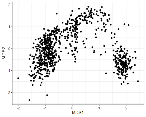
In this article, we propose a graph-aligned random partition model (GARP) that exploits the flexible, but tractable, building blocks of Gibbs-type priors to build a random partition aligned on a graph. The desired interpretation of clusters as vertices and edges in a graph naturally gives rise to dependent priors on cluster-specific parameters. In the motivating example with single-cell RNA-seq data, vertex-clusters represent homogeneous cell subpopulations and edge-clusters correspond to cells that are transitioning between those. See Figure 1 for a scatter plot of single-cell RNA data in a two-dimensional space that captures most of the recorded genetic expressions of mice stem cell data.
Refer to caption
Figure 1: Two-dimensional representation of genetic expressions of the RNA mice single-cells data.

The remainder of the article is as follows. In Section 2 we introduce a model for graph-aligned probabilistic clustering. In Section 3 we introduce special examples. In Sections 4, 5 and 6 we study a useful approximation, implied homogeneity assumptions, and identifiability of vertices versus edges. Section 7 applies the model to single-cell RNA-seq data of mice stem cells and Section 8 concludes with final comments. Substantive additional details, including code, proofs, validations on simulated data, a characterization in terms of discrete probabilities, a discussion of the hyperparameters’ choice, and details on the strategy to obtain point estimates from posterior samples are available as an online supplement.

2 Graph-Aligned Random Partition Model

We introduce a graph-aligned random partition model (GARP) for 𝒚={𝒚i:i=1,,N}𝒚conditional-setsubscript𝒚𝑖𝑖1𝑁\bm{y}=\{\bm{y}_{i}:i=1,\ldots,N\}, 𝒚idsubscript𝒚𝑖superscript𝑑\bm{y}_{i}\in\mathbbm{R}^{d}. The two main features of the model are a two-level random partition structure that assigns observations into vertex-clusters and edge-clusters, and a mixture of normal sampling models with cluster-specific parameters that reflect this split into vertex and edge-clusters. That is, the mixture of normal models is set up such that observations in vertex-clusters form homogeneous subsets in the Euclidean space, and observations in edge-clusters are located between the adjacent vertices. We characterize the model in three different representations that are minor variations of representations that are traditionally used for infinitely exchangeable random partition models (Pitman, 1996), including (1) the probability mass function (pmf) of the graph-aligned random partition via the introduction of exchangeable partition probability functions (EPPF); (2) a composition of Pólya urn schemes, i.e., predictive probability functions, using a generalized CRP (gCRP); and (3) the configuration of ties that is implied by sampling from a composition of discrete random probability measures, similar to the construction of species sampling processes (SSP). See Pitman (1996) and Lee et al. (2013a) for details on these three characterizations for infinitely exchangeable random partitions (without alignment on a graph).

2.1 A Gaussian Mixture over Vertices and Edges

We start the model construction with a sampling model given the latent graph-aligned partition. We need some notation. Let Visubscript𝑉𝑖V_{i} be an indicator for observation i𝑖i being placed into a vertex-cluster and let Zisubscript𝑍𝑖Z_{i} denote a cluster membership indicator. We write 𝑽=(V1,,VN)𝑽subscript𝑉1subscript𝑉𝑁\bm{V}=(V_{1},\ldots,V_{N}) and 𝒁=(Z1,,ZN)𝒁subscript𝑍1subscript𝑍𝑁\bm{Z}=(Z_{1},\ldots,Z_{N}) (throughout 𝒙𝒙\bm{x} denotes the collection of all previously defined elements xasubscript𝑥𝑎x_{a}). We denote with Nv,N=i=1NVisubscript𝑁𝑣𝑁superscriptsubscript𝑖1𝑁subscript𝑉𝑖N_{v,N}=\sum_{i=1}^{N}V_{i} the number of observations in vertex-clusters, and with Ne,N=NNv,Nsubscript𝑁𝑒𝑁𝑁subscript𝑁𝑣𝑁N_{e,N}=N-N_{v,N} the implied number in edge-clusters. For notational simplicity, we drop the subscript N when implied by the context. If i𝑖i belongs to a vertex (i.e., Vi=1subscript𝑉𝑖1V_{i}=1), then Zi[Kv]{1,,Kv}subscript𝑍𝑖delimited-[]subscript𝐾𝑣1subscript𝐾𝑣Z_{i}\in[K_{v}]\equiv\{1,\ldots,K_{v}\}, where Kvsubscript𝐾𝑣K_{v} is the random number of vertex-clusters. If i𝑖i belongs to an edge (i.e., Vi=0subscript𝑉𝑖0V_{i}=0), then Zi=(k,k)subscript𝑍𝑖𝑘superscript𝑘Z_{i}=(k,k^{\prime}), with k<k𝑘superscript𝑘k<k^{\prime} indicating the adjacent vertex-clusters. Let Kesubscript𝐾𝑒K_{e} denote the number of edge-clusters. Clearly, an edge must connect two vertices, implying KeKv(Kv1)2Mesubscript𝐾𝑒subscript𝐾𝑣subscript𝐾𝑣12subscript𝑀𝑒K_{e}\leq\frac{K_{v}(K_{v}-1)}{2}\equiv M_{e}. Finally, let 𝒁𝒗=(Zi:Vi=1)\bm{Z_{v}}=(Z_{i}:V_{i}=1) and 𝒁𝒆=(Zi:Vi=0)\bm{Z_{e}}=(Z_{i}:V_{i}=0) denote the set of cluster membership indicators for vertices and edges, respectively.

Given a graph-aligned random partition, we assume normal sampling

𝒚iZi,𝝁,𝚺indN(𝒚i𝝁Zi,𝚺Zi),(i=1,,N),\bm{y}_{i}\mid Z_{i},\bm{\mu^{\ast}},\bm{\Sigma^{\ast}}\overset{\text{ind}}{\sim}\text{N}(\bm{y}_{i}\mid\bm{\mu^{\ast}}_{Z_{i}},\bm{\Sigma^{\ast}}_{Z_{i}}),\quad(i=1,\ldots,N), (1)

keeping in mind that Zi=ksubscript𝑍𝑖𝑘Z_{i}=k for Vi=1subscript𝑉𝑖1V_{i}=1 and Zi=(k,k)subscript𝑍𝑖𝑘superscript𝑘Z_{i}=(k,k^{\prime}) for Vi=0subscript𝑉𝑖0V_{i}=0. The cluster-specific parameters are defined as follows. For the vertex-parameters 𝜽k=(𝝁k,𝚺k)subscriptsuperscript𝜽bold-∗𝑘subscriptsuperscript𝝁bold-∗𝑘subscriptsuperscript𝚺bold-∗𝑘\bm{\theta^{\ast}}_{k}=(\bm{\mu^{\ast}}_{k},\bm{\Sigma^{\ast}}_{k}) we assume (conditionally) conjugate normal-inverse Wishart priors

𝜽kKviidNIW(𝝁0,λ0,κ0,𝚺0),(k=1,,Kv).conditionalsuperscriptsubscript𝜽𝑘subscript𝐾𝑣iidsimilar-toNIWsubscript𝝁0subscript𝜆0subscript𝜅0subscript𝚺0𝑘1subscript𝐾𝑣\bm{\theta}_{k}^{\ast}\mid K_{v}\overset{\text{iid}}{\sim}\text{NIW}(\bm{\mu}_{0},\lambda_{0},\kappa_{0},\bm{\Sigma}_{0}),\quad(k=1,\ldots,K_{v}). (2)

For edge-clusters, cluster-specific parameters 𝜽k,k=(𝝁k,k,𝚺k,k)subscriptsuperscript𝜽bold-∗𝑘superscript𝑘subscriptsuperscript𝝁bold-∗𝑘superscript𝑘subscriptsuperscript𝚺bold-∗𝑘superscript𝑘\bm{\theta^{\ast}}_{k,k^{\prime}}=(\bm{\mu^{\ast}}_{k,k^{\prime}},\bm{\Sigma^{\ast}}_{k,k^{\prime}}) are defined as functions of the adjacent vertex-clusters,

𝝁k,k=𝝁k+𝝁k2,𝚺k,k=f(𝝁k,𝝁k,r0,r1).formulae-sequencesubscriptsuperscript𝝁bold-∗𝑘superscript𝑘subscriptsuperscript𝝁bold-∗𝑘subscriptsuperscript𝝁bold-∗superscript𝑘2subscriptsuperscript𝚺bold-∗𝑘superscript𝑘𝑓subscriptsuperscript𝝁bold-∗𝑘subscriptsuperscript𝝁bold-∗superscript𝑘subscript𝑟0subscript𝑟1\bm{\mu^{\ast}}_{k,k^{\prime}}=\frac{\bm{\mu^{\ast}}_{k}+\bm{\mu^{\ast}}_{k^{\prime}}}{2},~{}~{}\bm{\Sigma^{\ast}}_{k,k^{\prime}}=f(\bm{\mu^{\ast}}_{k},\bm{\mu^{\ast}}_{k^{\prime}},r_{0},r_{1}). (3)

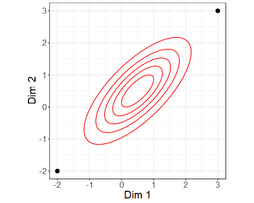
Here f𝑓f is such that the α%percent𝛼\alpha\%-level contour of the N(𝝁k,k,𝚺k,k)𝑁subscriptsuperscript𝝁bold-∗𝑘superscript𝑘subscriptsuperscript𝚺bold-∗𝑘superscript𝑘N(\bm{\mu^{\ast}}_{k,k^{\prime}},\bm{\Sigma^{\ast}}_{k,k^{\prime}}) density is stretched around the line Lk,ksubscript𝐿𝑘superscript𝑘L_{k,k^{\prime}} connecting 𝝁ksubscriptsuperscript𝝁bold-∗𝑘\bm{\mu^{\ast}}_{k} and 𝝁ksubscriptsuperscript𝝁bold-∗superscript𝑘\bm{\mu^{\ast}}_{k^{\prime}}, the Gaussian component projected onto Lk,ksubscript𝐿𝑘superscript𝑘L_{k,k^{\prime}} has standard deviation r0𝝁k𝝁ksubscript𝑟0normsubscriptsuperscript𝝁bold-∗𝑘superscriptsubscript𝝁superscript𝑘r_{0}\,||\bm{\mu^{\ast}}_{k}-\bm{\mu}_{k^{\prime}}^{\ast}||, and the projection onto the orthogonal complement Lk,ksuperscriptsubscript𝐿𝑘superscript𝑘perpendicular-toL_{k,k^{\prime}}^{\perp} are d1𝑑1d-1 independent Gaussian distributions with variances r12superscriptsubscript𝑟12r_{1}^{2}. Figure S.1 in Section S.1 of the supplemental materials shows the contour plot of an edge-cluster in 2superscript2\mathbbm{R}^{2}. See the same section and Section S.3 of the supplementary materials for more discussion of 𝚺k,ksubscriptsuperscript𝚺bold-∗𝑘superscript𝑘\bm{\Sigma^{\ast}}_{k,k^{\prime}}, and comments on the choice of hyperparameters r0,r1subscript𝑟0subscript𝑟1r_{0},r_{1}.

2.2 Graph-Aligned Random Partition (GARP)

We introduce a flexible graph-aligned random partition model. In words, we first label each item as belonging to a vertex or edge cluster (with probability pvsubscript𝑝𝑣p_{v} and (1pv)1subscript𝑝𝑣(1-p_{v}), respectively), then use a Gibbs-type prior to cluster items associated with vertices, and a Dirichlet-multinomial prior to place those associated with edges into one of the Mesubscript𝑀𝑒M_{e} possible edges, respectively. Let (n1,,nKv)subscript𝑛1subscript𝑛subscript𝐾𝑣(n_{1},\ldots,n_{K_{v}}) denote the cardinalities of the vertex-clusters, i.e., nk=i𝟙({Vi=1}{Zi=k})subscript𝑛𝑘subscript𝑖1subscript𝑉𝑖1subscript𝑍𝑖𝑘n_{k}=\sum_{i}\mathbbm{1}(\{V_{i}=1\}\cap\{Z_{i}=k\}), and similarly let nk,k=i𝟙({Vi=0}{Zi=(k,k)})subscript𝑛𝑘superscript𝑘subscript𝑖1subscript𝑉𝑖0subscript𝑍𝑖𝑘superscript𝑘n_{k,k^{\prime}}=\sum_{i}\mathbbm{1}(\{V_{i}=0\}\cap\{Z_{i}=(k,k^{\prime})\}) denote the sizes of the implied edge-clusters, with nk,k=0subscript𝑛𝑘superscript𝑘0n_{k,k^{\prime}}=0 indicating the lack of an edge between k,k𝑘superscript𝑘k,k^{\prime}. We define a graph-aligned random partition model via the pmf of 𝑽,𝒁𝑽𝒁\bm{V},\bm{Z}

G(N)(𝑽,𝒁)pvNvEPPFKv(Nv)(n1,,nKvα,σ)/Kv!(1pv)NeDMMe(Ne)((nk,k)k<kβ/Me) 1({Ne=0}{Me>0}EN),proportional-tosuperscript𝐺𝑁𝑽𝒁superscriptsubscript𝑝𝑣subscript𝑁𝑣superscriptsubscriptEPPFsubscript𝐾𝑣subscript𝑁𝑣subscript𝑛1conditionalsubscript𝑛subscript𝐾𝑣𝛼𝜎subscript𝐾𝑣superscript1subscript𝑝𝑣subscript𝑁𝑒superscriptsubscriptDMsubscript𝑀𝑒subscript𝑁𝑒conditionalsubscriptsubscript𝑛𝑘superscript𝑘𝑘superscript𝑘𝛽subscript𝑀𝑒1subscriptsubscript𝑁𝑒0subscript𝑀𝑒0subscript𝐸𝑁\displaystyle\begin{split}G^{(N)}(\bm{V},\bm{Z})&\propto p_{v}^{N_{v}}\,\mathrm{EPPF}_{K_{v}}^{(N_{v})}(n_{1},\ldots,n_{K_{v}}\mid\alpha,\sigma)/K_{v}!\\ &(1-p_{v})^{N_{e}}\text{DM}_{M_{e}}^{(N_{e})}((n_{k,k^{\prime}})_{k<k^{\prime}}\mid\beta/M_{e})\,\mathbbm{1}(\underbrace{\{N_{e}=0\}\cup\{M_{e}>0\}}_{E_{N}}),\end{split} (4)

where EPPF(α,σ)\mathrm{EPPF}(\cdot\mid\alpha,\sigma) denotes the EPPF of a Gibbs-type prior, DM is the marginal likelihood of an Mesubscript𝑀𝑒M_{e}-symmetric Dirichlet-multinomial model (for categorical realizations, and defining DM(0)()=DM0()()1superscriptsubscriptDM0superscriptsubscriptDM01\text{DM}_{\cdot}^{(0)}(\cdot)=\text{DM}_{0}^{(\cdot)}(\cdot)\equiv 1) and 𝟙({Ne=0}{Me>0})1subscript𝑁𝑒0subscript𝑀𝑒0\mathbbm{1}(\{N_{e}=0\}\cup\{M_{e}>0\}) is an indicator that represents the constraint that edges can only be assigned if there are at least 2 vertices (Me>0subscript𝑀𝑒0M_{e}>0, that is, Kv>1subscript𝐾𝑣1K_{v}>1), or no units are assigned to edges (Ne=0subscript𝑁𝑒0N_{e}=0). We will use ENsubscript𝐸𝑁E_{N} to refer to this truncation event. In particular, when Kv=1subscript𝐾𝑣1K_{v}=1 (and therefore Me=0subscript𝑀𝑒0M_{e}=0) (4) reduces to G(N)(𝑽,𝒁)pvNEPPF1(N)(Nα,σ)proportional-tosuperscript𝐺𝑁𝑽𝒁superscriptsubscript𝑝𝑣𝑁superscriptsubscriptEPPF1𝑁conditional𝑁𝛼𝜎G^{(N)}(\bm{V},\bm{Z})\propto p_{v}^{N}\,\mathrm{EPPF}_{1}^{(N)}(N\mid\alpha,\sigma) with Vi=Zi=1subscript𝑉𝑖subscript𝑍𝑖1V_{i}=Z_{i}=1, for all i𝑖i, and G(N)(𝑽,𝒁)=0superscript𝐺𝑁𝑽𝒁0G^{(N)}(\bm{V},\bm{Z})=0 for any other configuration (𝑽,𝒁)𝑽𝒁(\bm{V},\bm{Z}), e.g., any configuration with Ne>0subscript𝑁𝑒0N_{e}>0 (i.e., ENcsuperscriptsubscript𝐸𝑁𝑐E_{N}^{c}).

An EPPF characterizes the distribution of an exchangeable partition (Pitman, 1996), with EPPFKv(Nv)(n1,,nKv)superscriptsubscriptEPPFsubscript𝐾𝑣subscript𝑁𝑣subscript𝑛1subscript𝑛subscript𝐾𝑣\mathrm{EPPF}_{K_{v}}^{(N_{v})}(n_{1},\ldots,n_{K_{v}}) being the probability of observing a particular (unordered) partition of Nvsubscript𝑁𝑣N_{v} observations into Kvsubscript𝐾𝑣K_{v} subsets of cardinalities {n1,,nKv}subscript𝑛1subscript𝑛subscript𝐾𝑣\{n_{1},\ldots,n_{K_{v}}\}. Since an EPPF refers to unordered partitions we include the additional denominator Kv!subscript𝐾𝑣K_{v}! for the ordered 𝒁𝒁\bm{Z}. See Section 4 for more discussions of the homogeneity assumptions implied by our model. We specify the EPPF as a Gibbs-type prior,

EPPFKv(Nv)(n1,,nKvα,σ)=WNv,Kvk=1Kv(1σ)nk1,superscriptsubscriptEPPFsubscript𝐾𝑣subscript𝑁𝑣subscript𝑛1conditionalsubscript𝑛subscript𝐾𝑣𝛼𝜎subscript𝑊subscript𝑁𝑣subscript𝐾𝑣superscriptsubscriptproduct𝑘1subscript𝐾𝑣subscript1𝜎subscript𝑛𝑘1\displaystyle\mathrm{EPPF}_{K_{v}}^{(N_{v})}(n_{1},\ldots,n_{K_{v}}\mid\alpha,\sigma)=W_{N_{v},K_{v}}\prod_{k=1}^{K_{v}}(1-\sigma)_{n_{k}-1}, (5)

where (x)n=x(x+1)(x+n1)subscript𝑥𝑛𝑥𝑥1𝑥𝑛1(x)_{n}=x(x+1)\ldots(x+n-1) represents the ascending factorial, σ<1𝜎1\sigma<1 is a discount parameter and the set of non-negative weights {Wn,k:1kn}conditional-setsubscript𝑊𝑛𝑘1𝑘𝑛\{W_{n,k}:1\leq k\leq n\} satisfies the recursive equation Wn,k=(nσk)Wn+1,k+Wn+1,k+1subscript𝑊𝑛𝑘𝑛𝜎𝑘subscript𝑊𝑛1𝑘subscript𝑊𝑛1𝑘1W_{n,k}=(n-\sigma k)W_{n+1,k}+W_{n+1,k+1}. The parameter α𝛼\alpha in the conditioning set is used to define Wn,ksubscript𝑊𝑛𝑘W_{n,k} for some of the upcoming examples. In a second step, the observations assigned to edges are (ordered) clustered using a DM distribution.

G(N)((Zi:Vi=0)𝑽,Kv)=DMMe(Ne)((nk,k)k<kvβ/Me)==Γ(β)Γ(Ne+β/Me)(k,k):k<kKvΓ(nk,k+β/Me)Γ(β/Me).G^{(N)}((Z_{i}:~{}V_{i}=0)\mid\bm{V},K_{v})=\text{DM}_{M_{e}}^{(N_{e})}((n_{k,k^{\prime}})_{k<k_{v}^{\prime}}\mid\beta/M_{e})=\\ =\frac{\Gamma(\beta)}{\Gamma(N_{e}+\beta/M_{e})}\prod_{(k,k^{\prime}):k<k^{\prime}\leq K_{v}}\frac{\Gamma(n_{k,k^{\prime}}+\beta/M_{e})}{\Gamma(\beta/M_{e})}. (6)

Model (4) is a hierarchical constrained composition of a Gibbs-type prior and a symmetric-DM with hyperparameter β/Me𝛽subscript𝑀𝑒\beta/M_{e}. As we shall show, the model preserves most of the analytical and computational tractability of the simpler building blocks.

2.3 Generalized Chinese Restaurant Process

In an alternative characterization of (4), the model can be defined as a truncated version of a composition of gCRP. We denote the latter, that is, the model before the truncation, as G(N)~~superscript𝐺𝑁\widetilde{G^{(N)}} and refer to it as the relaxed model.

G(N)(𝑽,𝒁)G(N)~(𝑽,𝒁)𝟙(EN).proportional-tosuperscript𝐺𝑁𝑽𝒁~superscript𝐺𝑁𝑽𝒁1subscript𝐸𝑁G^{(N)}(\bm{V},\bm{Z})\propto\widetilde{G^{(N)}}(\bm{V},\bm{Z})\mathbbm{1}(E_{N}). (7)

Recall that EN={Ne=0}{Me>0}subscript𝐸𝑁subscript𝑁𝑒0subscript𝑀𝑒0E_{N}=\{N_{e}=0\}\cup\{M_{e}>0\} is the truncation. In Section 4 we show that G(N)~~superscript𝐺𝑁\widetilde{G^{(N)}} assigns high probability to ENsubscript𝐸𝑁E_{N}, going to 111 with n𝑛n\to\infty for most Gibbs-type priors.

The relaxed model G(N)~(𝑽,𝒁)~superscript𝐺𝑁𝑽𝒁\widetilde{G^{(N)}}(\bm{V},\bm{Z}) is a hierarchical composition of tractable generalized Pólya urn schemes, starting with the assignments to vertices or edges

ViiidBern(pv),(i=1,,N).subscript𝑉𝑖iidsimilar-toBernsubscript𝑝𝑣𝑖1𝑁V_{i}\overset{\text{iid}}{\sim}\text{Bern}(p_{v}),\quad(i=1,\ldots,N). (8)

Next, we sample cluster membership indicators 𝒁𝒗=(Zi:Vi=1)\bm{Z_{v}}=(Z_{i}:\;V_{i}=1) for the vertex-clusters from the gCRP associated with Gibbs-type prior, i.e., 𝒁𝒗𝑽gCRP(α,σ)similar-toconditionalsubscript𝒁𝒗𝑽gCRP𝛼𝜎\bm{Z_{v}}\mid\bm{V}\sim\text{gCRP}(\alpha,\sigma), with the gCRP implied by G(N)~~superscript𝐺𝑁\widetilde{G^{(N)}} given as

G(N)~{Zi=k𝒁i,𝑽i,Vi=1}={WNv,KviWNv1,Kvik=1Kvi(nkiσ)k[Kvi]WNv,Kvi+1WNv1,Kvik=Kvi+1.~superscript𝐺𝑁conditional-setsubscript𝑍𝑖𝑘superscript𝒁𝑖superscript𝑽𝑖subscript𝑉𝑖1casessubscript𝑊subscript𝑁𝑣superscriptsubscript𝐾𝑣𝑖subscript𝑊subscript𝑁𝑣1superscriptsubscript𝐾𝑣𝑖superscriptsubscript𝑘1superscriptsubscript𝐾𝑣𝑖superscriptsubscript𝑛𝑘𝑖𝜎𝑘delimited-[]superscriptsubscript𝐾𝑣𝑖subscript𝑊subscript𝑁𝑣superscriptsubscript𝐾𝑣𝑖1subscript𝑊subscript𝑁𝑣1superscriptsubscript𝐾𝑣𝑖𝑘superscriptsubscript𝐾𝑣𝑖1\widetilde{G^{(N)}}\{Z_{i}=k\mid\bm{Z}^{-i},\bm{V}^{-i},V_{i}=1\}=\begin{cases}\frac{W_{N_{v},K_{v}^{-i}}}{W_{N_{v}-1,K_{v}^{-i}}}\sum_{k=1}^{K_{v}^{-i}}(n_{k}^{-i}-\sigma)&k\in[K_{v}^{-i}]\vspace*{0.2cm}\\ \frac{W_{N_{v},K_{v}^{-i}+1}}{W_{N_{v}-1,K_{v}^{-i}}}&k=K_{v}^{-i}+1.\end{cases} (9)

Throughout 𝐱isuperscript𝐱𝑖\mathbf{x}^{-i} identifies a quantity after removing the element i𝑖i from 𝐱𝐱\mathbf{x}. See Section 3 for examples of different gCRP and implied prior assumptions on the number of vertices.

Finally, the cluster membership indicators 𝒁𝒆subscript𝒁𝒆\bm{Z_{e}} for the observations in edges follow the Pólya urn scheme induced by a DM distribution

G(N)~{Zi=(k,k)Vi=0,𝒁i,EN}nk,ki+β/Me,proportional-to~superscript𝐺𝑁conditional-setsubscript𝑍𝑖𝑘superscript𝑘subscript𝑉𝑖0superscript𝒁𝑖subscript𝐸𝑁superscriptsubscript𝑛𝑘superscript𝑘𝑖𝛽subscript𝑀𝑒\widetilde{G^{(N)}}\{Z_{i}=(k,k^{\prime})\mid V_{i}=0,\bm{Z}^{-i},E_{N}\}\propto n_{k,k^{\prime}}^{-i}+\beta/M_{e}, (10)

with k<kKvsuperscript𝑘𝑘subscript𝐾𝑣k^{\prime}<k\leq K_{v}. Here, β/Me𝛽subscript𝑀𝑒\beta/M_{e} favors sparsity as the dimension of the graph increases. Note that (8) might generate Ne>0subscript𝑁𝑒0N_{e}>0, even when (9) implies Me=0subscript𝑀𝑒0M_{e}=0. For this case we define for completeness G(N)~{Zi=(1,2)Vi=0,𝒁i,ENc}1~superscript𝐺𝑁conditional-setsubscript𝑍𝑖12subscript𝑉𝑖0superscript𝒁𝑖superscriptsubscript𝐸𝑁𝑐1\widetilde{G^{(N)}}\{Z_{i}=(1,2)\mid V_{i}=0,\bm{Z}^{-i},E_{N}^{c}\}\equiv 1 (without implications for G(N)superscript𝐺𝑁G^{(N)}, due to the truncation to ENsubscript𝐸𝑁E_{N} in (7)).

The aforementioned composition of urn schemes characterizes the GARP (4):

Proposition 1.

The random partition structure of the GARP model (4) can be characterized as the truncated composition of gCRP defined in (7), (8), (9) and (10).

We rely on this representation to derive an MCMC algorithm that generalizes the marginal MCMC algorithms for DP mixture models and Gibbs-type priors (Neal, 2000; De Blasi et al., 2015; Miller and Harrison, 2018). Moreover, as we shall see, the probability of the truncation event ENsubscript𝐸𝑁E_{N} is high and rapidly goes to 111 in most cases.

Composition of Discrete Random Probabilities.

Finally, in Section S.2 of the supplementary materials we derive a third characterization of the proposed GARP. We define G(N)~~superscript𝐺𝑁\widetilde{G^{(N)}} as a graph-aligned random partition (with unique atoms) implied by the ties under conditionally i.i.d. sampling of 𝜽isubscript𝜽𝑖\bm{\theta}_{i}. Such a characterization will be used in a lemma to prove Theorem 3 and can be used to connect with existing BNP literature to derive a conditional Gibbs sampler.

3 Specific Model Choices

Conditioning on the vertex assignments 𝑽𝑽\bm{V}, under the relaxed model G(N)~~superscript𝐺𝑁\widetilde{G^{(N)}} the distribution of the clustering indicators 𝒁vsubscript𝒁𝑣\bm{Z}_{v} is given by the EPPF of a Gibbs-type prior (Gnedin and Pitman, 2006; De Blasi et al., 2015). We introduce four specific choices, stating the EPPFKv(Nv)(n1,,nKv)superscriptsubscriptEPPFsubscript𝐾𝑣subscript𝑁𝑣subscript𝑛1subscript𝑛subscript𝐾𝑣\mathrm{EPPF}_{K_{v}}^{(N_{v})}(n_{1},\ldots,n_{K_{v}}) for partitioning Nvsubscript𝑁𝑣N_{v} observations into Kvsubscript𝐾𝑣K_{v} vertices. Table 1 shows the corresponding expressions for G(N)~{Zi=kVi=1,𝒁vi,𝑽i}~superscript𝐺𝑁conditional-setsubscript𝑍𝑖𝑘subscript𝑉𝑖1superscriptsubscript𝒁𝑣𝑖superscript𝑽𝑖\widetilde{G^{(N)}}\{Z_{i}=k\mid V_{i}=1,\bm{Z}_{v}^{-i},\bm{V}^{-i}\} in the gCRP of (9), and the weights and atoms for Pv=m=1Mvπmδ𝜽~msubscript𝑃𝑣superscriptsubscript𝑚1subscript𝑀𝑣subscript𝜋𝑚subscript𝛿subscript~𝜽𝑚P_{v}=\sum_{m=1}^{M_{v}}\pi_{m}\delta_{\tilde{\bm{\theta}}_{m}} in (S.1). Throughout, the prior for cluster-specific parameters remains the NIW in (2).

Table 1: G(N)~{Zi=k}~superscript𝐺𝑁conditional-setsubscript𝑍𝑖𝑘\widetilde{G^{(N)}}\{Z_{i}=k\mid\ldots\} in the gCRP (9), and weights (πm)m+1Mvsuperscriptsubscriptsubscript𝜋𝑚𝑚1subscript𝑀𝑣(\pi_{m})_{m+1}^{M_{v}} for Pv=m=1Mvπmδ𝜽~msubscript𝑃𝑣superscriptsubscript𝑚1subscript𝑀𝑣subscript𝜋𝑚subscript𝛿subscript~𝜽𝑚P_{v}=\sum_{m=1}^{M_{v}}\pi_{m}\delta_{\tilde{\bm{\theta}}_{m}} in (S.1).
        G(N)~{Zi=kVi=1,𝒁vi,𝑽i}proportional-to~superscript𝐺𝑁conditional-setsubscript𝑍𝑖𝑘subscript𝑉𝑖1superscriptsubscript𝒁𝑣𝑖superscript𝑽𝑖absent\widetilde{G^{(N)}}\{Z_{i}=k\mid V_{i}=1,\bm{Z}_{v}^{-i},\bm{V}^{-i}\}\propto P(π1,π2,Mv)𝑃subscript𝜋1subscript𝜋2conditionalsubscript𝑀𝑣P(\pi_{1},\pi_{2},\ldots\mid M_{v}) p(Mv=m)𝑝subscript𝑀𝑣𝑚p(M_{v}=m)
Ex. k𝒁vi𝑘superscriptsubscript𝒁𝑣𝑖k\in\bm{Z}_{v}^{-i} k=Kvi+1𝑘superscriptsubscript𝐾𝑣𝑖1k=K_{v}^{-i}+1
1 nki+ρsuperscriptsubscript𝑛𝑘𝑖𝜌n_{k}^{-i}+\rho ρ(MvKvi)(a)𝜌superscriptsubscript𝑀𝑣superscriptsubscript𝐾𝑣𝑖𝑎\rho(M_{v}-K_{v}^{-i})\;^{(a)} Dir(ρ,,ρ)Dir𝜌𝜌\text{Dir}(\rho,\ldots,\rho) fixed Mvsubscript𝑀𝑣M_{v}\in\mathbb{N}
2 (nki+1)×(n_{k}^{-i}+1)\;\times (Kvi)2Kviγsuperscriptsuperscriptsubscript𝐾𝑣𝑖2superscriptsubscript𝐾𝑣𝑖𝛾(K_{v}^{-i})^{2}-K_{v}^{-i}\gamma Dir(1,,1)Dir11\text{Dir}(1,\ldots,1) γ(1γ)m1m!𝛾subscript1𝛾𝑚1𝑚\frac{\gamma(1-\gamma)_{m-1}}{m!}
(NviKvi+γ)superscriptsubscript𝑁𝑣𝑖superscriptsubscript𝐾𝑣𝑖𝛾~{}~{}(N_{v}^{-i}-K_{v}^{-i}+\gamma)
3 nkisuperscriptsubscript𝑛𝑘𝑖n_{k}^{-i} α𝛼\alpha GEM(α)(b)GEMsuperscript𝛼𝑏\text{GEM}(\alpha)\;^{(b)} Mv=subscript𝑀𝑣M_{v}=\infty
4 nkiσsuperscriptsubscript𝑛𝑘𝑖𝜎n_{k}^{-i}-\sigma α+Kviσ𝛼superscriptsubscript𝐾𝑣𝑖𝜎\alpha+K_{v}^{-i}\sigma GEM(α,σ)(b)GEMsuperscript𝛼𝜎𝑏\text{GEM}(\alpha,\sigma)\;^{(b)} Mv=subscript𝑀𝑣M_{v}=\infty

(a) subject to Kvi<Mvsuperscriptsubscript𝐾𝑣𝑖subscript𝑀𝑣K_{v}^{-i}<M_{v}.
(b) GEM stands for the distribution of probability weights after Griffiths, Engen, and McCloskey (Ewens, 1990), using the 1-parameter version defined there and the related 2-parameters extension.

Example 1 (Mvsubscript𝑀𝑣M_{v}-dimensional symmetric Dirichlet).

If prior information on an upper bound Mvsubscript𝑀𝑣M_{v} on the number of vertices is available we can proceed with a finite-dimensional symmetric Dirichlet prior (Green and Richardson, 2001).

EPPFKv(Nv)(n1,,nKv)=Mv!(MvKv)!Γ(ρMv)Γ(Nv+ρMv)Γ(ρ)Kvk=1KvΓ(nk+ρ).superscriptsubscriptEPPFsubscript𝐾𝑣subscript𝑁𝑣subscript𝑛1subscript𝑛subscript𝐾𝑣subscript𝑀𝑣subscript𝑀𝑣subscript𝐾𝑣Γ𝜌subscript𝑀𝑣Γsubscript𝑁𝑣𝜌subscript𝑀𝑣Γsuperscript𝜌subscript𝐾𝑣superscriptsubscriptproduct𝑘1subscript𝐾𝑣Γsubscript𝑛𝑘𝜌\mathrm{EPPF}_{K_{v}}^{(N_{v})}(n_{1},\ldots,n_{K_{v}})=\frac{M_{v}!}{(M_{v}-K_{v})!}\frac{\Gamma(\rho\,M_{v})}{\Gamma(N_{v}+\rho\,M_{v})\Gamma(\rho)^{K_{v}}}\prod_{k=1}^{K_{v}}\Gamma(n_{k}+\rho). (11)

Allowing for unknown Mvsubscript𝑀𝑣M_{v} the model becomes a mixture of symmetric Dirichlet, that is, a mixture of finite mixtures (MFM). MFMs can be particularly interesting for allowing consistent estimation of any finite number of clusters (Nobile, 1994; Miller and Harrison, 2018). MFMs are a special case of Gibbs-type priors. A relevant example is the Gnedin process.

Example 2 (Gnedin process, with σ=1𝜎1\sigma=-1).

Under the Gnedin prior with parameter γ(0,1)𝛾01\gamma\in(0,1) the EPPFKv(Nv)superscriptsubscriptEPPFsubscript𝐾𝑣subscript𝑁𝑣\mathrm{EPPF}_{K_{v}}^{(N_{v})} in (4) becomes

EPPFKv(Nv)(n1,,nKv)=m=1EPPFKv(Nv)(n1,,nKvMv=m)p(Mv=m),superscriptsubscriptEPPFsubscript𝐾𝑣subscript𝑁𝑣subscript𝑛1subscript𝑛subscript𝐾𝑣superscriptsubscript𝑚1superscriptsubscriptEPPFsubscript𝐾𝑣subscript𝑁𝑣subscript𝑛1conditionalsubscript𝑛subscript𝐾𝑣subscript𝑀𝑣𝑚𝑝subscript𝑀𝑣𝑚\mathrm{EPPF}_{K_{v}}^{(N_{v})}(n_{1},\ldots,n_{K_{v}})=\sum_{m=1}^{\infty}\mathrm{EPPF}_{K_{v}}^{(N_{v})}(n_{1},\ldots,n_{K_{v}}\mid M_{v}=m)\,p(M_{v}=m),

where EPPFKv(Nv)(n1,,nKvMv=m)superscriptsubscriptEPPFsubscript𝐾𝑣subscript𝑁𝑣subscript𝑛1conditionalsubscript𝑛subscript𝐾𝑣subscript𝑀𝑣𝑚\mathrm{EPPF}_{K_{v}}^{(N_{v})}(n_{1},\ldots,n_{K_{v}}\mid M_{v}=m) is the EPPF of the Mvsubscript𝑀𝑣M_{v}-symmetric Dirichlet prior in (11), with ρ=1𝜌1\rho=1 and p(Mv=m)=γ(1γ)m1m!.𝑝subscript𝑀𝑣𝑚𝛾subscript1𝛾𝑚1𝑚p(M_{v}=m)=\frac{\gamma(1-\gamma)_{m-1}}{m!}.

The gCRP for the Gnedin process allows tractable analytical results and efficient algorithms. Moreover, the Gnedin process entails a distribution on the number of components Mvsubscript𝑀𝑣M_{v} that has the mode at 111, a heavy tail, and infinite expectation (Gnedin, 2010). Therefore, the implied MFM favors a small number of vertices, while also being robust due to the heavy tail distribution of Mvsubscript𝑀𝑣M_{v}.

Note that one can use Mv=subscript𝑀𝑣M_{v}=\infty to let the number of vertices (i.e., Kvsubscript𝐾𝑣K_{v}) grow to infinity with Nvsubscript𝑁𝑣N_{v}. Examples are the DP which entails a logarithmic growth of the number of vertices and the PYP which entails a polynomial growth of the number of vertices.

Example 3 (DP).

Under the DP prior with parameter α>0𝛼0\alpha>0 the EPPFKv(Nv)superscriptsubscriptEPPFsubscript𝐾𝑣subscript𝑁𝑣\mathrm{EPPF}_{K_{v}}^{(N_{v})} in (4) becomes

EPPFKv(Nv)(n1,,nKv)=αKvΓ(α)Γ(α+Nv)k=1Kv(nk1)!superscriptsubscriptEPPFsubscript𝐾𝑣subscript𝑁𝑣subscript𝑛1subscript𝑛subscript𝐾𝑣superscript𝛼subscript𝐾𝑣Γ𝛼Γ𝛼subscript𝑁𝑣superscriptsubscriptproduct𝑘1subscript𝐾𝑣subscript𝑛𝑘1\mathrm{EPPF}_{K_{v}}^{(N_{v})}(n_{1},\ldots,n_{K_{v}})=\frac{\alpha^{K_{v}}\Gamma(\alpha)}{\Gamma(\alpha+N_{v})}\prod_{k=1}^{K_{v}}(n_{k}-1)!
Example 4 (PYP).

Under a PYP prior with parameters σ[0,1)𝜎01\sigma\in[0,1) and α>0𝛼0\alpha>0 the EPPFKv(Nv)superscriptsubscriptEPPFsubscript𝐾𝑣subscript𝑁𝑣\mathrm{EPPF}_{K_{v}}^{(N_{v})} in (4) becomes

EPPFKv(Nv)(n1,,nKv)=Γ(α+1)k=1Kv1(α+kσ)Γ(α+Nv)k=1Kv(1σ)nk1.superscriptsubscriptEPPFsubscript𝐾𝑣subscript𝑁𝑣subscript𝑛1subscript𝑛subscript𝐾𝑣Γ𝛼1superscriptsubscriptproduct𝑘1subscript𝐾𝑣1𝛼𝑘𝜎Γ𝛼subscript𝑁𝑣superscriptsubscriptproduct𝑘1subscript𝐾𝑣subscript1𝜎subscript𝑛𝑘1\mathrm{EPPF}_{K_{v}}^{(N_{v})}(n_{1},\ldots,n_{K_{v}})=\frac{\Gamma(\alpha+1)\prod_{k=1}^{K_{v}-1}(\alpha+k\sigma)}{\Gamma(\alpha+N_{v})}\prod_{k=1}^{K_{v}}(1-\sigma)_{n_{k}-1}.

With σ=0𝜎0\sigma=0 the PYP reduces to the DP.

With σ=0𝜎0\sigma=0 the PYP reduces to the DP. Other popular sub-classes of Gibbs-type priors include the NGPP (Lijoi et al., 2007b), the NIG (Lijoi et al., 2005, 2007a), and the MFM (Nobile and Fearnside, 2007; Miller and Harrison, 2018). See De Blasi et al. (2015) for a comprehensive review of Gibbs-type priors.

Finally, we note that here we focus on prior elicitation of the Gibbs-type random partition that controls the vertex-clusters and the number of vertices (i.e., Kvmin(Mv,Nv)min(Mv,N)subscript𝐾𝑣subscript𝑀𝑣subscript𝑁𝑣subscript𝑀𝑣𝑁K_{v}\leq\min(M_{v},N_{v})\leq\min(M_{v},N)). Given Kvsubscript𝐾𝑣K_{v} the possible number of edges is finite. The only Gibbs-type prior with a finite fixed number of components Mesubscript𝑀𝑒M_{e} is the symmetric Dirichlet (see e.g, De Blasi et al., 2015), that is the DMMe𝐷subscript𝑀subscript𝑀𝑒DM_{M_{e}} in (4). Although the preceding discussion focuses on the Gibbs-type partition that controls the vertices assignment, it entails (thanks to the hierarchical definition e.g., in Section 2.3) similar flexibility in the joint prior elicitation of the vertices assignments.

4 Goodness of the Approximation

We discuss the nature of the approximation of the GARP model in (4) by the relaxed model G(N)~~superscript𝐺𝑁\widetilde{G^{(N)}}, and why it is a good approximation of G(N)superscript𝐺𝑁G^{(N)}, justifying the prior elicitation of G(N)superscript𝐺𝑁G^{(N)} via G(N)~~superscript𝐺𝑁\widetilde{G^{(N)}}. Importantly, the results allow us to effectively sample from the GARP via rejection sampling, using proposals from G(N)~~superscript𝐺𝑁\widetilde{G^{(N)}}.

Proposition 2.

The probability of the truncation event ENsubscript𝐸𝑁E_{N} in (7) is

G(N)~{EN}=pvN+nv=2N1(Nnv)pvnv(1pv)(Nnv)[1(1σ)nv1Wnv,1].~superscript𝐺𝑁subscript𝐸𝑁superscriptsubscript𝑝𝑣𝑁superscriptsubscriptsubscript𝑛𝑣2𝑁1binomial𝑁subscript𝑛𝑣superscriptsubscript𝑝𝑣subscript𝑛𝑣superscript1subscript𝑝𝑣𝑁subscript𝑛𝑣delimited-[]1subscript1𝜎subscript𝑛𝑣1subscript𝑊subscript𝑛𝑣1\widetilde{G^{(N)}}\{E_{N}\}=p_{v}^{N}+\sum_{n_{v}=2}^{N-1}\binom{N}{n_{v}}p_{v}^{n_{v}}(1-p_{v})^{(N-n_{v})}\big{[}1-(1-\sigma)_{n_{v}-1}W_{n_{v},1}\big{]}. (12)

Here pvN=G(N)~{Nv=N}superscriptsubscript𝑝𝑣𝑁~superscript𝐺𝑁subscript𝑁𝑣𝑁p_{v}^{N}=\widetilde{G^{(N)}}\{N_{v}=N\}, and (1σ)nv1Wnv,1subscript1𝜎subscript𝑛𝑣1subscript𝑊subscript𝑛𝑣1(1-\sigma)_{n_{v}-1}W_{n_{v},1} in the second term arises from (5) as the probability given {Nv=nv}subscript𝑁𝑣subscript𝑛𝑣\{N_{v}=n_{v}\} of having a single vertex, i.e., G(N)~{Kv=1Nv=nv}=EPPF1(nv)(nv)~superscript𝐺𝑁conditional-setsubscript𝐾𝑣1subscript𝑁𝑣subscript𝑛𝑣superscriptsubscriptEPPF1subscript𝑛𝑣subscript𝑛𝑣\widetilde{G^{(N)}}\{K_{v}=1\mid N_{v}=n_{v}\}=\mathrm{EPPF}_{1}^{(n_{v})}(n_{v}). For the Gibbs-type priors in the following examples, the latter reduces to simple analytical expressions.

In the upcoming discussion, we introduce several closely related distributions. To avoid confusion we provide a brief summary and list of defined distributions in Table S.1 in the supplementary materials. Let GVZ(N)~~superscriptsubscript𝐺VZ𝑁\widetilde{G_{\mbox{\tiny VZ}}^{(N)}} denote the law of Visubscript𝑉𝑖V_{i}, i=1,,N𝑖1𝑁i=1,\ldots,N and 𝒁𝒗=(Zi:i[N],Vi=1)\bm{Z_{v}}=(Z_{i}:\;i\in[N],V_{i}=1) under the relaxed model. More precisely, GVZ(N)~~superscriptsubscript𝐺VZ𝑁\widetilde{G_{\mbox{\tiny VZ}}^{(N)}} is the joint law of the random variables (T1,,TN)subscript𝑇1subscript𝑇𝑁(T_{1},\ldots,T_{N}), where Ti=Visubscript𝑇𝑖subscript𝑉𝑖T_{i}=V_{i} if Vi=0subscript𝑉𝑖0V_{i}=0 and Ti=(Vi,Zi)subscript𝑇𝑖subscript𝑉𝑖subscript𝑍𝑖T_{i}=(V_{i},Z_{i}) if Vi=1subscript𝑉𝑖1V_{i}=1. Let GVZ~~subscript𝐺VZ\widetilde{G_{\mbox{\tiny VZ}}} denote the law of the stochastic process with Kolmogorov consistent finite dimensional (GVZ(N)~)Nsubscript~superscriptsubscript𝐺VZ𝑁𝑁(\widetilde{G_{\mbox{\tiny VZ}}^{(N)}})_{N\in\mathbbm{N}}. Such a process exists due to the i.i.d. nature of Visubscript𝑉𝑖V_{i} and the exchangeable nature of the Gibbs-type prior that defines 𝒁vsubscript𝒁𝑣\bm{Z}_{v} given 𝑽𝑽\bm{V}. We therefore have by the strong law of large numbers limNNv/N=pvsubscript𝑁subscript𝑁𝑣𝑁subscript𝑝𝑣\lim_{N\to\infty}N_{v}/N=p_{v}, GVZ~~subscript𝐺VZ\widetilde{G_{\mbox{\tiny VZ}}}-a.s. Also, note that the truncation event ENsubscript𝐸𝑁E_{N} is a function of (𝑽,𝒁v)𝑽subscript𝒁𝑣(\bm{V},\bm{Z}_{v}) (thus 𝐓𝐓\mathbf{T}) only, allowing us to evaluate G(N)~{EN}~superscript𝐺𝑁subscript𝐸𝑁\widetilde{G^{(N)}}\{E_{N}\} in (12) as probabilities under GVZ~~subscript𝐺VZ\widetilde{G_{\mbox{\tiny VZ}}}.

We are now ready to analyze (12). First, note that ENcsuperscriptsubscript𝐸𝑁𝑐E_{N}^{c} can be decomposed as ENc=({Kv=1}{NvN}){Nv=0}superscriptsubscript𝐸𝑁𝑐subscript𝐾𝑣1subscript𝑁𝑣𝑁subscript𝑁𝑣0E_{N}^{c}=\left(\{K_{v}=1\}\cap\{N_{v}\neq N\}\right)\cup\{N_{v}=0\} and therefore

GVZ~{ENc}=GVZ~{Kv=1}pvNGVZ~{Kv=1Nv=N}+(1pv)N,~subscript𝐺VZsuperscriptsubscript𝐸𝑁𝑐~subscript𝐺VZsubscript𝐾𝑣1superscriptsubscript𝑝𝑣𝑁~subscript𝐺VZconditional-setsubscript𝐾𝑣1subscript𝑁𝑣𝑁superscript1subscript𝑝𝑣𝑁\widetilde{G_{\mbox{\tiny VZ}}}\{E_{N}^{c}\}=\widetilde{G_{\mbox{\tiny VZ}}}\{K_{v}=1\}-p_{v}^{N}\widetilde{G_{\mbox{\tiny VZ}}}\{K_{v}=1\mid N_{v}=N\}+(1-p_{v})^{N}, (13)

with the last term corresponding to GVZ~{Nv=0}~subscript𝐺VZsubscript𝑁𝑣0\widetilde{G_{\mbox{\tiny VZ}}}\{N_{v}=0\} and the sum of the first two terms corresponding to GVZ~{{Kv=1}{NvN}}~subscript𝐺VZsubscript𝐾𝑣1subscript𝑁𝑣𝑁\widetilde{G_{\mbox{\tiny VZ}}}\left\{\{K_{v}=1\}\cap\{N_{v}\neq N\}\right\}. Note that (G(N)~{Kv=1})NNsubscript~superscript𝐺𝑁subscript𝐾𝑣1𝑁𝑁(\widetilde{G^{(N)}}{\{K_{v}=1\}})_{N\in N} and (G(N)~{Kv=1Nv=nv})nvsubscript~superscript𝐺𝑁conditional-setsubscript𝐾𝑣1subscript𝑁𝑣subscript𝑛𝑣subscript𝑛𝑣(\widetilde{G^{(N)}}\{K_{v}=1\mid N_{v}=n_{v}\})_{n_{v}\in\mathbbm{N}} (well defined for any N=f(n)n𝑁𝑓𝑛𝑛N=f(n)\geq n) are non-increasing sequences of elements in [0,1]01[0,1]. This is the case since they can be seen as the probability GVZ~~subscript𝐺VZ\widetilde{G_{\mbox{\tiny VZ}}} of non-increasing sequences of events. The two sequences are thus convergent.

For any pv(0,1)subscript𝑝𝑣01p_{v}\in(0,1), (GVZ~{ENc})Nsubscript~subscript𝐺VZsuperscriptsubscript𝐸𝑁𝑐𝑁(\widetilde{G_{\mbox{\tiny VZ}}}\{E_{N}^{c}\})_{N\in\mathbbm{N}} in (13) has limit equal to limNG(N)~{Kv=1}subscript𝑁~superscript𝐺𝑁subscript𝐾𝑣1\lim_{N\rightarrow\infty}\widetilde{G^{(N)}}{\{K_{v}=1\}} (since pVNsuperscriptsubscript𝑝𝑉𝑁p_{V}^{N} and (1pv)Nsuperscript1subscript𝑝𝑣𝑁(1-p_{v})^{N} go to 00). Let then g=limNG(N)~{Kv=1}superscript𝑔subscript𝑁~superscript𝐺𝑁subscript𝐾𝑣1g^{\infty}=\lim_{N\rightarrow\infty}\widetilde{G^{(N)}}{\{K_{v}=1\}}, and let gv=limnvG(N)~{Kv=1Nv=nv}superscriptsubscript𝑔𝑣subscriptsubscript𝑛𝑣~superscript𝐺𝑁conditional-setsubscript𝐾𝑣1subscript𝑁𝑣subscript𝑛𝑣g_{v}^{\infty}=\lim_{n_{v}\rightarrow\infty}\widetilde{G^{(N)}}\{K_{v}=1\mid N_{v}=n_{v}\}. Since Kv=Kv(Nv)subscript𝐾𝑣subscript𝐾𝑣subscript𝑁𝑣K_{v}=K_{v}(N_{v}) depends on N𝑁N only indirectly through Nvsubscript𝑁𝑣N_{v} and Nv/Npsubscript𝑁𝑣𝑁𝑝N_{v}/N\rightarrow p a.s. (see the proof of Theorem 1 for more discussion), the two limits are equal, i.e., g=gvsuperscript𝑔superscriptsubscript𝑔𝑣g^{\infty}=g_{v}^{\infty}. We shall show that they equal 00 for several Gibbs-type priors, implying that the GARP will go to the relaxed model, that is, G(N)~{EN}1~superscript𝐺𝑁subscript𝐸𝑁1\widetilde{G^{(N)}}\{E_{N}\}\to 1 as N𝑁N\to\infty. Table 2 summarizes the results for the earlier four examples. We use nvNsubscript𝑛𝑣𝑁n_{v}\leq N and for any sequences ansubscript𝑎𝑛a_{n} and bnsubscript𝑏𝑛b_{n}, we write anbnasymptotically-equalssubscript𝑎𝑛subscript𝑏𝑛a_{n}\asymp b_{n} if and only limnan/bn=1subscript𝑛subscript𝑎𝑛subscript𝑏𝑛1\lim_{n}a_{n}/b_{n}=1.

Table 2: G(N)~{Kv=1Nv=nv}~superscript𝐺𝑁conditional-setsubscript𝐾𝑣1subscript𝑁𝑣subscript𝑛𝑣\widetilde{G^{(N)}}\{K_{v}=1\mid N_{v}=n_{v}\}, limit gvsuperscriptsubscript𝑔𝑣g_{v}^{\infty} and asymptotic rate as nvsubscript𝑛𝑣n_{v}\to\infty for Examples 1 (Mvsubscript𝑀𝑣M_{v}-dimensional symmetric DM, with Mv>1subscript𝑀𝑣1M_{v}>1), 2 (Gnedin), 3 (DP) and 4 (PYP).
           gnvG(N)~{Kv=1Nv=nv}subscript𝑔subscript𝑛𝑣~superscript𝐺𝑁conditional-setsubscript𝐾𝑣1subscript𝑁𝑣subscript𝑛𝑣g_{n_{v}}\equiv\widetilde{G^{(N)}}\{K_{v}=1\mid N_{v}=n_{v}\}
Ex. gnv=subscript𝑔subscript𝑛𝑣absentg_{n_{v}}= gnvasymptotically-equalssubscript𝑔subscript𝑛𝑣absentg_{n_{v}}\asymp gvlimnvgnvsuperscriptsubscript𝑔𝑣subscriptsubscript𝑛𝑣subscript𝑔subscript𝑛𝑣g_{v}^{\infty}\equiv\lim_{n_{v}\to\infty}g_{n_{v}}
1 (ρ)nv(ρMv)nvMvsubscript𝜌subscript𝑛𝑣subscript𝜌subscript𝑀𝑣subscript𝑛𝑣subscript𝑀𝑣\frac{(\rho)_{n_{v}}}{(\rho M_{v})_{n_{v}}}\,M_{v} Γ(ρMv)MvΓ(ρ)nvρ(1Mv)Γ𝜌subscript𝑀𝑣subscript𝑀𝑣Γ𝜌superscriptsubscript𝑛𝑣𝜌1subscript𝑀𝑣\frac{\Gamma(\rho M_{v})M_{v}}{\Gamma(\rho)}n_{v}^{\rho(1-M_{v})} 00
2 γnvγ+nv1𝛾subscript𝑛𝑣𝛾subscript𝑛𝑣1\frac{\gamma n_{v}}{\gamma+n_{v}-1} γ𝛾\gamma γ(0,1)𝛾01\gamma\in(0,1)
3 Γ(α+1)(nv1)!Γ(α+nv)Γ𝛼1subscript𝑛𝑣1Γ𝛼subscript𝑛𝑣\frac{\Gamma(\alpha+1)(n_{v}-1)!}{\Gamma(\alpha+n_{v})} Γ(α+1)nvαΓ𝛼1superscriptsubscript𝑛𝑣𝛼\Gamma(\alpha+1)n_{v}^{-\alpha} 0
4 (1σ)nv1(α+1)nv1subscript1𝜎subscript𝑛𝑣1subscript𝛼1subscript𝑛𝑣1\frac{(1-\sigma)_{n_{v}-1}}{(\alpha+1)_{n_{v}-1}} Γ(α+1)Γ(1σ)nv(α+σ)Γ𝛼1Γ1𝜎superscriptsubscript𝑛𝑣𝛼𝜎\frac{\Gamma(\alpha+1)}{\Gamma(1-\sigma)}n_{v}^{-(\alpha+\sigma)} 0
Theorem 1.

Under the relaxed model G(N)~~superscript𝐺𝑁\widetilde{G^{(N)}} we have g=gv=limNG(N)~{ENc}superscript𝑔superscriptsubscript𝑔𝑣subscript𝑁~superscript𝐺𝑁superscriptsubscript𝐸𝑁𝑐g^{\infty}=g_{v}^{\infty}=\lim_{N\rightarrow\infty}\widetilde{G^{(N)}}\{E_{N}^{c}\} with g=0superscript𝑔0g^{\infty}=0 under the symmetric Dirichlet, the DP, the PYP, and g=γ(0,1)superscript𝑔𝛾01g^{\infty}=\gamma\in(0,1) under the Gnedin process. The asymptotic rates of gnvsubscript𝑔subscript𝑛𝑣g_{n_{v}} are given in the second column of Table 2.

Theorem 1 and (7) show that performing prior elicitation and posterior simulation based on the (analytically and computationally) simpler relaxed model G(N)~~superscript𝐺𝑁\widetilde{G^{(N)}} becomes practically attractive. Table 2 also provides the rate at which G(N)~(ENc)~superscript𝐺𝑁superscriptsubscript𝐸𝑁𝑐\widetilde{G^{(N)}}(E_{N}^{c}) (where the two models differ) converges. For instance, when G(N)~(ENc)0~superscript𝐺𝑁superscriptsubscript𝐸𝑁𝑐0\widetilde{G^{(N)}}(E_{N}^{c})\approx 0 (in Theorem 1), it is immediate to consider pvsubscript𝑝𝑣p_{v} as the prior proportion of observations assigned to vertex clusters under G(N)~~superscript𝐺𝑁\widetilde{G^{(N)}} for any sample size N𝑁N. Another important consequence of Theorem 1 and (7) is that we can effectively sample from the prior GARP model with an acceptance-rejection method that proposes a realization from the simple relaxed model G(N)~~superscript𝐺𝑁\widetilde{G^{(N)}} having theoretical guarantees that the acceptance probability is around 111 in most of the cases. Also with the convergence of G(N)~(ENc)~superscript𝐺𝑁superscriptsubscript𝐸𝑁𝑐\widetilde{G^{(N)}}(E_{N}^{c}) to γ>0𝛾0\gamma>0 under the Gnedin process, the approximation remains attractive, as rejection sampling remains practically feasible with known acceptance probability G(N)~(EN)~superscript𝐺𝑁subscript𝐸𝑁\widetilde{G^{(N)}}(E_{N}) going to 1γ1𝛾1-\gamma (instead of 1, under the other models), where γ𝛾\gamma is a hyperparameter that we can control.

Finally, in most examples, the relaxed model G(N)~~superscript𝐺𝑁\widetilde{G^{(N)}} approaches the GARP G(N)superscript𝐺𝑁G^{(N)} as the sample N𝑁N increases in an even stronger way.

Theorem 2.

Under G(N)~~superscript𝐺𝑁\widetilde{G^{(N)}} with symmetric Dirichlet, DP or PYP (σ0𝜎0\sigma\geq 0) in (4)

GVZ~{EN eventually}=1.~subscript𝐺VZsubscript𝐸𝑁 eventually1\widetilde{G_{\mbox{\tiny VZ}}}\{E_{N}\text{ eventually}\}=1. (14)

Thus, for any k𝑘k\in\mathbbm{N} and any possible set of points Ak=(𝐯1:N+k,𝐳1:N+k)subscript𝐴𝑘subscript𝐯:1𝑁𝑘subscript𝐳:1𝑁𝑘A_{k}=(\mathbf{v}_{1:N+k},\mathbf{z}_{1:N+k})

G~VZ{{G(N+k)(Ak𝐕1:N,𝐙v,N)=G(N+k)~(Ak𝐕1:N,𝐙v,N)} eventually}=1.subscript~𝐺𝑉𝑍superscript𝐺𝑁𝑘conditionalsubscript𝐴𝑘subscript𝐕:1𝑁subscript𝐙𝑣𝑁~superscript𝐺𝑁𝑘conditionalsubscript𝐴𝑘subscript𝐕:1𝑁subscript𝐙𝑣𝑁 eventually1\widetilde{G}_{VZ}\left\{\big{\{}{G^{(N+k)}}(A_{k}\mid\mathbf{V}_{1:N},\mathbf{Z}_{v,N})=\widetilde{G^{(N+k)}}(A_{k}\mid\mathbf{V}_{1:N},\mathbf{Z}_{v,N})\big{\}}\text{ eventually}\right\}=1. (15)

Under G(N)~~superscript𝐺𝑁\widetilde{G^{(N)}} with the Gnedin process we have GVZ~{EN{Mv=1} eventually}=1~subscript𝐺VZsubscript𝐸𝑁subscript𝑀𝑣1 eventually1\widetilde{G_{\mbox{\tiny VZ}}}\big{\{}E_{N}\cup\{M_{v}=1\}\text{ eventually}\big{\}}=1 and G~VZ{{G(N+k)(Ak𝐕1:N,𝐙v,N)=G(N+k)~(Ak𝐕1:N,𝐙v,N)}{Mv=1} eventually}=1subscript~𝐺𝑉𝑍superscript𝐺𝑁𝑘conditionalsubscript𝐴𝑘subscript𝐕:1𝑁subscript𝐙𝑣𝑁~superscript𝐺𝑁𝑘conditionalsubscript𝐴𝑘subscript𝐕:1𝑁subscript𝐙𝑣𝑁subscript𝑀𝑣1 eventually1\widetilde{G}_{VZ}\left\{\big{\{}G^{(N+k)}(A_{k}\mid\mathbf{V}_{1:N},\mathbf{Z}_{v,N})=\widetilde{G^{(N+k)}}(A_{k}\mid\mathbf{V}_{1:N},\mathbf{Z}_{v,N})\big{\}}\cup\{M_{v}=1\}\text{ eventually}\right\}=1.

In words, almost surely either the predictive pmf under the GARP and the relaxed will eventually coincide or (under G(N)~~superscript𝐺𝑁\widetilde{G^{(N)}} with the Gnedin process) there is only one possible vertex-cluster for any N𝑁N\in\mathbb{N}. The latter has a positive probability GVZ~{Mv=1}=γ(0,1)~subscript𝐺VZsubscript𝑀𝑣1𝛾01\widetilde{G_{\mbox{\tiny VZ}}}\{M_{v}=1\}=\gamma\in(0,1) for the Gnedin process.

5 Finite Exchangeability and Projectivity

Under the GARP the distribution of the sample is (finitely) exchangeable, that is the marginal law of (𝒚i)i=1Nsuperscriptsubscriptsubscript𝒚𝑖𝑖1𝑁(\bm{y}_{i})_{i=1}^{N} from (1)–(4) is invariant with respect to permutations of the labels 1,,N1𝑁1,\ldots,N. This homogeneity assumption entails that the order in which we look at the observations does not affect the prior and the inferential results, as it should. The same homogeneity assumption is true for the graph-aligned random partition induced by (Vi,Zi)i=1Nsuperscriptsubscriptsubscript𝑉𝑖subscript𝑍𝑖𝑖1𝑁(V_{i},Z_{i})_{i=1}^{N}. We discuss some more details of homogeneity assumptions in the model. We will write G(N)superscript𝐺𝑁G^{(N)} for different distributions implied by the GARP model (1)–(4), with the specific distribution being clear from the argument of G(N)()superscript𝐺𝑁G^{(N)}(\cdot).

Finite EPPF.

Let ΨNsubscriptΨ𝑁\Psi_{N} denote the random partition of observations [N]delimited-[]𝑁[N] defined by clustering i𝑖i and j𝑗j together if and only if 𝜽i=𝜽jsubscript𝜽𝑖subscript𝜽𝑗\bm{\theta}_{i}=\bm{\theta}_{j} (recall that 𝜽i=𝜽Zisubscript𝜽𝑖subscriptsuperscript𝜽bold-∗subscript𝑍𝑖\bm{\theta}_{i}=\bm{\theta^{\ast}}_{Z_{i}}). Under the GARP model ΨNsubscriptΨ𝑁\Psi_{N} is an exchangeable random partition with dependent cluster-specific parameters. We introduce the notion of finite EPPF (fEPPF) to characterize the distribution of such random partitions: G(N){ΨN={C1,,CK}}=fEPPFK(N)(c1,,cK)superscript𝐺𝑁subscriptΨ𝑁subscript𝐶1subscript𝐶𝐾subscriptsuperscriptfEPPF𝑁𝐾subscript𝑐1subscript𝑐𝐾G^{(N)}\{\Psi_{N}=\{C_{1},\ldots,C_{K}\}\}=\text{fEPPF}^{(N)}_{K}(c_{1},\ldots,c_{K}), where (c1,,cK)=(|C1|,,|CK|)subscript𝑐1subscript𝑐𝐾subscript𝐶1subscript𝐶𝐾(c_{1},\dots,c_{K})=(|C_{1}|,\ldots,|C_{K}|) are the cluster sizes (in a given arbitrary order). Note that {c1,,cK}subscript𝑐1subscript𝑐𝐾\{c_{1},\dots,c_{K}\} is a sufficient statistic for an exchangeable random partition. Here K𝐾K denotes the number of clusters, i.e., K=Kv+Ke𝐾subscript𝐾𝑣subscript𝐾𝑒K=K_{v}+K_{e}. The fEPPF is a symmetric function of a composition of N𝑁N (positive integers that sum up to N𝑁N). The fEPPF induced by the GARP can be obtained via marginalization of the probability function (4) of the graph-aligned random partition. Several expressions can be aggregated via probabilistic invariance.

Proposition 3.

Under the GARP

fEPPFK(N)(|C1|,,|CK|)Nv=1N{(NNv)pvNv(1pv)NNvKv=1Mv[(MeKKv)(n1,,nKv)EPPFKv(Nv)(n1,,nKv)DMMe(NNv)((nk,kv)k<kv).]}\mathrm{fEPPF}_{K}^{(N)}(|C_{1}|,\ldots,|C_{K}|)\propto\sum_{{N_{v}=1}}^{N}\bigg{\{}\binom{N}{N_{v}}p_{v}^{N_{v}}(1-p_{v})^{N-N_{v}}\\ \sum_{{K_{v}=1}}^{M_{v}}\bigg{[}\binom{M_{e}}{K-K_{v}}\sum_{{(n_{1},\ldots,n_{K_{v}})}}\mathrm{EPPF}^{(N_{v})}_{K_{v}}(n_{1},\ldots,n_{K_{v}})\mathrm{DM}^{(N-N_{v})}_{M_{e}}((n_{k,k_{v^{\prime}}})_{k<k_{v}^{\prime}}).\bigg{]}\bigg{\}} (16)

In the last sum, for given (n1,,nKv)subscript𝑛1subscript𝑛subscript𝐾𝑣(n_{1},\ldots,n_{K_{v}}) the cardinalities nk,ksubscript𝑛𝑘superscript𝑘n_{k,k^{\prime}} of edge-clusters are implied by the remaining elements of (|C1|,,|CK|)subscript𝐶1subscript𝐶𝐾(|C_{1}|,\ldots,|C_{K}|) that are not matched with the vertex-cluster cardinalities nksubscript𝑛𝑘n_{k}. The exact range of the sums is stated in Section S.6.5 of the supplementary materials. Essentially, {n1,,nKv}{nk,k:k<k}={c1,,cK}subscript𝑛1subscript𝑛subscript𝐾𝑣conditional-setsubscript𝑛𝑘superscript𝑘𝑘superscript𝑘subscript𝑐1subscript𝑐𝐾\{n_{1},\ldots,n_{K_{v}}\}\cup\{n_{k,k^{\prime}}:\;k<k^{\prime}\}=\{c_{1},\ldots,c_{K}\}. Moreover, the normalization constant in (16) is 1/G(N)~{EN}1~superscript𝐺𝑁subscript𝐸𝑁1/\widetilde{G^{(N)}}\{E_{N}\}, which we studied in detail before.

A common stronger assumption in the literature on random partitions is that the observed data (𝒚i)i=1Nsuperscriptsubscriptsubscript𝒚𝑖𝑖1𝑁(\bm{y}_{i})_{i=1}^{N} are a subset of an infinite (thus unobservable) sequence of exchangeable random variables. This assumption does not apply to the GARP – see below. However, if the assumption applies then the exchangeable random partition of the sample can be seen as a projection of an exchangeable random partition of the natural numbers \mathbb{N} to the set [N]delimited-[]𝑁[N]. Formally, this is equivalent to assuming:

  • (a)

    each random partition ΨNsubscriptΨ𝑁\Psi_{N} is exchangeable over [N]delimited-[]𝑁[N];

  • (b)

    the sequence of random partitions (ΨN)N=1superscriptsubscriptsubscriptΨ𝑁𝑁1(\Psi_{N})_{N=1}^{\infty} is Kolmogorov consistent, that is, ΨnsubscriptΨ𝑛\Psi_{n} is equal in distribution to the restriction of ΨNsubscriptΨ𝑁\Psi_{N} to [n]delimited-[]𝑛[n] for any 1nN1𝑛𝑁1\leq n\leq N.

Note that, although we stated the properties for the random partition, the same definitions hold for other sequences of random variables, such as the sample (𝒚i)i=1Nsuperscriptsubscriptsubscript𝒚𝑖𝑖1𝑁(\bm{y}_{i})_{i=1}^{N}. As done in, e.g., Betancourt et al. (2022) we refer to (a) as finite exchangeability, (b) as projectivity, and to their combination as infinite exchangeability.

Proposition 4.

The graph-aligned random partition induced by (Vi,Zi)i=1Nsuperscriptsubscriptsubscript𝑉𝑖subscript𝑍𝑖𝑖1𝑁(V_{i},Z_{i})_{i=1}^{N}, the sample (𝐲i)i=1Nsuperscriptsubscriptsubscript𝐲𝑖𝑖1𝑁(\bm{y}_{i})_{i=1}^{N} and the random partition ΨNsubscriptΨ𝑁\Psi_{N} are finitely exchangeable but they are not a projection of infinite exchangeable processes.

From a modeling perspective, infinite exchangeability is a natural requirement only when there is a notion of a future unbounded number of homogeneous observations. In general, it is a desirable property for mathematical convenience to ease prior elicitation (e.g., via de Finetti’s representation theorem) and to study the properties of the model across sample sizes. While the GARP is not infinitely exchangeable, as stated in the previous result, in some cases it turns out to be very close to infinite exchangeability, in the sense that the model is equivalent to an infinitely exchangeable model for large enough N𝑁N, as discussed next. See also Diaconis and Freedman (1980) for general results and probabilistic characterization of finite exchangeability and approximate projectivity. The next result shows that in some cases the prior predictive distribution of the GARP model eventually (i.e., for a large enough sample size N𝑁N) can be characterized as a projection of the predictive of a limiting infinitely exchangeable model, thus where projectivity holds.

We also characterize the limit via the directing measure, i.e., the law of the random probability in de Finetti’s representation theorem. See Table S.1 for a recap of the notation for different distributions.

Theorem 3.

Under the GARP model with the Mvsubscript𝑀𝑣M_{v}-symmetric Dirichlet (Example 1) in (4) there exists a finite random sample size N¯¯𝑁\bar{N} and an infinite dimensional law G()superscript𝐺G^{(\infty)}, such that for any N>N¯𝑁¯𝑁N>\bar{N} the prior predictive distributions under the GARP model, are GVZ~~subscript𝐺VZ\widetilde{G_{\mbox{\tiny VZ}}}-almost surely equal to the prior predictive distributions under the (Kolmogorov consistent) marginal laws (GN())Nsubscriptsuperscriptsubscript𝐺𝑁𝑁\big{(}G_{N}^{(\infty)}\big{)}_{N\in\mathbbm{N}} of the infinite-dimensional law G()superscript𝐺G^{(\infty)}.

That is, for any possible sequence of sets of points (Ak)ksubscriptsubscript𝐴𝑘𝑘(A_{k})_{k\in\mathbbm{N}}, with Ak=(𝐯1:N+k,𝐳1:N+k)subscript𝐴𝑘subscript𝐯:1𝑁𝑘subscript𝐳:1𝑁𝑘A_{k}=(\mathbf{v}_{1:N+k},\mathbf{z}_{1:N+k})

GVZ~{{GN+k()(Ak𝐕1:N,𝐙v,N)=G(N+k)(Ak𝐕1:N,𝐙v,N)k} eventually}=1,~subscript𝐺VZsuperscriptsubscript𝐺𝑁𝑘conditionalsubscript𝐴𝑘subscript𝐕:1𝑁subscript𝐙𝑣𝑁superscript𝐺𝑁𝑘conditionalsubscript𝐴𝑘subscript𝐕:1𝑁subscript𝐙𝑣𝑁for-all𝑘 eventually1\widetilde{G_{\mbox{\tiny VZ}}}\left\{\big{\{}G_{N+k}^{(\infty)}(A_{k}\mid\mathbf{V}_{1:N},\mathbf{Z}_{v,N})=G^{(N+k)}(A_{k}\mid\mathbf{V}_{1:N},\mathbf{Z}_{v,N})\;\forall\,k\big{\}}\text{ eventually}\right\}=1, (17)

Here G()superscript𝐺G^{(\infty)} can be characterized by the following gCRP. Let Me+=Mv(Mv1)/2superscriptsubscript𝑀𝑒subscript𝑀𝑣subscript𝑀𝑣12M_{e}^{+}=M_{v}(M_{v}-1)/2.

G(){Vi=v,Zi=z,𝐕1:N,𝐙1:N}{pvnki+γNvi+γMvif v=1,z[Mv](1pv)β/Me++nk,kiβ/Me++Nviif v=0,z=(k,k).proportional-tosuperscript𝐺conditional-setformulae-sequencesubscript𝑉𝑖𝑣subscript𝑍𝑖𝑧subscript𝐕:1𝑁subscript𝐙:1𝑁casessubscript𝑝𝑣superscriptsubscript𝑛𝑘𝑖𝛾superscriptsubscript𝑁𝑣𝑖𝛾subscript𝑀𝑣formulae-sequenceif 𝑣1𝑧delimited-[]subscript𝑀𝑣1subscript𝑝𝑣𝛽superscriptsubscript𝑀𝑒superscriptsubscript𝑛𝑘superscript𝑘𝑖𝛽superscriptsubscript𝑀𝑒superscriptsubscript𝑁𝑣𝑖formulae-sequenceif 𝑣0𝑧𝑘superscript𝑘G^{(\infty)}\{V_{i}=v,Z_{i}=z\mid\cdots,\mathbf{V}_{1:N},\mathbf{Z}_{1:N}\}\propto\begin{cases}p_{v}\frac{n_{k}^{-i}+\gamma}{N_{v}^{-i}+\gamma M_{v}}&\text{if }v=1,\quad z\in[M_{v}]\\ (1-p_{v})\frac{\beta/M_{e}^{+}+n_{k,k^{\prime}}^{-i}}{\beta/M_{e}^{+}+N_{v}^{-i}}&\text{if }v=0,\quad z=(k,k^{\prime}).\end{cases} (18)

The directing measure characterizing the infinitely exchangeable random parameters that imply G()superscript𝐺G^{(\infty)} is defined as

(𝝁i,𝚺i)PiidP,P=pvm=1Mvπmδ𝜽~m+(1pv)k<kMvπk,kδ𝜽~k,kconditionalsubscript𝝁𝑖subscript𝚺𝑖𝑃iidsimilar-to𝑃𝑃subscript𝑝𝑣superscriptsubscript𝑚1subscript𝑀𝑣subscript𝜋𝑚subscript𝛿subscriptbold-~𝜽𝑚1subscript𝑝𝑣subscript𝑘superscript𝑘subscript𝑀𝑣subscript𝜋𝑘superscript𝑘subscript𝛿subscriptbold-~𝜽𝑘superscript𝑘(\bm{\mu}_{i},\bm{\Sigma}_{i})\mid P\overset{\text{iid}}{\sim}P,\quad\quad P=p_{v}\sum_{m=1}^{M_{v}}\pi_{m}\delta_{\bm{\tilde{\theta}}_{m}}+(1-p_{v})\sum_{k<k^{\prime}{\leq M_{v}}}\pi_{k,k^{\prime}}\delta_{\bm{\tilde{\theta}}_{k,k^{\prime}}} (19)

where (π1,,πMv)Dir(ρ,,ρ)similar-tosubscript𝜋1subscript𝜋subscript𝑀𝑣Dir𝜌𝜌(\pi_{1},\ldots,\pi_{M_{v}})\sim\text{Dir}({\rho,\ldots,\rho}), (πk,k)k<kDir(β/Me+,,β/Me+)similar-tosubscriptsubscript𝜋𝑘superscript𝑘𝑘superscript𝑘Dir𝛽superscriptsubscript𝑀𝑒𝛽superscriptsubscript𝑀𝑒(\pi_{k,k^{\prime}})_{k<k^{\prime}}\sim\text{Dir}(\beta/M_{e}^{+},\ldots,\beta/M_{e}^{+}), and 𝛉~msubscriptbold-~𝛉𝑚\bm{\tilde{\theta}}_{m} and 𝛉~k,ksubscriptbold-~𝛉𝑘superscript𝑘\bm{\tilde{\theta}}_{k,k^{\prime}} follow the same distributions as in (2) and (3).

Let G()(𝐕,𝐙)superscript𝐺𝐕𝐙G^{(\infty)}(\bm{V},\bm{Z}) denote the pmf of 𝐕,𝐙𝐕𝐙\bm{V},\bm{Z} implied by (19). It can also be characterized by the projective pmfs for any N𝑁N\in\mathbb{N} (we omit the sub-index N for the finite projections of G()superscript𝐺G^{(\infty)} when it is clear from the context):

G()((Vi,Zi)1:N)=pvNvEPPFMv(Nv)(n1,,nKvα,σ)/Kv!××(1pv)NeDMMe+(Ne)((nk,k)k<kvβ/Me+).superscript𝐺subscriptsubscript𝑉𝑖subscript𝑍𝑖:1𝑁superscriptsubscript𝑝𝑣subscript𝑁𝑣superscriptsubscriptEPPFsubscript𝑀𝑣subscript𝑁𝑣subscript𝑛1subscript𝑛subscript𝐾𝑣𝛼𝜎subscript𝐾𝑣superscript1subscript𝑝𝑣subscript𝑁𝑒superscriptsubscriptDMsuperscriptsubscript𝑀𝑒subscript𝑁𝑒conditionalsubscriptsubscript𝑛𝑘superscript𝑘𝑘superscriptsubscript𝑘𝑣𝛽superscriptsubscript𝑀𝑒G^{(\infty)}((V_{i},Z_{i})_{1:N})=p_{v}^{N_{v}}\mathrm{EPPF}_{M_{v}}^{(N_{v})}(n_{1},\ldots,n_{K_{v}}\mid\alpha,\sigma)/K_{v}!\times\\ \times(1-p_{v})^{N_{e}}\text{DM}_{M_{e}^{+}}^{(N_{e})}((n_{k,k^{\prime}})_{k<k_{v}^{\prime}}\mid\beta/M_{e}^{+}). (20)
Corollary 1.

Conditional on a given Mvsubscript𝑀𝑣M_{v}, Theorem 3 remains true also under the GARP with a Gnedin process (Example 2), with G()(Mv=m)=GVZ~(Mv=m)=γ(1γ)m1m!superscript𝐺subscript𝑀𝑣𝑚~subscript𝐺VZsubscript𝑀𝑣𝑚𝛾subscript1𝛾𝑚1𝑚G^{(\infty)}(M_{v}=m)=\widetilde{G_{\mbox{\tiny VZ}}}(M_{v}=m)=\frac{\gamma(1-\gamma)_{m-1}}{m!}.

See S.6 for the explicit statement of Corollary 1 and the proofs.

Analogous results hold for any MFM. We state it for the special case of the Gnedin process which we introduced and discussed in Section 3.

Note that even if projectivity is not strictly needed to carry out inference under the GARP, approximate projectivity is still a useful property. Without any form of approximate projectivity (i.e., coherence), inference on the partition structure for N𝑁N observed units would depend on whether or not an investigator plans to collect more data in the future. This would greatly complicate the understanding of model assumption and learning mechanisms.

6 Posterior Inference

Building on the earlier results we develop MCMC algorithms for posterior simulation under the GARP. The algorithms generalize the posterior sampling scheme for the CRP under a DP mixture (Neal, 2000) and under Gibbs-type mixtures. To derive tractable full conditional distributions that are easy to sample from, we exploit the representation of the GARP as a truncated composition of Gibbs-type priors derived in Section 2.3.

In this way, we can exploit the product partition form of the pmf under the relaxed model to simplify the expressions of the conditional probability in the prior predictive (i.e., the composition of gCRPs) and full conditional distributions. Expressions reduce to simple ratios.

In general, without projectivity and composition of product partition EPPF, it is not possible to generalize a priori (and a posteriori) tractable Pólya urn schemes and thus tractable marginal algorithms such as the ones in Neal (2000). Projectivity allows us to evaluate conditional probabilities (of cluster membership) as ratios of the same EPPFs over different n𝑛n. Under the specific product form of the EPPF for Gibbs-type priors, this ratio reduces a simple expression (De Blasi et al., 2015).

Specifically, the relaxed model G(N)~~superscript𝐺𝑁\widetilde{G^{(N)}} is a hierarchical composition of Kolmogorov consistent EPPFs with product partition forms (Sections 2.2 and 3) that thus induce tractable a priori composition of gCRPs (Section 2.3). This allows us to derive the following efficient marginal sampler. See Section S.4.1 in the supplementary materials for details.

For an explicit statement of Gibbs sampling transition probabilities, we introduce the notation Ii=𝟙({nki=0}{kk(nk,k+nk,k)>0})subscript𝐼𝑖1superscriptsubscript𝑛𝑘𝑖0subscriptsuperscript𝑘𝑘subscript𝑛𝑘superscript𝑘subscript𝑛superscript𝑘𝑘0I_{i}=\mathbbm{1}(\{n_{k}^{-i}=0\}\cap\{\sum_{k^{\prime}\neq k}\big{(}n_{k,k^{\prime}}+n_{k^{\prime},k}\big{)}>0\}) as an indicator for violating the support of the GARP in (4). That is, Ii=1subscript𝐼𝑖1I_{i}=1 if removing i𝑖i from its current cluster removes the last unit in a vertex-cluster k𝑘k (for some k𝑘k) and it leaves an edge-cluster (k,k)𝑘superscript𝑘(k,k^{\prime}) (for some kksuperscript𝑘𝑘k^{\prime}\neq k) without adjacent vertex-cluster k𝑘k.

We then have the following full conditional probabilities.
(1) Sample (Vi,Zi)subscript𝑉𝑖subscript𝑍𝑖(V_{i},Z_{i}) form G(N)(Vi,Zi)superscript𝐺𝑁subscript𝑉𝑖conditionalsubscript𝑍𝑖G^{(N)}(V_{i},Z_{i}\mid\cdots). If Ii=1subscript𝐼𝑖1I_{i}=1 we do not move. Otherwise sample from G(N){Vi=v,Zi=z}proportional-tosuperscript𝐺𝑁conditional-setformulae-sequencesubscript𝑉𝑖𝑣subscript𝑍𝑖𝑧absentG^{(N)}\{V_{i}=v,Z_{i}=z\mid\cdots\}\propto

{pvWNv,KviWNv1,KviN(𝒚𝒊𝝁k,𝚺k)if v=1,z[Kvi]pvWNv,Kvi+1WNv1,Kvik=1Kv(nkiσ)gnew(𝒚i)if v=1,z=Kvi+1(1pv)β/Me+nk,kiβ/Me+NviN(𝒚𝒊𝝁k,k,𝚺k,k)if v=0,z=(k,k),casessubscript𝑝𝑣subscript𝑊subscript𝑁𝑣superscriptsubscript𝐾𝑣𝑖subscript𝑊subscript𝑁𝑣1superscriptsubscript𝐾𝑣𝑖Nconditionalsubscript𝒚𝒊subscriptsuperscript𝝁bold-∗𝑘superscriptsubscript𝚺𝑘formulae-sequenceif 𝑣1𝑧delimited-[]superscriptsubscript𝐾𝑣𝑖subscript𝑝𝑣subscript𝑊subscript𝑁𝑣superscriptsubscript𝐾𝑣𝑖1subscript𝑊subscript𝑁𝑣1superscriptsubscript𝐾𝑣𝑖superscriptsubscript𝑘1subscript𝐾𝑣superscriptsubscript𝑛𝑘𝑖𝜎subscript𝑔newsubscript𝒚𝑖formulae-sequenceif 𝑣1𝑧superscriptsubscript𝐾𝑣𝑖11subscript𝑝𝑣𝛽subscript𝑀𝑒superscriptsubscript𝑛𝑘superscript𝑘𝑖𝛽subscript𝑀𝑒superscriptsubscript𝑁𝑣𝑖Nconditionalsubscript𝒚𝒊superscriptsubscript𝝁𝑘superscript𝑘superscriptsubscript𝚺𝑘superscript𝑘formulae-sequenceif 𝑣0𝑧𝑘superscript𝑘\quad\begin{cases}p_{v}\frac{W_{N_{v},K_{v}^{-i}}}{W_{N_{v}-1,K_{v}^{-i}}}\text{N}(\bm{\bm{y}_{i}}\mid\bm{\mu^{\ast}}_{k},\bm{\Sigma}_{k}^{\ast})&\text{if }v=1,\quad z\in[K_{v}^{-i}]\\ p_{v}\frac{W_{N_{v},K_{v}^{-i}+1}}{W_{N_{v}-1,K_{v}^{-i}}}\sum_{k=1}^{K_{v}}(n_{k}^{-i}-\sigma)g_{\text{new}}(\bm{y}_{i})&\text{if }v=1,\quad z=K_{v}^{-i}+1\\ (1-p_{v})\frac{\beta/M_{e}+n_{k,k^{\prime}}^{-i}}{\beta/M_{e}+N_{v}^{-i}}\text{N}(\bm{\bm{y}_{i}}\mid\bm{\mu}_{k,k^{\prime}}^{\ast},\bm{\Sigma}_{k,k^{\prime}}^{\ast})&\text{if }v=0,\quad z=(k,k^{\prime}),\end{cases} (21)

where

gnew(𝒚i)=N(𝒚i𝝁,𝚺)dNIW(𝝁,𝚺𝝁0,λ0,κ0,𝚺0)=Tλ01(𝒚i𝝁0,κ0+1κ0(λ01))subscript𝑔newsubscript𝒚𝑖Nconditionalsubscript𝒚𝑖𝝁𝚺differential-dNIW𝝁conditional𝚺subscript𝝁0subscript𝜆0subscript𝜅0subscript𝚺0subscriptTsubscript𝜆01conditionalsubscript𝒚𝑖subscript𝝁0subscript𝜅01subscript𝜅0subscript𝜆01g_{\text{new}}(\bm{y}_{i})=\int\text{N}(\bm{y}_{i}\mid\bm{\mu},\bm{\Sigma})\,\mathrm{d}\mbox{NIW}(\bm{\mu},\bm{\Sigma}\mid{\bm{\mu}}_{0},\lambda_{0},\kappa_{0},{\bm{\Sigma}}_{0})=\mbox{T}_{\lambda_{0}-1}\bigg{(}\bm{y}_{i}\mid\bm{\mu}_{0},\frac{\kappa_{0}+1}{\kappa_{0}(\lambda_{0}-1)}\bigg{)}

is the density of a generalized Student-T distribution of degree λ01subscript𝜆01\lambda_{0}-1.

(2) Sample the vertices parameters (𝝁k,𝚺k)subscriptsuperscript𝝁bold-∗𝑘superscriptsubscript𝚺𝑘(\bm{\mu^{\ast}}_{k},\bm{\Sigma}_{k}^{\ast}) from

G(N)(𝝁k,𝚺k)NIW(𝝁k,𝚺k𝝁^,ν^,κ^,𝚺^)p0(𝜽k)×kkN(𝒚i𝝁k,k,𝚺k,k)proportional-tosuperscript𝐺𝑁subscript𝝁𝑘conditionalsubscript𝚺𝑘subscriptNIWsubscriptsuperscript𝝁bold-∗𝑘conditionalsubscriptsuperscript𝚺bold-∗𝑘^𝝁^𝜈^𝜅^𝚺superscript𝑝0subscriptsuperscript𝜽bold-∗𝑘subscriptproductsuperscript𝑘𝑘Nconditionalsubscript𝒚𝑖subscriptsuperscript𝝁bold-∗𝑘superscript𝑘subscriptsuperscript𝚺bold-∗𝑘superscript𝑘G^{(N)}(\bm{\mu}_{k},\bm{\Sigma}_{k}\mid\cdots)\propto\underbrace{\text{NIW}\big{(}\bm{\mu^{\ast}}_{k},\bm{\Sigma^{\ast}}_{k}\mid\hat{\bm{\mu}},\hat{\nu},\hat{\kappa},\hat{\bm{\Sigma}}\big{)}}_{p^{0}(\bm{\theta^{\ast}}_{k})}\,\times\,\prod_{k^{\prime}\neq k}\text{N}(\bm{y}_{i}\mid\bm{\mu^{\ast}}_{k,k^{\prime}},\bm{\Sigma^{\ast}}_{k,k^{\prime}})

where in the last product for k<ksuperscript𝑘𝑘k^{\prime}<k we interpret 𝜽k,ksubscriptsuperscript𝜽bold-∗𝑘superscript𝑘\bm{\theta^{\ast}}_{k,k^{\prime}} as 𝜽k,k𝜽k,ksubscriptsuperscript𝜽bold-∗𝑘superscript𝑘subscriptsuperscript𝜽bold-∗superscript𝑘𝑘\bm{\theta^{\ast}}_{k,k^{\prime}}\equiv\bm{\theta^{\ast}}_{k^{\prime},k}, and ν^=ν0+nk^𝜈subscript𝜈0subscript𝑛𝑘\hat{\nu}=\nu_{0}+n_{k}, κ^k=κ0+nksubscript^𝜅𝑘subscript𝜅0subscript𝑛𝑘\hat{\kappa}_{k}=\kappa_{0}+n_{k}, 𝝁^=κ0𝝁0+nk𝒚¯kκ^k^𝝁subscript𝜅0subscript𝝁0subscript𝑛𝑘subscript¯𝒚𝑘subscript^𝜅𝑘\hat{\bm{\mu}}=\frac{\kappa_{0}\bm{\mu}_{0}+n_{k}\bar{\bm{y}}_{k}}{\hat{\kappa}_{k}} and 𝚺^=𝚺0+𝑺k+κ0nkκ^k(𝒚¯k𝝁0)(𝒚¯k𝝁0)^𝚺subscript𝚺0subscript𝑺𝑘subscript𝜅0subscript𝑛𝑘subscript^𝜅𝑘subscript¯𝒚𝑘subscript𝝁0superscriptsubscript¯𝒚𝑘subscript𝝁0\hat{\bm{\Sigma}}=\bm{\Sigma}_{0}+\bm{S}_{k}+\frac{\kappa_{0}n_{k}}{\hat{\kappa}_{k}}(\bar{\bm{y}}_{k}-\bm{\mu}_{0})(\bar{\bm{y}}_{k}-\bm{\mu}_{0})^{\intercal}, with 𝒚¯k=i:Zi=k𝒚inksubscript¯𝒚𝑘subscript:𝑖subscript𝑍𝑖𝑘subscript𝒚𝑖subscript𝑛𝑘\bar{\bm{y}}_{k}=\frac{\sum_{i:Z_{i}=k}{\bm{y}}_{i}}{n_{k}} and 𝑺k=i:Zi=k(𝒚i𝒚¯k)(𝒚i𝒚¯k)subscript𝑺𝑘subscript:𝑖subscript𝑍𝑖𝑘subscript𝒚𝑖subscript¯𝒚𝑘superscriptsubscript𝒚𝑖subscript¯𝒚𝑘\bm{S}_{k}=\sum_{i:Z_{i}=k}(\bm{y}_{i}-\bar{\bm{y}}_{k})(\bm{y}_{i}-\bar{\bm{y}}_{k})^{\intercal}.

If a vertex is isolated, that is, no observations are assigned to any of the possible edges associated with the vertex, then the full conditional in (2) reduces to the conjugate NIW posterior distribution p0(𝜽k)superscript𝑝0subscriptsuperscript𝜽bold-∗𝑘p^{0}(\bm{\theta^{\ast}}_{k}). In general, the density of the full conditional is proportional to p0superscript𝑝0p^{0} times the likelihood of the observations assigned to corresponding edges. An effective transition probability is a Metropolis-Hasting step exploiting p0superscript𝑝0p^{0} as a proposal.

In step (1), when we create a new vertex-cluster, i.e., if v=1𝑣1v=1 and k=Kvi+1𝑘superscriptsubscript𝐾𝑣𝑖1k=K_{v}^{-i}+1, we follow up with a transition probability (2) for the new cluster parameters, that reduces to the conjugate NIW for 𝜽ksubscriptsuperscript𝜽bold-∗𝑘\bm{\theta^{\ast}}_{k}. Throughout, edge-parameters 𝜽k,ksubscriptsuperscript𝜽bold-∗𝑘superscript𝑘\bm{\theta^{\ast}}_{k,k^{\prime}} are always evaluated using the currently imputed adjacent vertex parameters 𝜽k,𝜽ksubscriptsuperscript𝜽bold-∗𝑘subscriptsuperscript𝜽bold-∗superscript𝑘\bm{\theta^{\ast}}_{k},\bm{\theta^{\ast}}_{k^{\prime}}.

Note that it is also possible to add an additional transition probability to update Zisubscript𝑍𝑖Z_{i} as in (1), but leaving Visubscript𝑉𝑖V_{i} unchanged. Such transition probabilities could lead to a better mixing Markov chain and are analogous to the ones used, for example, in Teh et al. (2006) exploiting the Chinese restaurant franchise representation of the hierarchical DP.

In principle, all posterior inference is implemented by appropriate summaries of the posterior Monte Carlo sample. However, how to report point estimates for a random partition or graph is not trivial. There are several proposals in the recent literature, including Wade and Ghahramani (2018) and Dahl et al. (2022). Both are based on casting the selection of the reported summary as a decision problem. In Section S.4.2 of the supplemental materials, we discuss an implementation for the GARP.

Finally, like in any mixture model, posterior inference about specific clusters must consider label switching. See, for example, Green (2018) for a discussion. An additional challenge that arises in the proposed model is the distinction between vertex versus edge clusters. Consider, for example, a configuration (A) with 222 vertices and a connecting edge, with cluster-specific parameters (𝜽1,𝜽2,𝜽1,2=f(𝜽1,𝜽2))subscriptsuperscript𝜽bold-∗1subscriptsuperscript𝜽bold-∗2subscriptsuperscript𝜽bold-∗12𝑓subscriptsuperscript𝜽bold-∗1subscriptsuperscript𝜽bold-∗2(\bm{\theta^{\ast}}_{1},\bm{\theta^{\ast}}_{2},\bm{\theta^{\ast}}_{1,2}=f(\bm{\theta^{\ast}}_{1},\bm{\theta^{\ast}}_{2})) (as in (3)), versus an alternative configuration (B) with 333 vertices and (𝜽1,𝜽2,𝜽3)subscriptsuperscript𝜽bold-∗1subscriptsuperscript𝜽bold-∗2subscriptsuperscript𝜽bold-∗3(\bm{\theta^{\ast}}_{1},\bm{\theta^{\ast}}_{2},\bm{\theta^{\ast}}_{3}) and 𝜽3=f(𝜽1,𝜽2)subscriptsuperscript𝜽bold-∗3𝑓subscriptsuperscript𝜽bold-∗1subscriptsuperscript𝜽bold-∗2\bm{\theta^{\ast}}_{3}=f(\bm{\theta^{\ast}}_{1},\bm{\theta^{\ast}}_{2}). While the sampling model (1) remains unchanged under (A) versus (B), we argue that the prior implements a strong preference for (the more parsimonious) model (A).

For given vertex parameters 𝜽1subscriptsuperscript𝜽bold-∗1\bm{\theta^{\ast}}_{1} and 𝜽2subscriptsuperscript𝜽bold-∗2\bm{\theta^{\ast}}_{2}, the edge parameter 𝜽1,2subscriptsuperscript𝜽bold-∗12\bm{\theta^{\ast}}_{1,2} in (A) can assume just one value, i.e., its parameter space is the single point f(𝜽1,𝜽2)𝑓subscriptsuperscript𝜽bold-∗1subscriptsuperscript𝜽bold-∗2f(\bm{\theta^{\ast}}_{1},\bm{\theta^{\ast}}_{2}) in the parameter space of the third vertex 𝜽3subscriptsuperscript𝜽bold-∗3\bm{\theta^{\ast}}_{3} in the latter model. In other words, when we consider the joint parameter space 𝚯0subscript𝚯0\bm{\Theta}_{0} of the atoms 𝜽1,𝜽2,𝜽1,2subscriptsuperscript𝜽bold-∗1subscriptsuperscript𝜽bold-∗2subscriptsuperscript𝜽bold-∗12\bm{\theta^{\ast}}_{1},\bm{\theta^{\ast}}_{2},\bm{\theta^{\ast}}_{1,2} (two vertices and one edge) it is a lower dimensional sub-space of the parameter space 𝚯𝚯\bm{\Theta} for the three vertices 𝜽1,𝜽2,𝜽3subscriptsuperscript𝜽bold-∗1subscriptsuperscript𝜽bold-∗2subscriptsuperscript𝜽bold-∗3\bm{\theta^{\ast}}_{1},\bm{\theta^{\ast}}_{2},\bm{\theta^{\ast}}_{3}. The NIW prior in (2) on 𝜽jsubscriptsuperscript𝜽bold-∗𝑗\bm{\theta^{\ast}}_{j} assigns prior probability 00 to 𝚯0subscript𝚯0\bm{\Theta}_{0}, and thus also zero posterior probability. The issue is similar to identifiability related to the replication of terms in a standard mixture model with independent priors on cluster-specific parameters Green (2018).

7 Application to Single-Cell RNA Data

We fit the GARP model for the RNA-seq data shown in Figure 1. Single-cell RNA-seq experiments record cell-specific transcriptional profiles that allow us to infer, for example, cell differentiation or cancer progression. Inference under the GARP model for the data shown in Figure 1 reconstructs transitions of stem cells into fully differentiated cells in a scRNA-seq experiment on horizontal basal cells from the adult mouse olfactory epithelium. The original data is available on GEO in GSE95601.

The transcriptional profiles map differences in gene expressions due to the development phases of the cells. Stem cells evolve into fully differentiated cells by gradual transcriptional changes, passing through a small number of homogeneous subpopulations of cells. The primary inferential goal is to find these homogeneous subpopulations of cells (i.e., vertex-clusters) and understand the relationships between them aligning such subpopulations on a biologically interpretable graph.

7.1 ScRNAseq Data and Pre-Processing

The raw data is a count matrix with rows corresponding to cells and columns representing different genes. Most of the counts in the matrix are zeros, usually about 90%percent9090\% (the percentage can vary according to the scRNA-seq technology used).

The data set originally contains measurements for 282842828428284 genes in 849849849 cells with 84%percent8484\% zeroes. To extract a lower dimensional signal we implemented pre-processing following the pipeline described in Perraudeau et al. (2017) and available in Bioconductor (Gentleman et al., 2004). We briefly describe the pipeline. We first discard around 100 low-quality cells and retain the 100010001000 most variables genes. Next, we normalize the data matrix and extract 50-dimensional biomarkers from the count data, accounting for zero-inflation and over-dispersion of the scRNA-seq data via “Zero-Inflated Negative Binomial Wanted Variation Extraction” (ZINB-WaVE) (Risso et al., 2018). Finally, we reduced the dimensionality to the 2 most relevant markers via multidimensional scaling analysis. The data matrix obtained after pre-processing is denoted by 𝒚=(𝒚i,j:i=1,,N,j=1,2)\bm{y}=(\bm{y}_{i,j}:i=1,\ldots,N,j=1,2), where the rows represent 747747747 cells, and the columns record the two final biomarkers. The data is shown in Figure 1.

7.2 Results

We implement inference under the GARP model using the Gnedin process (Example 2) to control the vertex-clustering. We choose the Gnedin process because one of the goals is inference on Kvsubscript𝐾𝑣K_{v}. The Gnedin process is a particularly attractive Gibbs-type prior for clustering from both, a Bayesian modeling perspective as well as for its frequentist properties of the posterior distribution, as discussed in Section 3.

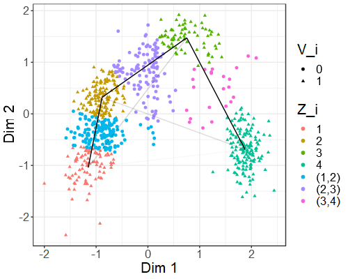
The posterior estimated GARP places 466466466 cells into vertex-clusters (main phases) and 281281281 into ordered edge-clusters (transition phases). Figure 2a summarizes inference. The heat-map in Figure 2b shows the posterior probabilities of co-clustering of pairs of observations, suggesting low posterior uncertainty around the estimated main phases, making the point estimate under the GARP a meaningful posterior summary. The conditional uncertainty of the graph-alignment of the vertices given the point estimates of the main phases is low. Visual inspection of the results suggests that the model is effectively working as expected.
Refer to caption
Refer to caption

(a)                                                                    (b)

Figure 2: Left Panel: Scatter-plot of the scRNA data. Triangular plot symbols indicate cells assigned to vertices (Vi=1subscript𝑉𝑖1V_{i}=1) while the remaining cells are assigned to edges (Vi=0subscript𝑉𝑖0V_{i}=0) and are represented with a circular shape. Cells are colored according to the different phases (i.e., Zisubscript𝑍𝑖Z_{i}) in the point estimate. The segments denote the edges of the graph and the color is darker if the probability of assigning observations to the edge is greater. Right panel: Posterior probabilities of co-clustering of observations assigned to vertices.

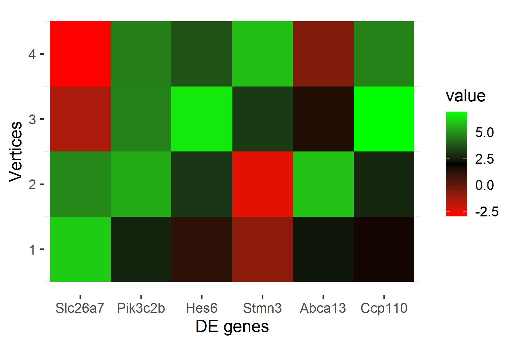
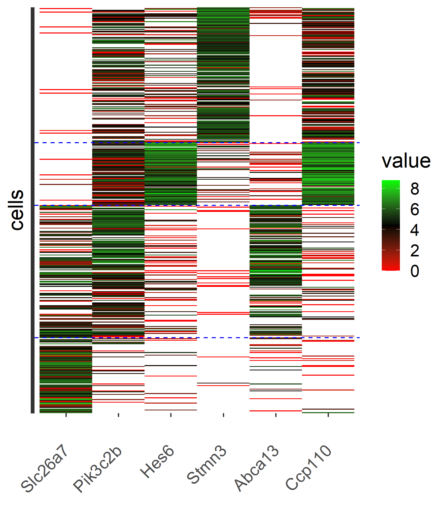
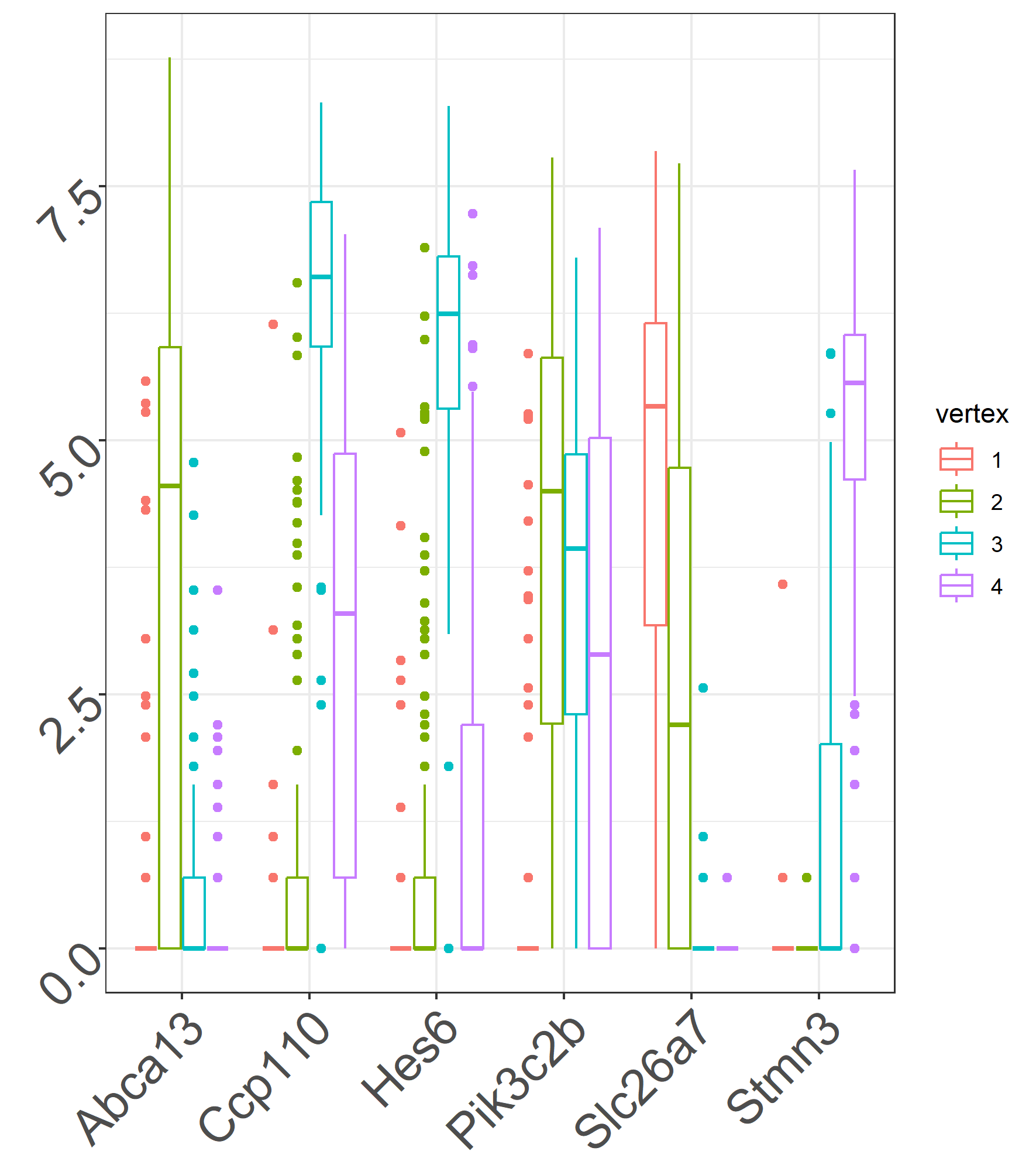
Once we have identified the main phases (vertex-clusters) we find the biomarkers that best characterize such clusters, i.e., the most differently expressed genes (DE genes). We rely on the function findMarkers of the Bioconductor package scran (Lun et al., 2016). More precisely, we first perform an exact binomial test to identify DE genes between pairs of groups of cells (vertex-clusters). From that, we identify the 6 most significant biomarkers for each pairwise comparison. For each gene then a combined p-value is computed using Simes multiplicity adjustment applied to all p-values obtained by the pairwise comparisons (Simes, 1986). Note that these p-values are not directly used for ranking and are only used to find the DE genes. Finally, the p-values are consolidated across all genes using the BH method of Benjamini and Hochberg (1995) to implement multiple comparisons under a restriction on false discovery rate (FDR) (Benjamini et al., 2009). The adjusted p-values are reported in Table 3. The reported FDRs are intended only as a rough measure of significance. Note that properly correcting for multiple testing is not generally possible when clusters are based on the same data that is used for the DE testing. Nonetheless, a small FDR remains desirable. Table 3 shows the average within vertex-cluster gene expressions for the selected top 666 biomarkers and corresponding FDRs. The log means expression in the different biomarkers and vertices are also shown in Figure 3. On average the main phases obtained (vertex-clusters) have very different expressions of the selected biomarkers. Finally, we show the entire distribution of the cells in the different biomarkers and main phases in Figure 4.

DE Genes Vertex 1 Vertex 2 Vertex 3 Vertex 4 FDR
Slc26a7 397.98 142.45 0.27 0.05 1.10e-23
Pik3c2b 19.44 220.70 106.76 98.38 3.81e-08
Hes6 3.00 16.15 669.49 41.62 7.56e-14
Stmn3 0.41 0.08 22.97 320.38 2.89e-21
Abca13 12.98 312.22 5.12 0.54 1.49e-07
Il33 2.77 586.62 8.33 0.85 2.40e-07
Table 3: Average within vertex-cluster gene expressions and FDRs in the selected top 6 biomarkers.
Refer to caption
Figure 3: Heatmap of the log mean expressions in top 6 DE genes in the main phases.
Refer to caption
Refer to caption
Figure 4: Left panel: Heat-map log genetic expressions in top 6 DE genes in all cells ordered by main phases. The cells are sorted by vertex-cluster memberships and the dashed blue lines separate the cells in the different clusters. Right panel: Boxplot genetic expressions (after log(+1)\log(\cdot+1) transformation) in the top 6 DE genes in all cells in the different main phases (vertex-clusters).

7.3 Comparison with Independent Gaussian Mixtures

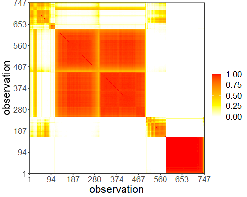
For comparison, we estimate an independent Gaussian mixture model without edges and cluster alignment (implemented as the GARP model with pv=1subscript𝑝𝑣1p_{v}=1). The posterior distribution of the number of clusters (see Table 4) shows more uncertainty since the model fails to find well-separated clusters, due to the noise that is introduced by the presence of the cells transitioning between the main phases. In other words, including cells in transition in the clustering has reduced the statistical power in detecting homogeneous subpopulations. This is illustrated in Figure 5. Recall that we are using VI loss to summarize the posterior random partition. As a consequence of the increased uncertainty, the point estimate of the clustering of the main phases becomes sensitive to the choice of the loss function. For instance, both the point estimate and the maximum a posteriori estimate of the number of main phases is 444 under GARP, while the earlier is 555 and the latter is 666 under the independent Gaussian mixture model. In the figures, we show the estimated cluster arrangement that minimizes the VI loss for coherency in the comparison.

Refer to caption
Refer to caption

(a)                                                                    (b)

Figure 5: Results with independent mixtures. Left Panel: Scatter-plot of the scRNA data. Cells are colored according to the different phases in the point estimate. Right panel: Co-clustering posterior probabilities.
Panel A: GARP
k𝑘k 4 5 6 7 8
P^(Kv=k)^𝑃subscript𝐾𝑣𝑘\hat{P}(K_{v}=k) 0.7801 0.1951 0.0240 0.0004 0.0004
Panel B: Independent Mixture Model
k𝑘k 5 6 7 8 9 10 11 12 13
P^(K=k)^𝑃𝐾𝑘\hat{P}(K=k) 0.0692 0.4362 0.3115 0.114 0.0516 0.0128 0.002 0.0012 0.0016
Table 4: Panel A: Estimated posterior of the number of main phases under GARP.
Panel B: Estimated posterior of the number of main phases under the independent Gaussian mixture model.

8 Discussion

We proposed a graph-aligned random partition model to infer homogeneous subgroups of observations aligned on a graph, explicitly allowing for units transitioning between the clusters. The motivating applications are single-cell RNA experiments where scientists are interested in understanding fundamental biological processes such as cell differentiation and tumor evolution. Interesting future applications include inference for cell type transitions in a tumor microenvironment. Other extensions could include data integration with other modalities, such as histology data.

Methodological extensions include jointly clustering similar cells and genes, via separately exchangeable nested random partition models (Lee et al., 2013b; Lin et al., 2021). Another interesting extension is to combine the results of partially exchangeable random partition models that arise from the compositions of Gibbs-type and species sampling priors (Teh et al., 2006; Camerlenghi et al., 2019; Argiento et al., 2020; Bassetti et al., 2020; Lijoi et al., 2023) to the GARP model with dependent locations. In the context of the scRNA-seq experiment, this would allow inference on multiple single-cell RNA-seq data matrices. In such a way one could borrow information across different measurements while accounting for relevant heterogeneity. Finally, including unit-specific spatial information, the model can be used for spatial clustering with transitions between the clusters.

Acknowledgment

Most of the paper was completed while G. R. was a Postdoc at UT Austin. G. R. was partially funded by NSF/DMS 1952679 and he is also affiliated to the Bocconi Institute for Data Science and Analytics (BIDSA).

References

  • Antoniak (1974) Antoniak, C. E. (1974). Mixtures of Dirichlet processes with applications to Bayesian nonparametric problems. Ann. Stat., 2, 1152–1174.
  • Argiento et al. (2020) Argiento, R., Cremaschi, A., and Vannucci, M. (2020). Hierarchical normalized completely random measures to cluster grouped data. J. Am. Stat. Assoc., 115, 318–333.
  • Bassetti et al. (2020) Bassetti, F., Casarin, R., and Rossini, L. (2020). Hierarchical species sampling models. Bayesian Anal., 15, 809–838.
  • Benjamini and Hochberg (1995) Benjamini, Y. and Hochberg, Y. (1995). Controlling the false discovery rate: a practical and powerful approach to multiple testing. J. R. Stat. Soc. Series B Stat. Methodol., 57, 289–300.
  • Benjamini et al. (2009) Benjamini, Y., Heller, R., and Yekutieli, D. (2009). Selective inference in complex research. Philos. Trans. Royal Soc. A, 367, 4255–4271.
  • Beraha et al. (2022) Beraha, M., Argiento, R., Möller, J., and Guglielmi, A. (2022). MCMC computations for Bayesian mixture models using repulsive point processes. J. Comput. Graph. Stat., 31, 422–435.
  • Betancourt et al. (2022) Betancourt, B., Zanella, G., and Steorts, R. C. (2022). Random partition models for microclustering tasks. J. Am. Stat. Assoc., 117, 1215–1227.
  • Camerlenghi et al. (2019) Camerlenghi, F., Lijoi, A., Orbanz, P., and Prünster, I. (2019). Distribution theory for hierarchical processes. Ann. Stat., 47, 67–92.
  • Dahl et al. (2022) Dahl, D. B., Johnson, D. J., and Müller, P. (2022). Search algorithms and loss functions for Bayesian clustering. J. Comput. Graph. Stat., 31, 1189–1201.
  • De Blasi et al. (2015) De Blasi, P., Favaro, S., Lijoi, A., Mena, R. H., Prünster, I., and Ruggiero, M. (2015). Are Gibbs-type priors the most natural generalization of the Dirichlet process? IEEE Trans. Pattern Anal. Mach. Intell., 37, 212–229.
  • Diaconis and Freedman (1980) Diaconis, P. and Freedman, D. (1980). Finite exchangeable sequences. Ann. Probab., 8, 745–764.
  • Ewens (1990) Ewens, W. J. (1990). Population genetics theory - the past and the future. In S. Lessard, editor, Mathematical and Statistical Developments of Evolutionary Theory, volume 299, pages 177–227. Springer.
  • Gentleman et al. (2004) Gentleman, R. C., Carey, V. J., Bates, D. M., Bolstad, B., Dettling, M., Dudoit, S., Ellis, B., Gautier, L., Ge, Y., Gentry, J., et al. (2004). Bioconductor: open software development for computational biology and bioinformatics. Genome Biol., 5, 1–16.
  • Gnedin (2010) Gnedin, A. V. (2010). A species sampling model with finitely many types. Electron. Commun. Probab., 15, 79–88.
  • Gnedin and Pitman (2006) Gnedin, A. V. and Pitman, J. (2006). Exchangeable Gibbs partitions and Stirling triangles. J. Math. Sci., 138, 5674–5685.
  • Green (2018) Green, P. J. (2018). Introduction to finite mixtures. In S. Fruhwirth-Schnatter, G. Celeux, and C. P. Robert, editors, Handbook of Mixture Analysis, pages 3–20. Chapman and Hall/CRC.
  • Green and Richardson (2001) Green, P. J. and Richardson, S. (2001). Modelling heterogeneity with and without the Dirichlet process. Scand. J. Stat., 28, 355–375.
  • Lee et al. (2013a) Lee, J., Quintana, F. A., Müller, P., and Trippa, L. (2013a). Defining predictive probability functions for species sampling models. Stat. Sci., 28, 209–222.
  • Lee et al. (2013b) Lee, J., Müller, P., Zhu, Y., and Ji, Y. (2013b). A nonparametric Bayesian model for local clustering with application to proteomics. J. Am. Stat. Assoc., 108, 775–788.
  • Lijoi et al. (2005) Lijoi, A., Mena, R. H., and Prünster, I. (2005). Hierarchical mixture modeling with normalized inverse-Gaussian priors. J. Am. Stat. Assoc., 100, 1278–1291.
  • Lijoi et al. (2007a) Lijoi, A., Mena, R. H., and Prünster, I. (2007a). Bayesian nonparametric estimation of the probability of discovering new species. Biometrika, 94, 769–786.
  • Lijoi et al. (2007b) Lijoi, A., Mena, R. H., and Prünster, I. (2007b). Controlling the reinforcement in Bayesian non-parametric mixture models. J. R. Stat. Soc. Series B Stat. Methodol., 69, 715–740.
  • Lijoi et al. (2023) Lijoi, A., Prünster, I., and Rebaudo, G. (2023). Flexible clustering via hidden hierarchical Dirichlet priors. Scand. J. Stat., 50, 213–234.
  • Lin et al. (2021) Lin, Q., Rebaudo, G., and Müller, P. (2021). Separate exchangeability as modeling principle in Bayesian nonparametrics. Preprint at arXiv:2112.07755.
  • Lo (1984) Lo, A. Y. (1984). On a class of Bayesian nonparametric estimates: I. density estimates. Ann. Stat., 12, 351–357.
  • Lun et al. (2016) Lun, A. T., McCarthy, D. J., and Marioni, J. C. (2016). A step-by-step workflow for low-level analysis of single-cell RNA-seq data with Bioconductor. F1000Research, 5, 1–64.
  • Miller and Harrison (2018) Miller, J. W. and Harrison, M. T. (2018). Mixture models with a prior on the number of components. J. Am. Stat. Assoc., 113, 340–356.
  • Neal (2000) Neal, R. M. (2000). Markov chain sampling methods for Dirichlet process mixture models. J. Comput. Graph. Stat., 9, 249–265.
  • Nobile (1994) Nobile, A. (1994). Bayesian Analysis of Finite Mixture Distributions. Ph.D. thesis, Carnegie Mellon Univ.
  • Nobile and Fearnside (2007) Nobile, A. and Fearnside, A. T. (2007). Bayesian finite mixtures with an unknown number of components: the allocation sampler. Stat. Comput., 17, 147–162.
  • Perraudeau et al. (2017) Perraudeau, F., Risso, D., Street, K., Purdom, E., and Dudoit, S. (2017). Bioconductor workflow for single-cell RNA sequencing: normalization, dimensionality reduction, clustering, and lineage inference. F1000Research, 6, 1–28.
  • Petralia et al. (2012) Petralia, F., Rao, V., and Dunson, D. B. (2012). Repulsive mixtures. In Adv. Neural Inf. Process. Syst., volume 25, pages 1889–1897.
  • Pitman (1996) Pitman, J. (1996). Some developments of the Blackwell-MacQueen urn scheme. Lect. Notes-Monogr. Series, 30, 245–267.
  • Pitman and Yor (1997) Pitman, J. and Yor, M. (1997). The two-parameter Poisson-Dirichlet distribution derived from a stable subordinator. Ann. Probab., 25, 855–900.
  • Risso et al. (2018) Risso, D., Perraudeau, F., Gribkova, S., Dudoit, S., and Vert, J.-P. (2018). A general and flexible method for signal extraction from single-cell RNA-seq data. Nat. Commun., 9, 1–17.
  • Simes (1986) Simes, R. J. (1986). An improved Bonferroni procedure for multiple tests of significance. Biometrika, 73, 751–754.
  • Teh et al. (2006) Teh, Y. W., Jordan, M. I., Beal, M. J., and Blei, D. M. (2006). Hierarchical Dirichlet processes. J. Am. Stat. Assoc., 101, 1566–1581.
  • Wade and Ghahramani (2018) Wade, S. and Ghahramani, Z. (2018). Bayesian cluster analysis: point estimation and credible balls (with discussion). Bayesian Anal., 13, 559–626.
  • Xu et al. (2016) Xu, Y., Müller, P., and Telesca, D. (2016). Bayesian inference for latent biologic structure with determinantal point processes (DPP). Biometrics, 72, 955–964.

Supplementary materials of
Graph-Aligned Random Partition Model (GARP)

Giovanni Rebaudoa (giovanni.rebaudo@unito.it)
Peter Müllerb (pmueller@math.utexas.edu)
aCollegio Carlo Alberto & Department of ESOMAS, University of Turin, IT bDepartment of Statistics and Data Sciences & Department of Mathematics,
University of Texas at Austin, USA

S.1 Edge Multivariate Gaussian Mixtures

Figure S.1 shows the contour plot of an edge cluster in 2superscript2\mathbbm{R}^{2}.

Refer to caption
Figure S.1: Elliptical contour plot for an edge-cluster (with hyperparameters, as described in Section S.3), connecting two vertex-clusters k𝑘k and ksuperscript𝑘k^{\prime} (with locations 𝝁1=(2,2)subscript𝝁122\bm{\mu}_{1}=(-2,-2) and 𝝁2=(3,3)subscript𝝁233\bm{\mu}_{2}=(3,3)). The vertices are shown as black bullets located on the contour (not shown) line of the bivariate Gaussian such that 99% of the probability is inside such an ellipse.

Without loss of generality consider an edge connecting the two vertex-clusters, k=1𝑘1k=1 and k=2superscript𝑘2k^{\prime}=2, with cluster-specific parameters 𝝁1superscriptsubscript𝝁1\bm{\mu}_{1}^{\ast} and 𝝁2superscriptsubscript𝝁2\bm{\mu}_{2}^{\ast}. The edge-cluster is centered around the half-point 𝝁1,2=𝝁1+𝝁22superscriptsubscript𝝁12superscriptsubscript𝝁1superscriptsubscript𝝁22\bm{\mu}_{1,2}^{\ast}=\frac{\bm{\mu}_{1}^{\ast}+\bm{\mu}_{2}^{\ast}}{2}. The following construction defines 𝚺1,2subscriptsuperscript𝚺bold-∗12\bm{\Sigma^{\ast}}_{1,2} such that the edge is aligned along the connecting line L1,2subscript𝐿12L_{1,2}, as described in Section 2.1 of the main manuscript. Let 𝒆=𝝁1𝝁2𝝁1𝝁2𝒆superscriptsubscript𝝁1superscriptsubscript𝝁2normsuperscriptsubscript𝝁1superscriptsubscript𝝁2\bm{e}=\frac{\bm{\mu}_{1}^{\ast}-\bm{\mu}_{2}^{\ast}}{||\bm{\mu}_{1}^{\ast}-\bm{\mu}_{2}^{\ast}||}, where 𝝁1𝝁2normsuperscriptsubscript𝝁1superscriptsubscript𝝁2||\bm{\mu}_{1}^{\ast}-\bm{\mu}_{2}^{\ast}|| denotes the Euclidean distance between 𝝁1superscriptsubscript𝝁1\bm{\mu}_{1}^{\ast} and 𝝁2superscriptsubscript𝝁2\bm{\mu}_{2}^{\ast}. Let 𝑷=𝒆𝒆𝑷𝒆superscript𝒆\bm{P}=\bm{e}\bm{e}^{\intercal} be the perpendicular projection matrix such that for any 𝒚ipsubscript𝒚𝑖superscript𝑝\bm{y}_{i}\in\mathbb{R}^{p}, 𝒚i(p)=𝑷𝒚isuperscriptsubscript𝒚𝑖𝑝𝑷subscript𝒚𝑖\bm{y}_{i}^{(p)}=\bm{P}\bm{y}_{i} is the perpendicular projection of 𝒚isubscript𝒚𝑖\bm{y}_{i} onto the connecting line between 𝝁1superscriptsubscript𝝁1\bm{\mu}_{1}^{\ast} and 𝝁2superscriptsubscript𝝁2\bm{\mu}_{2}^{\ast}. Let 𝑷=𝑸𝑫𝑸𝑷𝑸𝑫superscript𝑸\bm{P}=\bm{Q}\bm{D}\bm{Q}^{\intercal} denote a singular value decomposition (SVD) with 𝑫=diag(1,0,,0)𝑫diag100\bm{D}=\text{diag}(1,0,\ldots,0). Thus 𝑹~=𝑸~𝑹superscript𝑸\tilde{\bm{R}}=\bm{Q}^{\intercal} is the rotation matrix such that 𝒚~i=𝑹~𝒚isubscript~𝒚𝑖~𝑹subscript𝒚𝑖\tilde{\bm{y}}_{i}=\tilde{\bm{R}}\bm{y}_{i} is the rotation of 𝒚isubscript𝒚𝑖\bm{y}_{i} in the new axes where the first axis is the line connecting 𝝁1superscriptsubscript𝝁1\bm{\mu}_{1}^{\ast} and 𝝁2superscriptsubscript𝝁2\bm{\mu}_{2}^{\ast} and the others are the orthogonal directions. Now, we define 𝑺~=diag(𝝁1𝝁2r0,r1,,r1)~𝑺diagnormsuperscriptsubscript𝝁1superscriptsubscript𝝁2subscript𝑟0subscript𝑟1subscript𝑟1\tilde{\bm{S}}=\text{diag}(||\bm{\mu}_{1}^{\ast}-\bm{\mu}_{2}^{\ast}||r_{0},r_{1},\ldots,r_{1}) and 𝚺1,2=𝑹~𝑺~𝑹~subscriptsuperscript𝚺bold-∗12bold-~𝑹bold-~𝑺superscriptbold-~𝑹\bm{\Sigma^{\ast}}_{1,2}=\bm{\tilde{R}}\bm{\tilde{S}}\bm{\tilde{R}}^{\intercal}.

Under this construction, the term in the mixture of normal sampling model (1) corresponding to the edge (k,k)𝑘superscript𝑘(k,k^{\prime}) is such that the Gaussian component projected onto the connecting line L1,2subscript𝐿12L_{1,2} has a standard deviation r0𝝁1𝝁2subscript𝑟0normsuperscriptsubscript𝝁1superscriptsubscript𝝁2r_{0}\,||\bm{\mu}_{1}^{\ast}-\bm{\mu}_{2}^{\ast}||, implying lower likelihood for edges between distant vertices’ locations. The standard deviations of the independent Gaussian distributions on the projection onto L1,2superscriptsubscript𝐿12perpendicular-toL_{1,2}^{\perp} is r1subscript𝑟1r_{1}.

S.2 Composition of Discrete Random Probabilities

Let 𝜽i=𝜽Zisubscript𝜽𝑖subscriptsuperscript𝜽bold-∗subscript𝑍𝑖\bm{\theta}_{i}=\bm{\theta^{\ast}}_{Z_{i}} denote the normal moments in the sampling model (1). As a third characterization of the proposed GARP, we define G(N)~~superscript𝐺𝑁\widetilde{G^{(N)}} as a graph-aligned random partition (with unique atoms) implied by the ties under conditional i.i.d. sampling of 𝜽isubscript𝜽𝑖\bm{\theta}_{i}, with separate models for vertex and edge-clusters. For vertex-clusters

𝜽iVi=1,𝑽,PviidPv,Pv=m=1Mvπmδ𝜽~mGibbs-Type Process,formulae-sequenceconditionalsubscript𝜽𝑖subscript𝑉𝑖1𝑽subscript𝑃𝑣iidsimilar-tosubscript𝑃𝑣subscript𝑃𝑣superscriptsubscript𝑚1subscript𝑀𝑣subscript𝜋𝑚subscript𝛿subscriptbold-~𝜽𝑚similar-toGibbs-Type Process\displaystyle\begin{split}&\bm{\theta}_{i}\mid V_{i}=1,\bm{V},P_{v}\overset{\text{iid}}{\sim}P_{v},\\ &P_{v}=\sum_{m=1}^{M_{v}}\pi_{m}\delta_{\bm{\tilde{\theta}}_{m}}\sim\text{Gibbs-Type Process},\end{split} (S.1)

where Mvsubscript𝑀𝑣M_{v} is the number of atoms of the discrete random probability Pvsubscript𝑃𝑣P_{v} that is a Gibbs-type process and can be finite, as in the finite symmetric DM case, infinite as in the DP and PYP case, or be a random variable on \mathbb{N} as in the MFM case. Thus (πm)m=1Mvsuperscriptsubscriptsubscript𝜋𝑚𝑚1subscript𝑀𝑣(\pi_{m})_{m=1}^{M_{v}} are the random weights (that are sampled independently from the atoms) from the distribution on the simplex associated with the Gibbs-type process. The unique atoms 𝜽~msubscriptbold-~𝜽𝑚\bm{\tilde{\theta}}_{m} of Pvsubscript𝑃𝑣P_{v} are i.i.d. samples from the NIW distribution in (2). Note that the unique sampled vertex parameters 𝜽v={𝜽1,,𝜽Kv}subscriptsuperscript𝜽bold-∗𝑣subscriptsuperscript𝜽bold-∗1subscriptsuperscript𝜽bold-∗subscript𝐾𝑣\bm{\theta^{\ast}}_{v}=\{\bm{\theta^{\ast}}_{1},\ldots,\bm{\theta^{\ast}}_{K_{v}}\} are a subset of {𝜽1~,,𝜽~Mv}~subscript𝜽1subscript~𝜽subscript𝑀𝑣\{\tilde{\bm{\theta}_{1}},\ldots,\tilde{\bm{\theta}}_{M_{v}}\}.

The edge-clusters are implied by

𝜽iVi=0,𝑽i,Kv,𝜽viidPe,Pe=1k<kKvπk,kδ(𝜽k,k).formulae-sequenceconditionalsubscript𝜽𝑖subscript𝑉𝑖0superscript𝑽𝑖subscript𝐾𝑣subscriptsuperscript𝜽bold-∗𝑣iidsimilar-tosubscript𝑃𝑒subscript𝑃𝑒subscript1𝑘superscript𝑘subscript𝐾𝑣subscript𝜋𝑘superscript𝑘subscript𝛿subscriptsuperscript𝜽bold-∗𝑘superscript𝑘\displaystyle\begin{split}&\bm{\theta}_{i}\mid V_{i}=0,\bm{V}^{-i},K_{v},\bm{\theta^{\ast}}_{v}\overset{\text{iid}}{\sim}P_{e},\\ &P_{e}=\sum_{1\leq k<k^{\prime}\leq K_{v}}\pi_{k,k^{\prime}}\delta_{(\bm{\theta^{\ast}}_{k,k^{\prime}})}.\end{split} (S.2)

Recall that Me=Kv(Kv1)/2subscript𝑀𝑒subscript𝐾𝑣subscript𝐾𝑣12M_{e}=K_{v}(K_{v}-1)/2. The random weights follow a symmetric Mesubscript𝑀𝑒M_{e}-dimensional Dirichlet with hyper-parameter β/Me𝛽subscript𝑀𝑒\beta/M_{e},

(πk,k)1k<kKvDir(β/Me,,β/Me).similar-tosubscriptsubscript𝜋𝑘superscript𝑘1𝑘superscript𝑘subscript𝐾𝑣Dir𝛽subscript𝑀𝑒𝛽subscript𝑀𝑒(\pi_{k,k^{\prime}})_{1\leq k<k^{\prime}\leq K_{v}}\sim\text{Dir}(\beta/M_{e},\ldots,\beta/M_{e}). (S.3)

From the characterizations of Gibbs-type and DM processes, it is straightforward to show that the aforementioned discrete conditional random probability models for the parameters characterize the GARP as stated in the following proposition.

Proposition S.5.

The random partition structure of the GARP model (4) and the vertex- and edge-parameters distributions can be characterized as the configuration of ties implied by the truncation sampling model in (7), (8), (S.1), (S.2), and (S.3).

S.3 Hyperparameters Settings

In both the application and the simulation we set γ=0.5𝛾0.5\gamma=0.5 for the Gnedin process controlling the vertex-clusters and β=0.5𝛽0.5\beta=0.5 for the symmetric DM with hyperparameter 0.5/Mv0.5subscript𝑀𝑣0.5/M_{v} to favor the sparsity of the graph. Moreover, for the choice of the hyperparameters of the NIW we set 𝝁0=𝒚¯subscript𝝁0¯𝒚\bm{\mu}_{0}=\bar{\bm{y}}, κ0=0.001subscript𝜅00.001\kappa_{0}=0.001 ν0=100subscript𝜈0100\nu_{0}=100 𝚲0=ξ2𝐈subscript𝚲0superscript𝜉2𝐈\mathbf{\Lambda}_{0}=\xi^{2}\,\mathbf{I} and 𝚺0=𝚲01subscript𝚺0superscriptsubscript𝚲01\bm{\Sigma}_{0}=\mathbf{\Lambda}_{0}^{-1}. For scenarios in which the cluster are well separated, we recommend a large value of ξ2superscript𝜉2\xi^{2} (that we set equal to 150150150), while we recommend a smaller value of ξ2superscript𝜉2\xi^{2} (that we set equal to 151515) if the data are not well separated in the Euclidean space. Moreover, in both the application and the simulation we set r02=4(χ2,1α2)1superscriptsubscript𝑟024superscriptsuperscriptsubscript𝜒21𝛼21r_{0}^{2}=4(\chi_{2,1-\alpha}^{2})^{-1} and r12=(2χ2,1α2)1superscriptsubscript𝑟12superscript2superscriptsubscript𝜒21𝛼21r_{1}^{2}=(2\chi_{2,1-\alpha}^{2})^{-1}, where χ2,1α2superscriptsubscript𝜒21𝛼2\chi_{2,1-\alpha}^{2} is the quantile of order 1α1𝛼1-\alpha (we set α=1%𝛼percent1\alpha=1\%) of a Chi-squared distribution with 2 degrees of freedom to have the desired eccentricity of the elliptical contour plot of the edge as well as the 99%percent9999\%-level of the contour plot not too spread. To obtain that, recall that c𝑐c-level counter-plot of multivariate Gaussian density, such as the edge Gaussian in (1), are points 𝒚d𝒚superscript𝑑\bm{y}\in\mathbbm{R}^{d} such that (𝒚𝝁k,k)𝚺k,k1(𝒚𝝁k,k)superscript𝒚subscript𝝁𝑘superscript𝑘superscriptsubscript𝚺𝑘superscript𝑘1𝒚subscript𝝁𝑘superscript𝑘(\bm{y}-\bm{\mu}_{k,k^{\prime}})^{\intercal}\bm{\Sigma}_{k,k^{\prime}}^{-1}(\bm{y}-\bm{\mu}_{k,k^{\prime}}) is constant, that is the contour levels are ellipsoid centered at 𝝁k,ksubscript𝝁𝑘superscript𝑘\bm{\mu}_{k,k^{\prime}}. Finally, note that if 𝒚N(𝝁k,k,𝚺k,k)similar-to𝒚Nsubscript𝝁𝑘superscript𝑘subscript𝚺𝑘superscript𝑘\bm{y}\sim\text{N}(\bm{\mu}_{k,k^{\prime}},\bm{\Sigma}_{k,k^{\prime}}) then,

(𝒚𝝁k,k)𝚺k,k1(𝒚𝝁k,k)χd2,similar-tosuperscript𝒚subscript𝝁𝑘superscript𝑘superscriptsubscript𝚺𝑘superscript𝑘1𝒚subscript𝝁𝑘superscript𝑘subscriptsuperscript𝜒2𝑑(\bm{y}-\bm{\mu}_{k,k^{\prime}})^{\intercal}\bm{\Sigma}_{k,k^{\prime}}^{-1}(\bm{y}-\bm{\mu}_{k,k^{\prime}})\sim\chi^{2}_{d}\,,

where χd2subscriptsuperscript𝜒2𝑑\chi^{2}_{d} denotes the Chi-square distribution with d𝑑d degrees of freedom.

Visually the contour plots of such edge density are shown in Figure S.1 and the data sampled from such configuration looks like the one in Figure S.2.
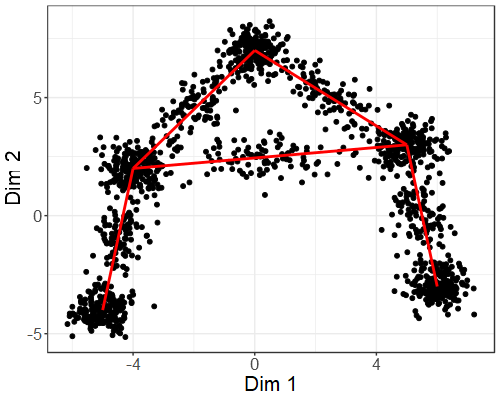
Refer to caption
Figure S.2: Scatter-plot of the simulated data. The red segments represent the edges that connect the truth vertices.

S.4 Implementing Posterior Inference

S.4.1 Use of the Relaxed Model G(N)~~superscript𝐺𝑁\widetilde{G^{(N)}} in Posterior Simulation

We discuss in more detail the use of the projectivity property of G(N)~~superscript𝐺𝑁\widetilde{G^{(N)}} to define a Pólya urn scheme for a tractable marginal posterior simulation algorithm. First, recall that the relaxed model G(N)~~superscript𝐺𝑁\widetilde{G^{(N)}} can be seen as a hierarchical composition of a Kolmogorov consistent EPPFs with product partition forms (Sections 2.2 and 3), which implies tractable expressions for G(N)~(Vi,Zi𝑽i,𝒁i)=G(N)~(𝑽,𝒁)G(N)~(𝑽i,𝒁i)~superscript𝐺𝑁subscript𝑉𝑖conditionalsubscript𝑍𝑖superscript𝑽𝑖superscript𝒁𝑖~superscript𝐺𝑁𝑽𝒁~superscript𝐺𝑁superscript𝑽𝑖superscript𝒁𝑖\widetilde{G^{(N)}}(V_{i},Z_{i}\mid\bm{V}^{{}^{-i}},\bm{Z}^{{}^{-i}})=\frac{\widetilde{G^{(N)}}(\bm{V},\bm{Z})}{\widetilde{G^{(N)}}(\bm{V}^{{}^{-i}},\bm{Z}^{{}^{-i}})} under the relaxed model G(N)~~superscript𝐺𝑁\widetilde{G^{(N)}}.

To derive then the desired full conditional distributions under G(N)superscript𝐺𝑁G^{(N)} we note, e.g., that if Ii=0subscript𝐼𝑖0I_{i}=0 for (𝑽,𝒁)𝑽𝒁(\bm{V},\bm{Z}) (recall the definition of Iisubscript𝐼𝑖I_{i} in Section 6), then

G(N){Vi=v,Zi=z}G(N)~(𝑽,𝒁)j[N]N(𝒚j𝜽Zj)G(N)~(𝑽i,𝒁i)j[N]iN(𝒚j𝜽Zj),proportional-tosuperscript𝐺𝑁conditional-setformulae-sequencesubscript𝑉𝑖𝑣subscript𝑍𝑖𝑧~superscript𝐺𝑁𝑽𝒁subscriptproduct𝑗delimited-[]𝑁Nconditionalsubscript𝒚𝑗subscriptsuperscript𝜽bold-∗subscript𝑍𝑗~superscript𝐺𝑁superscript𝑽𝑖superscript𝒁𝑖subscriptproduct𝑗superscriptdelimited-[]𝑁𝑖Nconditionalsubscript𝒚𝑗subscriptsuperscript𝜽bold-∗subscript𝑍𝑗G^{(N)}\{V_{i}=v,Z_{i}=z\mid\cdots\}\propto\dfrac{\widetilde{G^{(N)}}(\bm{V},\bm{Z})\prod_{j\in[N]}\text{N}(\bm{y}_{j}\mid\bm{\theta^{\ast}}_{Z_{j}})}{\widetilde{G^{(N)}}(\bm{V}^{{}^{-i}},\bm{Z}^{{}^{-i}})\prod_{j\in[N]^{{}^{-i}}}\text{N}(\bm{y}_{j}\mid\bm{\theta^{\ast}}_{Z_{j}})},

for any v{0,1}𝑣01v\in\{0,1\} and z𝒁i𝑧superscript𝒁𝑖z\in\bm{Z}^{{}^{-i}}. Moreover, when Ii=0subscript𝐼𝑖0I_{i}=0 for (𝑽,𝒁)𝑽𝒁(\bm{V},\bm{Z}), the marginal probability in the denominator is equal to the one in a Kolmogorov consistent model (i.e., if Ii=0subscript𝐼𝑖0I_{i}=0, G(N)~(𝑽i,𝒁i)=G(N1)~(𝑽i,𝒁i)~superscript𝐺𝑁superscript𝑽𝑖superscript𝒁𝑖~superscript𝐺𝑁1superscript𝑽𝑖superscript𝒁𝑖\widetilde{G^{(N)}}(\bm{V}^{{}^{-i}},\bm{Z}^{{}^{-i}})=\widetilde{G^{(N-1)}}(\bm{V}^{{}^{-i}},\bm{Z}^{{}^{-i}}), up to a normalization constant) and this allows us to generalize then tractable marginal samplers such as in Neal (2000) or Teh et al. (2006) relying on the characterization of the GARP via a composition of gCRP in Section 2.3.

S.4.2 Point Estimates for the GARP Random Partition

How to choose good summaries (i.e., point estimates) for reporting posterior inference on functionals of interest can be a fundamental and nontrivial question in Bayesian analysis. It is especially challenging if the object of interest is a partition or a graph. To define a posterior point estimate and perform uncertainty quantification we build on the existing literature of posterior point estimates of random partition based on a decision-theoretic approach (Wade and Ghahramani, 2018; Dahl et al., 2022b) generalizing the results for the more challenging case of GARP. We propose a point estimate for the GARP as follows.

(1) Assign observations to vertices versus edges using the posterior mode,

V^i=1 if V¯itVi(t)T>0.5,subscript^𝑉𝑖1 if subscript¯𝑉𝑖subscript𝑡superscriptsubscript𝑉𝑖𝑡𝑇0.5\hat{V}_{i}=1\text{ if }\bar{V}_{i}\equiv\sum_{t}\frac{V_{i}^{(t)}}{T}>0.5,

where T𝑇T is the Monte Carlo sample size, and Vi(t)superscriptsubscript𝑉𝑖𝑡V_{i}^{(t)} is the imputed value in iteration t𝑡t of the MCMC simulations. The uncertainty around the point estimate is quantified using (1V^i)V¯i+V^i(1V¯i)1subscript^𝑉𝑖subscript¯𝑉𝑖subscript^𝑉𝑖1subscript¯𝑉𝑖(1-\hat{V}_{i})\bar{V}_{i}+\hat{V}_{i}(1-\bar{V}_{i}).

(2) Given 𝑽^^𝑽\hat{\bm{V}} we find a point estimate 𝒁^vsubscriptbold-^𝒁𝑣\bm{\hat{Z}}_{v} for the partition of vertex units by minimizing the variation of information loss (Meilă, 2007) as suggested by Wade and Ghahramani (2018) and implemented in the R package salso (Dahl et al., 2022a). Alternative loss functions can be used as needed for different applications (See e.g., Binder, 1978). For uncertainty quantification, we report the heat-map with the posterior probabilities of co-clustering.

(3) Given 𝑽^^𝑽\hat{\bm{V}} and 𝒁^vsubscriptbold-^𝒁𝑣\bm{\hat{Z}}_{v} we find a point estimate 𝒁^esubscriptbold-^𝒁𝑒\bm{\hat{Z}}_{e} and conditional uncertainty quantification for 𝒁𝒆subscript𝒁𝒆\bm{Z_{e}} using the posterior probability of observations being assigned to the different edges. We evaluate conditional posterior probabilities of assigning the remaining observations to the possible edges,

G(𝒁𝒆)k<kΓ(nk,k+β/Me)Ck,kN(𝒚i𝝁k,k,v𝚺k,k).proportional-to𝐺conditionalsubscript𝒁𝒆subscriptproduct𝑘superscript𝑘Γsubscript𝑛𝑘superscript𝑘𝛽subscript𝑀𝑒subscriptproductsubscript𝐶𝑘superscript𝑘Nconditionalsubscript𝒚𝑖superscriptsubscript𝝁𝑘superscript𝑘𝑣superscriptsubscript𝚺𝑘superscript𝑘G(\bm{Z_{e}}\mid\cdots)\propto\prod_{k<k^{\prime}}\Gamma(n_{k,k^{\prime}}+\beta/M_{e})\prod_{C_{k,k^{\prime}}}\text{N}(\bm{y}_{i}\mid\bm{\mu}_{k,k^{\prime}}^{\ast},v\bm{\Sigma}_{k,k^{\prime}}^{\ast}). (S.4)

Here the first product goes over all (k,k)𝑘superscript𝑘(k,k^{\prime}) with 1k<kKv1𝑘superscript𝑘subscript𝐾𝑣1\leq k<k^{\prime}\leq K_{v} and the second over the 𝒚isubscript𝒚𝑖\bm{y}_{i} such that zi=(k,k)subscript𝑧𝑖𝑘superscript𝑘z_{i}=(k,k^{\prime}), i.e., the set Ck,ksubscript𝐶𝑘superscript𝑘C_{k,k^{\prime}}. Probabilities (S.4) are evaluated by Rao-Blackwellization (Robert and Roberts, 2021), using the full conditionals

G{Zi=(k,k)Vi=0,}(nk,ki+β/Me)Norm(𝒚i𝝁k,k,𝚺k,k).proportional-to𝐺conditional-setsubscript𝑍𝑖𝑘superscript𝑘subscript𝑉𝑖0subscriptsuperscript𝑛𝑖𝑘superscript𝑘𝛽subscript𝑀𝑒Normconditionalsubscript𝒚𝑖superscriptsubscript𝝁𝑘superscript𝑘superscriptsubscript𝚺𝑘superscript𝑘G\{Z_{i}=(k,k^{\prime})\mid V_{i}=0,\cdots\}\propto(n^{-i}_{k,k^{\prime}}+\beta/M_{e})\text{Norm}(\bm{y}_{i}\mid\bm{\mu}_{k,k^{\prime}}^{\ast},\bm{\Sigma}_{k,k^{\prime}}^{\ast}).

We visualize p(𝒁𝒆𝒁^v,𝝁,𝚺)𝑝conditionalsubscript𝒁𝒆subscriptbold-^𝒁𝑣superscript𝝁superscript𝚺p(\bm{Z_{e}}\mid\bm{\hat{Z}}_{v},\,\bm{\mu}^{\ast},\,\bm{\Sigma}^{\ast}) by adding edges between vertices with color intensity proportional to the sum over observations assigned to edges (i.e., V^i=0subscript^𝑉𝑖0\hat{V}_{i}=0) of the probability that such observations will be assigned to the different edges (k,k)𝑘superscript𝑘(k,k^{\prime})’s.

S.5 Simulation Studies

We carried out a simulation study under a well-specified and a miss-specified data generating truth to assess inference under finite sample size scenarios. We set up simulation truths close to the mouse data. The data are simulated from a 5 vertex mixture with nk=200subscript𝑛𝑘200n_{k}=200 observations in each vertex and an additional nk,k=100subscript𝑛𝑘superscript𝑘100n_{k,k^{\prime}}=100 observations around 5 assumed edges.

S.5.1 Well Specified Scenario

In the first simulation scenario, we assume a simulation truth with Kv=5subscript𝐾𝑣5K_{v}=5 vertex clusters with cluster-specific Gaussians with mean vectors (5,4)54(-5,-4), (4,2)42(-4,2), (0,7)07(0,7), (5,3)53(5,3) and (6,3)63(6,-3), and a common covariance matrix diag(0.25,0.25)diag0.250.25\text{diag}(0.25,0.25). Observations assigned to edge components are sampled from a Gaussian mixture with cluster-specific kernels as in (3). The simulated N=1500𝑁1500N=1500 observations are shown in Figure S.3a.

Figure S.3 shows that the GARP was able to recover the simulated truth in the point estimate. Moreover, the uncertainty around the point estimate is low.
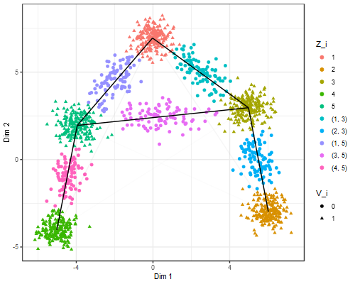
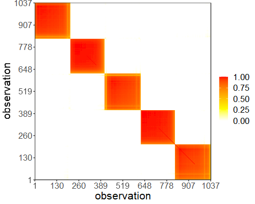
Refer to caption
Refer to caption

(a)                                                                  (b)

Figure S.3: Well-specified simulation scenario. Left Panel: Scatter plot of the simulated data. Observations are colored according to the estimated cluster membership. Line segments show edges of the estimated graph, with the clusters at the end of line segments being vertex clusters, and clusters along the line segments being edge clusters. The grey level of the line segments shows the estimated probability of assigning observations to the respective edge (barely varying in this case). Right panel: Posterior co-clustering probabilities for all observations assigned to vertices.

S.5.2 Misspecified Scenario

Here we consider a misspecified data-generating truth, using the same true mean vectors for five vertex clusters with cluster-specific Gaussian kernels as in the previous scenario, but inflated vertex-specific covariance matrices diag(0.5,0.5)diag0.50.5\text{diag}(0.5,0.5). For the edge components, we introduce two sources of misspecification. First, we center the edge components not at the midpoint of the two adjacent vertices but introduce a bias term. Instead, the edge-specific kernels are centered at 𝝁k+𝝁k2subscriptsuperscript𝝁bold-∗𝑘subscriptsuperscript𝝁bold-∗superscript𝑘2\frac{\bm{\mu^{\ast}}_{k}+\bm{\mu^{\ast}}_{k^{\prime}}}{2} plus a shift of +0.250.25+0.25 in the direction of the line connecting the adjacent vertices, as well as in the perpendicular direction. Second, the observations for the edge components are generated from a uniform distribution on a rectangle centered at the described 𝝁k,ksubscriptsuperscript𝝁bold-∗𝑘superscript𝑘\bm{\mu^{\ast}}_{k,k^{\prime}} and with the length of the side in the direction of the connecting line equal to half the length of the Euclidean distance between the adjacent vertices and the length of the other side equals 222. Under this simulation truth, the scatter plot of the simulated data still allows a meaningful definition of vertex and edge clusters, but the additional misspecification and variability with respect to the well-specified scenario make the inference with our model more challenging. The simulated N=1500𝑁1500N=1500 observations are shown in Figure S.4a.

Figure S.4 shows that the GARP was able to recover well the simulated truth in the point estimate in this misspecified scenario. The uncertainty around the point estimate is low.
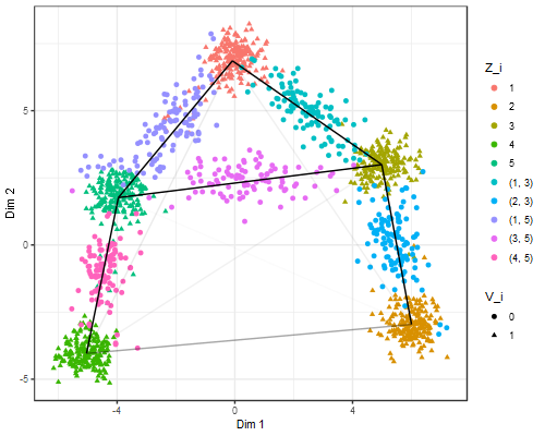
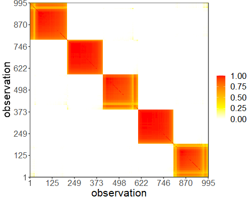
Refer to caption
Refer to caption

(a)                                                                  (b)     

Figure S.4: Mis-specified simulation scenario. Left Panel: Scatter plot of the simulated data. Observations are colored according to estimated cluster membership. The line segments denote estimated edges, with clusters at the end of the line segments being vertex clusters, and clusters along the line segments being edge clusters. The gray shade of the line segments indicates the probability of assigning observations to the respective edge. Right panel: Posterior co-clustering probabilities for observations assigned to vertices.

S.5.3 Non-Connected Graph Scenario

Here we investigate how the model works in a scenario with no meaningful notion of the connected graph in the data. More precisely, we simulate from a mixture of five vertex clusters, exactly as in Section S.5.1, but without any edge components.

The simulated N=1000𝑁1000N=1000 observations and inference under the GARP are shown in Figure S.5a.
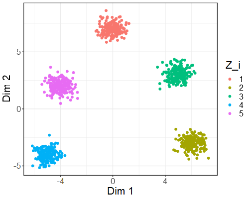
Refer to caption
Refer to caption

(a)                                                                  (b)

Figure S.5: Non-connected graph simulated data. Left Panel: Scatter plot of the simulated data. Observations are colored according to estimated cluster membership. Correctly recovering the simulation truth there are no estimated edge clusters. Right panel: Posterior co-clustering probabilities.

Figure S.5 shows that the GARP was able to recover well the simulated truth in the point estimate also under this not connected graph simulation truth.

S.6 Proof of the Main Results

For easy reference, we provide in Table S.1 a brief statement of the various probability models used in the discussion and the results, and in the following list a brief summary of the main results. Here, Ex. 14 refer to the four examples for the EPPF from Section 3.

G(N)superscript𝐺𝑁G^{(N)} GARP model (4)
G(N)~~superscript𝐺𝑁\widetilde{G^{(N)}} relaxed model (7), G(N)~~superscript𝐺𝑁\widetilde{G^{(N)}} is proportional to G(N)superscript𝐺𝑁G^{(N)}, but w/o 𝟙(EN)1subscript𝐸𝑁\mathbbm{1}(E_{N})
GVZ(N)~~superscriptsubscript𝐺VZ𝑁\widetilde{G_{\mbox{\tiny VZ}}^{(N)}} law under G(N)~~superscript𝐺𝑁\widetilde{G^{(N)}} on (Ti,i=1,,N)formulae-sequencesubscript𝑇𝑖𝑖1𝑁(T_{i},\,i=1,\ldots,N), Ti={Viif Vi=0(Vi,Zi)if Vi=1subscript𝑇𝑖casessubscript𝑉𝑖if subscript𝑉𝑖0subscript𝑉𝑖subscript𝑍𝑖if subscript𝑉𝑖1T_{i}=\begin{cases}V_{i}&\mbox{if }V_{i}=0\\ (V_{i},Z_{i})&\mbox{if }V_{i}=1\end{cases}
GVZ~~subscript𝐺VZ\widetilde{G_{\mbox{\tiny VZ}}} Kolmogorov-consistent extension of GVZ(N)~~superscriptsubscript𝐺VZ𝑁\widetilde{G_{\mbox{\tiny VZ}}^{(N)}} to N𝑁N\in\mathbbm{N}
G()superscript𝐺G^{(\infty)} inf exch. law that eventually matches prior predictives under Ex 1 or 2 (or any MFM)
GN()subscriptsuperscript𝐺𝑁G^{(\infty)}_{N} marginal law under G()superscript𝐺G^{(\infty)}
Table S.1: Probability models used in the discussion and main results

For notational simplicity, we refer with GVZ~~subscript𝐺VZ\widetilde{G_{\mbox{\tiny VZ}}} also to the marginal laws of the stochastic process (Ti)isubscriptsubscript𝑇𝑖𝑖(T_{i})_{i\in\mathbb{N}} as well as the law of Mvsubscript𝑀𝑣M_{v} and (πm)m=1Mvsuperscriptsubscriptsubscript𝜋𝑚𝑚1subscript𝑀𝑣(\pi_{m})_{m=1}^{M_{v}} in (S.1) since they do not depend on the dimension N𝑁N. Finally, we refer with G(N)superscript𝐺𝑁G^{(N)} to the probability density and mass functions of random variables under the GARP models (1)–(4).

Propositions 1 and S.5:

Characterizations of the GARP G(N)superscript𝐺𝑁G^{(N)} as truncation of G(N)~~superscript𝐺𝑁\widetilde{G^{(N)}}, which in turn is characterized as (i) a gCRP or, (ii) a composition of random discrete prob measures, respectively.

Proposition 2:

Analytical statement of G(N)~{EN}~superscript𝐺𝑁subscript𝐸𝑁\widetilde{G^{(N)}}\{E_{N}\} for a general Gibbs-type prior.

Theorem 1:

Let g=limNG(N)~{Kv=1}superscript𝑔subscript𝑁~superscript𝐺𝑁subscript𝐾𝑣1g^{\infty}=\lim_{N\rightarrow\infty}\widetilde{G^{(N)}}{\{K_{v}=1\}} and gv=limnvG(N)~{Kv=1Nv=nv}superscriptsubscript𝑔𝑣subscriptsubscript𝑛𝑣~superscript𝐺𝑁conditional-setsubscript𝐾𝑣1subscript𝑁𝑣subscript𝑛𝑣g_{v}^{\infty}=\lim_{n_{v}\rightarrow\infty}\widetilde{G^{(N)}}\{K_{v}=1\mid N_{v}=n_{v}\}. Then

g=gv={0Ex 1 , 34γ(0,1)Ex 2superscript𝑔subscriptsuperscript𝑔𝑣cases0Ex 1 , 34𝛾01Ex 2g^{\infty}=g^{\infty}_{v}=\begin{cases}0&\mbox{Ex \ref{ex: sym dir} , \ref{ex: DP}, \ref{ex: PYP}}\\ \gamma\in(0,1)&\mbox{Ex \ref{ex: GP}}\end{cases}
Theorem 2:

GVZ~{EN eventually}={1Ex 1 , 341GVZ~{Mv=1}Ex 2~subscript𝐺VZsubscript𝐸𝑁 eventuallycases1Ex 1 , 341~subscript𝐺VZsubscript𝑀𝑣1Ex 2\widetilde{G_{\mbox{\tiny VZ}}}\{E_{N}\text{ eventually}\}=\begin{cases}1&\mbox{Ex \ref{ex: sym dir} , \ref{ex: DP}, \ref{ex: PYP}}\\ 1-\widetilde{G_{\mbox{\tiny VZ}}}\{M_{v}=1\}&\mbox{Ex \ref{ex: GP}}\end{cases}.

Proposition 3:

fEPPFK(N)subscriptsuperscriptfEPPF𝑁𝐾\text{fEPPF}^{(N)}_{K} under the GARP model in (4).

Proposition 4:

The data 𝒚𝒚\bm{y}, the graph-aligned random partition induced by (Vi,Zi)subscript𝑉𝑖subscript𝑍𝑖(V_{i},Z_{i}) and the random partition ΨNsubscriptΨ𝑁\Psi_{N} are finitely exchangeable, but not a projection of an infinitely exchangeable process under our proposal (1)–(4).

Theorem 3 and Corollary 1:

Under Ex 1, the prior predictive probabilities for Vi,Zisubscript𝑉𝑖subscript𝑍𝑖V_{i},Z_{i} under the GARP are eventually equal to the same under a Kolmogorov-consistent sequence (GN())subscriptsuperscript𝐺𝑁\big{(}G^{(\infty)}_{N}\big{)}; statement of a Pólya urn and directing measure for (GN())subscriptsuperscript𝐺𝑁\big{(}G^{(\infty)}_{N}\big{)}.
The same remains true for any MFM.

S.6.1 Proof of Proposition 1

Proof.

We assume the GARP definition via the relaxed model in (7), (8), (9), and (10) and show that is equivalent to the definition in (4).

First, we note that in (4) the constraint 𝟙(EN)1subscript𝐸𝑁\mathbbm{1}(E_{N}) can be rewritten as 𝟙({Nv=N}{Kv>1})1subscript𝑁𝑣𝑁subscript𝐾𝑣1\mathbbm{1}(\{N_{v}=N\}\cup\{K_{v}>1\}). Note also that under Ne=0subscript𝑁𝑒0N_{e}=0 the second line in (4) does not arise. For notational simplicity, we naturally extend the definition of Kvsubscript𝐾𝑣K_{v} and Mesubscript𝑀𝑒M_{e} by defining Kv=Me=0subscript𝐾𝑣subscript𝑀𝑒0K_{v}=M_{e}=0 if Nv=0subscript𝑁𝑣0N_{v}=0 and defining DM(0)()=DM0()()1superscriptsubscriptDM0superscriptsubscriptDM01\text{DM}_{\cdot}^{(0)}(\cdot)=\text{DM}_{0}^{(\cdot)}(\cdot)\equiv 1.

Note also that (9) is equivalent to sample 𝒁v=(Zi:i[N],Vi=1)\bm{Z}_{v}=(Z_{i}:i\in[N],\,V_{i}=1) from

G(N)~(𝒁𝒗𝑽)=EPPFKv(Nv)(n1,,nKvα,σ)/Kv!~superscript𝐺𝑁conditionalsubscript𝒁𝒗𝑽superscriptsubscriptEPPFsubscript𝐾𝑣subscript𝑁𝑣subscript𝑛1conditionalsubscript𝑛subscript𝐾𝑣𝛼𝜎subscript𝐾𝑣\widetilde{G^{(N)}}(\bm{Z_{v}}\mid\bm{V})=\mathrm{EPPF}_{K_{v}}^{(N_{v})}(n_{1},\ldots,n_{K_{v}}\mid\alpha,\sigma)/K_{v}! (S.5)

The clustering indicators Zisubscript𝑍𝑖Z_{i} are a 1-to-1 mapping of the induced exchangeable random partition up to possible relabelings. By (conditional) exchangeability of the partition, any possible relabeling of 𝒁𝒗subscript𝒁𝒗\bm{Z_{v}} has the same probability that is equal to the EPPF divided by the number of relabelings, i.e., Kv!subscript𝐾𝑣K_{v}!.

Similarly, sampling from (10) is equivalent to sample 𝒁𝒆=(Zi:i[N],Vi=0)\bm{Z_{e}}=(Z_{i}:i\in[N],\,V_{i}=0) from

G(N)~(𝒁𝒆𝒁𝒗)=DMMe(Ne)((nk,k)k<kvβ/Me),~superscript𝐺𝑁conditionalsubscript𝒁𝒆subscript𝒁𝒗superscriptsubscriptDMsubscript𝑀𝑒subscript𝑁𝑒conditionalsubscriptsubscript𝑛𝑘superscript𝑘𝑘superscriptsubscript𝑘𝑣𝛽subscript𝑀𝑒\displaystyle\widetilde{G^{(N)}}(\bm{Z_{e}}\mid\bm{Z_{v}})=\text{DM}_{M_{e}}^{(N_{e})}((n_{k,k^{\prime}})_{k<k_{v}^{\prime}}\mid\beta/M_{e}),

where DMMe(Ne)((nk,k)k<kv)superscriptsubscriptDMsubscript𝑀𝑒subscript𝑁𝑒subscriptsubscript𝑛𝑘superscript𝑘𝑘superscriptsubscript𝑘𝑣\text{DM}_{M_{e}}^{(N_{e})}((n_{k,k^{\prime}})_{k<k_{v}^{\prime}}) denotes the marginal likelihood of the DM distribution for the categorical random variables, which is a function of the sufficient statistics (nk,k)k<kvsubscriptsubscript𝑛𝑘superscript𝑘𝑘superscriptsubscript𝑘𝑣(n_{k,k^{\prime}})_{k<k_{v}^{\prime}}, i.e., the ordered cardinalities of the different edges. In contrast to the EPPF and fEPPF, here some nk,ksubscript𝑛𝑘superscript𝑘n_{k,k^{\prime}} can be 00, implying that there is no edge connecting the vertices k𝑘k and ksuperscript𝑘k^{\prime}.

Finally, we obtain (4) via the multiplication rule of probability, i.e.,

G(N)~(𝑽,𝒁)=G(N)~(𝑽)G(N)~(𝒁𝒗𝑽)G(N)~(𝒁𝒆𝑽,𝒁𝒗)~superscript𝐺𝑁𝑽𝒁~superscript𝐺𝑁𝑽~superscript𝐺𝑁conditionalsubscript𝒁𝒗𝑽~superscript𝐺𝑁conditionalsubscript𝒁𝒆𝑽subscript𝒁𝒗\widetilde{G^{(N)}}(\bm{V},\bm{Z})=\widetilde{G^{(N)}}(\bm{V})\,\widetilde{G^{(N)}}(\bm{Z_{v}}\mid\bm{V})\cdot\widetilde{G^{(N)}}(\bm{Z_{e}}\mid\bm{V},\bm{Z_{v}})

where G(N)~(𝑽)=pvNv(1pv)Ne~superscript𝐺𝑁𝑽superscriptsubscript𝑝𝑣subscript𝑁𝑣superscript1subscript𝑝𝑣subscript𝑁𝑒\widetilde{G^{(N)}}(\bm{V})=p_{v}^{N_{v}}(1-p_{v})^{N_{e}} by (8). ∎

S.6.2 Proof of Proposition 2

Proof.

First, recall EN={Nv=N}{Kv>1}subscript𝐸𝑁subscript𝑁𝑣𝑁subscript𝐾𝑣1E_{N}=\{N_{v}=N\}\cup\{K_{v}>1\}. That is, ENsubscript𝐸𝑁E_{N} occurs if and only if there are at least two vertex-clusters (i.e., Kv>1subscript𝐾𝑣1K_{v}>1) unless no observations are allocated to edge-clusters (i.e., Nv=Nsubscript𝑁𝑣𝑁N_{v}=N). Thus, by additivity of probability,

G(N)~{EN}~superscript𝐺𝑁subscript𝐸𝑁\displaystyle\widetilde{G^{(N)}}\{E_{N}\} =G(N)~{{Nv=N}{Kv>1}}absent~superscript𝐺𝑁subscript𝑁𝑣𝑁subscript𝐾𝑣1\displaystyle=\widetilde{G^{(N)}}\{\{N_{v}=N\}\cup\{K_{v}>1\}\}
=G(N)~{Nv=N}+G(N)~{{NvN}{Kv>1}},absent~superscript𝐺𝑁subscript𝑁𝑣𝑁~superscript𝐺𝑁subscript𝑁𝑣𝑁subscript𝐾𝑣1\displaystyle=\widetilde{G^{(N)}}\{N_{v}=N\}+\widetilde{G^{(N)}}\{\{N_{v}\neq N\}\cap\,\{K_{v}>1\}\},

where G(N)~{Nv=N}=pvN~superscript𝐺𝑁subscript𝑁𝑣𝑁superscriptsubscript𝑝𝑣𝑁\widetilde{G^{(N)}}\{N_{v}=N\}=p_{v}^{N}. In words, we decompose ENsubscript𝐸𝑁E_{N} into the union of the (disjoint) events “all clusters are vertices” and “not all observations are in vertices and there are at least 2 vertex-clusters”. The second term is further expanded by conditioning on Nvsubscript𝑁𝑣N_{v} as:

G(N)~{{NvN}{Kv>1}}=~superscript𝐺𝑁subscript𝑁𝑣𝑁subscript𝐾𝑣1absent\displaystyle\widetilde{G^{(N)}}\{\{N_{v}\neq N\}\cap\{K_{v}>1\}\}=
G(N)~{{Nv{0,1,N}}{Kv>1}}=~superscript𝐺𝑁subscript𝑁𝑣01𝑁subscript𝐾𝑣1absent\displaystyle\widetilde{G^{(N)}}\{\{N_{v}\notin\{0,1,N\}\}\cap\{K_{v}>1\}\}=
nv=2N1G(N)~{Nv=nv}G(N)~{Kv1Nv=nv}=superscriptsubscriptsubscript𝑛𝑣2𝑁1~superscript𝐺𝑁subscript𝑁𝑣subscript𝑛𝑣~superscript𝐺𝑁conditional-setsubscript𝐾𝑣1subscript𝑁𝑣subscript𝑛𝑣absent\displaystyle\sum_{n_{v}=2}^{N-1}\widetilde{G^{(N)}}\{N_{v}=n_{v}\}\widetilde{G^{(N)}}\{K_{v}\neq 1\mid N_{v}=n_{v}\}=
nv=2N1(Nnv)pvnv(1pv)nv1[1EPPF1(nv)(nv)]=superscriptsubscriptsubscript𝑛𝑣2𝑁1binomial𝑁subscript𝑛𝑣superscriptsubscript𝑝𝑣subscript𝑛𝑣superscript1subscript𝑝𝑣subscript𝑛𝑣1delimited-[]1superscriptsubscriptEPPF1subscript𝑛𝑣subscript𝑛𝑣absent\displaystyle\sum_{n_{v}=2}^{N-1}\binom{N}{n_{v}}p_{v}^{n_{v}}(1-p_{v})^{n_{v}-1}\big{[}1-\mathrm{EPPF}_{1}^{(n_{v})}(n_{v})\big{]}=
nv=2N1(Nnv)pvnv(1pv)nv1[1(1σ)nv1Wnv,1],superscriptsubscriptsubscript𝑛𝑣2𝑁1binomial𝑁subscript𝑛𝑣superscriptsubscript𝑝𝑣subscript𝑛𝑣superscript1subscript𝑝𝑣subscript𝑛𝑣1delimited-[]1subscript1𝜎subscript𝑛𝑣1subscript𝑊subscript𝑛𝑣1\displaystyle\sum_{n_{v}=2}^{N-1}\binom{N}{n_{v}}p_{v}^{n_{v}}(1-p_{v})^{n_{v}-1}\big{[}1-(1-\sigma)_{n_{v}-1}W_{n_{v},1}\big{]},

where the last equality follows from the definition of the Gibbs-type priors. ∎

S.6.3 Proof of Theorem 1

Proof.

First, note that the finite sample behavior of

gnv=G(N)~{Kv,N=1Nv,N=nv}=GVZ~{Kv,N=1Nv,N=nv}=EPPF1(nv)(nv)subscript𝑔subscript𝑛𝑣~superscript𝐺𝑁conditional-setsubscript𝐾𝑣𝑁1subscript𝑁𝑣𝑁subscript𝑛𝑣~subscript𝐺VZconditional-setsubscript𝐾𝑣𝑁1subscript𝑁𝑣𝑁subscript𝑛𝑣superscriptsubscriptEPPF1subscript𝑛𝑣subscript𝑛𝑣g_{n_{v}}=\widetilde{G^{(N)}}\{K_{v,N}=1\mid N_{v,N}=n_{v}\}=\widetilde{G_{\mbox{\tiny VZ}}}\{K_{v,N}=1\mid N_{v,N}=n_{v}\}=\mathrm{EPPF}_{1}^{(n_{v})}(n_{v})

is derived as a special case of the EPPF in the different examples in Section 3 of the main manuscript. From it, we can derive the large sample behavior gnvsubscript𝑔subscript𝑛𝑣g_{n_{v}} and the limit gvsuperscriptsubscript𝑔𝑣g_{v}^{\infty} reported in Table 2. Let (x)n=Γ(x+n)/Γ(x)=x(x+1)(x+n1)subscript𝑥𝑛Γ𝑥𝑛Γ𝑥𝑥𝑥1𝑥𝑛1(x)_{n}=\Gamma(x+n)/\Gamma(x)=x(x+1)\cdots(x+n-1). To compute the rate of gnvsubscript𝑔subscript𝑛𝑣g_{n_{v}} we note that by the Stirling approximation

(x)nn!=Γ(x+n)Γ(x)n!nx1Γ(x)as n.formulae-sequencesubscript𝑥𝑛𝑛Γ𝑥𝑛Γ𝑥𝑛asymptotically-equalssuperscript𝑛𝑥1Γ𝑥as 𝑛\frac{(x)_{n}}{n!}=\frac{\Gamma(x+n)}{\Gamma(x)n!}\asymp\frac{n^{x-1}}{\Gamma(x)}\quad\text{as }n\rightarrow\infty.

Note also that (Nv,N)Nsubscriptsubscript𝑁𝑣𝑁𝑁(N_{v,N})_{N\in\mathbb{N}} is a (GVZ~~subscript𝐺VZ\widetilde{G_{\mbox{\tiny VZ}}}-almost surely) Markovian non-decreasing sequence of random integers such that

Nv,NNpas Nformulae-sequencesubscript𝑁𝑣𝑁𝑁𝑝as 𝑁\frac{N_{v,N}}{N}\rightarrow p\quad\text{as }N\rightarrow\infty

GVZ~~subscript𝐺VZ\widetilde{G_{\mbox{\tiny VZ}}}-a.s. by the strong law of large numbers. Therefore, Nv,Nsubscript𝑁𝑣𝑁N_{v,N} diverges GVZ~~subscript𝐺VZ\widetilde{G_{\mbox{\tiny VZ}}}-almost surely and gvlimnvGVZ~{Kv=1Nv,N=nv}=limNGVZ~{Kv=1}=g.superscriptsubscript𝑔𝑣subscriptsubscript𝑛𝑣~subscript𝐺VZconditional-setsubscript𝐾𝑣1subscript𝑁𝑣𝑁subscript𝑛𝑣subscript𝑁~subscript𝐺VZsubscript𝐾𝑣1superscript𝑔g_{v}^{\infty}\equiv\lim_{n_{v}\to\infty}\widetilde{G_{\mbox{\tiny VZ}}}\{K_{v}=1\mid N_{v,N}=n_{v}\}=\lim_{N\to\infty}\widetilde{G_{\mbox{\tiny VZ}}}\{K_{v}=1\}=g^{\infty}.

We note, as a remark, that to have gvsuperscriptsubscript𝑔𝑣g_{v}^{\infty} well defined we consider a sequence (N=f(nv))nvsubscript𝑁𝑓subscript𝑛𝑣subscript𝑛𝑣(N=f(n_{v}))_{n_{v}\in\mathbbm{N}} such that f::𝑓f:\mathbb{N}\rightarrow\mathbb{N} and f(n)n𝑓𝑛𝑛f(n)\geq n for any n𝑛n\in\mathbb{N}. Moreover, the hierarchical definitions of 𝐕𝐕\mathbf{V} and 𝒁𝒗subscript𝒁𝒗\bm{Z_{v}} imply that Kv=Kv(𝒁v)subscript𝐾𝑣subscript𝐾𝑣subscript𝒁𝑣K_{v}=K_{v}(\bm{Z}_{v}) GVZ~~subscript𝐺VZ\widetilde{G_{\mbox{\tiny VZ}}}-almost surely, where Kv=Kv(𝒁v)subscript𝐾𝑣subscript𝐾𝑣subscript𝒁𝑣K_{v}=K_{v}(\bm{Z}_{v}) indicates a function of the N𝑁N units (Vi,Zi)subscript𝑉𝑖subscript𝑍𝑖(V_{i},Z_{i}) that depends on 𝒁𝒁\bm{Z} only indirectly through the Nv,Nsubscript𝑁𝑣𝑁N_{v,N} units allocated to vertices, i.e., 𝒁vsubscript𝒁𝑣\bm{Z}_{v}.

Finally, as derived in Section 4 of the main manuscript, gv=g=limNGVZ~{ENc}superscriptsubscript𝑔𝑣superscript𝑔subscript𝑁~subscript𝐺VZsuperscriptsubscript𝐸𝑁𝑐g_{v}^{\infty}=g^{\infty}=\lim_{N\rightarrow\infty}\widetilde{G_{\mbox{\tiny VZ}}}\{E_{N}^{c}\}. ∎

S.6.4 Proof of Theorem 2

Recall the definition of eventually. Let (EN)Nsubscriptsubscript𝐸𝑁𝑁(E_{N})_{N\in\mathbb{N}} be a sequence of events in the measurable space (Ω,)Ω(\Omega,\mathcal{F}),

{EN eventually}=lim infNEN=N¯=0N=N¯EN.\{E_{N}\text{ eventually}\}=\liminf_{N}E_{N}=\cup_{\bar{N}=0}^{\infty}\cap_{N=\bar{N}}^{\infty}E_{N}.

In words, it is the set of ωΩ𝜔Ω\omega\in\Omega such that there exists an integer N¯(ω)¯𝑁𝜔\bar{N}(\omega) such that for any integer NN¯(ω)𝑁¯𝑁𝜔N\geq\bar{N}(\omega), ωEN𝜔subscript𝐸𝑁\omega\in E_{N}.

Proof.

Case with a Mvsubscript𝑀𝑣M_{v}-dimensional symmetric Dirichlet (where Mv>1subscript𝑀𝑣1M_{v}>1) or with a DP or with a PYP in (4).
First, since Kv,N,Nv,Nsubscript𝐾𝑣𝑁subscript𝑁𝑣𝑁K_{v,N},N_{v,N} are functions of T1:Nsubscript𝑇:1𝑁T_{1:N} (that is of (𝑽1:N,𝒁v,N)subscript𝑽:1𝑁subscript𝒁𝑣𝑁(\bm{V}_{1:N},\bm{Z}_{v,N})) only, G(N)~(Kv,N,Nv,N)=GVZ~(Kv,N,Nv,N)~superscript𝐺𝑁subscript𝐾𝑣𝑁subscript𝑁𝑣𝑁~subscript𝐺VZsubscript𝐾𝑣𝑁subscript𝑁𝑣𝑁\widetilde{G^{(N)}}(K_{v,N},N_{v,N})=\widetilde{G_{\mbox{\tiny VZ}}}(K_{v,N},N_{v,N}) for any N𝑁N\in\mathbb{N}.

Note that under GVZ~~subscript𝐺VZ\widetilde{G_{\mbox{\tiny VZ}}}, (Kv,N)Nsubscriptsubscript𝐾𝑣𝑁𝑁(K_{v,N})_{N} is an a.s. non-decreasing Markovian sequence of positive integers such that for any natural N>1𝑁1N>1, GVZ~{Kv,N>1}>0~subscript𝐺VZsubscript𝐾𝑣𝑁10\widetilde{G_{\mbox{\tiny VZ}}}\{K_{v,N}>1\}>0 and it can be computed from (8)-(9).

Moreover, by Kingman’s representation theorem (see Kingman, 1978 and Theorem 14.7 in Ghosal and van der Vaart, 2017) the random partition can be characterized as arising from the ties obtained by sampling from a unique discrete probability measure Pv=m=1Mvπmδ𝜽~subscript𝑃𝑣superscriptsubscript𝑚1subscript𝑀𝑣subscript𝜋𝑚subscript𝛿~𝜽P_{v}=\sum_{m=1}^{M_{v}}\pi_{m}\delta_{\tilde{\bm{\theta}}} (we know that is Mvsubscript𝑀𝑣M_{v}-symmetric Dirichlet or a DP or a PYP distributed) and the frequency of the k𝑘kth largest partition block converges almost surely to k𝑘kth largest random weight in (πm)m=1Mvsuperscriptsubscriptsubscript𝜋𝑚𝑚1subscript𝑀𝑣(\pi_{m})_{m=1}^{M_{v}} for any k1,,Mv𝑘1subscript𝑀𝑣k\in 1,\ldots,M_{v}. Therefore, together with the assumption Mv2subscript𝑀𝑣2M_{v}\geq 2, it implies that

GVZ~{{Kv,N>1} eventually w.r.t.N}=1.\widetilde{G_{\mbox{\tiny VZ}}}\{\{K_{v,N}>1\}\text{ eventually }w.r.t.\ N\}=1.

To conclude the proof of (14), note that

EN={Nv,N=N}{Kv,N>1}{Kv,N>1}.subscript𝐸𝑁subscript𝑁𝑣𝑁𝑁subscript𝐾𝑣𝑁1superset-ofsubscript𝐾𝑣𝑁1E_{N}=\{N_{v,N}=N\}\cup\{K_{v,N}>1\}\supset\{K_{v,N}>1\}.

Thus, we have shown that GVZ~{EN eventually}=1~subscript𝐺VZsubscript𝐸𝑁 eventually1\widetilde{G_{\mbox{\tiny VZ}}}\{E_{N}\mbox{ eventually}\}=1.

To prove (15), first recall that for any N𝑁N\in\mathbb{N}, G(N)superscript𝐺𝑁G^{(N)} and G(N)~~superscript𝐺𝑁\widetilde{G^{(N)}} denote the probability mass function of (Vi,Zi)i=1Nsuperscriptsubscriptsubscript𝑉𝑖subscript𝑍𝑖𝑖1𝑁(V_{i},Z_{i})_{i=1}^{N} under the GARP and the relaxed model, respectively. Next, for any N,k𝑁𝑘N,k\in\mathbb{N} and any set of possible points Ak=(𝐯1:N+k,𝐳1:N+k)subscript𝐴𝑘subscript𝐯:1𝑁𝑘subscript𝐳:1𝑁𝑘A_{k}=(\mathbf{v}_{1:N+k},\mathbf{z}_{1:N+k}), by definition of conditional probability we have

G(N+k)~(Ak𝐕1:N=𝐯1:N,𝐙v,N=𝐳v,N)=G(N+k)~(Ak)G(N+k)~{𝐕1:N=𝐯1:N,𝐙v,N=𝐳v,N},~superscript𝐺𝑁𝑘formulae-sequenceconditionalsubscript𝐴𝑘subscript𝐕:1𝑁subscript𝐯:1𝑁subscript𝐙𝑣𝑁subscript𝐳𝑣𝑁~superscript𝐺𝑁𝑘subscript𝐴𝑘~superscript𝐺𝑁𝑘formulae-sequencesubscript𝐕:1𝑁subscript𝐯:1𝑁subscript𝐙𝑣𝑁subscript𝐳𝑣𝑁\widetilde{G^{(N+k)}}(A_{k}\mid\mathbf{V}_{1:N}=\mathbf{v}_{1:N},\mathbf{Z}_{v,N}=\mathbf{z}_{v,N})=\frac{\widetilde{G^{(N+k)}}\big{(}A_{k}\big{)}}{\widetilde{G^{(N+k)}}\{\mathbf{V}_{1:N}=\mathbf{v}_{1:N},\mathbf{Z}_{v,N}=\mathbf{z}_{v,N}\}}, (S.6)

where, by additivity of probability,

G(N+k)~{𝐕1:N=𝐯1:N,𝐙v,N=𝐳v,N}={(vi,zi)i=1N+k:𝐯1:N=𝐯1:N,𝐳v,N=𝐳v,N}G(N+k)~((vi,zi)i=1N+k).~superscript𝐺𝑁𝑘formulae-sequencesubscript𝐕:1𝑁subscript𝐯:1𝑁subscript𝐙𝑣𝑁subscript𝐳𝑣𝑁subscriptconditional-setsuperscriptsubscriptsuperscriptsubscript𝑣𝑖superscriptsubscript𝑧𝑖𝑖1𝑁𝑘formulae-sequencesuperscriptsubscript𝐯:1𝑁subscript𝐯:1𝑁superscriptsubscript𝐳𝑣𝑁subscript𝐳𝑣𝑁~superscript𝐺𝑁𝑘superscriptsubscriptsuperscriptsubscript𝑣𝑖superscriptsubscript𝑧𝑖𝑖1𝑁𝑘\widetilde{G^{(N+k)}}\{\mathbf{V}_{1:N}=\mathbf{v}_{1:N},\mathbf{Z}_{v,N}=\mathbf{z}_{v,N}\}=\sum_{\big{\{}(v_{i}^{\prime},z_{i}^{\prime})_{i=1}^{N+k}:\mathbf{v}_{1:N}^{\prime}=\mathbf{v}_{1:N},\,\mathbf{z}_{v,N}^{\prime}=\mathbf{z}_{v,N}\big{\}}}\widetilde{G^{(N+k)}}((v_{i}^{\prime},z_{i}^{\prime})_{i=1}^{N+k}).

Moreover, for any k,N𝑘𝑁k,N\in\mathbbm{N} and any possible points Ak=𝐯1:N+k,𝐳1:N+ksubscript𝐴𝑘subscript𝐯:1𝑁𝑘subscript𝐳:1𝑁𝑘A_{k}=\mathbf{v}_{1:N+k},\mathbf{z}_{1:N+k} such that {𝑽1:N=𝐯1:N+k,𝒁1:N=𝐳1:N}formulae-sequencesubscript𝑽:1𝑁subscript𝐯:1𝑁𝑘subscript𝒁:1𝑁subscript𝐳:1𝑁\{\bm{V}_{1:N}=\mathbf{v}_{1:N+k},\bm{Z}_{1:N}=\mathbf{z}_{1:N}\} entails that {Kv,N>1}subscript𝐾𝑣𝑁1\{K_{v,N}>1\} holds (and thus 𝟙(EN)=1)\mathbbm{1}(E_{N})=1) we have

G(N+k)(Ak𝐕1:N=𝐯1:N,𝐙v,N=𝐳v,N)=G(N+k)~(Ak)G(N+k)~{𝐕1:N=𝐯1:N,𝐙v,N=𝐳v,N},superscript𝐺𝑁𝑘formulae-sequenceconditionalsubscript𝐴𝑘subscript𝐕:1𝑁subscript𝐯:1𝑁subscript𝐙𝑣𝑁subscript𝐳𝑣𝑁~superscript𝐺𝑁𝑘subscript𝐴𝑘~superscript𝐺𝑁𝑘formulae-sequencesubscript𝐕:1𝑁subscript𝐯:1𝑁subscript𝐙𝑣𝑁subscript𝐳𝑣𝑁{G^{(N+k)}}\big{(}A_{k}\mid\mathbf{V}_{1:N}=\mathbf{v}_{1:N},\mathbf{Z}_{v,N}=\mathbf{z}_{v,N}\big{)}=\dfrac{\widetilde{G^{(N+k)}}\big{(}A_{k}\big{)}}{\widetilde{G^{(N+k)}}\{\mathbf{V}_{1:N}=\mathbf{v}_{1:N},\mathbf{Z}_{v,N}=\mathbf{z}_{v,N}\}},

by (7) and definition of conditional probability.

To conclude the proof of (15) we note that, by (14), there exists a set 𝒯𝒯\mathcal{T} of sequences (ti)i=1superscriptsubscriptsubscript𝑡𝑖𝑖1(t_{i})_{i=1}^{\infty} that are possible realizations of (Ti)i=1superscriptsubscriptsubscript𝑇𝑖𝑖1(T_{i})_{i=1}^{\infty} such that GVZ~{𝒯}=1~subscript𝐺VZ𝒯1\widetilde{G_{\mbox{\tiny VZ}}}\{\mathcal{T}\}=1 and such that for any sequence t=(ti)i=1𝒯𝑡superscriptsubscriptsubscript𝑡𝑖𝑖1𝒯t=(t_{i})_{i=1}^{\infty}\in\mathcal{T} there exists a N¯(t)¯𝑁𝑡\bar{N}(t)\in\mathbbm{N} such that {Kv,N(t)>1}subscript𝐾𝑣𝑁𝑡1\{K_{v,N}(t)>1\} holds for any NN¯(t)𝑁¯𝑁𝑡N\geq\bar{N}(t). Therefore, for any NN¯(t)𝑁¯𝑁𝑡N\geq\bar{N}(t)

G(N+k)(Ak𝐕1:N=𝐯1:N,𝐙v,N=𝐳v,N)=G(N+k)~(Ak𝐕1:N=𝐯1:N,𝐙v,N=𝐳v,N),superscript𝐺𝑁𝑘formulae-sequenceconditionalsubscript𝐴𝑘subscript𝐕:1𝑁subscript𝐯:1𝑁subscript𝐙𝑣𝑁subscript𝐳𝑣𝑁~superscript𝐺𝑁𝑘formulae-sequenceconditionalsubscript𝐴𝑘subscript𝐕:1𝑁subscript𝐯:1𝑁subscript𝐙𝑣𝑁subscript𝐳𝑣𝑁{G^{(N+k)}}\big{(}A_{k}\mid\mathbf{V}_{1:N}=\mathbf{v}_{1:N},\mathbf{Z}_{v,N}=\mathbf{z}_{v,N}\big{)}=\widetilde{G^{(N+k)}}(A_{k}\mid\mathbf{V}_{1:N}=\mathbf{v}_{1:N},\mathbf{Z}_{v,N}=\mathbf{z}_{v,N}),

where ti=visubscript𝑡𝑖subscript𝑣𝑖t_{i}=v_{i} if vi=0subscript𝑣𝑖0v_{i}=0 and ti=(vi,zi)subscript𝑡𝑖subscript𝑣𝑖subscript𝑧𝑖t_{i}=(v_{i},z_{i}) if vi=1subscript𝑣𝑖1v_{i}=1. Thus we proved (15).

Case with a Gnedin process in (4).
Similarly to the previous case, note that under GVZ~~subscript𝐺VZ\widetilde{G_{\mbox{\tiny VZ}}}, (Kv,N)Nsubscriptsubscript𝐾𝑣𝑁𝑁(K_{v,N})_{N} is an a.s. non-decreasing Markovian sequence of positive integers. Moreover, by Kingman representation theorem and the fact that GVZ~{Mv<}=1~subscript𝐺VZsubscript𝑀𝑣1\widetilde{G_{\mbox{\tiny VZ}}}\{M_{v}<\infty\}=1 we have that

GVZ~{{Kv,N=Mv} eventually w.r.t.N}=1.\widetilde{G_{\mbox{\tiny VZ}}}\{\{K_{v,N}=M_{v}\}\text{ eventually }w.r.t.\ N\}=1.

Indeed, the random partition can be thought of as arising from the ties obtained by sampling from a unique discrete probability measure Pv=m=1Mvπmδ𝜽~subscript𝑃𝑣superscriptsubscript𝑚1subscript𝑀𝑣subscript𝜋𝑚subscript𝛿~𝜽P_{v}=\sum_{m=1}^{M_{v}}\pi_{m}\delta_{\tilde{\bm{\theta}}} (here distributed as a Gnedin process) and the frequency of the k𝑘kth largest partition block converges almost surely to k𝑘kth largest random weight in (πm)m=1Mvsuperscriptsubscriptsubscript𝜋𝑚𝑚1subscript𝑀𝑣(\pi_{m})_{m=1}^{M_{v}} for any k1,,Mv𝑘1subscript𝑀𝑣k\in 1,\ldots,M_{v}.

Note that {Kv,N=Mv}{Kv,N>1}{Mv=1}EN{Mv=1}subscript𝐾𝑣𝑁subscript𝑀𝑣subscript𝐾𝑣𝑁1subscript𝑀𝑣1subscript𝐸𝑁subscript𝑀𝑣1\{K_{v,N}=M_{v}\}\subset\{K_{v,N}>1\}\cup\{M_{v}=1\}\subset E_{N}\cup\{M_{v}=1\}, thus

GVZ~{{Kv,N>1}{Mv=1} eventually w.r.t.N}=1\widetilde{G_{\mbox{\tiny VZ}}}\{\{K_{v,N}>1\}\cup\{M_{v}=1\}\text{ eventually }w.r.t.\ N\}=1

and

GVZ~{EN{Mv=1} eventually w.r.t.N}=1.\widetilde{G_{\mbox{\tiny VZ}}}\big{\{}E_{N}\cup\{M_{v}=1\}\text{ eventually }w.r.t.\ N\big{\}}=1. (S.7)

To conclude the proof we need to show that, for any k𝑘k\in\mathbbm{N} and any possible set of points Ak=(𝐯1:N+k,𝐳1:N+k)subscript𝐴𝑘subscript𝐯:1𝑁𝑘subscript𝐳:1𝑁𝑘A_{k}=(\mathbf{v}_{1:N+k},\mathbf{z}_{1:N+k})

G~VZ{{G(N+k)(Ak𝐕1:N,𝐙v,N)=G(N+k)~(Ak𝐕1:N,𝐙v,N)}{Mv=1} eventually}=1.subscript~𝐺𝑉𝑍superscript𝐺𝑁𝑘conditionalsubscript𝐴𝑘subscript𝐕:1𝑁subscript𝐙𝑣𝑁~superscript𝐺𝑁𝑘conditionalsubscript𝐴𝑘subscript𝐕:1𝑁subscript𝐙𝑣𝑁subscript𝑀𝑣1 eventually1\widetilde{G}_{VZ}\left\{\big{\{}G^{(N+k)}(A_{k}\mid\mathbf{V}_{1:N},\mathbf{Z}_{v,N})=\widetilde{G^{(N+k)}}(A_{k}\mid\mathbf{V}_{1:N},\mathbf{Z}_{v,N})\big{\}}\cup\{M_{v}=1\}\text{ eventually}\right\}=1. (S.8)

To prove (S.8) we note that, by (S.7), there exists a set 𝒯𝒯\mathcal{T} of sequences (ti)i=1superscriptsubscriptsubscript𝑡𝑖𝑖1(t_{i})_{i=1}^{\infty} that are possible realizations of (Ti)i=1superscriptsubscriptsubscript𝑇𝑖𝑖1(T_{i})_{i=1}^{\infty} such that GVZ~{𝒯}=1~subscript𝐺VZ𝒯1\widetilde{G_{\mbox{\tiny VZ}}}\{\mathcal{T}\}=1 and such that for any sequence t=(ti)i=1𝒯𝑡superscriptsubscriptsubscript𝑡𝑖𝑖1𝒯t=(t_{i})_{i=1}^{\infty}\in\mathcal{T} there exists a N¯(t)¯𝑁𝑡\bar{N}(t)\in\mathbbm{N} such that {Kv,N(t)>1}{Mv(t)=1}subscript𝐾𝑣𝑁𝑡1subscript𝑀𝑣𝑡1\{K_{v,N}(t)>1\}\cup\{M_{v}(t)=1\} (and thus ENsubscript𝐸𝑁E_{N}) holds for any NN¯(t)𝑁¯𝑁𝑡N\geq\bar{N}(t). Therefore, by (7) and definition of conditional probability, for any NN¯(t)𝑁¯𝑁𝑡N\geq\bar{N}(t)

G(N+k)(Ak𝐕1:N=𝐯1:N,𝐙v,N=𝐳v,N)=G(N+k)~(Ak𝐕1:N=𝐯1:N,𝐙v,N=𝐳v,N),superscript𝐺𝑁𝑘formulae-sequenceconditionalsubscript𝐴𝑘subscript𝐕:1𝑁subscript𝐯:1𝑁subscript𝐙𝑣𝑁subscript𝐳𝑣𝑁~superscript𝐺𝑁𝑘formulae-sequenceconditionalsubscript𝐴𝑘subscript𝐕:1𝑁subscript𝐯:1𝑁subscript𝐙𝑣𝑁subscript𝐳𝑣𝑁{G^{(N+k)}}\big{(}A_{k}\mid\mathbf{V}_{1:N}=\mathbf{v}_{1:N},\mathbf{Z}_{v,N}=\mathbf{z}_{v,N}\big{)}=\widetilde{G^{(N+k)}}(A_{k}\mid\mathbf{V}_{1:N}=\mathbf{v}_{1:N},\mathbf{Z}_{v,N}=\mathbf{z}_{v,N}),

where ti=visubscript𝑡𝑖subscript𝑣𝑖t_{i}=v_{i} if vi=0subscript𝑣𝑖0v_{i}=0 and ti=(vi,zi)subscript𝑡𝑖subscript𝑣𝑖subscript𝑧𝑖t_{i}=(v_{i},z_{i}) if vi=1subscript𝑣𝑖1v_{i}=1. ∎

S.6.5 Proof of Proposition 3

The fEPPF in Proposition 3 is computed via marginalization of the pmf of the GARP in (4) over all the quantities that are compatible with the cardinalities {c1,,cKv}subscript𝑐1subscript𝑐subscript𝐾𝑣\{c_{1},\ldots,c_{K_{v}}\} of ΨNsubscriptΨ𝑁\Psi_{N}.

We state a more complete version of Proposition 3, now including a statement of the range of the three sums that appear in

fEPPFKN(N)(|C1|,,|CKN|)Nv{(NNv)pvNv(1pv)NNvKv[(MeKNKv)(nk1,,nKv)EPPFKv(Nv)(nk1,,nKv)DMMe(NNv)((nk,kv)k<kv)]}proportional-tosuperscriptsubscriptfEPPFsubscript𝐾𝑁𝑁subscript𝐶1subscript𝐶subscript𝐾𝑁subscriptsubscript𝑁𝑣binomial𝑁subscript𝑁𝑣superscriptsubscript𝑝𝑣subscript𝑁𝑣superscript1subscript𝑝𝑣𝑁subscript𝑁𝑣subscriptsubscript𝐾𝑣delimited-[]binomialsubscript𝑀𝑒subscript𝐾𝑁subscript𝐾𝑣subscriptsubscript𝑛subscript𝑘1subscript𝑛subscript𝐾𝑣subscriptsuperscriptEPPFsubscript𝑁𝑣subscript𝐾𝑣subscript𝑛subscript𝑘1subscript𝑛subscript𝐾𝑣subscriptsuperscriptDM𝑁subscript𝑁𝑣subscript𝑀𝑒subscriptsubscript𝑛𝑘subscript𝑘superscript𝑣𝑘superscriptsubscript𝑘𝑣\mathrm{fEPPF}_{K_{N}}^{(N)}(|C_{1}|,\ldots,|C_{K_{N}}|)\propto\\ \sum_{N_{v}}\left\{\binom{N}{N_{v}}p_{v}^{N_{v}}(1-p_{v})^{N-N_{v}}\sum_{K_{v}}\left[\binom{{M_{e}}}{K_{N}-K_{v}}\right.\right.\\ \left.\left.\sum_{(n_{k_{1}},\ldots,n_{K_{v}})}\mathrm{EPPF}^{(N_{v})}_{K_{v}}(n_{k_{1}},\ldots,n_{K_{v}})\,\mathrm{DM}^{(N-N_{v})}_{M_{e}}((n_{k,k_{v^{\prime}}})_{k<k_{v}^{\prime}})\right]\right\}

The first sum runs over Nv[N]subscript𝑁𝑣delimited-[]𝑁N_{v}\in[N] with the restriction that Nv=Nsubscript𝑁𝑣𝑁N_{v}=N if KN2subscript𝐾𝑁2K_{N}\leq 2. The second sum runs over Kv[KN]subscript𝐾𝑣delimited-[]subscript𝐾𝑁K_{v}\in[K_{N}] with the restrictions that

  1. 1.

    Kv2subscript𝐾𝑣2K_{v}\geq 2 if KN2subscript𝐾𝑁2K_{N}\geq 2;

  2. 2.

    Kv<Ksubscript𝐾𝑣𝐾K_{v}<K if NvNsubscript𝑁𝑣𝑁N_{v}\neq N;

  3. 3.

    Kv=Ksubscript𝐾𝑣𝐾K_{v}=K if Nv=Nsubscript𝑁𝑣𝑁N_{v}=N;

  4. 4.

    KNNv+subscript𝐾𝑁limit-fromsubscript𝑁𝑣K_{N}\leq N_{v}+ min{Me,NNv}subscript𝑀𝑒𝑁subscript𝑁𝑣\min\{M_{e},N-N_{v}\}, keeping in mind that MeKv(Kv1)2subscript𝑀𝑒subscript𝐾𝑣subscript𝐾𝑣12M_{e}\coloneqq\frac{K_{v}(K_{v}-1)}{2}.

Finally, the last sum runs over (n1,,nKv)subscript𝑛1subscript𝑛subscript𝐾𝑣(n_{1},\ldots,n_{K_{v}}) where k=1Kvnk=Nvsuperscriptsubscript𝑘1subscript𝐾𝑣subscript𝑛𝑘subscript𝑁𝑣\sum_{k=1}^{K_{v}}n_{k}=N_{v} and n1,,nKvsubscript𝑛1subscript𝑛subscript𝐾𝑣n_{1},\ldots,n_{K_{v}} are distinct elements of {c1,cKN}subscript𝑐1subscript𝑐subscript𝐾𝑁\{c_{1},\ldots c_{K_{N}}\} ordered, e.g., by cardinalities. And the non-zero edge-cluster sizes nk,ksubscript𝑛𝑘superscript𝑘n_{k,k^{\prime}} are the remaining (ordered) elements of (c1,cKN)subscript𝑐1subscript𝑐subscript𝐾𝑁(c_{1},\ldots c_{K_{N}}) that are not matched with vertex-cluster sizes nksubscript𝑛𝑘n_{k}.

S.6.6 Proof of Proposition 4

Proof.

Finite exchangeability.
First note that 𝒁𝒗=(Zv,i)i=1Nv(Zi:i[N],Vi=1)\bm{Z_{v}}=(Z_{v,i})_{i=1}^{N_{v}}\coloneqq(Z_{i}:i\in[N],\,V_{i}=1) identifies arbitrarily labeled vertex-clusters (e.g., in order of appearance). Hence, formally the vector 𝒁vsubscript𝒁𝑣\bm{Z}_{v} and its relabeling are regarded as distinct objects, even though they identify the same vertex-partition.

Moreover, if the edge-clusters are relabelled according to the relabeling of the vertex-clusters this identifies the exact same graph-aligned random partition.

For instance, (Z1=1,Z2=2,Z3=5,Z4=(1,2))formulae-sequencesubscript𝑍11formulae-sequencesubscript𝑍22formulae-sequencesubscript𝑍35subscript𝑍412(Z_{1}=1,Z_{2}=2,Z_{3}=5,Z_{4}=(1,2)) entails the same graph-aligned partition as (Z1=3,Z2=2,Z3=1,Z4=(2,3))formulae-sequencesubscript𝑍13formulae-sequencesubscript𝑍22formulae-sequencesubscript𝑍31subscript𝑍423(Z_{1}=3,Z_{2}=2,Z_{3}=1,Z_{4}=(2,3)), but a different one than (Z1=3,Z2=2,Z3=3,Z4=(1,2))formulae-sequencesubscript𝑍13formulae-sequencesubscript𝑍22formulae-sequencesubscript𝑍33subscript𝑍412(Z_{1}=3,Z_{2}=2,Z_{3}=3,Z_{4}=(1,2)). A relabeling of Zisubscript𝑍𝑖Z_{i} which preserves the same graph-aligned random partition does not modify the likelihood distribution G(N)(𝒚𝑽,𝒁)superscript𝐺𝑁conditional𝒚𝑽𝒁G^{(N)}(\bm{y}\mid\bm{V},\bm{Z}) in (1), which is invariant under such a relabeling.

By construction, the graph-aligned random partition (4) induced by (Vi,Zi)subscript𝑉𝑖subscript𝑍𝑖(V_{i},Z_{i}) is exchangeable, i.e., the joint law is invariant to permutation of the labels i𝑖i. Note that we cannot state the same argument directly in terms of the pmf of (Vi,Zi)subscript𝑉𝑖subscript𝑍𝑖(V_{i},Z_{i}) since we have an arbitrary order of 𝒁vsubscript𝒁𝑣\bm{Z}_{v}, i.e., the order of arrival (irrelevant for the graph-aligned random partition) that gives probability zero to permutations of i𝑖i’s that entails a non-increasing sequence of 𝒁vsubscript𝒁𝑣\bm{Z}_{v}.

Since the likelihood of the sample (1) can be defined as a function of the graph-aligned random partition, we immediately obtain the exchangeability of the sample (𝒚)i=1Nsuperscriptsubscript𝒚𝑖1𝑁(\bm{y})_{i=1}^{N}.

Finally, since the random partition ΨNsubscriptΨ𝑁\Psi_{N} can be seen as the marginalization of the graph-aligned random partition, we also have finite exchangeability of ΨNsubscriptΨ𝑁\Psi_{N} as also shown via the fEPPF (3).

Lack of projectivity.
To prove that infinity exchangeability does not hold we show a simple counterexample where projectivity does not hold.

We first show the lack of projectivity for the graph-aligned random partition G(N)(𝑽,𝒁)superscript𝐺𝑁𝑽𝒁G^{(N)}(\bm{V},\bm{Z}). It suffices to note that for a sample of size N=1𝑁1N=1 the probability of assigning an observation to a vertex is 1, i.e., G(1){V1=1}=1superscript𝐺1subscript𝑉111{G^{(1)}}\{V_{1}=1\}=1, while it is strictly smaller than 1 for N=3𝑁3N=3, since, by (4),

G(3){V1=0}=G(3){V1=0,Z1=(1,2),V2=1,Z2=1,V3=1,Z3=2}>0.superscript𝐺3subscript𝑉10superscript𝐺3formulae-sequencesubscript𝑉10formulae-sequencesubscript𝑍112formulae-sequencesubscript𝑉21formulae-sequencesubscript𝑍21formulae-sequencesubscript𝑉31subscript𝑍320{G^{(3)}}\{V_{1}=0\}={G^{(3)}}\{V_{1}=0,Z_{1}=(1,2),V_{2}=1,Z_{2}=1,V_{3}=1,Z_{3}=2\}>0.

Next, we show the lack of projectivity for 𝒚𝒚\bm{y}. The last argument also implies that in a sample of size N=1𝑁1N=1 the marginal density of the observations 𝒚1subscript𝒚1\bm{y}_{1} can be rewritten as

N(𝒚𝝁,𝚺)dNIW(𝝁,𝚺𝝁0,λ0,κ0,𝚺0)Nconditional𝒚superscript𝝁superscript𝚺differential-dNIWsuperscript𝝁conditionalsuperscript𝚺subscript𝝁0subscript𝜆0subscript𝜅0subscript𝚺0\int\text{N}(\bm{y}\mid\bm{\mu}^{\ast},\bm{\Sigma}^{\ast})\mathrm{d}\mbox{NIW}(\bm{\mu}^{\ast},\bm{\Sigma}^{\ast}\mid{\bm{\mu}}_{0},\lambda_{0},\kappa_{0},{\bm{\Sigma}}_{0}) (S.9)

while under N=3𝑁3N=3 it is a mixture of (S.9) and an additional term corresponding to an allocation as an edge:

N(𝒚𝝁1,2,𝚺1,2)dG(3)(𝝁1,2,𝚺1,2),Nconditional𝒚superscriptsubscript𝝁12superscriptsubscript𝚺12differential-dsuperscript𝐺3superscriptsubscript𝝁12superscriptsubscript𝚺12\int\text{N}(\bm{y}\mid\bm{\mu}_{1,2}^{\ast},\bm{\Sigma}_{1,2}^{\ast})\mathrm{d}{G^{(3)}}(\bm{\mu}_{1,2}^{\ast},\bm{\Sigma}_{1,2}^{\ast}),

with G(3)(𝝁1,2,𝚺1,2)superscript𝐺3superscriptsubscript𝝁12superscriptsubscript𝚺12{G^{(3)}}(\bm{\mu}_{1,2}^{\ast},\bm{\Sigma}_{1,2}^{\ast}) characterized by 𝝁1,2=(𝝁1+𝝁2)/2superscriptsubscript𝝁12superscriptsubscript𝝁1superscriptsubscript𝝁22\bm{\mu}_{1,2}^{\ast}=(\bm{\mu}_{1}^{\ast}+\bm{\mu}_{2}^{\ast})/2 and 𝚺1,2=f(𝝁1,𝝁2)superscriptsubscript𝚺12𝑓superscriptsubscript𝝁1subscript𝝁2\bm{\Sigma}_{1,2}^{\ast}=f(\bm{\mu}_{1}^{\ast},\bm{\mu}_{2}), where 𝝁1superscriptsubscript𝝁1\bm{\mu}_{1}^{\ast} and 𝝁2superscriptsubscript𝝁2\bm{\mu}_{2}^{\ast} are independent draws of a generalized Student-T distribution. This shows that 𝒚isubscript𝒚𝑖\bm{y}_{i} is not infinitely exchangeable.

Finally, we consider the random partition ΨNsubscriptΨ𝑁\Psi_{N}. Note that the probability of observations i=1,2𝑖12i=1,2 being clustered together in a sample of size 2 (i.e., of a partition with a single cluster), is equal to

G(2){Ψ2={1,2}}superscript𝐺2subscriptΨ212\displaystyle{G^{(2)}}\{\Psi_{2}=\{1,2\}\} =\displaystyle= fEPPF1(2)(2)=EPPF1(2)(2)>subscriptsuperscriptfEPPF212subscriptsuperscriptEPPF212absent\displaystyle\mathrm{fEPPF}^{(2)}_{1}(2)=\mathrm{EPPF}^{(2)}_{1}(2)>
>\displaystyle> G(3){Ψ3:Z1=Z2}=EPPF1(2)(2)G(3){V1=V2=1}.superscript𝐺3conditional-setsubscriptΨ3subscript𝑍1subscript𝑍2subscriptsuperscriptEPPF212superscript𝐺3subscript𝑉1subscript𝑉21\displaystyle{G^{(3)}}\{\Psi_{3}:Z_{1}=Z_{2}\}=\mathrm{EPPF}^{(2)}_{1}(2)\,{G^{(3)}}\{V_{1}=V_{2}=1\}.

Thus, in the last expression, the first factor is the probability of having the observations with labels i=1,2𝑖12i=1,2 in the same cluster given that they are in vertex-clusters, and the second factor is the probability of those two observations being assigned to vertex clusters. Note that, in the case of N=2𝑁2N=2 the probability of the two observations to be assigned in vertex-cluster is 1. ∎

S.6.7 Proof of Theorem 3 and Corollary 1

Theorem 3 in the main manuscript shows that in some cases the prior predictive distributions of the GARP model eventually (i.e., for a large enough sample size N𝑁N) can be characterized as a projection of the predictive distributions of a limiting infinitely exchangeable model, thus where projectivity holds.

Proof.

Proof of Theorem 3 (Mvsubscript𝑀𝑣M_{v}-dimensional symmetric Dirichlet)
(Case 1: Mv=1subscript𝑀𝑣1M_{v}=1)
For any N𝑁N\in\mathbb{N} our proposal degenerates to a single Gaussian model because G(N)superscript𝐺𝑁G^{(N)}-a.s. all the observations are clustered together in a single vertex. In such a case it is immediate to check that we have projectivity and (18), (19) and (20) hold. However, this is clearly an uninteresting case from a modeling perspective.
(Case 2: Mv>1subscript𝑀𝑣1M_{v}>1)
First, recall that

GVZ~{limNNv,NNpv}=1~subscript𝐺VZsubscript𝑁subscript𝑁𝑣𝑁𝑁subscript𝑝𝑣1\widetilde{G_{\mbox{\tiny VZ}}}\bigg{\{}\lim_{N\rightarrow\infty}\frac{N_{v,N}}{N}\rightarrow p_{v}\bigg{\}}=1

by the strong law of large numbers.

Recall also that under GVZ~~subscript𝐺VZ\widetilde{G_{\mbox{\tiny VZ}}}, (Kv,N)Nsubscriptsubscript𝐾𝑣𝑁𝑁(K_{v,N})_{N} is an a.s. non-decreasing Markovian sequence of positive integers such that for any N𝑁N\in\mathbb{N}, Kv,NMvsubscript𝐾𝑣𝑁subscript𝑀𝑣K_{v,N}\leq M_{v} and GVZ~{Kv,N=min(N,Mv)}>0~subscript𝐺VZsubscript𝐾𝑣𝑁𝑁subscript𝑀𝑣0\widetilde{G_{\mbox{\tiny VZ}}}\big{\{}K_{v,N}=\min(N,M_{v})\big{\}}>0 and it can be computed from (8)-(9).

Moreover, by Kingman’s representation theorem (see Kingman, 1978 and Theorem 14.7 in Ghosal and van der Vaart, 2017) the random partition can be thought of as arising from the ties obtained by sampling from a unique discrete probability measure Pv=m=1Mvπmδ𝜽~subscript𝑃𝑣superscriptsubscript𝑚1subscript𝑀𝑣subscript𝜋𝑚subscript𝛿~𝜽P_{v}=\sum_{m=1}^{M_{v}}\pi_{m}\delta_{\tilde{\bm{\theta}}} (we know that is Mvsubscript𝑀𝑣M_{v}-symmetric Dirichlet distributed) and the frequency of the k𝑘kth largest partition block converges almost surely to k𝑘kth largest random weight in (πm)m=1Mvsuperscriptsubscriptsubscript𝜋𝑚𝑚1subscript𝑀𝑣(\pi_{m})_{m=1}^{M_{v}} for any k{1,,Mv}𝑘1subscript𝑀𝑣k\in\{1,\ldots,M_{v}\}. Therefore, together with the assumption that Mvsubscript𝑀𝑣M_{v} is finite GVZ~{limNKv,N=Mv}=1~subscript𝐺VZsubscript𝑁subscript𝐾𝑣𝑁subscript𝑀𝑣1\widetilde{G_{\mbox{\tiny VZ}}}\{\lim_{N\rightarrow\infty}K_{v,N}=M_{v}\}=1. Thus, since Kv,Nsubscript𝐾𝑣𝑁K_{v,N} are random integers,

GVZ~{{Kv,N=Mv} eventually w.r.t. N}=1.~subscript𝐺VZsubscript𝐾𝑣𝑁subscript𝑀𝑣 eventually w.r.t. 𝑁1\widetilde{G_{\mbox{\tiny VZ}}}\left\{\{K_{v,N}=M_{v}\}\text{ eventually w.r.t.\ }N\right\}=1. (S.10)

Note also that

{Kv,N=Mv}EN.subscript𝐾𝑣𝑁subscript𝑀𝑣subscript𝐸𝑁\{K_{v,N}=M_{v}\}\subset E_{N}.

Thus, for any N,k𝑁𝑘N,k\in\mathbb{N} and Ak=(vi,zi)i=1N+ksubscript𝐴𝑘superscriptsubscriptsubscript𝑣𝑖subscript𝑧𝑖𝑖1𝑁𝑘A_{k}=(v_{i},z_{i})_{i=1}^{N+k} such that {𝐕1:N=𝐯1:N,𝐙v,N=𝐳v,N}formulae-sequencesubscript𝐕:1𝑁subscript𝐯:1𝑁subscript𝐙𝑣𝑁subscript𝐳𝑣𝑁\{\mathbf{V}_{1:N}=\mathbf{v}_{1:N},\mathbf{Z}_{v,N}=\mathbf{z}_{v,N}\} entails that {Kv,N=Mv}subscript𝐾𝑣𝑁subscript𝑀𝑣\{K_{v,N}=M_{v}\} holds (and so 𝟙(EN)=11subscript𝐸𝑁1\mathbbm{1}(E_{N})=1) we have

G(N+k)((vi,zi)i=1N+k𝐕1:N=𝐯1:N,𝐙v,N=𝐳v,N)=superscript𝐺𝑁𝑘formulae-sequenceconditionalsuperscriptsubscriptsubscript𝑣𝑖subscript𝑧𝑖𝑖1𝑁𝑘subscript𝐕:1𝑁subscript𝐯:1𝑁subscript𝐙𝑣𝑁subscript𝐳𝑣𝑁absent\displaystyle{G^{(N+k)}}\big{(}(v_{i},z_{i})_{i=1}^{N+k}\mid\mathbf{V}_{1:N}=\mathbf{v}_{1:N},\mathbf{Z}_{v,N}=\mathbf{z}_{v,N}\big{)}=
G(N+k)~((vi,zi)i=1N+k)G(N+k)~{𝐕1:N=𝐯1:N,𝐙v,N=𝐳v,N}=~superscript𝐺𝑁𝑘superscriptsubscriptsubscript𝑣𝑖subscript𝑧𝑖𝑖1𝑁𝑘~superscript𝐺𝑁𝑘formulae-sequencesubscript𝐕:1𝑁subscript𝐯:1𝑁subscript𝐙𝑣𝑁subscript𝐳𝑣𝑁absent\displaystyle\frac{\widetilde{G^{(N+k)}}\big{(}(v_{i},z_{i})_{i=1}^{N+k}\big{)}}{\widetilde{G^{(N+k)}}\{\mathbf{V}_{1:N}=\mathbf{v}_{1:N},\mathbf{Z}_{v,N}=\mathbf{z}_{v,N}\}}=
G(N+k)~((vi,zi)i=1N+k𝐕1:N=𝐯1:N,𝐙v,N=𝐳v,N),~superscript𝐺𝑁𝑘formulae-sequenceconditionalsuperscriptsubscriptsubscript𝑣𝑖subscript𝑧𝑖𝑖1𝑁𝑘subscript𝐕:1𝑁subscript𝐯:1𝑁subscript𝐙𝑣𝑁subscript𝐳𝑣𝑁\displaystyle\widetilde{G^{(N+k)}}\big{(}(v_{i},z_{i})_{i=1}^{N+k}\mid\mathbf{V}_{1:N}=\mathbf{v}_{1:N},\mathbf{Z}_{v,N}=\mathbf{z}_{v,N}\big{)},

by definition of conditional probability and (7).

Note that, for any N𝑁N\in\mathbbm{N}, Kv,N=Mvsubscript𝐾𝑣𝑁subscript𝑀𝑣K_{v,N}=M_{v} entails that Kv,N+k=Mvsubscript𝐾𝑣𝑁𝑘subscript𝑀𝑣K_{v,N+k}=M_{v} and Me,N+k=Me+Mv(Mv1)2subscript𝑀𝑒𝑁𝑘superscriptsubscript𝑀𝑒subscript𝑀𝑣subscript𝑀𝑣12M_{e,N+k}=M_{e}^{+}\coloneqq\frac{M_{v}(M_{v}-1)}{2} for any k=0,1,𝑘01k=0,1,\ldots. Therefore, by definition of G(N)~~superscript𝐺𝑁\widetilde{G^{(N)}} and the fact that {𝐕1:N=𝐯1:N,𝐙v,N=𝐳v,N}formulae-sequencesubscript𝐕:1𝑁subscript𝐯:1𝑁subscript𝐙𝑣𝑁subscript𝐳𝑣𝑁\{\mathbf{V}_{1:N}=\mathbf{v}_{1:N},\mathbf{Z}_{v,N}=\mathbf{z}_{v,N}\} entails that {Kv,N=Mv}subscript𝐾𝑣𝑁subscript𝑀𝑣\{K_{v,N}=M_{v}\} and {Me,N=Me+}subscript𝑀𝑒𝑁superscriptsubscript𝑀𝑒\{M_{e,N}=M_{e}^{+}\} hold, for any k𝑘k\in\mathbbm{N} we have

G(N+k)~((vi,zi)i=1N+k𝐕1:N=𝐯1:N,𝐙v,N=𝐳v,N)=~superscript𝐺𝑁𝑘formulae-sequenceconditionalsuperscriptsubscriptsubscript𝑣𝑖subscript𝑧𝑖𝑖1𝑁𝑘subscript𝐕:1𝑁subscript𝐯:1𝑁subscript𝐙𝑣𝑁subscript𝐳𝑣𝑁absent\displaystyle\widetilde{G^{(N+k)}}\big{(}(v_{i},z_{i})_{i=1}^{N+k}\mid\mathbf{V}_{1:N}=\mathbf{v}_{1:N},\mathbf{Z}_{v,N}=\mathbf{z}_{v,N}\big{)}=
GN+k()((vi,zi)i=1N+k)GN+k(){𝐕1:N=𝐯1:N,𝐙v,N=𝐳v,N}=subscriptsuperscript𝐺𝑁𝑘superscriptsubscriptsubscript𝑣𝑖subscript𝑧𝑖𝑖1𝑁𝑘subscriptsuperscript𝐺𝑁𝑘formulae-sequencesubscript𝐕:1𝑁subscript𝐯:1𝑁subscript𝐙𝑣𝑁subscript𝐳𝑣𝑁absent\displaystyle\frac{G^{(\infty)}_{N+k}\big{(}(v_{i},z_{i})_{i=1}^{N+k}\big{)}}{G^{(\infty)}_{N+k}\{\mathbf{V}_{1:N}=\mathbf{v}_{1:N},\mathbf{Z}_{v,N}=\mathbf{z}_{v,N}\}}=
GN+k()((vi,zi)i=1N+k𝐕1:N=𝐯1:N,𝐙v,N=𝐳v,N),subscriptsuperscript𝐺𝑁𝑘formulae-sequenceconditionalsuperscriptsubscriptsubscript𝑣𝑖subscript𝑧𝑖𝑖1𝑁𝑘subscript𝐕:1𝑁subscript𝐯:1𝑁subscript𝐙𝑣𝑁subscript𝐳𝑣𝑁\displaystyle G^{(\infty)}_{N+k}\big{(}(v_{i},z_{i})_{i=1}^{N+k}\mid\mathbf{V}_{1:N}=\mathbf{v}_{1:N},\mathbf{Z}_{v,N}=\mathbf{z}_{v,N}\big{)},

where GN+k()subscriptsuperscript𝐺𝑁𝑘G^{(\infty)}_{N+k} refers to the pmf of 𝐕1:N+k,𝐙1:N+ksubscript𝐕:1𝑁𝑘subscript𝐙:1𝑁𝑘\mathbf{V}_{1:N+k},\mathbf{Z}_{1:N+k} defined in (20). We now explicitly call such law GN+k()subscriptsuperscript𝐺𝑁𝑘G^{(\infty)}_{N+k} (i.e., with the subscript) to stress the dimension to show that (GN())Nsubscriptsuperscriptsubscript𝐺𝑁𝑁(G_{N}^{(\infty)})_{N\in\mathbb{N}} are indeed Kolmogorov consistent and can be seen as the projection of the law of a stochastic process G()superscript𝐺G^{(\infty)}.

To conclude the proof of (17) recall that by (S.10), there exists a set 𝒯𝒯\mathcal{T} of sequences (ti)i=1superscriptsubscriptsubscript𝑡𝑖𝑖1(t_{i})_{i=1}^{\infty} that are possible realizations of (Ti)i=1superscriptsubscriptsubscript𝑇𝑖𝑖1(T_{i})_{i=1}^{\infty} such that GVZ~{𝒯}=1~subscript𝐺VZ𝒯1\widetilde{G_{\mbox{\tiny VZ}}}\{\mathcal{T}\}=1 and such that for any sequence t=(ti)i=1𝒯𝑡superscriptsubscriptsubscript𝑡𝑖𝑖1𝒯t=(t_{i})_{i=1}^{\infty}\in\mathcal{T} there exists a N¯(t)¯𝑁𝑡\bar{N}(t)\in\mathbbm{N} such that {Kv,N(t)=Mv}subscript𝐾𝑣𝑁𝑡subscript𝑀𝑣\{K_{v,N}(t)=M_{v}\} (and thus also {Me,N(t)=Me+}subscript𝑀𝑒𝑁𝑡superscriptsubscript𝑀𝑒\{M_{e,N}(t)=M_{e}^{+}\}) holds for any NN¯(t)𝑁¯𝑁𝑡N\geq\bar{N}(t). Therefore, for any NN¯(t)𝑁¯𝑁𝑡N\geq\bar{N}(t)

G(N+k)(Ak𝐕1:N=𝐯1:N,𝐙v,N=𝐳v,N)=GN+k()(Ak𝐕1:N=𝐯1:N,𝐙v,N=𝐳v,N),superscript𝐺𝑁𝑘formulae-sequenceconditionalsubscript𝐴𝑘subscript𝐕:1𝑁subscript𝐯:1𝑁subscript𝐙𝑣𝑁subscript𝐳𝑣𝑁subscriptsuperscript𝐺𝑁𝑘formulae-sequenceconditionalsubscript𝐴𝑘subscript𝐕:1𝑁subscript𝐯:1𝑁subscript𝐙𝑣𝑁subscript𝐳𝑣𝑁{G^{(N+k)}}\big{(}A_{k}\mid\mathbf{V}_{1:N}=\mathbf{v}_{1:N},\mathbf{Z}_{v,N}=\mathbf{z}_{v,N}\big{)}=G^{(\infty)}_{N+k}(A_{k}\mid\mathbf{V}_{1:N}=\mathbf{v}_{1:N},\mathbf{Z}_{v,N}=\mathbf{z}_{v,N}),

where ti=visubscript𝑡𝑖subscript𝑣𝑖t_{i}=v_{i} if vi=0subscript𝑣𝑖0v_{i}=0 and ti=(vi,zi)subscript𝑡𝑖subscript𝑣𝑖subscript𝑧𝑖t_{i}=(v_{i},z_{i}) if vi=1subscript𝑣𝑖1v_{i}=1.

To check the projectivity of (GN())Nsubscriptsubscriptsuperscript𝐺𝑁𝑁(G^{(\infty)}_{N})_{N} we note that for any N𝑁N\in\mathbb{N} and possible values (vi,zi)i[N]subscriptsubscript𝑣𝑖subscript𝑧𝑖𝑖delimited-[]𝑁(v_{i},z_{i})_{i\in[N]}

GN()((vi,zi)i[N])=pvNvEPPFMv(Nv)(n1,,nKvα,σ)/Kv!(1pv)NeDMMv(Mv1)/2(Ne)((nk,k)k<kβ/Me)=vN+1,zN+1GN+1()((vi,zi)i[N])=G()((V,Z)i[N]).subscriptsuperscript𝐺𝑁subscriptsubscript𝑣𝑖subscript𝑧𝑖𝑖delimited-[]𝑁superscriptsubscript𝑝𝑣subscript𝑁𝑣superscriptsubscriptEPPFsubscript𝑀𝑣subscript𝑁𝑣subscript𝑛1conditionalsubscript𝑛subscript𝐾𝑣𝛼𝜎subscript𝐾𝑣superscript1subscript𝑝𝑣subscript𝑁𝑒superscriptsubscriptDMsubscript𝑀𝑣subscript𝑀𝑣12subscript𝑁𝑒conditionalsubscriptsubscript𝑛𝑘superscript𝑘𝑘superscript𝑘𝛽subscript𝑀𝑒subscriptsubscript𝑣𝑁1subscript𝑧𝑁1subscriptsuperscript𝐺𝑁1subscriptsubscript𝑣𝑖subscript𝑧𝑖𝑖delimited-[]𝑁superscript𝐺subscript𝑉𝑍𝑖delimited-[]𝑁\displaystyle\begin{split}G^{(\infty)}_{N}((v_{i},z_{i})_{i\in[N]})&=p_{v}^{N_{v}}\mathrm{EPPF}_{M_{v}}^{(N_{v})}(n_{1},\ldots,n_{K_{v}}\mid\alpha,\sigma)/K_{v}!\\ &(1-p_{v})^{N_{e}}\text{DM}_{M_{v}(M_{v}-1)/2}^{(N_{e})}((n_{k,k^{\prime}})_{k<k^{\prime}}\mid\beta/M_{e})\\ &=\sum_{v_{N+1},z_{N+1}}G^{(\infty)}_{N+1}((v_{i},z_{i})_{i\in[N]})=G^{(\infty)}((V,Z)_{i\in[N]}).\end{split}

The second and third equalities hold by projectivity of the EPPF and DM (where the sum is over all possible values of vN+1,zN+1subscript𝑣𝑁1subscript𝑧𝑁1v_{N+1},z_{N+1}). We denote by G()superscript𝐺G^{(\infty)} the infinite-dimensional GARP defined via such Kolmogorov consistent finite-dimensional distributions.

From G()superscript𝐺G^{(\infty)} (and its Kolmogorov consistent finite-dimensional) we derive the urn schemes in (18) via the definition of conditional probability. The ratio boils down to (18) thanks to the product form of the EPPF and of the DM.

Finally, note that via the characterization of the EPPF and DM in terms of discrete random probabilities (see e.g., Section S.2), the induced law on (𝜽i)i=1Nsuperscriptsubscriptsubscript𝜽𝑖𝑖1𝑁(\bm{\theta}_{i})_{i=1}^{N} can thus be characterized by first sampling ViiidBern(pv)subscript𝑉𝑖iidsimilar-toBernsubscript𝑝𝑣V_{i}\overset{\text{iid}}{\sim}\text{Bern}(p_{v}) and 𝜽iPv,Vi=1indPvm=1Mπmδ𝜽~mconditionalsubscript𝜽𝑖subscript𝑃𝑣subscript𝑉𝑖1indsimilar-tosubscript𝑃𝑣superscriptsubscript𝑚1𝑀subscript𝜋𝑚subscript𝛿subscript~𝜽𝑚\bm{\theta}_{i}\mid P_{v},V_{i}=1\overset{\text{ind}}{\sim}P_{v}\coloneqq\sum_{m=1}^{M}\pi_{m}\delta_{\tilde{\bm{\theta}}_{m}} and 𝜽iPe,Vi=0indPek<k<Mπk,kδ𝜽~k,kconditionalsubscript𝜽𝑖subscript𝑃𝑒subscript𝑉𝑖0indsimilar-tosubscript𝑃𝑒subscript𝑘superscript𝑘𝑀subscript𝜋𝑘superscript𝑘subscript𝛿subscript~𝜽𝑘superscript𝑘\bm{\theta}_{i}\mid P_{e},V_{i}=0\overset{\text{ind}}{\sim}P_{e}\coloneqq\sum_{k<k^{\prime}<M}\pi_{k,k^{\prime}}\delta_{\tilde{\bm{\theta}}_{k,k^{\prime}}}. Thus we derive (19) marginalizing with respect to 𝐕𝐕\mathbf{V} and by the uniqueness of the directing measure.

Proof of corollary 1
First, we write explicitly the statement of Corollary 1.

Corollary S.2 (Corollary 1 of the main manuscript).

Under the GARP with a Gnedin process (Example 2) in (4) there exists a finite random sample size N¯¯𝑁\bar{N} such that for any N>N¯𝑁¯𝑁N>\bar{N} the prior predictive distributions under the proposed GARP model given Mvsubscript𝑀𝑣M_{v} are GVZ~~subscript𝐺VZ\widetilde{G_{\mbox{\tiny VZ}}}-a.s. equal to the prior predictive distributions given Mvsubscript𝑀𝑣M_{v} under a Kolmogorov consistent G()superscript𝐺G^{(\infty)}, i.e., for any possible sequence of sets of points (Ak)ksubscriptsubscript𝐴𝑘𝑘(A_{k})_{k\in\mathbbm{N}}, with Ak=𝐯1:N+k,𝐳1:N+k)A_{k}=\mathbf{v}_{1:N+k},\mathbf{z}_{1:N+k})

GVZ~{{GN+k()(Ak𝐕1:N,𝐙1:N,Mv)=G(N+k)(Ak𝐕1:N,𝐙1:N,Mv)k} eventually}=1.~subscript𝐺VZsubscriptsuperscript𝐺𝑁𝑘conditionalsubscript𝐴𝑘subscript𝐕:1𝑁subscript𝐙:1𝑁subscript𝑀𝑣superscript𝐺𝑁𝑘conditionalsubscript𝐴𝑘subscript𝐕:1𝑁subscript𝐙:1𝑁subscript𝑀𝑣for-all𝑘 eventually1\widetilde{G_{\mbox{\tiny VZ}}}\left\{\big{\{}G^{(\infty)}_{N+k}(A_{k}\mid\mathbf{V}_{1:N},\mathbf{Z}_{1:N},M_{v})=G^{(N+k)}(A_{k}\mid\mathbf{V}_{1:N},\mathbf{Z}_{1:N},M_{v})\;\forall\,k\big{\}}\text{ eventually}\right\}=1.

Moreover, G()(𝐕1:N,𝐙1:N,Mv)G^{(\infty)}(\cdot\mid\mathbf{V}_{1:N},\mathbf{Z}_{1:N},M_{v}) can be characterized by the urn scheme in (18) and G()(Mv)G^{(\infty)}(\cdot\mid M_{v}) by the pmf (20) and by an exchangeable sequence with directing measure being the law of PMvconditional𝑃subscript𝑀𝑣P\mid M_{v} as in (19). Finally, G()(Mv=m)=GVZ~(Mv=m)=γ(1γ)m1m!superscript𝐺subscript𝑀𝑣𝑚~subscript𝐺VZsubscript𝑀𝑣𝑚𝛾subscript1𝛾𝑚1𝑚G^{(\infty)}(M_{v}=m)=\widetilde{G_{\mbox{\tiny VZ}}}(M_{v}=m)=\frac{\gamma(1-\gamma)_{m-1}}{m!}.

Note that GVZ~~subscript𝐺VZ\widetilde{G_{\mbox{\tiny VZ}}}-a.s. Mvsubscript𝑀𝑣M_{v}\in\mathbb{N} and that for any realization of Mv=msubscript𝑀𝑣𝑚M_{v}=m\in\mathbb{N} we are back to the finite symmetric Dirichlet GARP and thus the result follows from Theorem 3. ∎

S.7 Software, Runtime, etc.

The results reported in this article are based on 10,000 MCMC iterations with the initial 50,000 iterations discarded as burn-in. The remaining samples were further thinned by an interval 2. We programmed everything in R. The analyses are performed with a Lenovo ThinkStation P330 with 16Gb RAM (Windows 10), using a R version 4.2.3. The MCMC algorithm takes 29.8 minutes.

References

Binder, D. A. (1978). Bayesian cluster analysis. Biometrika, 65, 31–38.

Dahl, D. B., Johnson, D. J., and Müller, P. (2022a). Salso: search algorithms and loss
    functions for Bayesian clustering. R package version 0.3.29.

Dahl, D. B., Johnson, D. J., and Müller, P. (2022b). Search algorithms and loss functions
    for Bayesian clustering. J. Comput. Graph. Stat., 31, 1189–1201.

Ghosal, S. and van der Vaart, A. (2017). Fundamentals of Nonparametric Bayesian
    Inference.
Cambridge Univ. Press.

Kingman, J. F. C. (1978). The representation of partition structures. J. London Math. 
    Soc.,
18, 374-380.

Meilă, M. (2007). Comparing clusterings–an information based distance. J. Multivar. 
    Anal.,
98, 873–895.

Neal, R. M. (2000). Markov chain sampling methods for Dirichlet process mixture models.
    J. Comput. Graph. Stat., 9, 249–265.

R Core Team (2021). R: A language and environment for statistical computing.
    R Foundation for Statistical Computing, Vienna, Austria.

Robert, C. P., and Roberts, G. (2021). Rao–Blackwellisation in the Markov Chain Monte
    Carlo Era. Int. Stat. Rev., 89, 237–249.

Teh, Y. W., Jordan, M. I., Beal, M. J., and Blei, D. M. (2006). Hierarchical Dirichlet
    processes. J. Am. Stat. Assoc., 101, 1566–1581.

Wade, S. and Ghahramani, Z. (2018). Bayesian cluster analysis: point estimation
    and credible balls. Bayesian Anal., 13, 559–626.