A mathematical model of delay discounting with trait and state impulsivity

Abstract

Existing mathematical models of delay discounting consider impulsivity as a mono-dimensional entity. However, the present article derives a novel mathematical model of delay discounting involving its bi-dimensional characteristic. This new mathematical model, named the Extended Effective Exponential Model or E³M, considers impulsivity as a variable represented by two positive and fluctuating quantities: trait and state impulsivity. To derive the model, the superstatistics method, which has been used to describe fluctuating physical systems like a thermal plasma, has been adapted. The model successfully describes the results of the existing studies used in the paper and indicates a dominance of the state dimension among the participants of the studies.

Keywords: Delay discounting model, trait impulsivity, state impulsivity

I Introduction

Delay discounting, a well-explored phenomenon in various fields including behavioural science, economics, and finance, describes the tendency for the subjective value of a reward to decrease as its delivery is postponed. This can be illustrated by a hypothetical scenario where an individual is presented with a choice between receiving $50 immediately or $70 after a month. Such a decision involves selecting between a smaller-sooner reward and a larger-later reward, influenced by personal factors like impulsivity and situational factors such as trust. Some individuals may opt for the immediate reward, exhibiting impulsive behaviour according to behavioural analysts Odum (2011). This behaviour suggests that a distant reward is perceived as less valuable than an immediate one. Delay discounting has been observed across various species, reward types, and sample populations, as evidenced in studies Mazur (1987); Rachlin and Jones (2008); Lempert and Pizzagalli (2010); West and Grigolini (2010); Cajueiro (2006). Researchers have proposed several mathematical models to comprehend this phenomenon, including the exponential, hyperbolic, and $q$-exponential models of delay discounting. These models commonly incorporate impulsivity as a parameter. However, these models often treat impulsivity as a singular entity, while numerous studies acknowledge impulsivity as a multifaceted variable Griffin and Trull (2021).

To account for this complexity, we introduce a mathematical model that considers impulsivity as having two dimensions, as examined in Refs. Wingrove and Bond (1997); Antons and Brand (2018). These dimensions are trait and state impulsivity. In this paper, we utilize this model to analyze existing datasets obtained from previous experiments.

The structure of this paper is as follows: the subsequent section provides a brief overview of existing mathematical models of delay discounting. Section III presents a comprehensive derivation of our proposed model. In Section IV, we analyze available datasets and present the findings. Finally, we summarize and conclude our study in Section V.

II Existing mathematical models of delay discounting

II.1 Exponential model

In the experiments studying delay discounting, the subjective values of a reward are established by finding indifference points Critchfield and Kollins (2001). In the case of rational agents, indifference points follow an exponential decay with delay. This model is called the exponential model Samuelson (1937) (EM) and considers an exponential dependence of the subjective value of a reward on delay given by,

$$V(D)=V(0)\exp({-\kappa_{0}D}),~{}~{}~{}~{}~{}~{}\text{(--EM--)}$$ (1)

where $V(0)$ is the undiscounted value of a reward, and $V(D)<V(0)$ is the discounted value of the reward after a delay $D$. The quantity $\kappa_{0}>0$ is described as the impulsivity parameter.

II.2 Hyperbolic model

The rationality of agents has long been a matter of discussion and debate Tversky and Kahneman (1986) in behavioural science. Studies in delay discounting recognize inter-temporal consistency as a characterization of rationality. The exponential model describes such agents well who display a constant discounting over time. However, for non-rational agents, one needs to look beyond the exponential model and the hyperbolic model is the first step. One of the earliest one-parameter versions of this model can be found in e.g., Refs. Mazur (1987); Rachlin and Jones (2008)

$$\centering V(D)=\frac{V(0)}{(1+\kappa_{\text{h}}D)}.\@add@centering$$ (2)

There are other two-parameter variants of the models. The first one, described in Ref. Joel Myerson (1995), is given by,

$$\centering V(D)=\frac{V(0)}{(1+\kappa_{\text{h}}D^{s})}.\@add@centering$$ (3)

The second variant, given below, is proposed in Ref. Rachlin (2006).

$$\centering V(D)=\frac{V(0)}{(1+\kappa_{\text{h}}D)^{s}},\@add@centering$$ (4)

For a comprehensive comparison of the models given by Eqs. (1)-(4), please see Ref. McKerchar et al. (2009).

II.3 The $q$-exponential models

II.3.1 Takahashi model

The hyperbolic model is not able to distinguish between inter-temporal inconsistency and impulsivity, and hence Takahashi Takahashi (2007) proposed a model containing the $q$-exponential function, also utilized in Ref. Cajueiro (2006).

$$V(D) = \frac{V(0)}{\left(1+(1-q)\kappa_{1}D\right)^{\frac{1}{1-q}}}.$$ (5)

The $q$-exponential model has been used in many behavioral studies Takahashi (2010); Takahashi et al. (2012); Lempert and Pizzagalli (2010); Ishii and Eisen (2018); Stegall et al. (2019); I.M.P. Oller and Martinez (2021).

II.3.2 Effective Exponential Model

Models given by Eqs. (1)-(5) follow a phenomenological approach. However, we are interested in another formulation, called superstatistics, whose application in social systems was proposed recently in Ref. T. Bhattacharyya and Pandey (2022). Interestingly, superstatistics was first introduced to the study of physical systems Beck and Cohen (2003); Wilk and Wĺodarczyk (2000). But as shown in Ref. T. Bhattacharyya and Pandey (2022), superstatistics provides an ab initio derivation of the effective exponential model, that is dual to the Takahashi $q$-exponential model given by Eq. (5).

Superstatistics assumes that impulsivity, which has long been used in various models of delay discounting as a parameter, is a positive and fluctuating quantity. This comes as no surprise as within a social group impulsivity does vary. With this observation, the effective exponential model, which contains a power-law function resembling the one discussed by Constantino Tsallis Tsallis (1988), was formulated in Ref. T. Bhattacharyya and Pandey (2022). It was shown that the $q$-exponential model of delay discounting proposed by Takahashi in Ref. Takahashi (2007) is dual to the effective exponential model in Ref. T. Bhattacharyya and Pandey (2022) by a $q\leftrightarrow 2-q$ transformation.

Hence, the effective exponential and the Takahashi model are similar, but not exactly the same in appearance. Notwithstanding, Takahashi’s model was not derived from superstatistics, and hence the approach followed in Ref. T. Bhattacharyya and Pandey (2022) (and to be adapted in the present article) differs.

At this point, it will be worthwhile to briefly recapitulate some key details of the EEM. It was motivated that in a social system, impulsivity as a positive random variable should have a distribution. In the absence of any more knowledge of how the impulsivity distribution may look like, we may choose one of the ‘least informative options’ – the gamma distribution R.V. Hogg and Craig (2019); Budini (2015).

Figure 1: Fitting of observed data obtained from Ref. T.H. Mansouri (2020) using the EM and EEM. EM: $\kappa_{0}=0.0034\pm 0.0008$. EEM: $q=7.157\pm 0.244,~{}\kappa_{1}=0.016\pm 0.006$.

By weighting impulsivity $\kappa$ in the exponential model (EM) of delay discounting in Eq. (1) with the gamma distribution, the effective exponential factor, that looks like the Tsallis-like $q$-exponential power-law function, was obtained. The EEM proposed in Ref. T. Bhattacharyya and Pandey (2022) is given by,

$$V(D) = V(0)\exp_{q}(-\kappa_{1}D)$$ (6)

$$= \frac{V(0)}{\left(1+(q-1)\kappa_{1}D\right)^{\frac{1}{q-1}}}.~{}~{}~{}~{}~{}~{}\text{(--EEM--)}$$

In the above equation, $q$ is may be called the ‘noextensivity parameter’ and $\kappa_{1}$ is impulsivity. In Ref. T. Bhattacharyya and Pandey (2022), they were shown to be related to the relative variance and the mean of impulsivity, respectively. It is also straightforward to verify the $q\leftrightarrow 2-q$ duality between Eqs. (5) and (6).
Statement of the problem: This article aims to extend the Effective Exponential Model by incorporating impulsivity as a two-dimensional construct, characterized by trait and state dimensions. The resulting model is referred to as the Extended Effective Exponential Model or E³M. To the best of our knowledge, this is the first attempt to derive a mathematical model of delay discounting that incorporates a two-dimensional impulsivity variable from scratch. Furthermore, the novelty of this paper lies in the utilization of the superstatistics approach. Similar to the EEM, the E³M identifies an effective exponential factor that can represent temporal discounting. In the following section, we will delve into the details of the steps to obtain such a factor.

III A new Mathematical model of delay discounting

III.1 Step 1: finding a joint distribution

Just like the EEM, one begins by assuming that both trait and state impulsivity, represented by $k_{\text{T}}$ and $k_{\text{S}}$, are positive random variables. In the present article, they are also considered to be uncorrelated. In the absence of any further knowledge of how they are distributed in a (social) system, one of the least informative options, i.e., a joint gamma distribution of $k_{\text{T}}$ and $k_{\text{S}}$ given by R.V. Hogg and Craig (2019); Budini (2015),

$$f(k_{\text{T}},k_{\text{S}})=\frac{k_{\text{T}}^{\frac{1}{q_{\text{T}}-1}-1}k_{\text{S}}^{\frac{1}{q_{\text{S}}-1}-1}\exp(-\frac{k_{\text{T}}+k_{\text{S}}}{\theta})}{\theta^{\frac{1}{q_{\text{T}}-1}}\theta^{\frac{1}{q_{\text{S}}-1}}\Gamma\left(\frac{1}{q_{\text{T}}-1}\right)\Gamma\left(\frac{1}{q_{\text{S}}-1}\right)},$$ (7)

for a single scale parameter $\theta>0$ and shape parameters $1<q_{\text{T}}<\infty$ and $1<q_{\text{S}}<\infty$, may be considered.

Now, we aim to define another impulsivity variable $k_{\text{R}}$ that is formed by combining $k_{\text{T}}$ and $k_{\text{S}}$. This step is reminiscent of the consideration in the previous paragraph that impulsivity is bi-faceted. Hence, we have to find out a gamma distribution involving $k_{\text{R}}$, and not $k_{\text{T}}$ and $k_{\text{S}}$. Fortunately, such a ritual is clearly described in textbooks of statistics R.V. Hogg and Craig (2019) and involves introducing another dummy variable $k_{\text{A}}=k_{\text{T}}+k_{\text{S}}$. So, the variable transformation we are looking for is $\{k_{\text{T}},k_{\text{S}}\}\rightarrow\{k_{\text{R}},k_{\text{A}}\}$. The distribution in terms of $k_{\text{R}}$ and $k_{\text{A}}$ is related to that of $k_{\text{T}}$ and $k_{\text{S}}$ (Eq. 7) by the following relation.

$$f(k_{\text{R}},k_{\text{A}})=f[k_{\text{T}}(k_{\text{R}},k_{\text{A}}),k_{\text{S}}(k_{\text{R}},k_{\text{A}})]\left|\text{det}~{}J\right|,$$ (8)

where $\left|\text{det}~{}J\right|$ is the absolute value of the determinant of the Jacobian variable transformation matrix defined by,

$$J=\begin{pmatrix}\frac{\partial k_{\text{S}}}{\partial k_{\text{R}}}&\frac{\partial k_{\text{S}}}{\partial k_{\text{A}}}\\ \\ \frac{\partial k_{\text{T}}}{\partial k_{\text{R}}}&\frac{\partial k_{\text{T}}}{\partial k_{\text{A}}}\end{pmatrix}$$ (9)

It is apparent from Eq. (9) that to find the joint distribution we must know what $k_{\text{R}}$ is. So far, we have just mentioned that $k_{\text{R}}$ is formed out of combining $k_{\text{T}}$ and $k_{\text{S}}$, but did not explore what exactly that combination may be. We address this question in the next section.

III.2 Step 2: combining $k_{\text{T}}$ and $k_{\text{S}}$

Following Ref. Budini (2015), we may consider the two random variables, $k_{\text{T}}$ and $k_{\text{S}}$, to be two impulsed moments induced by fluctuations in a medium. In terms of financial markets, these two random variables may be similar to predicted increase or decrease of stock prices. So, fluctuation in price is given by $k_{\text{T}}-k_{\text{S}}$. Now, such a system’s response will be dependent on $k_{\text{T}}$ and $k_{\text{S}}$ and can be represented by some kind of mean ($\mathcal{M}$) between the two variables. In such a scenario, $k_{\text{R}}$ can be treated as weighted fluctuation given by,

$$k_{\text{R}}=\mathcal{M}^{-1}(k_{\text{T}},k_{\text{S}})(k_{\text{T}}-k_{\text{S}}).$$ (10)

But such an ansatz has a problem. In Eq. (10), $k_{\text{R}}$ can be negative. Now, according to our consideration, impulsivity is a (a) positive and (b) fluctuating variable ($0<k_{\text{R}}<\infty$). So, although the ansatz in Eq. (10) satisfies condition (b), condition (a) is not satisfied. Author in Ref. Budini (2015) also explores the combination $k_{\text{R}}=k_{\text{T}}(k_{\text{T}}+k_{\text{S}})^{-1}$ that may be obtained from Eq. (10). But this ansatz for $k_{\text{R}}$, although yields a positive fluctuating variable, makes it bounded between 0 and 1. So, $k_{\text{R}}=k_{\text{T}}(k_{\text{T}}+k_{\text{S}})^{-1}$ may be a possible candidate modulo the boundedness restriction. Further exploration brings us to the last option suggested in Ref. Budini (2015) given by $k_{\text{R}}=k_{\text{T}}k_{\text{S}}^{-1}$. As one notices, the last ansatz yields a positive, random variable that is not bounded, and it fulfils our criteria. Hence, this is the option we choose for our analysis.

III.3 Step 3: finding a joint distribution in terms of $k_{\text{R}}$

Now, with $k_{\text{R}}=k_{\text{T}}k_{\text{S}}^{-1}$ and $k_{\text{A}}=k_{\text{T}}+k_{\text{S}}$, we find that,

$$k_{\text{T}}=k_{\text{A}}k_{\text{R}}(k_{\text{R}}+1)^{-1};~{}k_{\text{S}} = k_{\text{A}}(k_{\text{R}}+1)^{-1};$$ (11)

$$\frac{\partial k_{\text{S}}}{\partial k_{\text{R}}}=-k_{\text{A}}(k_{\text{R}}+1)^{-2};~{}\frac{\partial k_{\text{S}}}{\partial k_{\text{A}}}=(k_{\text{R}}+1)^{-1};~{}\frac{\partial k_{\text{T}}}{\partial k_{\text{R}}} = k_{\text{A}}(k_{\text{R}}+1)^{-1}-k_{\text{A}}k_{\text{R}}(k_{\text{R}}+1)^{-2};~{}\frac{\partial k_{\text{T}}}{\partial k_{\text{A}}}=k_{\text{R}}(k_{\text{R}}+1)^{-1};~{}$$

$$\text{and~{}hence,}~{}\left|\text{det}~{}J\right| = k_{\text{A}}(k_{\text{R}}+1)^{-2}.$$ (12)

Putting Eqs. (11) and (12) in Eq. (8), we obtain the following joint distribution,

$$f(k_{\text{R}},k_{\text{A}}) = \frac{k_{\text{A}}}{(k_{\text{R}}+1)^{2}}\left(\frac{k_{\text{A}}k_{\text{R}}}{k_{\text{R}}+1}\right)^{\alpha_{\text{T}}-1}\left(\frac{k_{\text{A}}}{k_{\text{R}}+1}\right)^{\alpha_{\text{S}}-1}\frac{\exp\left(-\frac{k_{\text{A}}}{\theta}\right)}{\theta^{\alpha_{\text{T}}+\alpha_{\text{S}}}\Gamma\left(\alpha_{\text{T}}\right)\Gamma\left(\alpha_{\text{S}}\right)}$$ (13)

$$= \frac{k_{\text{R}}^{\alpha_{\text{T}}-1}k_{\text{A}}^{\alpha_{\text{T}}+\alpha_{\text{S}}-1}}{(k_{\text{R}}+1)^{\alpha_{\text{T}}+\alpha_{\text{S}}}}\frac{\exp\left(-\frac{k_{\text{A}}}{\theta}\right)}{\theta^{\alpha_{\text{T}}+\alpha_{\text{S}}}\Gamma\left(\alpha_{\text{T}}\right)\Gamma\left(\alpha_{\text{S}}\right)},$$

where we have defined two positive quantities $\alpha_{\text{S}}=(q_{\text{S}}-1)^{-1}$ and $\alpha_{\text{T}}=(q_{\text{T}}-1)^{-1}$.

III.4 Step 4: Finding the extended effective exponential factor

Similar to the effective exponential model caculations T. Bhattacharyya and Pandey (2022) we can define an ‘extended effective exponential factor’ (essentially an average) defined by,

$$\epsilon_{\text{eff}}^{\text{ext}} = \frac{\int_{0}^{\infty}dk_{\text{R}}\exp(-k_{\text{R}}D)f(k_{\text{R}},k_{\text{A}})}{\int_{0}^{\infty}dk_{\text{R}}f(k_{\text{R}},k_{\text{A}})}$$ (14)

$$= \frac{\int_{0}^{\infty}dk_{\text{R}}\exp(-k_{\text{R}}D)k_{\text{R}}^{\alpha_{\text{T}}-1}(k_{\text{R}}+1)^{-\alpha_{\text{T}}-\alpha_{\text{S}}}}{\int_{0}^{\infty}dk_{\text{R}}k_{\text{R}}^{\alpha_{\text{T}}-1}(k_{\text{R}}+1)^{-\alpha_{\text{T}}-\alpha_{\text{S}}}}$$

$$= \frac{\Gamma(\alpha_{\text{S}}+\alpha_{\text{T}})}{\Gamma(\alpha_{\text{S}})}~{}\mathcal{U}(\alpha_{\text{T}},1-\alpha_{\text{S}},D),$$ (15)

and replace the exponential factor of the exponential model with $\epsilon_{\text{eff}}^{\text{ext}}$. Hence the E³M can be written as,

$$V(D) = V(0)\times\epsilon_{\text{eff}}^{\text{ext}}=V(0)~{}\mathcal{U}(\alpha_{\text{T}},1-\alpha_{\text{S}},D)~{}\frac{\Gamma(\alpha_{\text{S}}+\alpha_{\text{T}})}{\Gamma(\alpha_{\text{S}})}$$ (16)

$$= V(0)~{}\mathcal{U}\left(\frac{1}{q_{\text{T}}-1},\frac{q_{\text{S}}-2}{q_{\text{S}}-1},D\right)~{}\frac{\Gamma\left(\frac{1}{q_{\text{S}}-1}+\frac{1}{q_{\text{T}}-1}\right)}{\Gamma\left(\frac{1}{q_{\text{S}}-1}\right)}~{}~{}~{}~{}~{}~{}\text{(--E${}^{3}$M--)}$$

In the above equation, $\Gamma$ is the gamma function represented by the integral Abramowitz and Stegun (1972c),

$$\Gamma(n)=\int_{0}^{\infty}dx\exp(-x)x^{n-1};~{}\forall~{}\mathcal{R}(n)>0,$$ (17)

and $\mathcal{U}$ is the confluent hypergeometric function of the second kind represented by the integral Abramowitz and Stegun (1972b),

$$\mathcal{U}(a,b,z)=\frac{1}{\Gamma(a)}\int_{0}^{\infty}dt\exp(-zt)t^{a-1}(1+t)^{b-a-1};~{}\forall~{}\mathcal{R}(a),\mathcal{R}(z)>0.$$ (18)

Hence, the numerator of Eq. (14) yields the confluent hypergeometric function $\mathcal{U}$. On the other hand, the denominator of Eq. (14) can be calculated in terms of the Beta function represented by Abramowitz and Stegun (1972a),

$$\mathcal{B}(m+1,n+1)=\int_{0}^{\infty}\frac{u^{m}du}{(1+u)^{m+n+2}}=\frac{\Gamma(m+1)\Gamma(n+1)}{\Gamma(m+n+2)}.$$ (19)

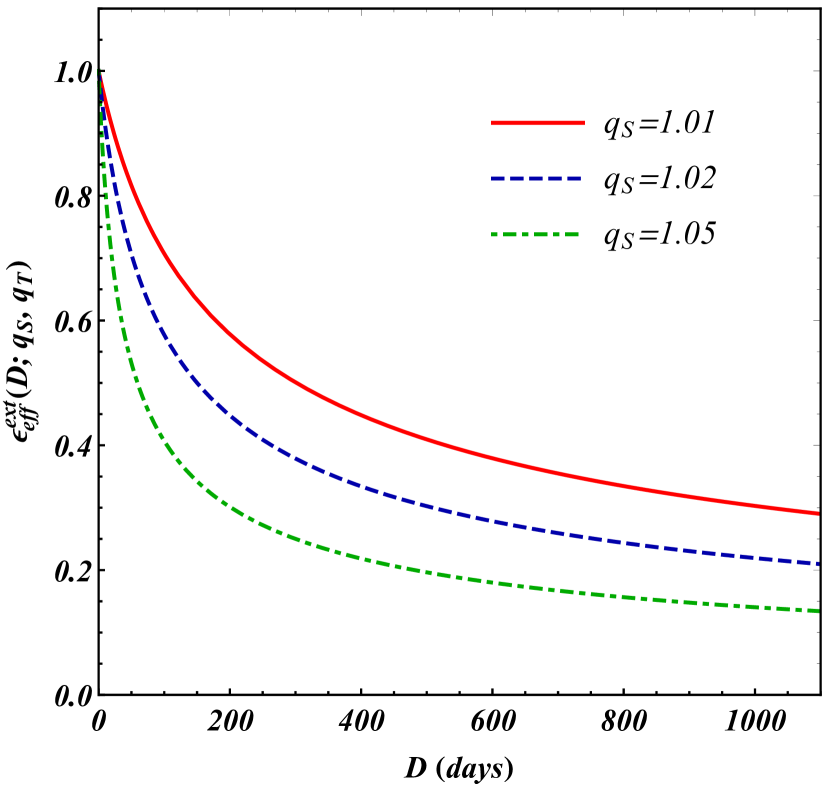
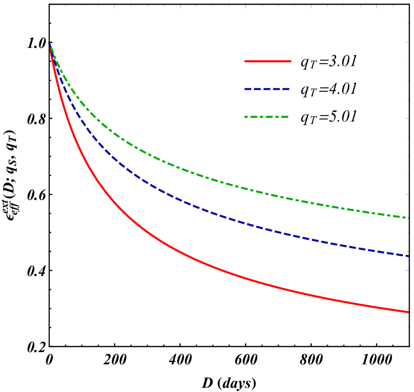
Eq. (16) is the first main result of our paper. To further explore the result, variation of the factor $\epsilon_{\text{eff}}^{\text{ext}}$ with delay is shown in Figs. (3) and (3). We can see that the factor monotonically decreases with delay and hence is suitable to describe the gradual decrease of indifference points in experimental observables. In section IV, we will consider a set of observed data to investigate the applicability of the model. However, before that we explore the mathematical implications of the model further.

Figure 2: Variation $\epsilon_{\text{eff}}^{\text{ext}}$ with $D$ for different $q_{\text{S}}$ values and for a fixed $q_{\text{T}}=3.01$.

Figure 3: Variation $\epsilon_{\text{eff}}^{\text{ext}}$ with $D$ for different $q_{\text{T}}$ values and for a fixed $q_{\text{S}}=1.01$.

III.5 Some comments about the model parameters

In this subsection, we aim to find out the significance of the parameters $q_{\text{S}}$ and $q_{\text{T}}$ that are to be determined by fitting experimental data. For this, we compute the average value of the variable $k_{\text{R}}$ that is given by,

$$\langle k_{\text{R}}\rangle=\left\langle\frac{k_{\text{T}}}{k_{\text{S}}}\right\rangle = \frac{\int_{0}^{\infty}dk_{\text{R}}k_{\text{R}}f(k_{\text{R}},k_{\text{A}})}{\int_{0}^{\infty}dk_{\text{R}}f(k_{\text{R}},k_{\text{A}})}$$ (20)

$$= \frac{\int_{0}^{\infty}dk_{\text{R}}k_{\text{R}}^{\alpha_{\text{T}}}(k_{\text{R}}+1)^{-\alpha_{\text{T}}-\alpha_{\text{S}}}}{\int_{0}^{\infty}dk_{\text{R}}k_{\text{R}}^{\alpha_{\text{T}}-1}(k_{\text{R}}+1)^{-\alpha_{\text{T}}-\alpha_{\text{S}}}}$$

$$= \frac{\alpha_{\text{T}}}{\alpha_{\text{S}}-1}=\frac{q_{\text{S}}-1}{(q_{\text{T}}-1)(2-q_{\text{S}})}~{}~{}~{}~{}~{}\text{(using Eq.~{}\ref{betafunc})}.$$

Since $k_{\text{R}}$ is a positive quantity, its average should be positive. This imposes a new constraint $q_{\text{S}}<2$ for Eq. (20) to be satisfied (since $q_{\text{S}},q_{\text{T}}>1$).

Eq. (20) is another important result obtained in this paper. As far as the experimental data are concerned, the ratio of model parameters obtained from the fitting of observed data will give us an idea of a sample’s average ratio of trait to state impulsivity. If the ratio $\alpha_{\text{T}}/(\alpha_{\text{S}}-1)$ exceeds 1, the average ratio of trait to state impulsivity of the participants is greater than 1. On the other hand, a sub-unity value of the ratio will imply a dominance of the state impulsivity. In our opinion, this ratio should be considered an important quantity in the study of mathematical models of delay discounting. We name this ratio the ‘inherence ratio’ $r_{\text{inh}}$ that is related to the relative value of inherent (trait) impulsivity with respect to the temporary (state) one. So, the inherence ratio is given by,

$$r_{\text{inh}}=\frac{\alpha_{\text{T}}}{\alpha_{\text{S}}-1}=\frac{q_{\text{S}}-1}{(q_{\text{T}}-1)(2-q_{\text{S}})}.$$ (21)

Since we have $1<q_{\text{S}}<2$ and $q_{\text{T}}>1$, $r_{\text{inh}}$ can be any positive real number. Consequently, our model can not predict if the trait characteristic will overshadow state or vice-versa and the values should depend on the sample being studied. This aspect will be explored in the next section with the help of observed datasets.

IV Data analysis using the E³M

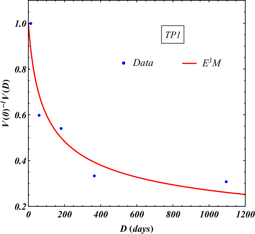
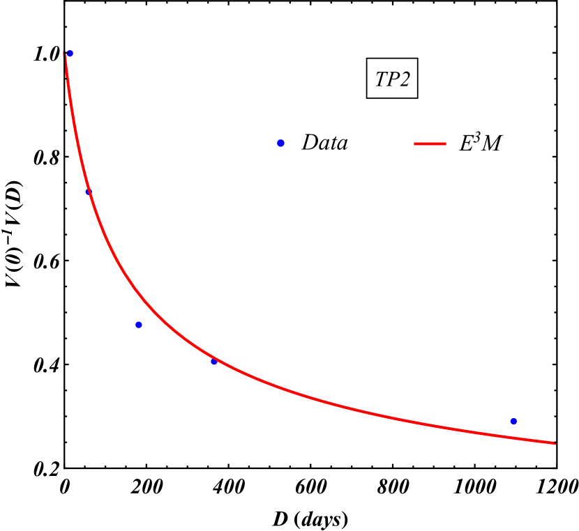
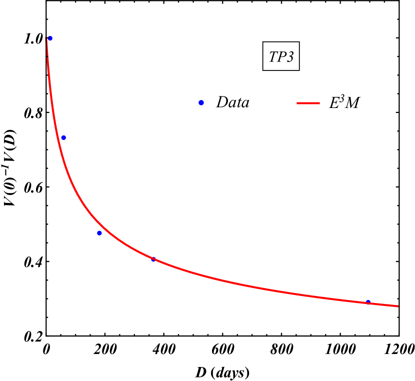
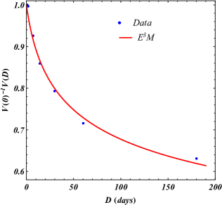
Methodology: We utilize our model in Eq. (16) to explain existing observed data for indifference points in delay discounting tasks. We consider eight datasets from three different studies (two longitudinal and one cross-sectional). Datasets are analyzed with the help of C++ codes utilizing the MINUIT package of the ROOT program Brun and Rademakers (1997). For visualization purposes and additional verification of results, the Mathematica software Wolfram Research, Inc., (2021) has been used.

Study	Reference	Sample size	Age (years)	Gender	Other criteria
1	Andrey P. Anokhin and Heath (2015)	560 (USA)	16-18	Female = 50.7%	1. No head trauma 2. No health conditions that restrict       physical movement
2	Escobar et al. (2023)	23 (Mexico)	18-22	Female = 65.2%	1. No substance use problems 2. No psychiatric diagnosis 3. No psychiatric medication
3	T.H. Mansouri (2020)	33 (USA)	19-48	Female = 57.6%	1. No smokers 2. No pregnant/breastfeeding participants 3. No medication that affects appetite 4. No allergies to study foods 5. No active effort to lose weight

Table 1: Descriptive statistics of the studies.

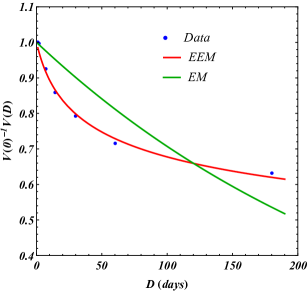
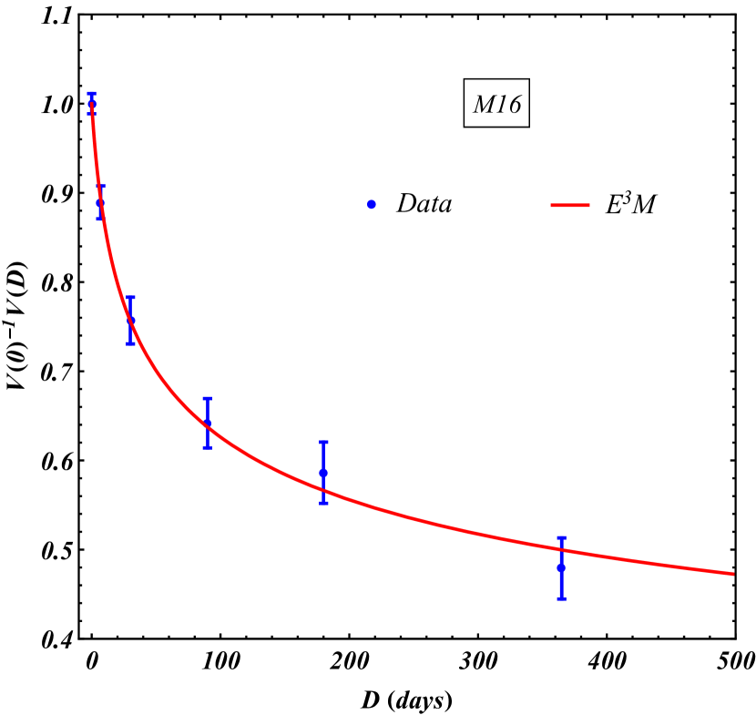
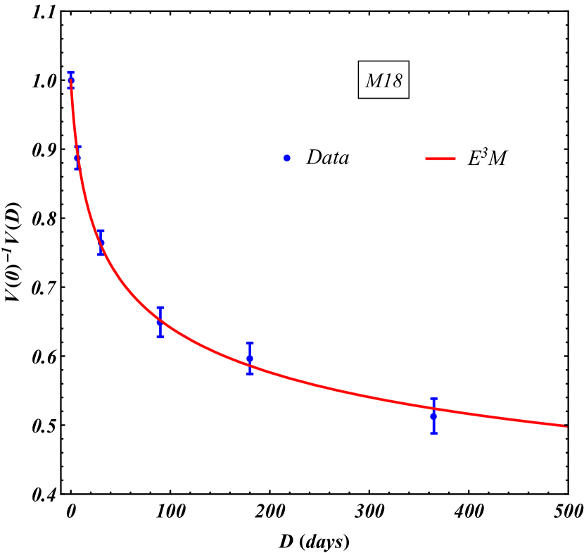
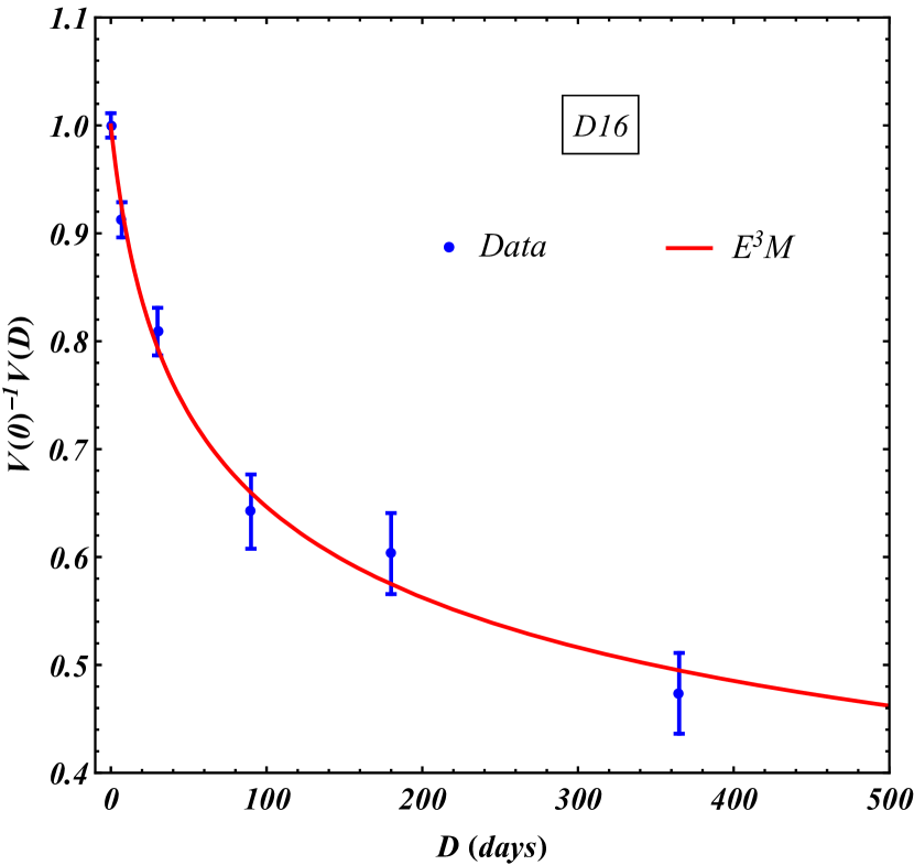
Findings: Considering the longitudinal data set associated with Refs. Andrey P. Anokhin and Heath (2015) (Study 1) and Escobar et al. (2023) (Study 2), we obtain Figs. (7)-(10). Additionally, we utilize the cross-sectional data set associated with Ref. T.H. Mansouri (2020) (Study 3) and obtain Fig. (11). The indifference points obtained from the experiments have been averaged over all the participants. Details of the studies yielding the datasets utilized in this paper are provided in Table 1. We observe that our model closely follows the data points in all these plots. Table 2 summarizes the results obtained from the description of the datasets using the E³M.

Study	Reference	Dataset	$q_{\text{T}}$	$q_{\text{S}}$	$r_{\text{inh}}$
1	Andrey P. Anokhin and Heath (2015)	Monozygotic, 16 yrs (M16)	$6.463\pm 0.816$	$1.113\pm 0.040$	$0.023\pm 0.003$
		Monozygotic, 18 yrs (M18)	$7.137\pm 0.705$	$1.134\pm 0.038$	$0.025\pm 0.003$
		Dizygotic, 16 yrs (D16)	$5.414\pm 0.800$	$1.057\pm 0.021$	$0.014\pm 0.002$
		Dizygotic, 18 yrs (D18)	$7.011\pm 0.624$	$1.120\pm 0.030$	$0.023\pm 0.002$
2	Escobar et al. (2023)	Time point 1 (TP1)	$3.525\pm 1.006$	$1.026\pm 0.024$	$0.011\pm 0.003$
		Time point 2 (TP2)	$3.113\pm 0.698$	$1.015\pm 0.009$	$0.007\pm 0.002$
		Time point 3 (TP3)	$4.044\pm 1.086$	$1.039\pm 0.038$	$0.013\pm 0.004$
3	T.H. Mansouri (2020)	-	$7.036\pm 0.261$	$1.091\pm 0.022$	$0.017\pm 0.001$

Table 2: A summary of the results obtained from description of existing datasets using the E³M.

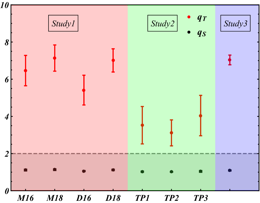
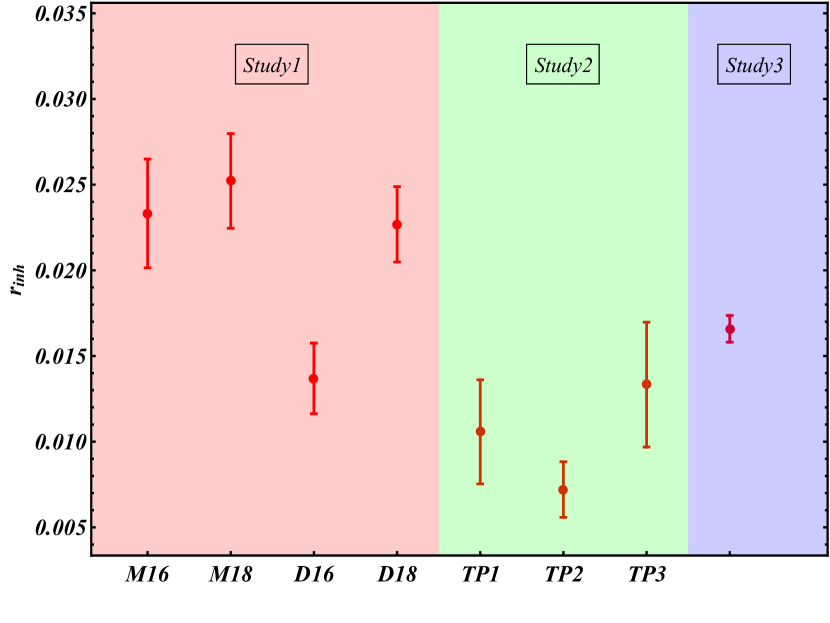
Figs. (13) and (13) graphically represent the parameter values obtained from the studies and the inherence ratio values. In these figures, Studies 1, 2, and 3 have been depicted by different shaded regions of red, green, and blue respectively. Interestingly, for these datasets, the additional constraint $q_{\text{S}}<2$, obtained from Eq. (20), is followed and $r_{\text{inh}}<1$. According to the E³M, this implies that the average relative value of state impulsivity with respect to trait impulsivity exceeds 1 for the analyzed samples, implying a dominance of the state characteristics.

From Fig. (13), it seems that the $q_{\text{S}}$ values (with error bars almost coinciding with the diameter of the data points used to represent the central values) are almost constant, but on closer inspection, we notice that the trend followed by $q_{\text{S}}$ is similar to that of $q_{\text{T}}$. Hence, the inherence ratios calculated from these parameter values also follow the same trend. In both longitudinal studies (1 and 2), a dip in the inherence ratio is observed. For Study 1, the dip is observed for the dizygotic twins at the age 16 (D16) and for Study 2, there is a dip in $r_{\text{inh}}$ value at time point 2 (TP2).

The dip in Study 1 is particularly of interest as the point is distinctly ‘separated’ from the other three considering even the error bars. As the inherence ratio signifies the average ratio of the trait to state impulsivity, the dip suggests a sudden increase in state impulsivity. Interestingly, in both studies, the $r_{\text{inh}}$ value recovers afterward. It will be interesting to investigate data from other longitudinal studies to find whether this trend is found.

We also observe that the $k_{1}$ parameter values obtained from the fitting of the same set of data (using Eq. (6)) is very close to (or overlapping with) the $r_{\text{inh}}$ values. Since the $k_{1}$ parameter can be explained as the average impulsivity of the sample T. Bhattacharyya and Pandey (2022) and $r_{\text{inh}}$ is related to the average ratio of trait to state impulsivity, the closeness of these two sets of values increases the reliability of our choice of the variable $k_{\text{R}}$ in terms of $k_{\text{T}}$ and $k_{\text{S}}$.

V Summary, conclusion and outlook

In this article, we propose an extension of the effective exponential model forwarded in Ref. T. Bhattacharyya and Pandey (2022). The present model, named the extended effective exponential model or E³M, considers bi-faceted impulsivity composed of trait and state parts. We assumed that trait and state impulsivity are represented by two positive, random variables. This is a sensible consideration given the fact that impulsivity does fluctuate in a social system from person to person. We find that with this consideration, the subjective value of a reward follows a power-law decay. However, unlike the EEM, this power-law decay is now dictated by a special function called the confluent hypergeometric function of the second kind.

The novelty of this article lies (a) in the superstatistics approach it takes and (b) in the fact that trait and state impulsivity are treated as two distinct variables. To our knowledge, this is the first such attempt to derive a mathematical model of delay discounting involving two distinct facets of impulsivity.

As we proceed with the mathematical analysis, an additional constraint like $q_{\text{S}}<2$ is discovered and a ratio called the inherence ratio represented by $r_{\text{inh}}$, which is related to the average ratio of the trait to state impulsivity of a sample has been proposed. Given the constraint $q_{\text{S}}<2$, we argue that the inherence ratio can be any positive number for observed datasets. Hence, no conclusions from the mathematical set-up could be drawn about the relative values of trait and state impulsivity. From the datasets analyzed in this paper, we observe that $r_{\text{inh}}<1$, implying a dominance of the state characteristics of the samples.

However, we consider only three different studies in this work, and more datasets need to be analyzed with the help of the E³M. It is also worth mentioning that the present article only studies temporal discounting. Similar studies may be carried out when other types of behaviour in effort discounting Mitchell (2004), probability discounting H. Rachlin and Cross (1991) and social discounting W. Białaszek (2019) are taken into account.

Another interesting formal development constitutes extending the E³M, considering more dimensions of impulsivity. There are some behavioural studies relying on a three-factor Kapitány-Fövény et al. (2020), or even the four-factor UPPS model S.P. Whiteside and Reynolds (2005) of impulsivity. The three-factor model posits cognitive impulsivity, behavioural impulsivity, and impatience/restlessness as the three facets, whereas the four-factor UPPS model considers the UPPS Impulsivity Scale comprising of four sub-scales: Urgency, (lack of) Premeditation, (lack of) Perseverance, and Sensation Seeking. We think that present method adapted in Section III may very well be extended to models accommodating multiple ($>$2) variables, but we reserve that work for the future.

To conclude, the approach adapted in the article is a generalized one involving random variables. It is, by no means, limited only to the studies of impulsivity and delay discounting. In fact, any system represented by random variables has benefited (e.g., physical systems like a thermal plasma) and will benefit from these lines of argument. So, we hope that more and more investigations in this direction will throw light on the applicability of the work in explaining systems represented by multi-faceted random variables.

Figures related to the analysis of experimental data

1. Study 1

Figure 4: Fitting of longitudinal data obtained from Ref. Andrey P. Anokhin and Heath (2015) for monozygotic twins at age 16 using the E³M: $q_{\text{S}}=1.113\pm 0.040,~{}q_{\text{T}}=6.463\pm 0.816$.

Figure 5: Fitting of longitudinal data obtained from Ref. Andrey P. Anokhin and Heath (2015) for monozygotic twins at age 18 using the E³M: $q_{\text{S}}=1.134\pm 0.038,~{}q_{\text{T}}=7.137\pm 0.705$.

Figure 6: Fitting of longitudinal data obtained from Ref. Andrey P. Anokhin and Heath (2015) for dizygotic twins at age 16 using the E³M: $q_{\text{S}}=1.057\pm 0.021,~{}q_{\text{T}}=5.414\pm 0.800$.

Figure 7: Fitting of longitudinal data obtained from Ref. Andrey P. Anokhin and Heath (2015) for dizygotic twins at age 18 using the E³M: $q_{\text{S}}=1.120\pm 0.030,~{}q_{\text{T}}=7.011\pm 0.624$.

2. Study 2

Figure 8: Fitting of longitudinal data obtained from Ref. Escobar et al. (2023) at time point 1 using the E³M: $q_{\text{S}}=1.026\pm 0.024,~{}q_{\text{T}}=3.525\pm 1.006$.

Figure 9: Fitting of longitudinal data obtained from Ref. Escobar et al. (2023) at time point 2 using the E³M: $q_{\text{S}}=1.015\pm 0.009,~{}q_{\text{T}}=3.113\pm 0.698$.

Figure 10: Fitting of longitudinal data obtained from Ref. Escobar et al. (2023) at time point 3 using the E³M: $q_{\text{S}}=1.039\pm 0.038~{}q_{\text{T}}=4.044\pm 1.086$.

3. Study 3

Figure 11: Fitting of observed data obtained from Ref. T.H. Mansouri (2020) using the E³M: $q_{\text{S}}=1.091\pm 0.022,~{}q_{\text{T}}=7.036\pm 0.261$.

4. Comparison of results obtained from all the datasets used in the paper

Figure 12: Values of $q_{\text{S}}$ and $q_{\text{T}}$ obtained by fitting observed data utilizing the E³M.

Figure 13: Values of the inherence ratio $r_{\text{inh}}$ calculated from different studies.

References

- Abramowitz and Stegun (1972a) Abramowitz, M. and Stegun, I., editors (1972a). Beta Function. §6.2, p. 258. in Handbook of Mathematical Functions with Formulas, Graphs, and Mathematical Tables. Dover, 10th edition.
- Abramowitz and Stegun (1972b) Abramowitz, M. and Stegun, I., editors (1972b). Confluent Hypergeometric Functions. Ch. 13, pp. 503-515. in Handbook of Mathematical Functions with Formulas, Graphs, and Mathematical Tables. Dover, 10th edition.
- Abramowitz and Stegun (1972c) Abramowitz, M. and Stegun, I., editors (1972c). Gamma (Factorial) Function. §6.1 in Handbook of Mathematical Functions with Formulas, Graphs, and Mathematical Tables. Dover, 10th edition.
- Andrey P. Anokhin and Heath (2015) Andrey P. Anokhin, Julia D. Grant, R. C. M. and Heath, A. C. (2015). The genetics of impulsivity: Evidence for the heritability of delay discounting. Biological Psychiatry, 77(10):887–894.
- Antons and Brand (2018) Antons, S. and Brand, M. (2018). Trait and state impulsivity in males with tendency towards internet-pornography-use disorder. Addictive Behavior, 79:171–177.
- Beck and Cohen (2003) Beck, C. and Cohen, E. (2003). Superstatistics. Physica A, 322:267–275.
- Brun and Rademakers (1997) Brun, R. and Rademakers, F. (1997). Root - an object-oriented data analysis framework, proceedings aihenp’96 workshop, lausanne, sep. 1996. Nuclear Instruments and Methods in Physics Research A, 389:81–86.
- Budini (2015) Budini, A. (2015). Extended -gaussian and -exponential distributions from gamma random variables. Physical Review E, 91(052113):1–11.
- Cajueiro (2006) Cajueiro, D. (2006). A note on the relevance of the -exponential function in the context of intertemporal choices. Physica A, 364:385–388.
- Critchfield and Kollins (2001) Critchfield, T. and Kollins, S. (2001). Temporal discounting: Basic research and the analysis of socially important behavior. Journal of Applied Behavior Analysis, 34(1):101–122.
- Escobar et al. (2023) Escobar, G. G., Morales-Chainé, S., Haynes, J. M., Santoyo, C., and Mitchell, S. H. (2023). Moderate stability among delay, probability, and effort discounting in humans. The Psychological Record, pages 1–14.
- Griffin and Trull (2021) Griffin, S. and Trull, T. (2021). Alcohol use in daily life: Examining the role of trait and state impulsivity facets. Psychological Addictive Behavior, 35(2):199–207.
- H. Rachlin and Cross (1991) H. Rachlin, A. R. and Cross, D. (1991). Subjective probability and delay. Journal of the Experimental Analysis of Behavior, 55(2):233–244.
- I.M.P. Oller and Martinez (2021) I.M.P. Oller, S. R. and Martinez, M. (2021). Discount models in intertemporal choice: an empirical analysis. European Journal of Management and Business Economics, 30(1):72–91.
- Ishii and Eisen (2018) Ishii, K. and Eisen, C. (2018). Cultural similarities and differences in social discounting: The mediating role of harmony-seeking. Frontiers in Psychology, 9:1426.
- Joel Myerson (1995) Joel Myerson, L. G. (1995). Discounting of delayed rewards: models of individual choice. Journal of The Experimental Analysis of Behavior, 64:263–276.
- Kapitány-Fövény et al. (2020) Kapitány-Fövény, M., Urbán, R., Varga, G., Potenza, M. N., Griffiths, M. D., Szeleky, A., Paksi, B., Kun, B., Farkas, J., Kökönyei, G., and Demetrovics, Z. (2020). The 21-item barratt impulsiveness scale revised (bis-r-21): An alternative three-factor model. Journal of Behavioral Addictions, 9(2):225–246.
- Lempert and Pizzagalli (2010) Lempert, K. and Pizzagalli, D. (2010). Delay discounting and future-directed thinking in anhedonic individuals. Journal of Behavior Therapy and Experimental Psychiatry, 41:258–264.
- Mazur (1987) Mazur, J. (1987). The effect of delay and of intervening events on reinforcement value, volume 5, chapter An adjusting procedure for studying delayed reinforcement, pages 55–73. Lawrence Erlbaum Associates, Inc.
- McKerchar et al. (2009) McKerchar, T. L., Green, L., Myerson, J., Pickford, T. S., Hill, J. C., and Stout, S. C. (2009). A comparison of four models of delay discounting in humans. Behavioural Processes, 81(2):256–259.
- Mitchell (2004) Mitchell, S. (2004). Effects of short-term nicotine deprivation on decision-making: Delay, uncertainty and effort discounting. Nicotine & Tobacco Research, 6(5):819–828.
- Odum (2011) Odum, A. (2011). Delay discounting: I’m a k, you’re a k. Journal of the Experimental Analysis of Behavior, 96(3):427–439.
- Rachlin (2006) Rachlin, H. (2006). Notes on discounting. Journal of The Experimental Analysis of Behavior, 85:425–435.
- Rachlin and Jones (2008) Rachlin, H. and Jones, B. (2008). Social discounting and delay discounting. Journal of Behavioral Decision Making, 21:29–43.
- R.V. Hogg and Craig (2019) R.V. Hogg, J. M. and Craig, A. (2019). Introduction to Mathematical Statistics. Pearson Education.
- Samuelson (1937) Samuelson, P. (1937). A note on measurement of utility. The Review of Economic Studies, 4:155–161.
- S.P. Whiteside and Reynolds (2005) S.P. Whiteside, D.R. Lynam, J. M. and Reynolds, S. (2005). Validation of the upps impulsive behaviour scale: a four-factor model of impulsivity. European Journal of Personality, 19:559–574.
- Stegall et al. (2019) Stegall, S., Collette, T., Kinjo, T., Takahashi, T., and Romanowich, P. (2019). Quantitative cross-cultural similarities and differences in social discounting for gains and losses. Frontiers in Public Health, 7:297.
- T. Bhattacharyya and Pandey (2022) T. Bhattacharyya, S. S. and Pandey, R. (2022). A tsallis-like effective exponential delay discounting model and its implications. Physica A, 603(127836):1–8.
- Takahashi (2007) Takahashi, T. (2007). A comparison of intertemporal choices for oneself versus someone else based on tsallis’ statistics. Physica A, 385:637–644.
- Takahashi (2010) Takahashi, T. (2010). A social discounting model based on tsallis’ statistics. Physica A, 389:3600–3603.
- Takahashi et al. (2012) Takahashi, T., Nishinaka, H., Makino, T., Han, R., and Fukui, H. (2012). An experimental comparison of quantum decision theoretical models of intertemporal choice for gain and loss. Journal of Quantum Information Science, 2:119–122.
- T.H. Mansouri (2020) T.H. Mansouri, A.K. Crandall, J. T. (2020). The effect of repeated episodic future thinking on the relative reinforcing value of snack food. Journal of Health Psychology, 26(13):2402–2413.
- Tsallis (1988) Tsallis, C. (1988). Possible generalization of boltzmann-gibbs statistics. Journal of Statistical Physics, 52:479–487.
- Tversky and Kahneman (1986) Tversky, A. and Kahneman, D. (1986). Rational choice and the framing of decisions. The Journal of Business, 59(4):S251–S278.
- W. Białaszek (2019) W. Białaszek, P. Ostaszewski, L. G. . J. M. (2019). On four types of devaluation of outcomes due to their costs: Delay, probability, effort, and social discounting. The Psychological Record, 69:415–424.
- West and Grigolini (2010) West, B. and Grigolini, P. (2010). A psychophysical model of decision making. Physica A, 389:3580–3587.
- Wilk and Wĺodarczyk (2000) Wilk, G. and Wĺodarczyk, Z. (2000). Interpretation of the nonextensivity parameter in some applications of tsallis statistics and lévy distributions. Physical Review Letters, 84:2770–2773.
- Wingrove and Bond (1997) Wingrove, J. and Bond, A. (1997). Impulsivity: A state as well as trait variable. does mood awareness explain low correlations between trait and behavioural measures of impulsivity? Personality and Individual Differences, 22(3):333–339.
- Wolfram Research, Inc., (2021) Wolfram Research, Inc., (2021). Mathematica, Version 13. Champaign, IL.