Batches Stabilize the Minimum Norm Risk in High Dimensional Overparameterized Linear Regression

Abstract

Learning algorithms that divide the data into batches are prevalent in many machine-learning applications, typically offering useful trade-offs between computational efficiency and performance. In this paper, we examine the benefits of batch-partitioning through the lens of a minimum-norm overparameterized linear regression model with isotropic Gaussian features. We suggest a natural small-batch version of the minimum-norm estimator, and derive an upper bound on its quadratic risk, showing it is inversely proportional to the noise level as well as to the overparameterization ratio, for the optimal choice of batch size. In contrast to minimum-norm, our estimator admits a stable risk behavior that is monotonically increasing in the overparameterization ratio, eliminating both the blowup at the interpolation point and the double-descent phenomenon. Interestingly, we observe that this implicit regularization offered by the batch partition is partially explained by feature overlap between the batches. Our bound is derived via a novel combination of techniques, in particular normal approximation in the Wasserstein metric of noisy projections over random subspaces.

1 Introduction

Batch-based algorithms are used in various machine-learning problems. Particularly, partition into batches is natural in distributed settings, where data is either collected in batches by remote sensors who can send a small number of bits to a central server, or collected locally but offloaded to multiple remote workers for computational savings, see e.g. [1, 2, 3, 4, 5, 6, 7, 8, 9, 10]. Learning in batches is also employed in centralized settings; this is often done to reduce computational load, but is also known (usually empirically) to sometimes achieve better convergence, generalization, and stability, see e.g., [4, 11, 12]. One of the most basic and prevalent learning tasks is linear regression, which has been extensively studied in both centralized and distributed settings. Linear regression is of particular contemporary interest in the overparameterized regime, where the number of parameters exceeds the number of samples. In this regime there are infinitely many interpolators, and a common regularization method is to pick the minimum norm (min-norm) solution, i.e., the interpolator whose $\ell_{2}$ norm is minimal. However, this method requires inverting a matrix whose dimensions are the number of samples, a task that can be computationally costly and also result in a non-stable risk, growing unbounded close to the interpolation point [13, 14]. Performing linear regression separately in batches and combining the solutions (usually by averaging) can help with the computational aspects, and has been studied before mainly for large (linear in the number of samples) batches [7, 8, 9, 10]. However, such solutions break down and cannot control the risk for sublinear batch size; they also shed no light on the performance benefits heuristically known to be offered by small batches. Can the min-norm solution benefit more from small batch partitioning? We answer this question in the affirmative, by suggesting a simple and natural min-norm-based small-batch regression algorithm, and showing it stabilizes the min-norm risk. We discuss the ramifications of our result in several settings.

1.1 Our Contribution

We consider a linear model with isotropic features, in the overparameterized regime with $n$ data samples and $p>n$ parameters, where the $n\times p$ feature matrix is i.i.d. Gaussian. The risk attained by min-norm in this setting and related ones was previously analyzed in [14]. Here, we suggest the following small batch variation of min-norm. First, the data is partitioned into small disjoint batches of equal size $b$, and a simple min-norm estimator is computed separately for each batch. Then, the resulting $\frac{n}{b}$ weak estimators are pooled together to form a new $\frac{n}{b}\times p$ feature matrix for a modified “linear” model, with suitably weighted modified samples. The modified model is not truly linear, since both the new features and noise depend on the parameter. Finally, a min-norm estimator is computed in this new setting, yielding our suggested batch minimum norm (batch-min-norm) estimator. Note that while the modified model is far more overparameterized than the original model (by a factor of $b$), its features are now favorably correlated / better aligned with the underlying parameters. We shall see that this trade-off can be beneficial.

To that end, we derive an upper bound on the risk obtained by our estimator, in the limit of $n,p\to\infty$ with a fixed overparameterization ratio $\gamma=p/n$, as a function of the $\mathsf{SNR}$. Our bound is compared to simulations and is demonstrated to be quite tight. We then analytically find the batch size minimizing the bound, and show that it is inversely proportional to both $\gamma$ and $\mathsf{SNR}$; in particular, there is a low-$\mathsf{SNR}$ threshold point below which increasing the batch size (after taking $n,p\to\infty$) is always beneficial (albeit at very low $\mathsf{SNR}$ we can do worse that the null solution), see Figure 1. Unlike min-norm, and similarly to optimally-tuned ridge regression [15], the risk attained by batch-min-norm is generally stable; it is monotonically increasing in $\gamma$, does not explode near the interpolation point $\gamma=1$, and does not exhibit a double descent phenomenon [14] (all this assuming $\mathsf{SNR}$ $\geq 1$, see Figure 2). It is (trivially) always at least as good (and often much better) than min-norm. Another interesting observation is that the batch algorithm exactly coincides with the regular min-norm algorithm for any batch size, whenever the feature matrix has orthogonal rows. Thus, somewhat intriguingly, the reason that batches are useful can be partially attributed to the fact that feature vectors are slightly linearly dependent between batches, i.e., there is small overlap between the subspaces spanned by the batches. From a technical perspective, as we shall later see, this overlap implicitly regularizes the noise amplification suffered by the standard min-norm.

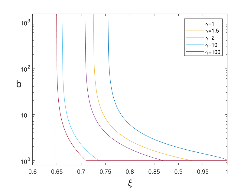
(a)

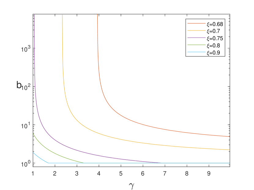
(b)

Figure 1: Optimal batch size vs. (a) normalized signal-to-noise ratio $\xi=\frac{\mathsf{SNR}}{1+\mathsf{SNR}}$, and (b) overparametrization ratio $\gamma$. When $\xi<0.6478$, the optimal batch size $b\rightarrow\infty$, for any $\gamma>1$.

The derivation of the upper bound is the main technical contribution of the paper. The main difficulty lies in the second step of the algorithm, namely analyzing the min-norm with the feature matrix comprised of per-batch min-norm estimators. Note that this step is no longer under a standard linear model; in particular, the new feature matrix and the corresponding noise vector depend on the parameters, and the noise vector also depends on the feature matrix, in a generally non-linear way. This poses a significant technical barrier requiring the use of several nontrivial mathematical tools. To compute the bias of the algorithm, we first write it as a recursive perturbed-projection onto a random per-batch subspace, drawn from the Haar measure on the Stiefel manifold. We show that the statistics of these projections are asymptotically close in the Wasserstein metric to i.i.d. Gaussian vectors, a fact that allows us to obtain a recursive expression for the bias as batches are being added, with a suitable control over the error term. We then translate this recursion into a certain differential equation, whose solution yields the asymptotic expression for the bias. To bound the variance of the algorithm, we show that it converges to a variance of a Gaussian mixture with $\chi^{2}$-distributed weights, projected onto the row-space of a large Wishart matrix.

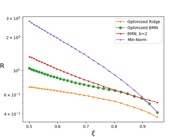
(a)

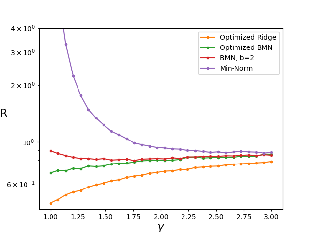
(b)

Figure 2: Risk of batch-min-norm with optimal batch size vs. (a) normalized signal-to-noise ratio $\xi=\frac{\mathsf{SNR}}{1+\mathsf{SNR}}$, with $\gamma=1.4$, and (b) overparametrization ratio $\gamma$ with $\xi=0.7$. Optimized ridge is ridge regression with the optimal regularization parameter.

1.2 Ramifications

Distributed linear regression. In this setting, the goal is usually to offload the regression task from the main server by distributing it between multiple workers; the main server then merges the estimates given by the workers. This merging is typically done by simple averaging, e.g., [1, 2, 7, 9]. The number of workers is typically large but fixed, hence the batch size is linear in the sample size. The regime of sublinear batch sizes is less explored in the literature, perhaps due to practical reasons. When the batch size is sublinear, the server-averaging approach breaks down since its risk is trivially dominated by the per-batch bias, and hence it attains the null risk asymptotically. In contrast, our algorithm projects the modified observations onto the subspace spanned by the entire collection of weak estimators. Hence, the resulting estimator is much less biased than each weak estimator separately. Therefore, our algorithm is far superior to server-averaging for fixed batch size. Numerical results indicate that this is also true in the general sublinear regime.

Linear regression under real-time communication constraints. Consider a low-complexity sensor sequentially viewing samples (feature vectors and observations). The sensor cannot collect all the samples and perform the regression task, hence it offloads the task to a remote server, with which it can communicate over a rate-limited channel. Due to the communication constraint, the sensor cannot send all of its samples to the server. Our algorithm gives a natural solution: choose a batch size $b$ large enough such that sending $(p+1)/b$ samples per unit of time becomes possible, and send the min-norm solution of each batch to the server, who in turn will run the second step of the algorithm. Our bounds show how the risk behaves as a function of $b$. For reasons already mentioned, this algorithm is far better than simple solutions such as averaging or trivially sending one in $b$ samples. We note that the general topic of statistical inference under communication constraints has been extensively explored (see e.g. [16, 17, 18, 19, 20, 21, 22] but typically for a fixed parameter dimension, which does not cover the overparameterized setting we consider here.

Mini-batch learning, High-dimensional overparameterized linear regression is known to sometimes serve as a reasonable proxy (via linearization) to more complex settings such as deep neural networks [23, 24, 25, 26, 27]. Furthermore, min-norm is equivalent to full Gradient Descent (GD) in linear regression, and even exhibits similar behavior observed when using GD in complex models, e.g. the double-descent [14]. Learning using small batches, e.g. mini-batch SGD, is a common approach that originated from computational considerations[28, 11], but was also observed to improve generalization [29, 30, 31, 32, 33, 34]. There is hence clear impetus to study the impact of small batches on min-norm-flavor algorithms in the linear regression setting. Indeed, mini-batch SGD for linear regression has been recently studied in [35], who gave closed-form solutions for the risk in terms of Volterra integral equations (see also [36] for a more general setting using mean field theory). In particular, and in contrast to a practically observed phenomenon in deep networks, [35] showed that the linear regression risk of mini-batch SGD does not depend on the batch size $b$ as long as $b\ll n^{1/5}$. Our batch-min-norm algorithm, while clearly not equivalent to mini-batch SGD in the linear regression setting, does exhibit the small-batch gain phenomenon, and hence could perhaps nevertheless shed some light on similar effects empirically observed in larger models. In particular, the batch regularization effect we observe can be traced back to a data “overlap” between the batches, and it is interesting to explore whether this effect manifests itself in other settings. Moreover, from a high-level perspective, our algorithm “summarizes” each batch to create a “representative sample”, and then trains again via GD only on these representative samples. It is interesting to explore whether this approach can be rigorously generalized to more complex models.

2 Preliminaries

2.1 Notation

We write $x,\boldsymbol{y}$, and $A$ for scalars, vectors and matrices, respectively. Vectors can be either row or column, as clear from context. We use $X$, $\boldsymbol{X}$ and $\boldsymbol{A}$ to denote random variables, random vectors, and random matrices, respectively. We write $\|A\|_{2}$ and sometimes $\|A\|$ for the $\ell_{2}$ norm of the matrix $A$, and $\|A\|_{op}$, $\|A\|_{F}$ for the operator and Frobenius norms of $A$, respectively. For a real-valued p.s.d. matrix $A$, we write $\lambda_{i}(A)$ to denote the $i$-th largest eigenvalue of $A$, and $\lambda_{\text{min}}(A)$, $\lambda_{\text{max}}(A)$ for the minimal and maximal eigenvalues of $A$, respectively. We say that $b$ orthonormal random column vectors $\boldsymbol{U}_{1},\cdots,\boldsymbol{U}_{b}\in\mathbb{R}^{n}$ are uniform or uniformly drawn, if the matrix $\boldsymbol{U}=[\boldsymbol{U}_{1},\cdots,\boldsymbol{U}_{b}]$ is drawn from the Haar measure on the Stiefel manifold $\mathbb{V}_{b}(\mathbb{R}^{n})\triangleq\{\boldsymbol{A}\in\mathbb{R}^{b\times n}:\boldsymbol{A}\boldsymbol{A}^{T}=\boldsymbol{I}_{b}\}$, where $\boldsymbol{I}_{b}$ is the $b\times b$ identity matrix. We sometimes drop the subscript and write $\boldsymbol{I}$, when the dimension is clear from context. We write $X_{n}\overset{P}{\longrightarrow}X$ (resp. $X_{n}\overset{\text{a.s}}{\longrightarrow}X$) to indicate that the sequence $X_{1},X_{2},\cdots$ of random variables converges to the random variable $X$ in probability (resp. almost surely (a.s.)). Similar notation for (finite-dim) random vectors / matrices means convergences of all entries.

2.2 Wasserstein Distance

The $p$-Wasserstein distance between two probability measures $\mu$ and $\nu$ on $\mathbb{R}^{n}$ is

$$\mathcal{W}_{p}(\mu,\nu)\triangleq\left(\,\inf\mathbb{E}\|\boldsymbol{X}-\boldsymbol{Y}\|_{2}^{p}\,\right)^{\frac{1}{p}},$$ (1)

where the infimum is taken over all random vector pairs $(\boldsymbol{X},\boldsymbol{Y})$ with marginals $\boldsymbol{X}\sim\mu$ and $\boldsymbol{Y}\sim\nu$. With a slight abuse of notations, we write $\mathcal{W}_{p}(\boldsymbol{X},\boldsymbol{Y})$ to indicate the $p$-Wasserstein distance between the corresponding probability measures of $\boldsymbol{X}$ and $\boldsymbol{Y}$. Throughout this paper we say Wasserstein distance to mean the $1$-Wasserstein distance $\mathcal{W}_{1}(\mu,\nu)$, unless explicitly mentioned otherwise. The following theorem is the well-known dual representation of the $1$-Wasserstein distance.

Theorem 1 ($\mathcal{W}_{1}$ duality ([37])).

For any two probability measures $\mu$ and $\nu$ over $\mathbb{R}^{n}$, it holds that

$$\mathcal{W}_{1}(\mu,\nu)=\sup\,\mathbb{E}f(\boldsymbol{X})-\mathbb{E}f(\boldsymbol{Y}),$$ (2)

where $\boldsymbol{X}\sim\mu$, $\boldsymbol{Y}\sim\nu$, and the supremum is taken over all $1$-Lipschitz functions $f:\mathbb{R}^{n}\to\mathbb{R}$.

It was previously shown in [38] that low-rank projection of uniformly random orthonormal matrix is close to Gaussian in Wasserstein distance. This result is summarized in the following theorem.

Theorem 2 (Theorem 11 in [38]).

Let $B_{1},\cdots,B_{k}$ be linearly independent $p\times p$ matrices (i.e. the only linear combination of them which is equal to the zero matrix has all coefficients equal to zero) over $\mathbb{R}$ such that $\operatorname{Tr}{(B_{i}B^{T}_{i})}=p$ for $i=1,\cdots,k$. Define $b_{ij}\triangleq\operatorname{Tr}{(B_{i}B^{T}_{j})}$, let $\boldsymbol{G}=[G_{1},...,G_{k}]$ be a random vector whose components have Gaussian distribution, with zero mean and covariance matrix $C\triangleq\frac{1}{p}(b_{ij})$ and let $\boldsymbol{U}$ be a uniformly random orthogonal matrix. Then, for

$$\boldsymbol{S}\triangleq\left[\operatorname{Tr}{(B_{1}\boldsymbol{U})},\operatorname{Tr}{(B_{2}\boldsymbol{U})},\cdots,\operatorname{Tr}{(B_{k}\boldsymbol{U})}\right]\in\mathbb{R}^{k},$$ (3)

and any $p\geq 2$ we have

$$\mathcal{W}_{1}(\boldsymbol{S},\boldsymbol{G})\leq\frac{k\sqrt{2\|C\|_{\textrm{op}}}}{p-1}.$$ (4)

The Wasserstein distance plays a key role in our proofs, mainly due to the following facts. First, our batch-min-norm algorithm performs projections onto small random subspaces, and Wasserstein distance can be used to quantify how far these are from projections onto i.i.d. Gaussian vectors using Theorem 2. Second, closeness in Wasserstein distance implies change-of-measure inequalities for expectations of Lipschitz functions via the Kantorovich-Rubinstein duality theorem (Theorem 1), which allows us to compute expectations in the more tractable Gaussian domain with proper error control. For further details on the properties of Wasserstein distance, see Appendix A.1.

3 Problem setup

Let $\boldsymbol{Y}=(Y_{1},\cdots,Y_{n})^{T}$ be a data samples vector obtained from the linear model

$$\boldsymbol{Y}=\boldsymbol{X}\boldsymbol{\beta}+\boldsymbol{W}$$ (5)

where $\boldsymbol{\beta}\in\mathbb{R}^{p}$ is a vector of unknown parameters, $\boldsymbol{X}\in\mathbb{R}^{n\times p}$ is a given feature matrix with i.i.d. standard Gaussian entries, and $\boldsymbol{W}\in\mathbb{R}^{n}$ is a noise vector independent of $\boldsymbol{X}$ with i.i.d. $\mathcal{N}(0,\sigma^{2})$ entries. We write

$$\|\boldsymbol{\beta}\|_{2}=r,$$ (6)

to denote the norm of $\boldsymbol{\beta}$, which is assumed unknown unless otherwise stated. Define the overparametrization ratio $\gamma\triangleq\frac{p}{n}$. When $\gamma>1$ we call the problem overparameterized and when $\gamma<1$ we say it is underparametrized. An estimator $\hat{\boldsymbol{\beta}}=\hat{\boldsymbol{\beta}}(\boldsymbol{Y},\boldsymbol{X})$ for $\boldsymbol{\beta}$ from the samples and features is a mapping $\hat{\boldsymbol{\beta}}:\mathbb{R}^{n}\times\mathbb{R}^{n\times p}\to\mathbb{R}^{p}$. We measure the performance of an estimator via the quadratic (normalized) risk $R(\hat{\boldsymbol{\beta}})$ it attains:

$$R(\hat{\boldsymbol{\beta}})\triangleq\frac{1}{r^{2}}\,\mathbb{E}\|\hat{\boldsymbol{\beta}}(\boldsymbol{Y},\boldsymbol{X})-\boldsymbol{\beta}\|^{2}.$$ (7)

Note that while $R(\hat{\boldsymbol{\beta}})$ is the parameter estimation risk, it is also equal in this case (up to a constant) to the associated prediction risk, namely the mean-squared prediction error $\mathbb{E}\|\mathbf{x}^{T}\hat{\boldsymbol{\beta}}-\mathbf{x}^{T}\boldsymbol{\beta}\|^{2}$ when using $\hat{\boldsymbol{\beta}}$ to estimate the response to a new i.i.d. feature vector $\mathbf{x}$.

3.1 Minimum-Norm Estimation

In the overparametrized case $\gamma>1$, there is an infinite number of solutions to the linear model $\boldsymbol{X}\boldsymbol{\beta}=\boldsymbol{y}$, and in order to choose one we need to impose some regularization. A common choice is the $\ell_{2}$-norm regularization, which yields the min-norm estimator, defined as

$$\hat{\boldsymbol{\beta}}_{\mathrm{MN}}\triangleq\operatorname*{\arg\!\min}\|\boldsymbol{\beta}\|_{2}^{2},\text{ s.t. }\boldsymbol{X}\boldsymbol{\beta}=\boldsymbol{y},$$ (8)

and explicitly given by

$$\hat{\boldsymbol{\beta}}_{\mathrm{MN}}=\boldsymbol{X}^{T}(\boldsymbol{X}\boldsymbol{X}^{T})^{-1}\boldsymbol{y}.$$ (9)

The risk of the min-norm estimator is then

$$R(\hat{\boldsymbol{\beta}}_{\mathrm{MN}})=\left(1-\frac{1}{r^{2}}\mathbb{E}\left\|\boldsymbol{L}\boldsymbol{\beta}\right\|^{2}\right)+\frac{1}{r^{2}}\mathbb{E}\left[\boldsymbol{W}^{T}(\boldsymbol{X}\boldsymbol{X}^{T})^{-1}\boldsymbol{W}\right],$$ (10)

where $\boldsymbol{L}=\boldsymbol{X}^{T}(\boldsymbol{X}\boldsymbol{X}^{T})^{-1}\boldsymbol{X}$ is the orthogonal projection onto the row space of $\boldsymbol{X}$, and we used the fact that the matrix $\boldsymbol{X}$ is orthogonal to its null space $\boldsymbol{I}-\boldsymbol{L}$. The first term in the above is the (normalized) bias of the estimator, which represents the part of $\boldsymbol{\beta}$ that is not captured in the subspace spanned by $\boldsymbol{X}$. The second term is the (normalized) variance of the estimator. As previously shown in [14], the asymptotic risk of the min-norm estimator under the above model is

$$\lim_{p\rightarrow\infty}R(\hat{\boldsymbol{\beta}}_{\mathrm{MN}})=1-\gamma^{-1}+\frac{1-\xi}{\xi}\cdot\frac{1}{\gamma-1}.$$ (11)

where

$$\xi\triangleq\frac{r^{2}}{r^{2}+\sigma^{2}}=\frac{\mathsf{SNR}}{1+\mathsf{SNR}},$$ (12)

is the normalized $\mathsf{SNR}$, with $\mathsf{SNR}\triangleq r^{2}/\sigma^{2}$. The parameter $\xi$ is also known as the Wiener coefficient.

4 Batch Minimum-Norm Estimation

We proceed to suggest and study a natural batch version of the min-norm estimator. Let us divide the samples $\boldsymbol{Y}$ to $n/b$ batches of some fixed size $b$, and denote by $\boldsymbol{Y}_{j}\in\mathbb{R}^{b}$ the $j$th batch. From each batch $\boldsymbol{Y}_{j}$ we can obtain a min-norm estimate of $\boldsymbol{\beta}$, given by

$$\hat{\boldsymbol{\beta}}_{j}\triangleq\boldsymbol{X}_{j}^{T}(\boldsymbol{X}_{j}\boldsymbol{X}_{j}^{T})^{-1}\boldsymbol{Y}_{j},\quad j=1,\cdots,n/b,$$ (13)

where $\boldsymbol{X}_{j}$ are the feature vectors that correspond to $\boldsymbol{Y}_{j}$. We now have $n/b$ weak estimators for $\boldsymbol{\beta}$, each predicting only a tiny portion of $\boldsymbol{\beta}$’s energy. However, these estimators are clearly better correlated with $\boldsymbol{\beta}$ compared to random features. Hence, it makes sense to think of each $\hat{\boldsymbol{\beta}}_{j}^{T}$ as a modified feature vector $\boldsymbol{x}^{\prime}_{j}$ that summarizes what was learned from batch $j$. Since each modified feature vector is a linear combination of its batch’s feature vectors, with coefficients $\boldsymbol{Y}_{j}^{T}\cdot(\boldsymbol{X}_{j}\boldsymbol{X}_{j}^{T})^{-1}$, we can construct the corresponding modified sample for batch $j$, given by

$$Y^{\prime}_{j}\triangleq\boldsymbol{Y}_{j}^{T}\cdot(\boldsymbol{X}_{j}\boldsymbol{X}_{j}^{T})^{-1}\boldsymbol{Y}_{j}=\hat{\boldsymbol{\beta}}_{j}^{T}\boldsymbol{\beta}+W^{\prime}_{j}=\boldsymbol{x}^{\prime}_{j}\boldsymbol{\beta}+W^{\prime}_{j},$$ (14)

where

$$W^{\prime}_{j}=\boldsymbol{Y}_{j}^{T}(\boldsymbol{X}_{j}\boldsymbol{X}_{j}^{T})^{-1}\boldsymbol{W}_{j},$$ (15)

is the corresponding modified noise.

We can now pool all these modified quantities to form a new model:

$$\boldsymbol{Y}^{\prime}=\boldsymbol{X}^{\prime}\boldsymbol{\beta}+\boldsymbol{W}^{\prime},$$ (16)

where the modified feature matrix $\boldsymbol{X}^{\prime}$ and modified noise vector $\boldsymbol{W}^{\prime}$ are given by

$$\boldsymbol{X}^{\prime} =\left[{\hat{\boldsymbol{\beta}}}_{1},\cdots,{\hat{\boldsymbol{\beta}}}_{n/b}\right]^{T}=\left[{\boldsymbol{x}^{\prime}}_{1}^{T},\cdots,{\boldsymbol{x}^{\prime}}_{n/b}^{T}\right]^{T},$$ (17)

$$\boldsymbol{W}^{\prime} =\left[W^{\prime}_{1},\cdots,W^{\prime}_{n/b}\right]^{T}.$$ (18)

Of course, the above is not truly a linear model, since both the matrix $\boldsymbol{X}^{\prime}$ and the noise $\boldsymbol{W}^{\prime}$ depend on the parameter $\boldsymbol{\beta}$. But we can nevertheless naturally combine all the batches estimators, by simply applying min-norm estimation to (16). This yields our suggested batch-min-norm estimator:

$$\hat{\boldsymbol{\beta}}_{\mathrm{BMN}}\triangleq\boldsymbol{X}^{\prime T}(\boldsymbol{X}^{\prime}\boldsymbol{X}^{\prime T})^{-1}\boldsymbol{Y}^{\prime}.$$ (19)

The risk of the the batch-min-norm estimator $\hat{\boldsymbol{\beta}}_{\mathrm{BMN}}$ is then given by

$$R(\hat{\boldsymbol{\beta}}_{\mathrm{BMN}})=\left(1-\frac{1}{r^{2}}\mathbb{E}\left\|\boldsymbol{L}^{\prime}\boldsymbol{\beta}\right\|^{2}\right)+\frac{1}{r^{2}}\mathbb{E}\left[\boldsymbol{W}^{\prime T}(\boldsymbol{X}^{\prime}\boldsymbol{X}^{\prime T})^{-1}\boldsymbol{W}^{\prime}\right],$$ (20)

where $\boldsymbol{L}^{\prime}$ is now the projection operator onto the subspace spanned by the rows of $\boldsymbol{X}^{\prime}$, again using the fact that $\boldsymbol{X}^{\prime}$ is orthogonal to its null space $\boldsymbol{I}-\boldsymbol{L}^{\prime}$. We can see that the first and second terms in (20) are the (normalized) bias and variance of $\hat{\boldsymbol{\beta}}_{\mathrm{BMN}}$, denoted $\operatorname{\mathsf{Bias}}(\hat{\boldsymbol{\beta}}_{\mathrm{BMN}})$ and $\operatorname{\mathsf{Var}}(\hat{\boldsymbol{\beta}}_{\mathrm{BMN}})$, respectively. Unlike in the min-norm estimator case, the rows of $\boldsymbol{X}^{\prime}$ depend on the parameter $\boldsymbol{\beta}$, and the noise $\boldsymbol{W}^{\prime}$ depends on $\boldsymbol{X}^{\prime}$, which makes the analysis of the bias and variance significantly more challenging.

It is interesting to point out that if $\boldsymbol{X}$ happens to have orthogonal rows, then $\boldsymbol{L}=\boldsymbol{L}^{\prime}$, which means the bias of the batch estimator coincides with that of min-norm. Moreover, in this case, the variance of both batch- and regular min-norm comes simply the variances of the noises $\boldsymbol{W}^{\prime}$ and $\boldsymbol{W}$ respectively, which are identical. Therefore, the risk of both estimators coincides in the orthogonal case, for any batch size. However, as we show in the next section, in the general case the risk can benefit from batch partition. This suggests that the gain of batch-min-norm can be partially attributed to the linear dependence between the feature vectors in different batches.

5 Main Result

Our main result is an upper bound on the risk of batch-min-norm. A lower bound appears in Appendix A.2. Throughout the paper limits are taken as $n,p\rightarrow\infty$ and $\gamma=p/n$ held fixed.

Theorem 3.

For any $\gamma>1/b$, the asymptotic risk of batch-min-norm is upper bounded by

$$\lim_{p\rightarrow\infty}R(\hat{\boldsymbol{\beta}}_{\mathrm{BMN}})\leq\frac{\gamma b-1}{\gamma b+(b-1)\xi}\;+\;\frac{1-\xi}{\xi}\cdot\frac{b-(b-1)\xi}{\gamma b-1},$$ (21)

where the first (resp. second) addend upper bounds the asymptotic bias (resp. variance).

Note that while we are interested in the $\gamma>1$ regime, our bound applies verbatim to $\gamma>1/b$. Loosely speaking, the reason is that working in batches “shifts” the interpolation point from $1$ to $1/b$, similarly to what would happen if we naively discarded all but $n/b$ samples and applied min-norm to the remaining ones (batch-min-norm is superior to this naive approach, see Section 7).

Our upper bound turns out to be quite tight for a wide range of parameters (see Section 7). It can therefore be used to obtain a very good estimate for the optimal batch size (which we therefore loosely refer to as “optimal” in the sequel), by minimizing (21) as a function of $b$. To that end, we need to assume that the $\mathsf{SNR}$ (namely $\xi$) is known; this is often a reasonable assumption, but otherwise the $\mathsf{SNR}$ can be estimated well from the data for almost all $\boldsymbol{\beta}$ (see, implicitly, in [14] Section 7). In the next subsection, we show that the minimization of the upper bound yields an explicit formula for the optimal batch size as a function of the overparameterization ratio $\gamma$ and the $\mathsf{SNR}$. In particular, it can be analytically verified that the optimal batch size is inversely proportional to both $\gamma$ and $\mathsf{SNR}$; more specifically, there is a low-$\mathsf{SNR}$ threshold point below which increasing the batch size (after taking $n,p\to\infty$) is always beneficial. This can be seen in Figure 1, which plots the optimal batch size for different values of $\mathsf{SNR}$ and overparametrization ratio. For further discussion see Subsection 5.1.

Let us briefly outline the proof of Theorem 3. We start with the bias of the algorithm, and write it as a recursive relation, where a single new batch is added each time, and its expected contribution to the bias reduction is quantified. In a nutshell, we keep track of the projection of $\boldsymbol{\beta}$ onto the complementary row space of the modified feature vectors from all preceding batches. We then write the batch’s contribution as a function of the inner products between the (random) batch’s basis vectors and the basis of that space. We show that this collection of inner products is close in Wasserstein distance to a Gaussian vector with independent entries, and derive an explicit recursive rule for the bias as a function of the number of batches processed, under this approximating Gaussian distribution. This function is then shown to be Lipschitz in a region where most of the distribution is concentrated, which facilitates the use of Wasserstein duality to show that the recursion rule is asymptotically correct under the true distribution. Finally, we convert then recursive rule into a certain differential equation, whose solution yields the bias bound. This is done in Subsection 6.1.

To bound the variance, we note that the $j$th modified sample $Y^{\prime}_{j}$, features vector $\boldsymbol{x}^{\prime}_{j}$, and noise $W^{\prime}_{j}$, are all linear combinations of the corresponding batch elements, $\boldsymbol{Y}_{j}$, $\boldsymbol{X}_{j}$ and $\boldsymbol{W}_{j}$, with the same (random) coefficients. Moreover, these coefficients converge a.s. to the original samples $\boldsymbol{Y}_{j}$. We use this to show that the variance converges to that of a Gaussian mixture noise with $\chi^{2}$-distributed weights that is projected onto the rows of a Wishart matrix. This is done in Subsection 6.2.

5.1 Optimal Batch Size: Discussion

As discussed before, given a pair $(\gamma,\xi)$ one can use standard function analysis tools to find the batch size $b$ that minimizes the upper bound in Theorem 3. This will yield that the optimal batch size is given by

$$b_{\text{opt}}(\gamma,\xi)=\operatorname*{\arg\!\min}_{b\in\{1,\infty,t\}}\mathrm{UB}(b,\gamma,\xi).$$ (22)

where $\mathrm{UB}(b,\gamma,\xi)$ denotes the upper bound (21), and

$$t=\begin{cases}\max\{b_{1},1\},\;&\text{if \{$c(\gamma,\xi)<0$ and $b_{1}<b_{2}$\} or \{$c(\gamma,\xi)>0$ and $b_{1}>b_{2}$\}}\\ \max\{b_{2},1\},\;&\text{otherwise},\end{cases}$$ (23)

with

$$b_{1} =\frac{2\xi^{2}\gamma^{2}-\xi^{3}\gamma^{2}+\xi\gamma-\xi\gamma^{2}-3\xi^{2}\gamma+2\xi^{3}\gamma-\xi^{4}\gamma+\xi^{2}-2\xi^{3}+\xi^{4}}{-\xi^{4}\gamma+\xi^{4}-2\xi^{3}\gamma^{2}+3\xi^{3}\gamma-2\xi^{3}+2\xi^{2}\gamma^{2}-4\xi^{2}\gamma+\xi^{2}-2\xi\gamma^{2}+2\xi\gamma+\gamma^{2}}$$ (24)

$$\quad+\frac{\sqrt{-\xi(\xi-1)(\xi\gamma-\xi+1)(\xi+\gamma-\xi\gamma)^{3}}}{-\xi^{4}\gamma+\xi^{4}-2\xi^{3}\gamma^{2}+3\xi^{3}\gamma-2\xi^{3}+2\xi^{2}\gamma^{2}-4\xi^{2}\gamma+\xi^{2}-2\xi\gamma^{2}+2\xi\gamma+\gamma^{2}},$$ (25)

$$b_{2} =\frac{2\xi^{2}\gamma^{2}-\xi^{3}\gamma^{2}+\xi\gamma-\xi\gamma^{2}-3\xi^{2}\gamma+2\xi^{3}\gamma-\xi^{4}\gamma+\xi^{2}-2\xi^{3}+\xi^{4}}{-\xi^{4}\gamma+\xi^{4}-2\xi^{3}\gamma^{2}+3\xi^{3}\gamma-2\xi^{3}+2\xi^{2}\gamma^{2}-4\xi^{2}\gamma+\xi^{2}-2\xi\gamma^{2}+2\xi\gamma+\gamma^{2}}$$ (26)

$$\quad-\frac{\sqrt{-\xi(\xi-1)(\xi\gamma-\xi+1)(\xi+\gamma-\xi\gamma)^{3}}}{-\xi^{4}\gamma+\xi^{4}-2\xi^{3}\gamma^{2}+3\xi^{3}\gamma-2\xi^{3}+2\xi^{2}\gamma^{2}-4\xi^{2}\gamma+\xi^{2}-2\xi\gamma^{2}+2\xi\gamma+\gamma^{2}},$$ (27)

and

$$c(\gamma,\xi) =-\xi^{4}(1-\gamma)-\xi^{3}(-2\gamma^{2}+3\gamma-2)$$ (28)

$$\;\;\;-\xi^{2}(2\gamma^{2}-4\gamma+1)-\xi(2\gamma-2\gamma^{2})-\gamma^{2}.$$ (29)

Figure 1 demonstrate the optimal batch size as a function of $\gamma$ and $\xi$. To understand the asymptote at $\xi=0.6478$ to which the curves in Figure 1-(a) converge as $\gamma$ grows, note that, after some mathematical manipulations, we get

$$\mathsf{sign}\left(\frac{d}{db}\mathrm{UB}(b,\gamma,\xi)\right) =\mathsf{sign}\Big{(}\gamma((2\xi^{3}-2\xi^{2}+2\xi-1)b-2\xi^{2}+4\xi-2)+o(\gamma)\Big{)}$$ (30)

$$\underset{\gamma\rightarrow\infty}{\longrightarrow}\mathsf{sign}\Big{(}(2\xi^{3}-2\xi^{2}+2\xi-1)b-2\xi^{2}+4\xi-2\Big{)}.$$ (31)

The term $2\xi^{2}+4\xi-2$ is negative for any $\xi\in(0,1)$ and the polynomial $2\xi^{3}-2\xi^{2}+2\xi-1$ has a unique real root at $\xi=0.6478$. Therefore, for any $\xi\leq 0.6478$ the derivative is negative for any $b\geq 1$ hence the upper bound $\mathrm{UB}(b,\gamma,\xi)$ is monotonically decreasing with $b$. For $\xi>0.6478$, the minimal risk will be attained at some $1\leq b\leq\infty$, as a function of $\xi$.

Figure 3 shows the upper bound on the risk of the batch-min-norm algorithm with optimized batch size. For moderate and high $\mathsf{SNR}$ the upper bound is monotonically increasing with the overparameterization ratio $\gamma$. This behavior is what we would expect from a “good” algorithm in this setting – the more overparameterized the problem is, the larger the risk (as is the case, e.g., also with optimal ridge). This should be contrasted with the behavior of the min-norm estimator, whose risk explodes around $\gamma=1$, reflecting the stabilizing effect of the batch partition.

Optimized Batch-Min-Norm Risk

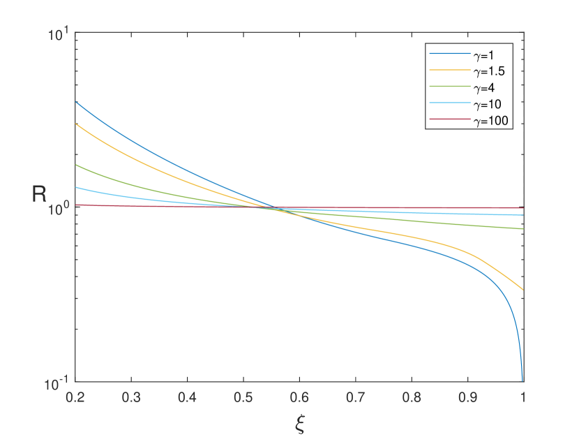
(a)

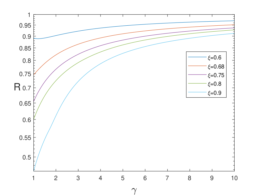
(b)

Figure 3: Upper bound on the risk of the batch-min-norm estimator with optimized batch size vs. (a) normalized $\mathsf{SNR}$ ($\xi$), and (b) overparametrization ratio $\gamma$. At moderate-to-high $\mathsf{SNR}$, the bound monotonically increases with $\gamma$.

Interestingly, things behave differently when the $\mathsf{SNR}$ is below $1$ ($\xi<1/2$). In this region, the bound on the risk of the optimized batch-min-norm has a single maxima point at some finite $\gamma$ value. This can be explained by the fact that at low enough $\mathsf{SNR}$, even after the batch partition which has a noise-smoothing / stabilizing effect, the $\mathsf{SNR}$ is still too low and the algorithm can do worst than the null risk in high overparameterization rates, just like the standard min-norm. Therefore, the risk reaches some maximal value at a finite $\gamma$, and then decreases to the null risk as $\gamma$ grows. This is essentially the double-descent phenomenon [14] which will be further discussed in Section 7.

Note that our optimal batch size analysis is taken with respect to the upper bound on the asymptotic risk, i.e., $n\rightarrow\infty$. In practice, one uses a finite number of data samples, in which case we need $b\ll n$ in order for $\mathrm{UB}(b,\gamma,\xi)$ to be reliable. Hence, there will be a finite (possibly very large) batch size $b$ that will minimize the risk for any pair $(\gamma,\xi)$.

6 Proof of Main Result

6.1 Asymptotic Bias

In order to estimate the asymptotic bias, we rewrite the $\operatorname{\mathsf{Bias}}(\hat{\boldsymbol{\beta}}_{\mathrm{BMN}})$ term from (20) as a recursive equation where at the $j$th step we add the $j$th batch $\boldsymbol{Y}_{j}$, that corresponds to the matrix rows $\boldsymbol{X}_{j}$, and update the contribution of this batch to the overall projection. Recall that

$$\boldsymbol{Y}_{j}=\boldsymbol{X}_{j}\boldsymbol{\beta}+\boldsymbol{W}_{j}=\boldsymbol{X}_{j}(\boldsymbol{\beta}+\boldsymbol{Z}_{j}),$$ (32)

with $\boldsymbol{Z}_{j}\triangleq\boldsymbol{X}_{j}^{T}(\boldsymbol{X}_{j}\boldsymbol{X}_{j}^{T})^{-1}\boldsymbol{W}_{j}$. Then, the $j$th row in the modified feature matrix $\boldsymbol{X}^{\prime}$ is

$$\boldsymbol{x}^{\prime}_{j}=\hat{\boldsymbol{\beta}}_{j}^{T}=(\boldsymbol{\beta}^{T}+\boldsymbol{Z}_{j}^{T})\boldsymbol{D}_{j},$$ (33)

with $\boldsymbol{D}_{j}$ the projection matrix onto the row space of $\boldsymbol{X}_{j}$. Denote by

$$\boldsymbol{X}^{\prime}_{j}=[\boldsymbol{x}^{\prime T}_{1},\cdots,\boldsymbol{x}^{\prime T}_{j}]^{T},$$ (34)

the modified feature matrix after the first $j$ steps and let $\boldsymbol{L}^{\prime}_{j}$ be the projection onto the row space of $\boldsymbol{X}^{\prime}_{j}$, that is

$$\boldsymbol{L}^{\prime}_{j}=\boldsymbol{X}^{\prime T}_{j}(\boldsymbol{X}^{\prime}_{j}\boldsymbol{X}^{\prime T}_{j})^{-1}\boldsymbol{X}^{\prime}_{j}.$$ (35)

Then, applying the rank-one update rule of the inverse of matrix product (see e.g. [39]) on $(\boldsymbol{X}^{\prime}_{j}\boldsymbol{X}^{\prime T}_{j})^{-1}$ we get

$$\|\boldsymbol{L}^{\prime}_{j}\boldsymbol{\beta}\|^{2}=\|\boldsymbol{L}^{\prime}_{j-1}\boldsymbol{\beta}\|^{2}+\mathbb{E}\left[\frac{((\boldsymbol{\beta}^{T}+\boldsymbol{Z}_{j}^{T})\boldsymbol{D}_{j}^{T}\left(\boldsymbol{I}-\boldsymbol{L}^{\prime}_{j-1}\right)\boldsymbol{\beta})^{2}}{(\boldsymbol{\beta}^{T}+\boldsymbol{Z}_{j}^{T})\boldsymbol{D}_{j}(\boldsymbol{I}-\boldsymbol{L}^{\prime}_{j-1})\boldsymbol{D}_{j}(\boldsymbol{\beta}+\boldsymbol{Z}_{j})}\right].$$ (36)

It can be seen that at each step the numerator of the update term in (36) is the projection of the part of $\boldsymbol{\beta}$ that lies in the null space of $\boldsymbol{L}^{\prime}_{j-1}$, namely the part of $\boldsymbol{\beta}$ that was not captured by the first $j-1$ rows of $\boldsymbol{X}^{\prime}$, onto the row space of the new batch. However, the projection is affected by the noise $\boldsymbol{Z}_{j}$ of the current batch. We can view this as a noisy version of the projection $\boldsymbol{D}_{j}$, a perspective that will be made clear in the next lemma, which is the key tool for analyzing the recursive rule (36).

Lemma 1.

Let $\boldsymbol{P}$ be a projection onto a subspace of dimension $\delta p$ for $\delta\in[0,1]$. Write $\|\boldsymbol{\beta}\|=r$ and $\|\boldsymbol{P}\boldsymbol{\beta}\|^{2}=\alpha r^{2}$ for $\alpha\in[0,1]$. Let $\{\boldsymbol{U}_{i}\}_{i=1}^{b}$ be uniformly drawn orthonormal vectors, and $\tilde{\boldsymbol{D}}$ a noisy projection onto the span of $\{\boldsymbol{U}_{i}\}$ given by

$$\tilde{\boldsymbol{D}}\boldsymbol{v}=\boldsymbol{D}\boldsymbol{v}+\sum_{i=1}^{b}\boldsymbol{U}_{i}Z_{i},$$ (37)

where $\boldsymbol{D}=\sum_{i=1}^{b}\boldsymbol{U}_{i}\boldsymbol{U}_{i}^{T}$, $Z_{i}\sim\mathcal{N}(0,T_{i}\cdot\sigma^{2}/p)$, and $T_{i}$ are r.vs. mutually independent of $\{\boldsymbol{U}_{i}\}$ and concentrated in the interval $[1-o(1),1+o(1)]$ with probability at least $1-o(1/p)$. Then, the expected squared noisy projection of $\boldsymbol{\beta}$ in the direction of $\boldsymbol{P}\tilde{\boldsymbol{D}}\boldsymbol{\beta}$ is given by

$$\mathbb{E}\left[\frac{\langle\boldsymbol{P}\tilde{\boldsymbol{D}}\boldsymbol{\beta},\boldsymbol{\beta}\rangle^{2}}{\|\boldsymbol{P}\tilde{\boldsymbol{D}}\boldsymbol{\beta}\|^{2}}\right]=\frac{1}{p}\left(\frac{\alpha r^{2}}{\delta}\left(1+(b-1)\cdot\frac{\alpha r^{2}}{\sigma^{2}+r^{2}}\right)+o(1)\right).$$ (38)

The remainder of this section is dedicated to the proof of Lemma 1, via a Gaussian approximation technique. But first, we use this lemma to prove the upper bound on the bias in Theorem 3.

Proof of bias part in Theorem 3..

Write

$$B_{j}=1-\frac{1}{r^{2}}\|\boldsymbol{L}^{\prime}_{j}\boldsymbol{\beta}\|^{2}$$ (39)

for the bias after $j$ steps. Since all of our results are normalized by $r$, we assume from now on that $r=1$. Then $B_{0}=1$, and the desired bias is given by

$$\lim_{p\rightarrow\infty}\operatorname{\mathsf{Bias}}\left(\hat{\boldsymbol{\beta}}_{\mathrm{BMN}}\right)=\lim_{p\rightarrow\infty}\mathbb{E}B_{\frac{n}{b}}.$$ (40)

Let $\boldsymbol{U}_{i},\cdots,\boldsymbol{U}_{b}$, be the orthonormal vectors that span the row space of $\boldsymbol{X}_{j}$, hence

$$\boldsymbol{D}_{j}=\sum_{i=1}^{b}\boldsymbol{U}_{i}\boldsymbol{U}_{i}^{T}.$$ (41)

Since the entries of $\boldsymbol{X}_{j}$ are i.i.d. $\mathcal{N}(0,1)$, then $\{\boldsymbol{U}_{i}\}$ are uniformly distributed. Moreover, $\boldsymbol{D}_{j}(\boldsymbol{\beta}+\boldsymbol{Z}_{j})$ can be written as a noisy projection as defined in the Lemma 1 (see Proposition 2 below). Denote $\bar{\boldsymbol{L}}_{j-1}\triangleq\boldsymbol{I}-\boldsymbol{L}^{\prime}_{j-1}$, then using Lemma 1 with $\boldsymbol{P}=\bar{\boldsymbol{L}}_{j-1}$ we get

$$\mathbb{E}\left[\frac{((\boldsymbol{\beta}^{T}+\boldsymbol{Z}_{j}^{T})\boldsymbol{D}_{j}^{T}\bar{\boldsymbol{L}}_{j-1}\boldsymbol{\beta})^{2}}{\|\bar{\boldsymbol{L}}_{j-1}\boldsymbol{D}_{j}(\boldsymbol{\beta}+\boldsymbol{Z}_{j})\|^{2}}\right] =\mathbb{E}\left[\frac{(\boldsymbol{\beta}^{T}\tilde{\boldsymbol{D}}_{j}^{T}\bar{\boldsymbol{L}}_{j-1}\boldsymbol{\beta})^{2}}{\boldsymbol{\beta}^{T}\tilde{\boldsymbol{D}}_{j}\bar{\boldsymbol{L}}_{j-1}\tilde{\boldsymbol{D}}_{j}\boldsymbol{\beta}}\right]$$ (42)

$$=\mathbb{E}\left[\frac{B_{j}(1+(b-1)\xi B_{j})}{\frac{p-j}{p}\cdot p}\right]+o(1/p),$$ (43)

where we set $\alpha=B_{j}$ and used the fact that with probability $1$ the dimension of $\bar{\boldsymbol{L}}_{j-1}$ is $\delta=1-j/p$. Then, from (36) we obtain

$$\mathbb{E}(B_{j+1}\mid B_{j})=B_{j}-\frac{B_{j}(1+(b-1)\xi B_{j})}{\frac{p-j}{p}\cdot p}+o(1/p),$$ (44)

and hence

$$\mathbb{E}B_{j+1}=\mathbb{E}B_{j}-\frac{\mathbb{E}B_{j}+(b-1)\xi\mathbb{E}B_{j}^{2}}{p-j}+o(1/p).$$ (45)

Define $t_{j}\triangleq\mathbb{E}B_{j}$. Then, using the (trivial) bound $\left(\mathbb{E}B_{j}\right)^{2}\leq\mathbb{E}B_{j}^{2}\leq\mathbb{E}B_{j}$ that holds for any random variable with support in the unit interval, we obtain

$$t_{j}\cdot\left(1-\frac{1+(b-1)\xi}{p-j}\right)+o(1/p)\leq t_{j+1}\leq t_{j}\cdot\left(1-\frac{1+(b-1)\xi t_{j}}{p-j}\right)+o(1/p).$$ (46)

We are interested in $t_{n/b}$ under the initial condition $t_{0}=1$, as $p\to\infty$ and $p/n=\gamma$ is held fixed. Noticing that over $n/b$ iterations of the recursive bound (46) the error term $o(1/p)$ can grow to at most $o(1)$, we drop it hereafter and add it back later. Note that for any $j\leq n/b$

$$\frac{d}{dt}t\left(1-\frac{1+(b-1)\xi t}{p-j}\right)=1-\frac{1+2(b-1)\xi t}{p-j}\geq 1-\frac{1}{p}\cdot\frac{1+2(b-1)\xi r^{2}}{(1-1/\gamma b)}.$$ (47)

Since the r.h.s of the above is positive for any large enough $p$, we get that the upper bound in (46) is monotonically increasing in $t_{j}$, and therefore we can use it iteratively. Specifically, any sequence of numbers $s_{0},\cdots,s_{n/b}$ with $s_{0}=1$ that obeys the right-hand-side inequality in (46) (replacing $t_{j}\to s_{j}$), will dominate the sequence $t_{0},\cdots,t_{n/b}$ in the sense that $t_{j}\leq s_{j}$, $j=0,\cdots,n/b$. To find such a sequence, let us rewrite the upper bound (46) as

$$\frac{t_{j+1}-t_{j}}{1/p}\leq\frac{t_{j}+(b-1)\xi t_{j}^{2}}{1-j/p}.$$ (48)

Now, suppose there exists a nonnegative convex function $g$ over $[0,1]$ with $g(0)=1$, satisfying

$$g^{\prime}(x)\leq\frac{g(x+1/p)-g(x)}{1/p}\leq-\frac{g(x)\cdot(1+(b-1)\xi g(x))}{1-x},$$ (49)

where the first inequality is by convexity of $g(x)$ and the second translates (48) to a differential inequality, replacing $t_{j}$ with $g(x)$ and $j/p$ with $x$. If we can find such a function, then taking $s_{j}=g(j/p)$ would yield the desired sequence. Let us show this is possible. First, rewrite (49) as

$$\frac{g^{\prime}(x)}{g(x)(1+(b-1)\xi g(x))}=\frac{d}{dx}\ln\left(\frac{g(x)}{1+(b-1)\xi g(x)}\right)\leq-\frac{1}{1-x}.$$ (50)

The initial condition is $\ln(g(0)/(1+(b-1)\xi g(0)))=-\ln(1+(b-1)\xi)$. Integrating we get

$$\ln\frac{g(x)}{1+(b-1)\xi g(x)} \leq-\ln(1+(b-1)\xi)-\int_{0}^{x}\frac{1}{1-x}dx=\ln\frac{1-x}{1+(b-1)\xi},$$ (51)

yielding $g(x)\leq\frac{1-x}{1+(b-1)\xi\cdot x}$, which is indeed nonnegative and convex over $[0,1]$. Hence, we have

$$t_{j}\leq g(j/p)\leq\frac{1-j/p}{1+(b-1)\xi\cdot j/p}.$$ (52)

Then, taking the limit with $j=n/b$ and adding back the error term, we get

$$\lim_{p\to\infty}\frac{1}{r^{2}}\operatorname{\mathsf{Bias}}\left(\hat{\boldsymbol{\beta}}_{\mathrm{BMN}}\right)\leq\lim_{p\to\infty}g(1/(\gamma b))+o(1)\leq\frac{\gamma b-1}{\gamma b+(b-1)\xi}.$$ (53)

∎

Next, we turn to prove Lemma 1. Let $\boldsymbol{S}=\left[\SS_{1},\cdots,\SS_{2b}\right]$ be a random vector given by

$$\SS_{i}\triangleq{\begin{cases}\langle\boldsymbol{P}\boldsymbol{U}_{i},\boldsymbol{\beta}\rangle,&i=1,\cdots b,\\ \langle(\boldsymbol{I}-\boldsymbol{P})\boldsymbol{U}_{i},\boldsymbol{\beta}\rangle,&i=b+1,\cdots,2b\end{cases}},$$ (54)

and define the function

$$f(\boldsymbol{s},\boldsymbol{z})\triangleq\frac{(\sum_{i=1}^{b}s_{i}\left(s_{i}+s_{b+i}+z_{i}\right))^{2}}{\sum_{i=1}^{b}\left(s_{i}+s_{b+i}+z_{i}\right)^{2}}.$$ (55)

The outline of the proof for Lemma 1 is as follows. First, in Lemma 2 we show that the expected squared projection (38) is approximately equal to $\mathbb{E}f(\boldsymbol{S},\boldsymbol{Z})$, for any noise $\boldsymbol{Z}$ that is sufficiently close in distribution to i.i.d. $\mathcal{N}(0,1/p)$ noise. Then, we show that $\mathbb{E}f(\boldsymbol{S},\boldsymbol{Z})$ can be calculated with good accuracy by replacing the vector $\boldsymbol{S}$ with a Gaussian vector $\boldsymbol{G}$ with independent entries that have the same variance as the elements of $\boldsymbol{S}$. To do so, in Lemma 3 we bound the Wasserstein distance between $\boldsymbol{S}$ and $\boldsymbol{G}$ using Corollary 1, and show that $f$ is Lipschitz where $\boldsymbol{S}$ and $\boldsymbol{G}$ are concentrated, hence $|\mathbb{E}f(\boldsymbol{S},\boldsymbol{Z})-\mathbb{E}f(\boldsymbol{G},\boldsymbol{Z})|\lessapprox\mathcal{W}_{1}(\boldsymbol{S},\boldsymbol{G})$. Then in Lemma 4 we explicitly calculate $\mathbb{E}f(\boldsymbol{G},\boldsymbol{Z})$ as a (random) weighted sum of MMSE estimators, yielding  (38) and concluding the proof.

First, we show that indeed $\mathbb{E}f(\boldsymbol{S},\boldsymbol{Z})$ approximates the mean-squared projection (38).

Lemma 2.

Let $\boldsymbol{S}$ be given by (54), $\boldsymbol{Z}=[Z_{1},\cdots,Z_{b}]$ as in Lemma 1, and $f(\boldsymbol{S},\boldsymbol{Z})$ as in (55). Then

$$\left|\mathbb{E}\left[\frac{1}{\delta}f(\boldsymbol{S},\boldsymbol{Z})\right]-\mathbb{E}\left[\frac{\langle\boldsymbol{P}\tilde{\boldsymbol{D}}\boldsymbol{\beta},\boldsymbol{\beta}\rangle^{2}}{\|\boldsymbol{P}\tilde{\boldsymbol{D}}\boldsymbol{\beta}\|^{2}}\right]\right|\leq\frac{1}{\sqrt[4]{p}}\cdot\mathbb{E}\left[\frac{1}{\delta}f(\boldsymbol{S},\boldsymbol{Z})\right]+o(1/p).$$ (56)

Proof.

See Appendix A.3. ∎

The above lemma shows that the update step we wish to evaluate in (36) is approximately given by $\mathbb{E}f(\boldsymbol{S},\boldsymbol{Z})$. Unfortunately, calculating $\mathbb{E}f(\boldsymbol{S},\boldsymbol{Z})$ w.r.t. the exact statistics of $\boldsymbol{S}$ is very challenging. Nevertheless, as the next corollary, which is a direct result of Theorem 2, shows that for large $p$ the vector $\boldsymbol{S}$ is close to Gaussian in the Wasserstein distance. This fact can then be utilized to approximate $\mathbb{E}f(\boldsymbol{S},\boldsymbol{Z})$.

Corollary 1.

Let $\boldsymbol{S}\in\mathbb{R}^{2b}$ be the random vector given in (54), and let $\boldsymbol{G}\in\mathbb{R}^{2b}$ have independent entries distributed as

$${G_{i}\sim\begin{cases}\mathcal{N}(0,\frac{\alpha}{p}),&i=1,\cdots b,\\ \mathcal{N}(0,\frac{1-\alpha}{p}),&i=b+1,\cdots,2b\end{cases}.}$$ (57)

Then $\mathcal{W}_{1}(\boldsymbol{S},\boldsymbol{G})\leq\sqrt{\frac{b}{p}}\cdot\frac{2\sqrt{2}b}{p-1}$.

Proof.

See Appendix A.3. ∎

We see that $\boldsymbol{S}$ in (54) is $O(p^{-3/2})$-close in Wasserstein distance to $\boldsymbol{G}$ in (57). If $f$ were $k$-Lipschitz in $\boldsymbol{s}$, this would yield a $O(kp^{-3/2})$ approximation for $\mathbb{E}f(\boldsymbol{S},\boldsymbol{Z})$, by calculating the latter using the Gaussian statistics. This is however not the case, since $f$’s gradient diverges along certain curves. Moreover, $f$ is also a function of the noise $\boldsymbol{Z}$. Nonetheless, we will show that $f$ is Lipschitz in the region where $\boldsymbol{S}$ and $\boldsymbol{G}$ are concentrated, which along with the fact that $\boldsymbol{Z}$ is independent of $\boldsymbol{S}$ and $\boldsymbol{G}$, will yield an upper bound on $|\mathbb{E}f(\boldsymbol{S},\boldsymbol{Z})-\mathbb{E}f(\boldsymbol{G},\boldsymbol{Z})|$.

Lemma 3.

Let $f:\mathbb{R}^{2b}\times\mathbb{R}^{b}\rightarrow\mathbb{R}$ be defined in (55), $\boldsymbol{S}$ and $\boldsymbol{Z}$ defined in (54) and Lemma 1, respectively, and $\boldsymbol{G}$ be distributed as in (57) and independent of $\boldsymbol{Z}$. Then,

$$\left|\mathbb{E}f(\boldsymbol{S},\boldsymbol{Z})-\mathbb{E}f(\boldsymbol{G},\boldsymbol{Z})\right|=o\left(1/p\right).$$ (58)

Proof.

See Appendix A.3 ∎

Lemma 4.

Let $\boldsymbol{G}$ be as in Lemma 1 and $\boldsymbol{Z}$ as in Lemma 1, then

$$\mathbb{E}\left[f(\boldsymbol{G},\boldsymbol{Z})\right]=\frac{\alpha r^{2}}{p}\left(1+(b-1)\xi\alpha\right)+o(1/p).$$ (59)

Proof.

See Appendix A.3 ∎

We are now ready to prove the main lemma of this section.

Proof of Lemma 1..

From Lemma 2 and Lemma 3 we get that

$$\left|\mathbb{E}\left[\frac{\langle\boldsymbol{P}\boldsymbol{D}\boldsymbol{\beta},\boldsymbol{\beta}\rangle^{2}}{\|\boldsymbol{P}\boldsymbol{D}\boldsymbol{\beta}\|^{2}}\right]-\mathbb{E}\left[\frac{1}{\delta}f(\boldsymbol{G},\boldsymbol{Z})\right]\right|\leq\frac{2}{\delta\sqrt[4]{p}}\cdot\mathbb{E}\left[f(\boldsymbol{G},\boldsymbol{Z})\right]+o\left(1/p\right).$$ (60)

Plugging in the result of Lemma 4 then yields

$$\Big{|}\mathbb{E}\left[\frac{\langle\boldsymbol{P}\boldsymbol{D}\boldsymbol{\beta},\boldsymbol{\beta}\rangle^{2}}{\|\boldsymbol{P}\boldsymbol{D}\boldsymbol{\beta}\|^{2}}\right] -\frac{\alpha(1+(b-1)\xi\alpha)}{\delta p}\Big{|}\leq$$ (61)

$$\frac{2}{\delta\sqrt[4]{p}}\cdot\left(\frac{\alpha(1+(b-1)\xi\alpha)}{\delta p}\right)+o\left(1/p\right)=o\left(1/p\right),$$ (62)

which concludes the proof. ∎

6.2 Asymptotic Variance

We now turn to evaluate the (asymptotic) variance term of batch-min-norm in (20). To do so, we note that by construction, the modified elements $Y^{\prime}_{j}$, $\boldsymbol{x}^{\prime}_{j}$ and $W^{\prime}_{j}$ are linear combinations of $\boldsymbol{Y}_{j}$, $\boldsymbol{X}_{j}$ and $\boldsymbol{W}_{j}$, respectively, with the exact same coefficients. Moreover, these coefficients converge almost surely to the batch samples $\boldsymbol{Y}_{j}$ as $p\to\infty$. We then use this observation to show that the variance $\operatorname{\mathsf{Var}}(\hat{\boldsymbol{\beta}}_{\mathrm{BMN}})$ converges almost surely to the variance of a Gaussian mixture vector multiplied by a large Wishart matrix, for which we derive an explicit asymptotic expression.

Recall that the $j$th modified sample is

$$Y^{\prime}_{j}=\boldsymbol{Y}_{j}^{T}(\boldsymbol{X}_{j}\boldsymbol{X}_{j}^{T})^{-1}\boldsymbol{X}_{j}\boldsymbol{\beta}+\boldsymbol{Y}_{j}^{T}(\boldsymbol{X}_{j}\boldsymbol{X}_{j}^{T})^{-1}\boldsymbol{W}_{j}=\boldsymbol{x}^{\prime T}_{j}\boldsymbol{\beta}+W^{\prime}_{j}$$ (63)

where $\boldsymbol{x}^{\prime}_{j}$ is a linear combination of the $j$th batch rows, with the coefficients

$$\boldsymbol{A}_{j}=\boldsymbol{Y}_{j}^{T}(\boldsymbol{X}_{j}\boldsymbol{X}_{j}^{T})^{-1}.$$ (64)

We proceed to analyze each batch separately. Denote the matrix rows in the $j$th batch by $\{\boldsymbol{x}_{ij}\}_{i=1}^{b}$, the noise elements by $\{W_{ij}\}_{i=1}^{b}$, and the samples by $\{Y_{ij}\}_{i=1}^{b}$. The modified feature vector resulting from the batch is

$$\boldsymbol{x}^{\prime}_{j}=\sum_{i=1}^{b}A_{ij}\boldsymbol{x}_{ij}.$$ (65)

Note that $\boldsymbol{x}^{\prime}_{j}$ are the weak min-norm per batch estimators, constituting the rows of the matrix $\boldsymbol{X}^{\prime}$. The modified sample is then

$$Y^{\prime}_{j}=\sum_{i=1}^{b}A_{ij}Y_{ij}=\sum_{i=1}^{b}A_{ij}\cdot(\langle\boldsymbol{x}_{ij},\boldsymbol{\beta}\rangle+W_{ij}),$$ (66)

and the associated modified noise is

$$W^{\prime}_{j}=\sum_{i=1}^{b}A_{ij}W_{ij}.$$ (67)

In what follows, we assume w.l.o.g. that $\boldsymbol{\beta}=[r,0\cdots,0]$, as our algorithm is invariant to rotations of $\boldsymbol{\beta}$. The key observation now is that the inverse Wishart matrix $(\frac{1}{p}\boldsymbol{X}_{j}\boldsymbol{X}_{j}^{T})^{-1}$ converges almost surely to identity, due to the strong law of large numbers. Denoting $\alpha_{ij}$ as the first entry of the vector $\boldsymbol{x}_{ij}$, this asymptotically yields

$$pA_{ij}=Y_{ij}=r\cdot\alpha_{ij}+W_{ij},$$ (68)

i.e., independent coefficients. In this case, given $\boldsymbol{Y}$, the modified feature matrix $\boldsymbol{X}^{\prime}$ has i.i.d. $\mathcal{N}(0,1)$ entries (except its first column), and the noise is independent and Gaussian. Using these ”clean” statistics, we can evaluate the variance term in (20), see Lemma 10. However, this is only asymptotically true, thus we need to show that the true variance term in (20) converges to the variance taken w.r.t. the ”clean” statistics. This is done next, in Lemma 5.

Lemma 5.

For the $j$th batch, define

$$Q_{j} =\sum_{i=1}^{b}Y_{ij}W_{ij}$$ (69)

$$\boldsymbol{f}_{j} =\sum_{i=1}^{b}Y_{ij}\boldsymbol{x}_{ij}.$$ (70)

Let $\boldsymbol{F}$ be the $n/b\times p$ matrix with $\{\boldsymbol{f}_{j}\}$ as its rows, and $\boldsymbol{Q}=[Q_{1},\cdots,Q_{n/b}]^{T}$. Then

$${\lim_{p\rightarrow\infty}\mathbb{E}\left[\boldsymbol{W}^{\prime T}(\boldsymbol{X}^{\prime}\boldsymbol{X}^{\prime T})^{-1}\boldsymbol{W}^{\prime}-\boldsymbol{Q}^{T}(\boldsymbol{F}\boldsymbol{F}^{T})^{-1}\boldsymbol{Q}\right]=0.}$$ (71)

In the above, note that $\boldsymbol{f}_{j}$ are random vectors constituting the rows of the random matrix $\boldsymbol{F}$.

Proof.

See Appendix A.4. ∎

Lemma 6.

Let $\boldsymbol{Q}$ and $\boldsymbol{F}$ be as in Lemma 5. Then

$${\lim_{p\rightarrow\infty}\mathbb{E}\left[\boldsymbol{Q}^{T}(\boldsymbol{F}\boldsymbol{F}^{T})^{-1}\boldsymbol{Q}\right]\leq\sigma^{2}\cdot\frac{b-(b-1)\xi}{(\gamma b-1)}.}$$ (72)

Proof.

See Appendix A.4. ∎

The proof of the variance bound in Theorem 3 follows directly from Lemmas 5 and 6, and thus conclude the proof for our main result in Theorem 3.

7 Numerical Results

Next, we demonstrate different aspects of the batch-min-norm estimator via numerical experiments. The setup for the simulations matches the linear model of Section 3. That is, isotropic feature matrix $\boldsymbol{X}$ with i.i.d. Standard Gaussian entries, and i.i.d. Gaussian noise vector $\boldsymbol{W}$, independent of $\boldsymbol{X}$, with zero mean and variance $\sigma^{2}$ that varies between the different experiments. The parameter vector $\boldsymbol{\beta}$ is normalized to have $\|\boldsymbol{\beta}\|=1$ unless explicitly mentioned otherwise.

The first experiment compares the performance of the batch-min-norm estimator to the asymptotic upper bound (21). Figure 4 depicts the risk vs. the overparameterization ratio $\gamma$, for two batch sizes (a) $b=2$ and (b) $b=4$, and four different $\mathsf{SNR}$ levels $\xi$, that correspond to $\sigma^{2}=2,1,\frac{1}{5},\frac{1}{20}$. The interpolation point in each of the batch size scenarios corresponds to $\gamma=1/b$. It can be seen that the upper bound (21) is tighter for smaller batch sizes. This is likely due to the fact that while the bound was derived in the limit $n,p\rightarrow\infty$ and for a fixed finite $b$, in practice we use a finite number of samples and parameters. Hence, as the batch size grows, the assumption $b\ll n,p$ that is used throughout the derivation of the bound, weakens.

In the two low $\mathsf{SNR}$ scenarios, we witness the double-descent phenomenon: the variance of the algorithm decreases as $\gamma$ grows. This was previously explained by [14] as the result of the additional degrees of freedom allowing for a solution $\boldsymbol{\beta}$ with a smaller $\ell_{2}$-norm to the linear model (16). As the $\ell_{2}$-norm of the estimator decreases, it converges to the null solution. In the two high $\mathsf{SNR}$ cases, a local minima of the risk is observed beyond the interpolation limit. This second bias-variance tradoff is due the fact that in the high $\mathsf{SNR}$ regime, when far enough from the interpolation point, the dominant factor in the risk is the bias, which grows with $\gamma$.

Batch-Min-Norm Risk and Upper Bound

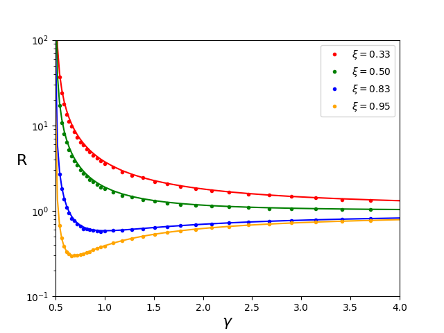
(a)

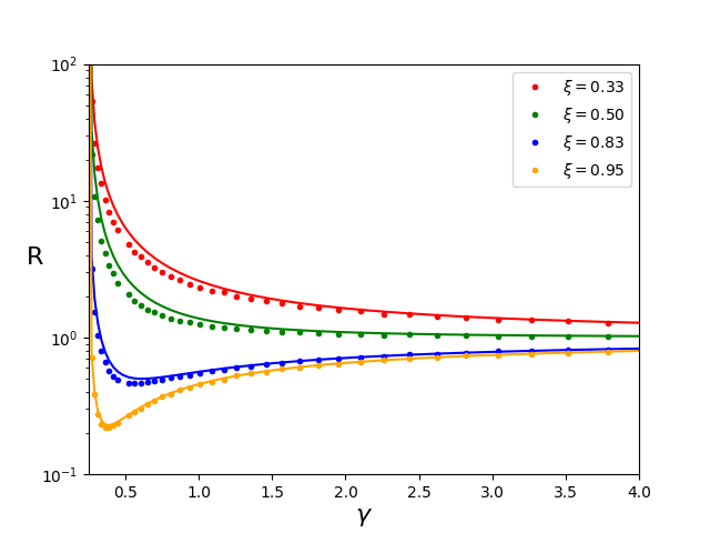
(b)

Figure 4: Batch-min-norm performance vs. overparameterizedrization ratio $\gamma$, for different values of $\xi$, with $p=500$ and batch sizes (a) $b=2$ and (b) $b=4$. The upper bounds appear as continuous lines and the algorithm performance is depicted using dot markers. In the low $\mathsf{SNR}$ cases $\xi=0.33$ and $\xi=0.5$ we witness the double-descent phenomenon, where the risk monotonically decreases with $\gamma$ beyond the interpolation point. In the high $\mathsf{SNR}$ curves $\xi=0.83$ and $\xi=0.95$ the risk has a local minima across the interpolation limit.

Next, we explore the effect of the batch size on the risk. Figure 5 presents the risk of different estimators vs. the overparameterization ratio $\gamma$. Three batch-min-norm estimators are presented, corresponding to batch sizes $b=1$ (which is equivalent in our case to regular min-norm estimation), $b=2$ and $b=20$. The interpolation point for each of the batch-min-norm estimators depends on the batch size. The performance of ridge regression with optimal regularization parameter is also presented. For completeness, we plot the risk below the interpolation points $\gamma b=1$ as well, though the analysis in this paper focuses on $\gamma b>1$. Subfigures 5-(b) and 5-(c) focus on each of the $\mathsf{SNR}$ levels in the overparameterized regime. As expected, optimally tuned ridge regression, which in the linear model setting is the linear minimum MSE estimator, has uniformly lower risk. In the low $\mathsf{SNR}$ scenario $\xi=0.5$, the variance of the algorithm is dominant, and larger batch sizes are preferable. This is due to the noise-averaging effect of the batch partition. In contrast, when $\xi=0.95$ the minimal batch size is optimal. This is because when the $\mathsf{SNR}$ increases, the bias becomes more dominant in the risk. Although the modified features $\boldsymbol{X}^{\prime}$ of the batch algorithm are favorably aligned with the parameter vector, the increased overparameterization ratio of the new problem still results in a larger bias. Hence as the weight of the bias in the risk grows, the optimal batch size decreases. Above some $\mathsf{SNR}$ threshold (that depend on $\gamma$), the minimal batch size $b=1$ is always preferable.

Risk for Different Algorithms

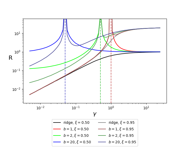
(a)

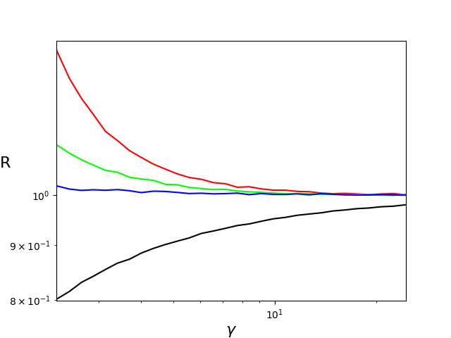
(b)

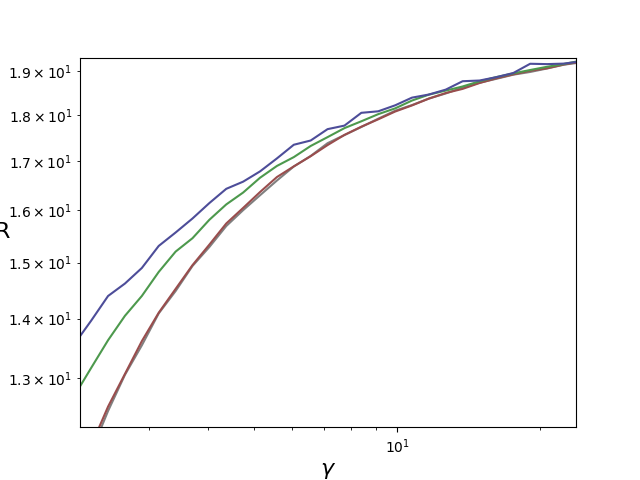
(c)

Figure 5: (a) Risk vs. overparameterization ratio $\gamma$ for two $\mathsf{SNR}$ levels $\xi$. The $\mathsf{SNR}$ levels were controlled by fixing $\sigma$ and varying $r$, hence the null risk $r^{2}$ is different between the two scenarios. Subfigures (b) and (c) zoom in on the high and low $\mathsf{SNR}$ clusters, respectively. It can be seen that while at high $\mathsf{SNR}$ large batch size achieves lower risk, when the $\mathsf{SNR}$ is low the minimal batch size $b=1$ is favorable.

The next experiment examines the risk of the batch-min-norm estimator vs. the batch size, with $\gamma=2$ and different $\mathsf{SNR}$ scenarios. Here the $\mathsf{SNR}$ level was controlled via fixing $\sigma^{2}$ and varying the signal energy $r^{2}$. Recall that in Section 5 the batch size was optimized with respect to the asymptotic upper bound. The results showed that as the $\mathsf{SNR}$ decreases or $\gamma$ reach the interpolation limit, the optimal batch size grows. Specifically, below the $\mathsf{SNR}$ threshold $\xi=0.6478$, increasing the batch size is always beneficial. However, as we demonstrated here in the first experiment (Fig. 4), the gap between the upper bound and actual risk grows with $b$. Therefore, as shown in Figure 6, in practice there is always some finite batch size that that achieves the minimal risk. For the lower $\mathsf{SNR}$ cases $\xi=0.5,0.6,0.7$, the optimal batch sizes are $18,15$ and $10$, respectively. When $\xi=0.8$ then $b=2$ achieves the minimal risk, and in the high $\mathsf{SNR}$ case $\xi=0.9$ the minimal batch size $b=1$ is optimal.

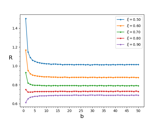
Figure 6: batch-min-norm risk vs. batch size for various values of $\xi$, with $p=2000$, $\gamma=2$. The $\mathsf{SNR}$ levels were controlled by fixing $\sigma$ and varying $r$, hence the null risk $r^{2}$ is different between the scenarios. It can be seen that for $\xi=0.5,0.6,0.7,0.8$, the optimal batch size is $b>1$, and for $\xi=0.9$ the phase transition discussed in Section 5 occurs, and the minimal risk is obtained at $b=1$ and monotonically increases thereafter.

Finally, we demonstrate the performance of the batch-min-norm estimator with optimized batch size. Figure 7 presents the risk of the optimized batch-min-norm vs. (a) normalized $\mathsf{SNR}$ $\xi$ with $\gamma=1.4$, and (b) overparameterization ratio $\gamma$ with $\xi=0.7$. Batch-min-norm is compared with four other algorithms: min-norm, batch-min-norm with $b=2$, ridge regression with optimal regularization parameter, and a naively stabilized version of min-norm, where samples are discarded to obtain the best possible risk (i.e., optimizing over all min-norm estimators with overparameterization ratio $\geq\gamma$). If $\gamma\leq\sqrt{\mathsf{SNR}}/(\sqrt{\mathsf{SNR}}-1)\triangleq\gamma_{\mathrm{opt}}$, optimized min-norm discards the required number of data samples in order to achieve overparametrization ratio $\gamma_{\mathrm{opt}}$, which in this case is the global minima for the min-norm estimator in the overparameterized regime ([14]). If $\gamma>\gamma_{\mathrm{opt}}$, all the samples are discarded and the null estimator is returned. As expected, the optimized batch-min-norm achieves lower risk than both min-norm and batch-min-norm with $b=2$, as they are both special cases of batch-min-norm. As the $\mathsf{SNR}$ grows, the optimal batch size decreases and the risk of the optimized batch-min-norm approaches that of min-norm. The two coincide for $\xi\geq 0.93$. The naively stabilized min-norm outperforms min-norm for any $\mathsf{SNR}$, as expected. It can be seen that for a wide range of $\mathsf{SNR}$ values, the optimized batch algorithm is better than the naive stabilization. When $\mathsf{SNR}=1$ (i.e., $\xi=0.5$), all algorithms except the ridge regression are no better than the null estimator. Hence in this range the optimized min-norm outperforms the optimized batch one, as it produces the null estimate. When the $\mathsf{SNR}$ is very high and $\gamma$ is close to the interpolation limit, the optimized min-norm also outperforms the optimized batch-min-norm, since in this case the optimal batch size is $b=1$, and $\gamma\leq\gamma_{\mathrm{opt}}$ .

Risk of Different Estimators

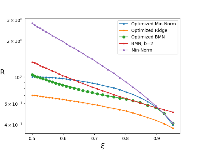
(a)

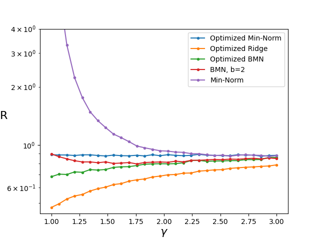
(b)

Figure 7: Risk of batch-min-norm with optimal batch size vs. (a) normalized $\mathsf{SNR}$ $\xi$, with $\gamma=1.4$, and (b) overparametrization ratio $\gamma$ with $\xi=0.7$.

Appendix A Additional Proofs and Results

A.1 The Wasserstein Distance

We state and prove some properties of the Wasserstein distance used in Section 6.1.

Proposition 1 (basic properties of Wasserstein distance).

The following properties hold for the $1$-Wasserstein distance

1. (triangle inequality) $\mathcal{W}_{1}(\mu,\nu)\leq\mathcal{W}_{1}(\mu,\gamma)+\mathcal{W}_{1}(\gamma,\nu)$.

2. (stability under linear transformations) Let $A$ be a deterministic matrix and $\boldsymbol{X},\boldsymbol{Y}$ two random vectors. Then

   $$\mathcal{W}_{1}(A\boldsymbol{X},A\boldsymbol{Y})\leq\|A\|_{F}\mathcal{W}_{1}(\boldsymbol{X},\boldsymbol{Y}).$$ (73)

3. If $\boldsymbol{X}$, $\boldsymbol{Y}\in\mathbb{R}^{n}$ and $\boldsymbol{Z}\in\mathbb{R}^{m}$ be mutually independent random vectors, then

   $$\mathcal{W}_{1}\left([\boldsymbol{X},\boldsymbol{Z}],[\boldsymbol{Y},\boldsymbol{Z}]\right)=\mathcal{W}_{1}(\boldsymbol{X},\boldsymbol{Y}).$$ (74)

Proof.

The proof of the first property is trivial and therefore omitted. For the second property, let $\gamma^{*}$ be the coupling that achieves the $1$-Wasserstein distance between the marginals of $\boldsymbol{X}$ and $\boldsymbol{Y}$, then

$$\|A\|_{F}\mathcal{W}_{1}(\boldsymbol{X},\boldsymbol{Y}) =\|A\|_{F}\mathbb{E}_{\gamma^{*}}\|\boldsymbol{X}-\boldsymbol{Y}\|^{p}\geq\mathbb{E}_{\gamma^{*}}\|A\boldsymbol{X}-A\boldsymbol{Y}\|_{2}\geq\mathcal{W}_{1}(A\boldsymbol{X},A\boldsymbol{Y}).$$ (75)

While proven here for $p=1$, the above property holds for any $p$ with the euclidean metric. Next, we prove the third property. Denote $\boldsymbol{X}\sim P_{\boldsymbol{X}}$, $\boldsymbol{Y}\sim P_{\boldsymbol{Y}}$ and $\boldsymbol{Z}\sim P_{\boldsymbol{Z}}$. Let $P_{\boldsymbol{X},\boldsymbol{Y}}$ be the coupling achieving the Wasserstein distance $\mathcal{W}_{1}(\boldsymbol{X},\boldsymbol{Y})$ between $\boldsymbol{X}$ and $\boldsymbol{Y}$, let $P_{\boldsymbol{Z},\boldsymbol{Z}^{\prime}}$ be a coupling of $\boldsymbol{Z}$ and $\boldsymbol{Z}^{\prime}$ that set $\Pr(\boldsymbol{Z}=\boldsymbol{Z}^{\prime})=1$, and let $\Gamma$ be the set of all couplings of $[\boldsymbol{X},\boldsymbol{Z}]$ and $[\boldsymbol{Y},\boldsymbol{Z}]$. Then, $P_{\boldsymbol{X},\boldsymbol{Y}}\otimes P_{\boldsymbol{Z},\boldsymbol{Z}^{\prime}}$ is a valid coupling for the marginals $P_{\boldsymbol{X}}\otimes P_{\boldsymbol{Z}}$ and $P_{\boldsymbol{Y}}\otimes P_{\boldsymbol{Z}}$ and therefore in $\Gamma$. Hence

$$\mathcal{W}_{1}\left([\boldsymbol{X},\boldsymbol{Z}],[\boldsymbol{Y},\boldsymbol{Z}]\right) \triangleq\inf_{\zeta\in\Gamma}\mathbb{E}_{\zeta}\sqrt{\|\boldsymbol{X}-\boldsymbol{Y}\|^{2}_{2}+\|\boldsymbol{Z}-\boldsymbol{Z}^{\prime}\|_{2}^{2}}$$ (76)

$$\leq\mathbb{E}_{P_{\boldsymbol{X},\boldsymbol{Y}}\otimes P_{\boldsymbol{Z},\boldsymbol{Z}^{\prime}}}\sqrt{\|\boldsymbol{X}-\boldsymbol{Y}\|^{2}_{2}+\|\boldsymbol{Z}-\boldsymbol{Z}^{\prime}\|_{2}^{2}}$$ (77)

$$=\mathbb{E}_{P_{\boldsymbol{X},\boldsymbol{Y}}}\sqrt{\|\boldsymbol{X}-\boldsymbol{Y}\|^{2}_{2}}$$ (78)

$$=\mathcal{W}_{1}(\boldsymbol{X},\boldsymbol{Y}).$$ (79)

In the above, we assumed that there exists a coupling $P_{\boldsymbol{X},\boldsymbol{Y}}$ that achieves $\mathcal{W}_{1}(\boldsymbol{X},\boldsymbol{Y})$. In the case that the infimum is obtained only in the limit, one can adjust the proof by taking the sequence of couplings that converge to the infimum. Since $\mathcal{W}_{1}\left([\boldsymbol{X},\boldsymbol{Z}],[\boldsymbol{Y},\boldsymbol{Z}]\right)$ is also trivially lower bounded by $\mathcal{W}_{1}\left(\boldsymbol{X},\boldsymbol{Y}\right)$, we get equality. ∎

The next lemma will demonstrate that when two measures are heavily concentrated on a bounded region, then conditioning on being in this region does not change the Wasserstein distance much.

Lemma 7 (stability).

Let $\boldsymbol{X}$ and $\boldsymbol{Y}$ be random vectors taking values in $\mathbb{R}^{n}$, and $\mathcal{D}\subset\mathbb{R}^{n}$ be a compact set such that $\Pr(\boldsymbol{X}\notin\mathcal{D})\leq\epsilon$ and $\Pr(\boldsymbol{Y}\notin\mathcal{D})\leq\delta$. Let $\boldsymbol{X}_{\mathcal{D}}$ and $\boldsymbol{Y}_{\mathcal{D}}$ denote the conditional random variables obtained from $\boldsymbol{X}$ and $\boldsymbol{Y}$ by conditioning on the events $\boldsymbol{X}\in\mathcal{D}$ and $\boldsymbol{Y}\in\mathcal{D}$, respectively. Then

$$\mathcal{W}_{1}(\boldsymbol{X}_{\mathcal{D}},\boldsymbol{Y}_{\mathcal{D}})\leq\mathcal{W}_{1}(\boldsymbol{X},\boldsymbol{Y})+(\epsilon+\delta)\cdot\max_{\boldsymbol{x},\boldsymbol{y}\in\mathcal{D}}\|\boldsymbol{x}-\boldsymbol{y}\|_{2}.$$ (80)

Proof.

Denote by $\mu$, $\nu$, $\tilde{\mu}$ and $\tilde{\nu}$ the pdf of $\boldsymbol{X}$, $\boldsymbol{Y}$, $\boldsymbol{X}_{\mathcal{D}}$ and $\boldsymbol{Y}_{\mathcal{D}}$, respectively. Let $(\boldsymbol{X}^{*},\boldsymbol{Y}^{*})\sim\zeta^{*}(\boldsymbol{x},\boldsymbol{y})$ be a coupling that attains the infimum in (1) (if there is no minimizer one can adjust the proof by taking a sequence of couplinngs that converges to the infimum). Define a new pair of random vectors $(\bar{\boldsymbol{X}},\bar{\boldsymbol{Y}})$ such that

$$(\bar{\boldsymbol{X}},\bar{\boldsymbol{Y}})=\begin{cases}(\boldsymbol{X}^{*},\boldsymbol{Y}^{*}),&(\boldsymbol{X}^{*},\boldsymbol{Y}^{*})\in\mathcal{D}^{2}\\ (\boldsymbol{A},\boldsymbol{Y}^{*}),&\boldsymbol{X}^{*}\notin\mathcal{D},\boldsymbol{Y}^{*}\in\mathcal{D},\\ (\boldsymbol{X}^{*},\boldsymbol{B}),&\boldsymbol{X}^{*}\in\mathcal{D},\boldsymbol{Y}^{*}\notin\mathcal{D},\\ (\boldsymbol{A},\boldsymbol{B}),&\boldsymbol{X}^{*}\notin\mathcal{D},\boldsymbol{Y}^{*}\notin\mathcal{D},\end{cases}$$ (81)

with $\boldsymbol{A}\sim\tilde{\mu}$, $\boldsymbol{B}\sim\tilde{\nu}$ being two random vectors such that $(\boldsymbol{X}^{*},\boldsymbol{Y}^{*}),\boldsymbol{A},\boldsymbol{B}$ are mutually independent. Denote by $a$ the probability that $(\boldsymbol{X}^{*},\boldsymbol{Y}^{*})\in\mathcal{D}^{2}$. Then on the one hand

$$\mathcal{W}_{1}(\boldsymbol{X},\boldsymbol{Y}) =\mathbb{E}\left[\|\boldsymbol{X}^{*}-\boldsymbol{Y}^{*}\|\right]$$ (82)

$$=a\cdot\mathbb{E}\left[\|\boldsymbol{X}^{*}-\boldsymbol{Y}^{*}\|\big{|}(\boldsymbol{X}^{*},\boldsymbol{Y}^{*})\in\mathcal{D}^{2}\right]+(1-a)\cdot\mathbb{E}\left[\|\boldsymbol{X}^{*}-\boldsymbol{Y}^{*}\|\big{|}(\boldsymbol{X}^{*},\boldsymbol{Y}^{*})\notin\mathcal{D}^{2}\right]$$ (83)

$$\geq a\cdot\mathbb{E}\left[\|\boldsymbol{X}^{*}-\boldsymbol{Y}^{*}\|\big{|}(\boldsymbol{X}^{*},\boldsymbol{Y}^{*})\in\mathcal{D}^{2}\right],$$ (84)

and on the other hand

$$\mathcal{W}_{1}(\boldsymbol{X}_{\mathcal{D}},\boldsymbol{Y}_{\mathcal{D}}) =\inf_{\zeta\in\Gamma[\tilde{\mu},\tilde{\nu}]}\mathbb{E}_{(\boldsymbol{X}^{\prime},\boldsymbol{Y}^{\prime})\sim\zeta}\|\boldsymbol{X}^{\prime}-\boldsymbol{Y}^{\prime}\|$$ (85)

$$\leq\mathbb{E}\|\bar{\boldsymbol{X}}-\bar{\boldsymbol{Y}}\|$$ (86)

$$=a\cdot\mathbb{E}\left[\|\bar{\boldsymbol{X}}-\bar{\boldsymbol{Y}}\|\big{|}(\boldsymbol{X}^{*},\boldsymbol{Y}^{*})\in\mathcal{D}^{2}\right]$$ (87)

$$\;\;\;+(1-a)\cdot\mathbb{E}\left[\|\bar{\boldsymbol{X}}-\bar{\boldsymbol{Y}}\|\big{|}(\boldsymbol{X}^{*},\boldsymbol{Y}^{*})\notin\mathcal{D}^{2}\right]$$ (88)

$$\leq a\cdot\mathbb{E}\left[\|\bar{\boldsymbol{X}}-\bar{\boldsymbol{Y}}\|\big{|}(\boldsymbol{X}^{*},\boldsymbol{Y}^{*})\in\mathcal{D}^{2}\right]+(1-a)\cdot R$$ (89)

$$=a\cdot\mathbb{E}\left[\|\boldsymbol{X}^{*}-\boldsymbol{Y}^{*}\|\big{|}(\boldsymbol{X}^{*},\boldsymbol{Y}^{*})\in\mathcal{D}^{2}\right]+(1-a)\cdot R.$$ (90)

$$\leq\mathcal{W}_{1}(\boldsymbol{X},\boldsymbol{Y})+(1-a)\cdot R,$$ (91)

where in (86) we used the fact that the coupling $(\bar{\boldsymbol{X}},\bar{\boldsymbol{Y}})$ has marginals $\tilde{\mu}$ and $\tilde{\nu}$, in (88) we used the total law of expectation, in (89) we used the fact that for any $\boldsymbol{x},\boldsymbol{y}\in\mathcal{D}$ we have $\|\boldsymbol{x}-\boldsymbol{y}\|_{2}\leq R$, and in (90) we used the fact that when $(\boldsymbol{X}^{*},\boldsymbol{Y}^{*})\in\mathcal{D}^{2}$ then $(\bar{\boldsymbol{X}},\bar{\boldsymbol{Y}})=(\boldsymbol{X}^{*},\boldsymbol{Y}^{*})$. Let us now bound $a$ from below

$$1-\delta\leq\Pr(\boldsymbol{Y}\in D)=\Pr(\boldsymbol{Y}^{*}\in D)=a+\Pr(\boldsymbol{Y}^{*}\in D,\boldsymbol{X}^{*}\not\in D)\leq a+\epsilon,$$ (92)

hence $a\geq 1-\epsilon-\delta$ and we get

$$\mathcal{W}_{1}(\boldsymbol{X}_{\mathcal{D}},\boldsymbol{Y}_{\mathcal{D}}) \leq\mathcal{W}_{1}(\boldsymbol{X},\boldsymbol{Y})+(\epsilon+\delta)\cdot R.$$ (93)

∎

A.2 Lower Bounds

Theorem 4.

The asymptotic risk of the batch min-norm algorithm is lower bounded by

$$\lim_{p\rightarrow\infty}R(\hat{\boldsymbol{\beta}}_{\mathrm{BMN}})\geq\left(1-\frac{1}{\gamma b}\right)^{1+(b-1)\xi}+\left|\frac{1-\xi}{\xi}\cdot\frac{1-\gamma b-(b-1)\xi}{\gamma b-1}\right|_{+}.$$ (94)

where the first (resp. second) addend lower bounds the asymptotic bias (resp. variance), and $|x|_{+}=\max(x,0)$.

It can be seen that the bounds on the bias in Theorem 3 and 4 are tight for either low $\mathsf{SNR}$ ($\xi\rightarrow 0$), high overparametrization ratio ($\gamma\rightarrow\infty$) or minimal batch size, $b=1$, in which case they coincide with the min-norm performance.

The variance upper bound also coincides with the one of the min-norm estimator for $b=1$. Moreover, it vanishes (for any $b$) as $\gamma$ grows, a phenomenon also known as double-descent ([14]). However, there is an additive $\frac{\sigma^{2}\gamma b}{\gamma b-1}$ gap between the upper and lower bounds on the variance. This gap is never negligible since $\gamma b>1$ and $0<\xi<1$. Note that in some cases the lower bound is trivial. Nonetheless, as we demonstrate later in the numerical experiments, the upper bound is quite tight in various scenarios.

To derive the lower bound we use the following lemma whose proof appears in Appendix A.4.

Lemma 8.

Let $\boldsymbol{Q}$ and $\boldsymbol{F}$ be as in Lemma 5. Then

$$\sigma^{2}\cdot\frac{b-\gamma b-(b-1)\xi}{\gamma b-1}\leq\lim_{p\rightarrow\infty}\mathbb{E}\left[\boldsymbol{Q}^{T}\left(\boldsymbol{F}\boldsymbol{F}^{T}\right)^{-1}\boldsymbol{Q}\right].$$ (95)

Proof of Theorem 4..

To derive the lower bound on the bias, recall (46) and note that the lower bound there yields

$$\ln t_{j} \geq\sum_{\ell=0}^{j-1}\ln\left(1-\frac{1+(b-1)\xi}{p-\ell}\right)$$ (96)

$$=-\sum_{\ell=0}^{j-1}\left(\frac{1+(b-1)\xi}{p-\ell}\right)$$ (97)

$$=-\sum_{\ell=0}^{j-1}\left(\frac{1}{p}\cdot\frac{1+(b-1)\xi}{1-\frac{\ell}{p}}\right)$$ (98)

$$\geq-(1+(b-1)\xi)\int_{0}^{j/p}\frac{dx}{1-x}$$ (99)

$$=(1+(b-1)\xi)\cdot\ln(1-j/p)$$ (100)

and so, after adding back the error term we get

$$t_{j}\geq(1-j/p)^{1+(b-1)\xi}\cdot e^{o(1)}.$$ (101)

Specifically, we see that the (normalized) asymptotic bias is lower bounded by

$$\lim_{p\to\infty}\operatorname{\mathsf{Bias}}\left(\hat{\boldsymbol{\beta}}_{\mathrm{BMN}}\right)=\lim_{p\to\infty}t_{n/b}\geq\left(1-\frac{1}{\gamma b}\right)^{1+(b-1)\xi}.$$ (102)

The lower bound on the variance follows immediately from Lemmas 5 and 8.

∎

A.3 Proof of the Lemmas in Subsection 6.1

To prove Lemma 2 we will use the following proposition.

Proposition 2.

Let $\boldsymbol{D}_{j}$ be the projection onto the row space of $\boldsymbol{X}_{j}$, and let $\boldsymbol{Z}_{j}\triangleq\boldsymbol{X}_{j}^{T}(\boldsymbol{X}_{j}\boldsymbol{X}_{j}^{T})^{-1}\boldsymbol{W}_{j}$, then $\boldsymbol{D}_{j}(\boldsymbol{\beta}+\boldsymbol{Z}_{j})$ can be written as a noisy projection of the form (37).

Proof.

Let $\boldsymbol{U}_{1},\cdots,\boldsymbol{U}_{b}$ be the orthonormal basis vectors for the subspace spans by the rows $\boldsymbol{X}_{j}$, then

$$\boldsymbol{D}_{j}(\boldsymbol{\beta}+\boldsymbol{Z}_{j})=\boldsymbol{D}_{j}\boldsymbol{\beta}+\boldsymbol{D}_{j}\boldsymbol{X}_{j}^{T}(\boldsymbol{X}_{j}\boldsymbol{X}_{j}^{T})^{-1}\boldsymbol{W}_{j}=\boldsymbol{D}_{j}\boldsymbol{\beta}+\sum_{i=1}^{b}\boldsymbol{U}_{i}\lambda_{i}W_{ij},$$ (103)

with $\lambda_{i}\triangleq\lambda_{i}((\boldsymbol{X}_{j}\boldsymbol{X}_{j})^{-1/2})$ and $W_{ij}$ the $i$th element of $\boldsymbol{W}_{j}$. Since $\boldsymbol{X}_{j}$ is i.i.d. Gaussian, it is well-known that the eigenvalues $\{\lambda_{i}\}$ are mutually independent of the eigenvectors $\{\boldsymbol{U}_{i}\}$. Define $T_{i}\triangleq p\lambda_{i}^{2}$ and $Z_{i}\triangleq\lambda_{i}W_{ij}$, then $Z_{i}\sim\mathcal{N}(0,T_{i}\cdot\frac{\sigma^{2}}{p})$. As required in the conditions of Lemma 1, $T_{i}$, $i=1,\cdots,b$, are highly concentrated around $1$, and specifically we have (see for example Corollary 5.35 in [40])

$$\Pr\left(\sqrt{\frac{T_{i}}{p}}\in\left[\frac{1}{\sqrt{p}}-\frac{1}{p^{-\frac{7}{8}}},\frac{1}{\sqrt{p}}+\frac{1}{p^{-\frac{7}{8}}}\right]\right)\geq 1-2e^{-\frac{\sqrt[4]{p}}{2}}.$$ (104)

∎

Proof of Lemma 2..

The proof for this lemma is based on the fact that for a large $p$, the length $\|\boldsymbol{P}\boldsymbol{U}_{i}\|^{2}\approx\delta$ and $\langle\boldsymbol{P}\boldsymbol{U}_{i},P\boldsymbol{U}_{j}\rangle\approx 0$. If this was true with equality, then by noticing that

$$\langle\boldsymbol{P}\tilde{\boldsymbol{D}}\boldsymbol{\beta},\boldsymbol{\beta}\rangle =\langle\sum_{i}\boldsymbol{P}\boldsymbol{U}_{i}\left(\boldsymbol{U}_{i}^{T}\boldsymbol{\beta}+Z_{i}\right),\boldsymbol{\beta}\rangle$$ (105)

$$=\sum_{i}\left(\langle\boldsymbol{U}_{i},\boldsymbol{\beta}\rangle+Z_{i}\right)\cdot\langle\boldsymbol{P}\boldsymbol{U}_{i},\boldsymbol{\beta}\rangle$$ (106)

$$=\sum_{i=1}^{b}\SS_{i}\cdot(\SS_{i}+\SS_{b+i}+Z_{i})$$ (107)

and

$$\|\boldsymbol{P}\tilde{\boldsymbol{D}}\boldsymbol{\beta}\|^{2} =\langle\boldsymbol{P}\tilde{\boldsymbol{D}}\boldsymbol{\beta},\boldsymbol{P}\tilde{\boldsymbol{D}}\boldsymbol{\beta}\rangle$$ (108)

$$=\langle\sum_{i}\boldsymbol{P}\boldsymbol{U}_{i}\left(\boldsymbol{U}_{i}^{T}\boldsymbol{\beta}+Z_{i}\right),\sum_{i}\boldsymbol{P}\boldsymbol{U}_{i}\left(\boldsymbol{U}_{i}^{T}\boldsymbol{\beta}+Z_{i}\right)\rangle$$ (109)

$$=\langle\sum_{i}(\langle\boldsymbol{U}_{i},\boldsymbol{\beta}\rangle+Z_{i})\cdot\boldsymbol{P}\boldsymbol{U}_{i}\,,\sum_{i}(\langle\boldsymbol{U}_{i},\boldsymbol{\beta}\rangle+Z_{i})\cdot\boldsymbol{P}\boldsymbol{U}_{i}\rangle$$ (110)

$$=\sum_{i}(\SS_{i}+\SS_{b+i}+Z_{i})^{2}\cdot\|\boldsymbol{P}\boldsymbol{U}_{i}\|^{2}$$ (111)

$$\quad+\sum_{i\neq\ell}(\langle\boldsymbol{U}_{i},\boldsymbol{\beta}\rangle+Z_{i})\cdot(\langle\boldsymbol{U}_{\ell},\boldsymbol{\beta}\rangle+Z_{\ell})\cdot\langle\boldsymbol{P}\boldsymbol{U}_{i},P\boldsymbol{U}_{\ell}\rangle,$$ (112)

we would have got $\frac{1}{\delta}f(\boldsymbol{S},\boldsymbol{Z})=\frac{\langle\boldsymbol{P}\tilde{\boldsymbol{D}}\boldsymbol{\beta},\boldsymbol{\beta}\rangle^{2}}{\|\boldsymbol{P}\tilde{D}\boldsymbol{\beta}\|^{2}}$.

To show that this is asymptotically true let us define $E_{i}\triangleq\|\boldsymbol{P}\boldsymbol{U}_{i}\|^{2}-\delta$, $i=1,\cdots,b$, and $C_{i\ell}\triangleq\langle\boldsymbol{P}\boldsymbol{U}_{i},P\boldsymbol{U}_{\ell}\rangle$, $i\neq j\in\{1,\cdots,b\}$. Then, define the events

$$\mathcal{E} =\left\{\{|\mathbb{E}_{i}|\leq\epsilon,i=1\cdots,b\}\;\cap\;\{|C_{i\ell}|\leq\ \epsilon,\;\forall i\neq\ell\}\right\},$$ (113)

$$\mathcal{Z} =\left\{|Z_{i}|<a,i=1,\cdots,b\right\}.$$ (114)

Denote by $\bar{\mathcal{E}}$ and $\bar{\mathcal{Z}}$ the complement events of $\mathcal{E}$ and $\mathcal{Z}$, respectively, and note that $\mathcal{E}$ and $\mathcal{Z}$ are independent. From the triangle inequality we get

$$\Bigg{|}\mathbb{E}\Big{[}\frac{1}{\delta}f(\boldsymbol{S},\boldsymbol{Z})\Big{]}-\mathbb{E}\Big{[} \frac{\langle\boldsymbol{P}\tilde{\boldsymbol{D}}\boldsymbol{\beta},\boldsymbol{\beta}\rangle^{2}}{\|\boldsymbol{P}\tilde{\boldsymbol{D}}\boldsymbol{\beta}\|^{2}}\Big{]}\Bigg{|}\leq\underset{T_{1}}{\underbrace{\left|\mathbb{E}\left[\frac{\langle\boldsymbol{P}\tilde{\boldsymbol{D}}\boldsymbol{\beta},\boldsymbol{\beta}\rangle^{2}}{\|\boldsymbol{P}\tilde{\boldsymbol{D}}\boldsymbol{\beta}\|^{2}}\right]-\mathbb{E}\left[\frac{\langle\boldsymbol{P}\tilde{\boldsymbol{D}}\boldsymbol{\beta},\boldsymbol{\beta}\rangle^{2}}{\|\boldsymbol{P}\tilde{\boldsymbol{D}}\boldsymbol{\beta}\|^{2}}\Big{|}\mathcal{E}\cap\mathcal{Z}\right]\right|}}$$ (115)

$$+\underset{T_{2}}{\underbrace{\left|\mathbb{E}\left[\frac{\langle\boldsymbol{P}\tilde{\boldsymbol{D}}\boldsymbol{\beta},\boldsymbol{\beta}\rangle^{2}}{\|\boldsymbol{P}\tilde{\boldsymbol{D}}\boldsymbol{\beta}\|^{2}}\Big{|}\mathcal{E}\cap\mathcal{Z}\right]-\mathbb{E}\left[\frac{1}{\delta}f(\boldsymbol{S},\boldsymbol{Z})\Big{|}\mathcal{E}\cap\mathcal{Z}\right]\right|}}$$ (116)

$$+\underset{T_{3}}{\underbrace{\left|\mathbb{E}\left[\frac{1}{\delta}f(\boldsymbol{S},\boldsymbol{Z})\Big{|}\mathcal{E}\cap\mathcal{Z}\right]-\mathbb{E}\left[\frac{1}{\delta}f(\boldsymbol{S},\boldsymbol{Z})\right]\right|}}.$$ (117)

We now estimate the above terms $T_{1},T_{2},T_{3}$.

First, let us look at $T_{1}$. Let $\epsilon=\frac{\delta}{2b\sqrt[4]{p}}$ , then using the total law of expectation we get

$$\mathbb{E}\left[\frac{\langle\boldsymbol{P}\tilde{\boldsymbol{D}}\boldsymbol{\beta},\boldsymbol{\beta}\rangle^{2}}{\|\boldsymbol{P}\tilde{\boldsymbol{D}}\boldsymbol{\beta}\|^{2}}\right]- \mathbb{E}\left[\frac{\langle\boldsymbol{P}\tilde{\boldsymbol{D}}\boldsymbol{\beta},\boldsymbol{\beta}\rangle^{2}}{\|\boldsymbol{P}\tilde{\boldsymbol{D}}\boldsymbol{\beta}\|^{2}}\Big{|}\mathcal{E}\cap\mathcal{Z}\right]\leq\Pr(\bar{\mathcal{E}}\cup\bar{\mathcal{Z}})\times$$ (118)

$$\left(\mathbb{E}\left[\frac{\langle\boldsymbol{P}\tilde{\boldsymbol{D}}\boldsymbol{\beta},\boldsymbol{\beta}\rangle^{2}}{\|\boldsymbol{P}\tilde{\boldsymbol{D}}\boldsymbol{\beta}\|^{2}}\Big{|}\bar{\mathcal{E}}\cup\bar{\mathcal{Z}}\right]-\mathbb{E}\left[\frac{\langle\boldsymbol{P}\tilde{\boldsymbol{D}}\boldsymbol{\beta},\boldsymbol{\beta}\rangle^{2}}{\|\boldsymbol{P}\tilde{\boldsymbol{D}}\boldsymbol{\beta}\|^{2}}\Big{|}\mathcal{E}\cap\mathcal{Z}\right]\right).$$ (119)

Using Cauchy-Schwarz and the union bound we get that for any event $\mathcal{A}$

$$\Pr(\bar{\mathcal{E}}\cup\bar{\mathcal{Z}})\mathbb{E}\left[\frac{\langle\boldsymbol{P}\tilde{\boldsymbol{D}}\boldsymbol{\beta},\boldsymbol{\beta}\rangle^{2}}{\|\boldsymbol{P}\tilde{\boldsymbol{D}}\boldsymbol{\beta}\|^{2}}\Big{|}\mathcal{A}\right] \leq\left(\Pr(\bar{\mathcal{E}})+\Pr(\bar{\mathcal{Z}})\right)\mathbb{E}\left[\frac{\|\boldsymbol{P}\tilde{\boldsymbol{D}}\boldsymbol{\beta}\|^{2}\|\boldsymbol{\beta}\|^{2}}{\|\boldsymbol{P}\tilde{\boldsymbol{D}}\boldsymbol{\beta}\|^{2}}\Big{|}\mathcal{A}\right]$$ (120)

$$=\left(\Pr(\bar{\mathcal{E}})+\Pr(\bar{\mathcal{Z}})\right)\cdot r^{2}.$$ (121)

From the Johnson–Lindenstrauss lemma (see for example Lemma 2.2 in [41]) we get that

$$\Pr\left(\left|\|\boldsymbol{P}\boldsymbol{U}_{i}\|^{2}-\delta\right|\geq\epsilon\right)\leq e^{-\frac{\epsilon^{2}p}{2\delta}},\;\;\Pr\left(|\langle\boldsymbol{P}\boldsymbol{U}_{i},\boldsymbol{P}\boldsymbol{U}_{j}\rangle|\geq\epsilon\right)\leq e^{-\frac{\epsilon^{2}p}{8}}.$$ (122)

Therefore, for our choice of $\epsilon$ we get

$$\Pr\left(\bar{\mathcal{E}}\right)\leq 2b^{2}e^{-\frac{\delta\sqrt{p}}{64b}}$$ (123)

Also from the concentration properties of $T_{i}$ we have that

$$\Pr(|Z_{i}|>a) =\mathbb{E}\Pr(|Z_{i}|>a|T_{i})$$ (124)

$$\leq 1\cdot\Pr\left(|Z_{i}|>a\big{|}T_{i}=1+o(1)\right)$$ (125)

$$\;\;\;+o(1/p)\cdot\Pr\left(|Z_{i}|>a\big{|}T_{i}=1+\omega(1)\right)$$ (126)

$$\leq e^{-\frac{a^{2}(p+o(p))}{2\sigma^{2}}}+o(1/p)=o(1/p),$$ (127)

where in (127) we used the bound $\Pr(\mathcal{N}(0,1)\geq x)\leq\exp\{-x^{2}/2\}$ and the concentration property of $T_{i}$. Therefore we get

$$\left|\mathbb{E}\left[\frac{\langle\boldsymbol{P}\tilde{\boldsymbol{D}}\boldsymbol{\beta},\boldsymbol{\beta}\rangle^{2}}{\|\boldsymbol{P}\tilde{\boldsymbol{D}}\boldsymbol{\beta}\|^{2}}\right]-\mathbb{E}\left[\frac{\langle\boldsymbol{P}\tilde{\boldsymbol{D}}\boldsymbol{\beta},\boldsymbol{\beta}\rangle^{2}}{\|\boldsymbol{P}\tilde{\boldsymbol{D}}\boldsymbol{\beta}\|^{2}}\Big{|}\mathcal{E}\cap\mathcal{Z}\right]\right|=o(1/p).$$ (128)

In a similar way, and using the fact that $0\leq f(\boldsymbol{S},\boldsymbol{Z})\leq br^{2}$, we get for $T_{3}$

$$\left|\mathbb{E}\left[\frac{1}{\delta}f(\boldsymbol{S},\boldsymbol{Z})\right]-\mathbb{E}\left[\frac{1}{\delta}f(\boldsymbol{S},\boldsymbol{Z})\Big{|}\mathcal{E}\cap\mathcal{Z}\right]\right|=o(1/p)$$ (129)

In order to bound $T_{2}$ note that from (105) and (108) we get

$$\frac{\langle\boldsymbol{P}\tilde{\boldsymbol{D}}\boldsymbol{\beta},\boldsymbol{\beta}\rangle^{2}}{\|\boldsymbol{P}\tilde{\boldsymbol{D}}\boldsymbol{\beta}\|^{2}}=\frac{1}{\delta}f(\boldsymbol{S},\boldsymbol{Z})\cdot\frac{1}{1+\frac{\sum_{i}E_{i}\left(\langle\boldsymbol{U}_{i},\boldsymbol{\beta}\rangle+Z_{i}\right)^{2}}{\delta\sum_{i}\left(\langle\boldsymbol{U}_{i},\boldsymbol{\beta}\rangle+Z_{i}\right)^{2}}+\frac{\sum_{i\neq j}C_{ij}\left(\langle\boldsymbol{U}_{i},\boldsymbol{\beta}\rangle+Z_{i}\right)\cdot\left(\langle\boldsymbol{U}_{j},\boldsymbol{\beta}\rangle+Z_{j}\right)}{\delta\sum_{i}\left(\langle\boldsymbol{U}_{i},\boldsymbol{\beta}\rangle+Z_{i}\right)^{2}}}.$$ (130)

Hence, using the Taylor expansion $\frac{1}{1+x}=\sum_{\ell=0}^{\infty}(-x)^{\ell}$ we get

$$\Big{|}\mathbb{E}\Big{[}\frac{\langle\boldsymbol{P}\tilde{\boldsymbol{D}}\boldsymbol{\beta},\boldsymbol{\beta}\rangle^{2}}{\|\boldsymbol{P}\tilde{\boldsymbol{D}}\boldsymbol{\beta}\|^{2}} \Big{|}\mathcal{E}\cap\mathcal{Z}\Big{]}-\mathbb{E}\left[\frac{1}{\delta}f(\boldsymbol{S},\boldsymbol{Z})\Big{|}\mathcal{E}\cap\mathcal{Z}\right]\Big{|}$$ (131)

$$\leq\Big{|}\mathbb{E}\Big{[}\frac{1}{\delta}f(\boldsymbol{S},\boldsymbol{Z})\Big{(}\frac{\sum_{i}|E_{i}|(\langle\boldsymbol{U}_{i},\boldsymbol{\beta}\rangle+Z_{i})^{2}}{\delta\sum_{i}(\langle\boldsymbol{U}_{i},\boldsymbol{\beta}\rangle+Z_{i})^{2}}$$ (132)

$$\qquad+\frac{\sum_{i\neq j}|C_{ij}|(\langle\boldsymbol{U}_{i},\boldsymbol{\beta}\rangle+Z_{i})\cdot(\langle\boldsymbol{U}_{j},\boldsymbol{\beta}\rangle+Z_{j})}{\delta\sum_{i}(\langle\boldsymbol{U}_{i},\boldsymbol{\beta}\rangle+Z_{i})^{2}}\Big{)}\Big{|}\mathcal{E}\cap\mathcal{Z}\Big{]}\Big{|}$$ (133)

$$\leq\frac{2b\epsilon}{\delta}\mathbb{E}\left[\frac{1}{\delta}f(\boldsymbol{S},\boldsymbol{Z})\Big{|}\mathcal{E}\cap\mathcal{Z}\right]$$ (134)

$$\leq\frac{1}{\sqrt[4]{p}}\left(\mathbb{E}\left[\frac{1}{\delta}f(\boldsymbol{S},\boldsymbol{Z})\right]+o(1/p)\right).$$ (135)

Combining (128), (131) and (129) we get

$$\left|\mathbb{E}\left[\frac{1}{\delta}f(\boldsymbol{S},\boldsymbol{Z})\right]-\mathbb{E}\left[\frac{\langle\boldsymbol{P}\tilde{\boldsymbol{D}}\boldsymbol{\beta},\boldsymbol{\beta}\rangle^{2}}{\|\boldsymbol{P}\tilde{\boldsymbol{D}}\boldsymbol{\beta}\|^{2}}\right]\right| \leq\frac{1}{\sqrt[4]{p}}\cdot\mathbb{E}\left[\frac{1}{\delta}f(\boldsymbol{S},\boldsymbol{Z})\right]+o(1/p)$$ (136)

∎

Proof of Corollary 1..

This corollary is a direct result of Theorem 2, since $\boldsymbol{S}$ is a low-rank projection of the uniformly random orthonormal matrix $\boldsymbol{U}\triangleq[\boldsymbol{U}_{1},\cdots,\boldsymbol{U}_{b}]$ onto a subspace of dimension $2b$. Let $\boldsymbol{A}_{i}$ be a $p\times p$ matrix with all zeros except for the $i$th row which is given by $\sqrt{\frac{p}{\alpha}}\boldsymbol{\beta}^{T}\boldsymbol{P}$ and $\boldsymbol{B}_{i}$ be a $p\times p$ matrix with all zeros except for the $i$th row which is given by $\sqrt{\frac{p}{1-\alpha}}\boldsymbol{\beta}^{T}(\boldsymbol{I}-\boldsymbol{P})$. Note that $\SS_{i}=\sqrt{\frac{\alpha}{p}}\operatorname{Tr}{(\boldsymbol{A}_{i}\boldsymbol{U})}$, and $\SS_{b+i}=\sqrt{\frac{1-\alpha}{p}}\operatorname{Tr}{(\boldsymbol{B}_{i}\boldsymbol{U})}$, $i=1,\cdots,b$, and define the length $2b$ random vector $\tilde{\boldsymbol{S}}$ such that $\tilde{\SS}_{i}\triangleq\operatorname{Tr}{(\boldsymbol{A}_{i}\boldsymbol{U})}=\sqrt{\frac{p}{\alpha}}\cdot\SS_{i}$, and $\tilde{\SS}_{b+i}\triangleq\operatorname{Tr}{(\boldsymbol{A}_{i}\boldsymbol{U})}=\sqrt{\frac{p}{1-\alpha}}\cdot\SS_{b+i}$, $i=1,\cdots,b$. Then, since we have

$$\operatorname{Tr}{(\boldsymbol{A}_{i}\boldsymbol{A}_{j}^{T})}=p\cdot\mathds{1}\left(i=j\right),\;\;\operatorname{Tr}{(\boldsymbol{B}_{i}\boldsymbol{B}_{j}^{T})}=p\cdot\mathds{1}\left(i=j\right),\;\;\operatorname{Tr}{(\boldsymbol{A}_{i}\boldsymbol{B}_{j}^{T})}=0,\forall i,j.$$ (137)

we get from Theorem 2 that

$$\mathcal{W}_{1}(\tilde{\boldsymbol{S}},\tilde{\boldsymbol{G}})\leq\frac{2\sqrt{2}b}{p-1}.$$ (138)

where $\tilde{\boldsymbol{G}}$ is i.i.d. Gaussian with zero mean and unit variance. Let $\Lambda$ be a $b\times b$ diagonal matrix with first $b$ diagonal elements equal to $\sqrt{\frac{\alpha}{p}}$ and last $b$ elements equal to $\sqrt{\frac{1-\alpha}{p}}$. Then, by noting that $\boldsymbol{S}=\Lambda\tilde{\boldsymbol{S}}$, $\boldsymbol{G}=\Lambda\tilde{\boldsymbol{G}}$ we get that

$$\mathcal{W}_{1}(\boldsymbol{S},\boldsymbol{G})\leq\|\Lambda\|_{F}\mathcal{W}_{1}(\tilde{\boldsymbol{S}},\tilde{\boldsymbol{G}})=\sqrt{b\cdot\frac{\alpha}{p}+b\cdot\frac{1-\alpha}{p}}\mathcal{W}_{1}(\tilde{\boldsymbol{S}},\tilde{\boldsymbol{G}})\leq\sqrt{\frac{b}{p}}\cdot\frac{2\sqrt{2}b}{p-1}.$$ (139)

∎

The following Lemmas shows that indeed $f$ is Lipschitz over the region where $\boldsymbol{S}$ and $\boldsymbol{G}$ are concentrated on. This is needed for the proof of Lemma 3.

Lemma 9.

Let $\boldsymbol{G}$ be as in (57), $\boldsymbol{S}$ be as in (54) and $\boldsymbol{Z}$ be as in Lemma 1, and let $f$ be as in (55). Then there exists a constant $C$ that does not depend on $p$, and a set $\mathcal{D}$ with diameter no larger than $C$, over which $f$ is $C$-Lipschitz and concentrated:

$$\Pr\left((\boldsymbol{S},\boldsymbol{Z})\in\mathcal{D}\right)=1-o(1/p),\;\;\Pr\left((\boldsymbol{G},\boldsymbol{Z})\in\mathcal{D}\right)=1-o(1/p),$$ (140)

Proof.

We will show that the gradient of $f$ is bounded with sufficiently high probability under both distributions, and that the corresponding high probability set is bounded. To that end, let us write $v_{i}=s_{i}+s_{b+i}+z_{i}$. The partial derivatives of $f$ are given by

$$\frac{\partial f(\boldsymbol{s},\boldsymbol{z})}{\partial s_{\ell}} =2(s_{\ell}+v_{\ell})\cdot\frac{\langle\boldsymbol{s},\boldsymbol{v}\rangle}{\|\boldsymbol{v}\|^{2}}-2v_{\ell}\cdot\frac{|\langle\boldsymbol{s},\boldsymbol{v}\rangle|^{2}}{\|\boldsymbol{v}\|^{4}},$$ (141)

$$\frac{\partial f(\boldsymbol{s},\boldsymbol{z})}{\partial s_{b+\ell}} =\frac{\partial f(\boldsymbol{s},\boldsymbol{z})}{\partial z_{\ell}}=2s_{\ell}\cdot\frac{\langle\boldsymbol{s},\boldsymbol{v}\rangle}{\|\boldsymbol{v}\|^{2}}-2v_{\ell}\cdot\frac{|\langle\boldsymbol{s},\boldsymbol{v}\rangle|^{2}}{\|\boldsymbol{v}\|^{4}}.$$ (142)

For brevity, we perform the analysis using the more difficult random vector $\boldsymbol{S}$, and note that all our derivations hold verbatim for the Gaussian $\boldsymbol{G}$. Also, we will only analyze the term $v_{\ell}\cdot|\langle\boldsymbol{s},\boldsymbol{v}\rangle|^{2}/\|\boldsymbol{v}\|^{4}$ in the partial derivatives, as the other terms follow similarly (and are in fact statistically smaller, hence easier).

First, recalling that $\boldsymbol{Z}$ is a zero mean i.i.d.  Gaussian vector and variances $\sigma^{2}/p$, we have

$$\Pr(\|\boldsymbol{V}\|^{2}\leq\epsilon) \leq\Pr(\|\boldsymbol{V}\|_{\infty}\leq\sqrt{\epsilon})$$ (143)

$$=\mathbb{E}\prod_{i=1}^{b}\Pr(|V_{i}|\leq\sqrt{\epsilon}|S_{i})$$ (144)

$$=\mathbb{E}\prod_{i=1}^{b}\Pr(|Z_{i}+S_{i}|\leq\sqrt{\epsilon}|S_{i})$$ (145)

$$\leq\prod_{i=1}^{b}\Pr(|Z_{i}|\leq\sqrt{\epsilon})$$ (146)

$$\leq\left(\frac{\epsilon p}{\sigma^{2}}\right)^{b/2}$$ (147)

where we have used the standard anti-concentration inequality for the Gaussian distribution. Let us therefore pick $\epsilon=\Theta(p^{-(1+2/b)})$, under which this event has $o(1/p)$ probability. Furthermore, note that $\Pr(\|\boldsymbol{S}\|_{\infty}>\frac{\log^{2}p}{\sqrt{p}})=o(1/p)$ as well as $\Pr(\|\boldsymbol{Z}\|_{\infty}>\frac{\log^{2}p}{\sqrt{p}})=o(1/p)$, and hence $\Pr(\|\boldsymbol{V}\|_{\infty}>\frac{\log^{2}p}{\sqrt{p}})=o(1/p)$, which all remain order-wise the same when conditioned on the high-probability $1-o(1/p)$ event where $\|\boldsymbol{V}\|^{2}>\epsilon=\Theta(p^{-(1+2/b)})$. Thus, with probability $1-o(1/p)$ we have that

$$|V_{\ell}|\cdot\frac{|\langle\boldsymbol{S},\boldsymbol{V}\rangle|^{2}}{\|\boldsymbol{v}\|^{4}} \leq\|\boldsymbol{V}\|_{\infty}\cdot\frac{\|\boldsymbol{S}\|^{2}}{\|\boldsymbol{V}\|^{2}}=O(\frac{\log^{2}p}{\sqrt{p}})\cdot O(\frac{\log^{4}p}{p})\cdot\Theta(p^{1+2/b})$$ (148)

$$=O\left(p^{2/b-1/2}\cdot\log^{6}p\right),$$ (149)

which is bounded for $b>4$. It can be trivially verified that a similar analysis shows the boundedness of the first term in the partial derivatives, and a more subtle version of this analysis yields the same result for any $b\geq 1$. This immediately implies a bounded gradient (and hence Lipschitzness) over the set defined by the norm constraints above, and it is easy to see that this set is also bounded, concluding the proof.

∎

Proof of Lemma 3..

First, note that that $Z_{i}$ is independent of $\boldsymbol{U}_{i}$, $i=1,\cdots,b$, and therefore the vectors $\boldsymbol{S}$ and $\boldsymbol{Z}$ are independent. From Lemma 9 we get that there exist a set $\mathcal{D}$ on which $f$ is $C$-Lipschitz and both $t\triangleq\Pr((\boldsymbol{G},\boldsymbol{Z})\notin\mathcal{D})=o(1/p)$ and $t^{\prime}\triangleq\Pr((\boldsymbol{S},\boldsymbol{Z})\notin\mathcal{D})=o(1/p)$. Let $(\boldsymbol{G},\boldsymbol{Z})_{\mathcal{D}}$ (resp. $(\boldsymbol{S},\boldsymbol{Z})_{\mathcal{D}}$) be the random vector $(\boldsymbol{G},\boldsymbol{Z})$ (resp. $(\boldsymbol{S},\boldsymbol{Z})$) conditioned on the event $(\boldsymbol{G},\boldsymbol{Z})\in\mathcal{D}$ (resp. $(\boldsymbol{S},\boldsymbol{Z})\in\mathcal{D}$) and $(\boldsymbol{G},\boldsymbol{Z})_{\bar{\mathcal{D}}}$ (resp. $(\boldsymbol{S},\boldsymbol{Z})_{\bar{\mathcal{D}}}$) be $(\boldsymbol{G},\boldsymbol{Z})$ (resp. $(\boldsymbol{S},\boldsymbol{Z})$) conditioned on the complementary event $(\boldsymbol{G},\boldsymbol{Z})\notin\mathcal{D}$ (resp. $(\boldsymbol{S},\boldsymbol{Z})\notin\mathcal{D}$). Then,

$$\Big{|}\mathbb{E}f(\boldsymbol{S},\boldsymbol{Z})-\mathbb{E}f(\boldsymbol{G},\boldsymbol{Z})\Big{|}= \Big{|}\mathbb{E}f((\boldsymbol{S},\boldsymbol{Z})_{\mathcal{D}})-\mathbb{E}f((\boldsymbol{G},\boldsymbol{Z})_{\mathcal{D}})$$ (150)

$$+t^{\prime}\left(\mathbb{E}f((\boldsymbol{S},\boldsymbol{Z})_{\bar{\mathcal{D}}})-\mathbb{E}f((\boldsymbol{S},\boldsymbol{Z})_{\mathcal{D}})\right)$$ (151)

$$+t\left(\mathbb{E}f((\boldsymbol{G},\boldsymbol{Z})_{\mathcal{D}})-\mathbb{E}f((\boldsymbol{G},\boldsymbol{Z})_{\bar{\mathcal{D}}})\right)\Big{|}.$$ (152)

Recall that

$$f(\boldsymbol{S},\boldsymbol{Z})\leq\sum_{i=1}^{b}\SS_{i}^{2}\leq br,$$ (154)

hence

$$\left|t^{\prime}\left(\mathbb{E}f((\boldsymbol{S},\boldsymbol{Z})_{\bar{\mathcal{D}}})-\mathbb{E}f((\boldsymbol{S},\boldsymbol{Z})_{\mathcal{D}})\right)\right|\leq 2br^{2}o(1/p).$$ (155)

From Lemma 9 we get that $f(\boldsymbol{s},\boldsymbol{z})$ is Lipschitz over $\mathcal{D}\times\mathbb{R}^{b}$ with some Lipschitz constant $C(a,b)$ that does not depend on $p$. Since $\mathcal{D}$ has bounded diameter $C$ and $f$ is $C$-Lipschitz on $\mathcal{D}$ we get

$$\Big{|}\mathbb{E}f(\boldsymbol{S}, \boldsymbol{Z})_{\mathcal{D}}-\mathbb{E}f(\boldsymbol{G},\boldsymbol{Z})_{\mathcal{D}}\Big{|}\leq C\cdot\mathcal{W}\left((\boldsymbol{S},\boldsymbol{Z})_{\mathcal{D}},(\boldsymbol{G},\boldsymbol{Z})_{\mathcal{D}}\right)$$ (156)

$$\leq C\left(\mathcal{W}_{1}((\boldsymbol{S},\boldsymbol{Z}),(\boldsymbol{G},\boldsymbol{Z}))+(t+t^{\prime})\cdot\max_{(\boldsymbol{s},\boldsymbol{z}),(\boldsymbol{g},\boldsymbol{z}^{\prime})\in\mathcal{D}}\|(\boldsymbol{s},\boldsymbol{z})-(\boldsymbol{g},\boldsymbol{z}^{\prime})\|\right)$$ (157)

$$\leq C\left(\mathcal{W}_{1}(\boldsymbol{S},\boldsymbol{G})+(t+t^{\prime})\cdot\max_{(\boldsymbol{s},\boldsymbol{z}),(\boldsymbol{g},\boldsymbol{z}^{\prime})\in\mathcal{D}}\|(\boldsymbol{s},\boldsymbol{z})-(\boldsymbol{g},\boldsymbol{z}^{\prime})\|\right)$$ (158)

$$\leq C\cdot\sqrt{\frac{b}{p}}\cdot\frac{2\sqrt{2}b}{p-1}+C\cdot o(1/p)$$ (159)

where in (156) we used the dual representation (2) of the Wasserstein distance from Theorem 1, in (157) we used Lemma 7 along with the fact that $\mathcal{D}$ has bounded diameter, in (158) we used Proposition 1 along with the fact that $\boldsymbol{Z}$ is independent of $\boldsymbol{S}$ and $\boldsymbol{G}$, and in (159) we used (139). Finally, note that since $\boldsymbol{G}$ is independent Gaussian and the diameter $C$ of $\mathcal{D}$ does not depend on $p$, we have $t=e^{-\omega(p)}$, we get

$$t\mathbb{E}f((\boldsymbol{G},\boldsymbol{Z})_{\bar{\mathcal{D}}})\leq t\cdot\sum_{i=1}^{b}\mathbb{E}G_{\bar{\mathcal{D}},i}^{2}=b\cdot 2\int_{a}^{\infty}y^{2}e^{-\frac{py^{2}}{2\alpha}}dy\leq\frac{2b\alpha}{p}\cdot(a+1)\cdot e^{-\frac{pa^{2}}{\alpha}}.$$ (160)

and also

$$t\mathbb{E}f((\boldsymbol{G},\boldsymbol{Z})_{{\mathcal{D}}})\leq t^{\prime}bC^{2}=o(1/p).$$ (161)

where we used the relation

$$\int_{a}^{\infty}y^{2}e^{-\frac{py^{2}}{\alpha}}dy=-y\cdot\frac{\alpha}{p}e^{-\frac{py^{2}}{2\alpha}}\Big{|}_{a}^{\infty}+\int_{a}^{\infty}\frac{\alpha}{p}e^{-\frac{py^{2}}{2\alpha}}dy\leq a\cdot\frac{\alpha}{p}e^{-\frac{pa^{2}}{2\alpha}}+\frac{\alpha^{2}}{p^{2}}e^{-\frac{pa^{2}}{2\alpha}}$$ (162)

Plugging (155), (159), (160) and (161) back to (150) we get

$$\left|\mathbb{E}f(\boldsymbol{S},\boldsymbol{Z})-\mathbb{E}f(\boldsymbol{G},\boldsymbol{Z})\right| =o(1/p)$$ (163)

∎

Proof of Lemma 4..

Recall that $f(\boldsymbol{G},\boldsymbol{Z})=\frac{\left(\sum_{i=1}^{b}G_{i}\left(G_{i}+G_{b+i}+Z_{i}\right)\right)^{2}}{\sum_{i=1}^{b}\left(G_{i}+G_{b+i}+Z_{i}\right)^{2}}$ , where $Z_{i}\sim\mathcal{N}(0,T_{i}\sigma^{2}/p)$, and $T_{i}$ are concentrated on the interval $[t_{\mathrm{min}},t_{\mathrm{max}}]$ with probability $1-o(1/p)$, where

$$t_{\mathrm{min}}=1-o(1),\;\;t_{\mathrm{max}}=1+o(1).$$ (164)

Denote $\boldsymbol{T}=[T_{1},\cdots,T_{b}]$, let $\mathcal{U}$ be the event that $\boldsymbol{T}\in[t_{\mathrm{min}},t_{\mathrm{max}}]^{b}$, and let $\bar{\mathcal{U}}$ be its complement. Then,

$$\mathbb{E}f(\boldsymbol{G},\boldsymbol{Z})=\mathbb{E}\left[f(\boldsymbol{G},\boldsymbol{Z})\Big{|}\mathcal{U}\right]+\Pr(\bar{\mathcal{U}})\left(\mathbb{E}\left[f(\boldsymbol{G},\boldsymbol{Z})\Big{|}\bar{\mathcal{U}}\right]-\mathbb{E}\left[f(\boldsymbol{G},\boldsymbol{Z})\Big{|}\mathcal{U}\right]\right).$$ (165)

Using the bound $f(\boldsymbol{G},\boldsymbol{Z})\leq\sum_{i=1}^{b}G_{i}^{2}$ and the fact that $\{G_{i}\}$ are independent of $\boldsymbol{T}$ and therefore of $\mathcal{U}$, we get

$$\left|\Pr(\bar{\mathcal{U}})\left(\mathbb{E}\left[f(\boldsymbol{G},\boldsymbol{Z})\Big{|}\bar{\mathcal{U}}\right]-\mathbb{E}\left[f(\boldsymbol{G},\boldsymbol{Z})\Big{|}\mathcal{U}\right]\right)\right| \leq 2\Pr(\bar{\mathcal{U}})\mathbb{E}\left[\sum_{i=1}^{b}G_{i}^{2}\right]$$ (166)

$$\leq 4\frac{\alpha}{p}\cdot o(1/p),$$ (167)

which implies that

$$\left|\mathbb{E}f(\boldsymbol{G},\boldsymbol{Z})-\mathbb{E}\left[f(\boldsymbol{G},\boldsymbol{Z})\Big{|}\mathcal{U}\right]\right|=o(1/p^{2}).$$ (168)

To estimate $\mathbb{E}[f(\boldsymbol{G},\boldsymbol{Z})|\mathcal{U}]$, note that $f(\boldsymbol{G},\boldsymbol{Z})$ depends on $\boldsymbol{Z}_{i}$ only through the sum $G_{i}+G_{b+i}+Z_{i}\triangleq A_{i}$, hence we can write $f(\boldsymbol{G},\boldsymbol{Z})=\bar{f}(\boldsymbol{G},\boldsymbol{A})$, for $\boldsymbol{A}=[A_{1},\cdots,A_{b}]$. Further note that given $\boldsymbol{T}=[t_{1},\cdots,t_{b}]\triangleq\boldsymbol{t}$, the variables $A_{i}$, $i=1,\cdots,b$, are mutually independent and Gaussian. Denote by $\bar{G}_{i}$ the random variable obtain from $G_{i}$ by conditioning on the events $\mathcal{U}$, $\boldsymbol{A}=\boldsymbol{a}$ and $\boldsymbol{T}=\boldsymbol{t}$, then

$$\bar{G}_{i} \sim\mathcal{N}\left(\frac{\alpha r^{2}/p}{r^{2}/p+\sigma^{2}t_{i}/p}\cdot a_{i},\frac{\frac{\alpha r^{2}}{p}\left(\frac{(1-\alpha)r^{2}}{p}+\sigma^{2}t_{i}/p\right)}{\frac{r^{2}}{p}+\sigma^{2}t_{i}/p}\right)$$ (169)

$$=\mathcal{N}\left(\xi_{i}\alpha a_{i},\,\frac{\alpha\xi_{i}}{p}\cdot\left((1-\alpha)r^{2}+\sigma^{2}t_{i}\right)\right),$$ (170)

where $\xi_{i}=r^{2}/(r^{2}+\sigma^{2}t_{i})$. Denote $\eta_{i}\triangleq\frac{\alpha\xi_{i}}{p}\cdot\left((1-\alpha)r^{2}+\sigma^{2}t_{i}\right)$, then

$$\mathbb{E}\left[f(\boldsymbol{G},\boldsymbol{Z})\mid\mathcal{U}\right] =\mathbb{E}\left[\mathbb{E}\left[\bar{f}(\bar{\boldsymbol{G}},\boldsymbol{a})\right]\Big{|}\mathcal{U}\right],$$ (171)

and

$$\mathbb{E}\left[\frac{1}{\|\boldsymbol{a}\|^{2}}\left(\sum_{i=1}^{b}a_{i}\bar{G}_{i}\right)^{2}\right]=\frac{1}{\|\boldsymbol{a}\|^{2}}\left(\left(\sum a_{i}^{2}\xi_{i}\right)^{2}\alpha^{2}+\sum a_{i}^{2}\eta_{i}\right),$$ (172)

where we used the fact that $\sum_{i=1}^{b}a_{i}\bar{G}_{i}\sim\mathcal{N}(\sum a_{i}^{2}\xi_{i}\alpha,\sum a_{i}^{2}\eta_{i})$. Next, note that $\xi_{i}\in[\xi_{\mathrm{min}},\xi_{\mathrm{max}}]$ and $\eta_{i}\in[\eta_{\mathrm{min}},\eta_{\mathrm{max}}]$, for all $i=1,\cdots,b$, where

$$\xi_{\mathrm{min}} \triangleq\frac{r^{2}}{r^{2}+t_{\mathrm{max}}\sigma^{2}},$$ (173)

$$\xi_{\mathrm{max}} \triangleq\frac{r^{2}}{r^{2}+t_{\mathrm{min}}\sigma^{2}},$$ (174)

$$\eta_{\mathrm{min}} \triangleq\frac{\alpha\xi_{\mathrm{min}}}{p}\cdot\left((1-\alpha)r^{2}+\sigma^{2}t_{\mathrm{min}}\right),$$ (175)

$$\eta_{\mathrm{max}} \triangleq\frac{\alpha\xi_{\mathrm{max}}}{p}\cdot\left((1-\alpha)r^{2}+\sigma^{2}t_{\mathrm{max}}\right).$$ (176)

Using the above to bound (172) we get

$$\|\boldsymbol{a}\|^{2}\xi_{\mathrm{min}}^{2}\alpha^{2}+\eta_{\mathrm{min}}\leq\mathbb{E}\bar{f}(\bar{\boldsymbol{G}},\boldsymbol{a})\leq\|\boldsymbol{a}\|^{2}\xi_{\mathrm{max}}^{2}\alpha^{2}+\eta_{\mathrm{max}},$$ (177)

Since given $\boldsymbol{T}=\boldsymbol{t}$ the variables $A_{i}\sim\mathcal{N}(0,(r^{2}+t_{i}\sigma^{2})/p)$ are mutually independent, we get

$$\mathbb{E}\Big{[}\bar{f}(\boldsymbol{G},\boldsymbol{A} )\mid\boldsymbol{T}=\boldsymbol{t},\mathcal{U}\Big{]}\leq\xi_{\mathrm{max}}^{2}\alpha^{2}\sum_{i=1}^{b}\mathbb{E}\left[A_{i}^{2}\Big{|}\boldsymbol{T}=\boldsymbol{t},\mathcal{U}\right]+\eta_{\mathrm{max}}$$ (178)

$$=\left(\xi_{\mathrm{max}}^{2}\alpha^{2}\cdot\sum_{i=1}^{b}\left(r^{2}/p+\sigma^{2}t_{i}/p\right)+\frac{\alpha\xi_{\mathrm{max}}}{p}\cdot\left((1-\alpha)r^{2}+\sigma^{2}t_{\mathrm{max}}\right)\right)$$ (179)

$$\leq\left(\xi_{\mathrm{max}}^{2}\alpha^{2}\cdot b\left(r^{2}/p+\sigma^{2}t_{\mathrm{max}}/p\right)+\frac{\alpha\xi_{\mathrm{max}}}{p}\cdot\left((1-\alpha)r^{2}+\sigma^{2}t_{\mathrm{max}}\right)\right)$$ (180)

$$=\left(\frac{r^{2}\alpha^{2}b}{p}\cdot\frac{r^{2}+\sigma^{2}t_{\mathrm{max}}}{\left(r^{2}+\sigma^{2}t_{\mathrm{min}}\right)^{2}}+\frac{\alpha\xi_{\mathrm{max}}}{p}\cdot\left((1-\alpha)r^{2}+\sigma^{2}t_{\mathrm{max}}\right)\right)$$ (181)

$$=\frac{\alpha r^{2}}{p}\left(1+(b-1)\xi\alpha\right)+o(1/p),$$ (182)

where $\xi$ is the normalized $\mathsf{SNR}$, and we used the fact that $t_{\mathrm{max}}=1+o(1)$, and

$$\xi_{\mathrm{max}} =\frac{r^{2}}{r^{2}+\sigma^{2}-\sigma^{2}\cdot o(1)}=\xi\cdot\frac{1}{1-\frac{\sigma^{2}}{r^{2}+\sigma^{2}}\cdot o(1)}=\xi+o(1),$$ (183)

$$\frac{r^{2}+\sigma^{2}t_{\mathrm{max}}}{\left(r^{2}+\sigma^{2}t_{\mathrm{min}}\right)^{2}} =\frac{r^{2}+\sigma^{2}}{(r^{2}+\sigma^{2}(1-o(1))}+\frac{\sigma^{2}\cdot o(1)}{(r^{2}+\sigma^{2}(1-o(1))}=\frac{1}{r^{2}+\sigma^{2}}+o(1).$$ (184)

In a similar way we get the lower bound

$$\mathbb{E}\left[\bar{f}(\boldsymbol{G},\boldsymbol{A})\mid\boldsymbol{T}=\boldsymbol{t},\mathcal{U}\right] \geq\frac{\alpha r^{2}}{p}\left(1+(b-1)\xi\alpha\right)+o(1/p).$$ (185)

Since the bounds we got does not depend on $\boldsymbol{t}$, we get

$$\mathbb{E}\left[f(\boldsymbol{G},\boldsymbol{Z})\mid\mathcal{U}\right] =\mathbb{E}\left[\bar{f}(\boldsymbol{G},\boldsymbol{A})\mid\mathcal{U}\right]=\frac{\alpha r^{2}}{p}\left(1+(b-1)\xi\alpha\right)+o(1/p),$$ (186)

and combining with (168) we get the result of lemma. ∎

Proof of Lemma 1..

From Lemma 3 and Lemma 2 we get that

$$\left|\mathbb{E}\left[\frac{\langle\boldsymbol{P}\boldsymbol{D}\boldsymbol{\beta},\boldsymbol{\beta}\rangle^{2}}{\|\boldsymbol{P}\boldsymbol{D}\boldsymbol{\beta}\|^{2}}\right]-\mathbb{E}\left[\frac{1}{\delta}f(\boldsymbol{G},\boldsymbol{Z})\right]\right|\leq\frac{2}{\delta\sqrt[4]{p}}\cdot\mathbb{E}\left[f(\boldsymbol{G},\boldsymbol{Z})\right]+o\left(1/p\right).$$ (187)

Plugging in the result of Lemma 4 yields

$$\left|\mathbb{E}\left[\frac{\langle\boldsymbol{P}\boldsymbol{D}\boldsymbol{\beta},\boldsymbol{\beta}\rangle^{2}}{\|\boldsymbol{P}\boldsymbol{D}\boldsymbol{\beta}\|^{2}}\right]-\frac{\alpha(1+(b-1)\xi\alpha)}{\delta p}\right| \leq\frac{2}{\delta\sqrt[4]{p}}\cdot\left(\frac{\alpha(1+(b-1)\xi\alpha)}{\delta p}\right)+o\left(1/p\right)$$ (188)

$$=o\left(1/p\right).$$ (189)

∎

A.4 Proof of the Lemmas in Subsection 6.2

We will make use in the following two propositions.

Proposition 3.

Let $\boldsymbol{F}$ be a $n\times p$ matrix, $n<p$, such that

$$\boldsymbol{F}=\left[\boldsymbol{t}\;\;\boldsymbol{F}^{\prime}\right],$$ (190)

that is, $\boldsymbol{t}$ is the first column of $\boldsymbol{F}$ and $\boldsymbol{F}^{\prime}$ is a matrix composed of the remaining columns. Then, for any vector $\boldsymbol{x}$,

$$\boldsymbol{x}^{T}\left(\boldsymbol{F}\boldsymbol{F}^{T}\right)^{-1}\boldsymbol{x}\leq\boldsymbol{x}^{T}\left(\boldsymbol{F}^{\prime}\boldsymbol{F}^{\prime T}\right)^{-1}\boldsymbol{x}.$$ (191)

Proof.

Denote

$$\boldsymbol{H}=\frac{1}{1+\boldsymbol{t}^{T}\left(\boldsymbol{F}^{\prime}\boldsymbol{F}^{\prime T}\right)^{-1}\boldsymbol{t}}\left(\boldsymbol{F}^{\prime}\boldsymbol{F}^{\prime T}\right)^{-1}\boldsymbol{t}\boldsymbol{t}^{T}\left(\boldsymbol{F}^{\prime}\boldsymbol{F}^{\prime T}\right)^{-1},$$ (192)

and note that since $\left(\boldsymbol{F}^{\prime}\boldsymbol{F}^{\prime T}\right)^{-1}$ and $\boldsymbol{t}\boldsymbol{t}^{T}$ are p.s.d. matrices, then $\boldsymbol{H}$ is also p.s.d. Then

$$\boldsymbol{x}^{T}\left(\boldsymbol{F}\boldsymbol{F}^{T}\right)^{-1}\boldsymbol{x} =\boldsymbol{x}^{T}\left[\left(\boldsymbol{F}^{\prime}\boldsymbol{F}^{\prime T}\right)^{-1}-\boldsymbol{H}\right]\boldsymbol{x}$$ (193)

$$=\boldsymbol{x}^{T}\left(\boldsymbol{F}^{\prime}\boldsymbol{F}^{\prime T}\right)^{-1}\boldsymbol{x}-\boldsymbol{x}^{T}\boldsymbol{H}\boldsymbol{x}$$ (194)

$$\leq\boldsymbol{x}^{T}\left(\boldsymbol{F}^{\prime}\boldsymbol{F}^{\prime T}\right)^{-1}\boldsymbol{x},$$ (195)

where in (193) we used the Sherman Morrison inversion lemma and in (195) we used that fact that $\boldsymbol{H}$ is a p.s.d. matrix.

∎

Proposition 4.

Let $X_{n}$ and $Y_{n}$ be two sequences of random variables such that

$$X_{n}\overset{P}{{\longrightarrow}}0,\;\;\;\mathbb{E}|X_{n}|^{2}\longrightarrow 0,\;\text{ and }\;\mathbb{E}Y_{n}^{2}\longrightarrow C,$$ (196)

for some constant $C$, then

$$X_{n}Y_{n}\overset{P}{{\longrightarrow}}0.$$ (197)

Proof.

Let $\epsilon>0$, then

$$\Pr\left(|X_{n}Y_{n}|\geq\epsilon\right)\leq\frac{\mathbb{E}X_{n}^{2}Y_{n}^{2}}{\epsilon^{2}}\leq\frac{\mathbb{E}X_{n}^{2}\mathbb{E}Y_{n}^{2}}{\epsilon^{2}}\rightarrow 0,$$ (198)

where in the first inequality we used Markov’s inequality with the second moment, in the second inequality we used Cauchy-Scwartz, and then we used the product of the limits given in the proposition. ∎

Proof.

of Lemma 5. For convenience, we normalize the coefficient $\boldsymbol{A}_{j}$ such that the modified elements are given by

$$Y^{\prime}_{j} =\frac{1}{\|\boldsymbol{A}_{j}\|}\sum_{i=1}^{b}A_{ij}Y_{ij},\;\;\boldsymbol{x}^{\prime}_{j}=\frac{1}{\|\boldsymbol{A}_{j}\|}\sum_{i=1}^{b}A_{ij}\boldsymbol{x}_{ij},\;\;W^{\prime}_{j}=\frac{1}{\|\boldsymbol{A}_{j}\|}\sum_{i=1}^{b}A_{ij}W_{ij},$$ (199)

and similarly define

$$\boldsymbol{f}_{j}=\frac{1}{\|\boldsymbol{Y}_{j}\|}\sum_{i=1}^{b}Y_{ij}\boldsymbol{x}_{ij},\;\;Q_{j}=\frac{1}{\|\boldsymbol{Y}_{j}\|}\sum_{i=1}^{b}Y_{ij}W_{ij}.$$ (201)

Note that these normalization does not change $\boldsymbol{Q}^{T}\left(\boldsymbol{F}\boldsymbol{F}^{T}\right)^{-1}\boldsymbol{Q}$ or $\boldsymbol{W}^{\prime T}\left(\boldsymbol{X}^{\prime}\boldsymbol{X}^{\prime T}\right)^{-1}\boldsymbol{W}^{\prime}$. Next, by applying the strong law of large numbers per entry to the $b\times b$ matrix $\frac{1}{p}\boldsymbol{X}_{j}\boldsymbol{X}_{j}^{T}$ we get that

$$\frac{1}{p}\boldsymbol{X}_{j}\boldsymbol{X}_{j}^{T}\overset{\text{a.s}}{\longrightarrow}I,$$ (203)

and since the $b$ eigenvalues of $\frac{1}{p}\boldsymbol{X}_{j}\boldsymbol{X}_{j}^{T}$ are all equal to $1$ almost surely we also get

$$\left(\frac{1}{p}\boldsymbol{X}_{j}\boldsymbol{X}_{j}^{T}\right)^{-1}\overset{\text{a.s}}{\longrightarrow}I.$$ (204)

This yields

$$\left\|p\boldsymbol{A}_{j}-\boldsymbol{Y}_{j}\right\|_{F}^{2} =\left\|p(\boldsymbol{X}_{j}\boldsymbol{X}_{j}^{T})^{-1}\boldsymbol{Y}_{j}-\boldsymbol{Y}_{j}\right\|_{F}^{2}=\left\|\left((\frac{1}{p}\boldsymbol{X}_{j}\boldsymbol{X}_{j}^{T})^{-1}-I\right)\boldsymbol{Y}_{j}\right\|_{F}^{2}$$ (205)

$$\leq\left\|\boldsymbol{Y}_{j}\right\|_{F}^{2}\left\|\left((\frac{1}{p}\boldsymbol{X}_{j}\boldsymbol{X}_{j}^{T})^{-1}-I\right)\right\|_{F}^{2}\overset{P}{\longrightarrow}0,$$ (206)

where we used Proposition 4 along with the fact that $\boldsymbol{Y}_{j}\sim\mathcal{N}(\boldsymbol{0},(r^{2}+\sigma^{2})\boldsymbol{I})$, hence $\mathbb{E}\|\boldsymbol{Y}_{j}\|_{F}^{4}$ is finite and does not depend on $p$, and

$$p\boldsymbol{A}_{j}\overset{P}{\longrightarrow}\boldsymbol{Y}_{j}.$$ (207)

Denote $\bar{\boldsymbol{Y}}_{j}=\boldsymbol{Y}_{j}/\|\boldsymbol{Y}_{j}\|$ and $\bar{\boldsymbol{A}}_{j}=p\boldsymbol{A}_{j}/\|p\boldsymbol{A}_{j}\|$. Since $\|p\boldsymbol{A}_{j}\|^{2}$ and $\|\boldsymbol{Y}_{j}\|^{2}$ are continuous mappings of $\boldsymbol{A}_{j}$ and $\boldsymbol{Y}_{j}$, and are also bounded away from zero almost surely, we get

$$\bar{\boldsymbol{A}}_{j}\overset{P}{\longrightarrow}\bar{\boldsymbol{Y}}_{j}.$$ (208)

Moreover, since $\bar{\boldsymbol{A}}_{j}$ and $\bar{\boldsymbol{Y}}_{j}$ have unit norms, their elements are bounded with probability $1$ and therefore they have bounded $r$th moment, for any $r\geq 0$. Hence, using Theorem 4.6.2 in [42] we can deduce that $\bar{\boldsymbol{A}}_{j}$ converges to $\bar{\boldsymbol{Y}}_{j}$ in the $r$th mean, that is, for any $r>0$

$$\|\bar{\boldsymbol{A}}_{j}-\bar{\boldsymbol{Y}}_{j}\|^{r}\overset{P}{\longrightarrow}0, \;j=1,\cdots,n/b$$ (209)

$$\mathbb{E}\|\bar{\boldsymbol{A}}_{j}-\bar{\boldsymbol{Y}}_{j}\|^{r}\longrightarrow 0 ,\;j=1,\cdots,n/b.$$ (210)

Next, note that for any $r\geq 2$

$$0\leq\left\|\frac{1}{\sqrt{p}}\boldsymbol{x}^{\prime}_{j}-\frac{1}{\sqrt{p}}\boldsymbol{f}_{j}\right\|_{F}^{r} =\left\|\left(\bar{\boldsymbol{A}}_{j}-\bar{\boldsymbol{Y}}_{j}\right)^{T}\cdot\frac{1}{\sqrt{p}}\boldsymbol{X}_{j}\right\|_{F}^{r}\leq\left\|\bar{\boldsymbol{A}}_{j}-\bar{\boldsymbol{Y}}_{j}\right\|_{F}^{r}\cdot\left\|\frac{1}{\sqrt{p}}\boldsymbol{X}_{j}\right\|_{F}^{r}\overset{P}{\longrightarrow}0,$$ (211)

where we used the fact that $\|\frac{1}{\sqrt{p}}\boldsymbol{X}_{j}\|^{r}\overset{\text{a.s}}{\longrightarrow}b^{r/2}$ since $\boldsymbol{X}_{j}$ is i.i.d. standard Gaussian. In a similar way

$$0\leq\mathbb{E}\left\|\frac{1}{\sqrt{p}}\boldsymbol{x}^{\prime}_{j}-\frac{1}{\sqrt{p}}\boldsymbol{f}_{j}\right\|_{F}^{r} \leq\mathbb{E}\left\|\bar{\boldsymbol{A}}_{j}-\bar{\boldsymbol{Y}}_{j}\right\|_{F}^{r}\cdot\mathbb{E}\left\|\frac{1}{\sqrt{p}}\boldsymbol{X}_{j}\right\|_{F}^{r}{\longrightarrow}0,$$ (212)

where we used the fact that $\mathbb{E}\|\frac{1}{\sqrt{p}}\boldsymbol{X}_{j}\|^{r}\rightarrow b^{r}$ for any $r\geq 2$. One important observation from the above is that for any $r\geq 2$, there exists some constant $C_{r}$ that does not depend on $p$, such that $\mathbb{E}\|\frac{1}{\sqrt{p}}\boldsymbol{x}^{\prime}_{j}-\frac{1}{\sqrt{p}}\boldsymbol{f}_{j}\|^{r}\leq C_{r}$ for any $p$. This will yield that

$$\left\|\frac{1}{\sqrt{\sqrt{n}p}}\boldsymbol{F}-\frac{1}{\sqrt{\sqrt{n}p}}\boldsymbol{X}^{\prime}\right\|_{F}^{2}=\frac{1}{\sqrt{n}}\sum_{j=1}^{n/b}\left\|\frac{1}{\sqrt{p}}\boldsymbol{x}^{\prime}_{j}-\frac{1}{\sqrt{p}}\boldsymbol{f}_{j}\right\|_{F}^{2}\overset{P}{\longrightarrow}0.$$ (213)

where we used the fact that

$$\mathbb{E}\frac{1}{\sqrt{n}}\sum_{j=1}^{n/b}\left\|\frac{1}{\sqrt{p}}\boldsymbol{x}^{\prime}_{j}-\frac{1}{\sqrt{p}}\boldsymbol{f}_{j}\right\|_{F}^{2} =0$$ (214)

$$\mathbb{E}\left(\frac{1}{\sqrt{n}}\sum_{j=1}^{n/b}\left\|\frac{1}{\sqrt{p}}\boldsymbol{x}^{\prime}_{j}-\frac{1}{\sqrt{p}}\boldsymbol{f}_{j}\right\|_{F}^{2}\right)^{2} =\frac{1}{b}\mathbb{E}\left(\left\|\frac{1}{\sqrt{p}}\boldsymbol{x}^{\prime}_{1}-\frac{1}{\sqrt{p}}\boldsymbol{f}_{1}\right\|_{F}^{2}\right)^{2}\longrightarrow 0.$$ (215)

In a similar way, note that since for any $j$ the vector $\boldsymbol{W}_{j}$ is a $b\times 1$ i.i.d. Gaussian vector, we get that

$$\|W^{\prime}_{j}-Q_{j}\|_{2}^{r} =\left\|\left(\bar{\boldsymbol{Y}}_{j}-\bar{\boldsymbol{A}}_{j}\right)\cdot\boldsymbol{W}_{j}\right\|_{F}^{r}\overset{\text{a.s}}{\longrightarrow}0,$$ (216)

$$\mathbb{E}\|W^{\prime}_{j}-Q_{j}\|_{2}^{r} =\mathbb{E}\left\|\left(\bar{\boldsymbol{Y}}_{j}-\bar{\boldsymbol{A}}_{j}\right)\cdot\boldsymbol{W}_{j}\right\|_{F}^{r}\overset{\text{a.s}}{\longrightarrow}0.$$ (217)

Let us write

$$\left\|\frac{1}{\sqrt[4]{n}}\boldsymbol{W}^{\prime}-\frac{1}{\sqrt[4]{n}}\boldsymbol{Q}\right\|_{F}^{2}=\frac{1}{\sqrt{n}}\sum_{j=1}^{n/b}\|W^{\prime}_{j}-Q_{j}\|^{2}.$$ (218)

From (217) we get that the mean of the above is $\mathbb{E}\frac{1}{\sqrt{n}}\sum_{j=1}^{n/b}\|W^{\prime}_{j}-Q_{j}\|^{2}=0$ and the second momet is

$$\mathbb{E}\left(\frac{1}{\sqrt{n}}\sum_{j=1}^{n/b}\|W^{\prime}_{j}-Q_{j}\|^{2}\right)^{2}=\frac{1}{b}\mathbb{E}\left(\|W^{\prime}_{1}-Q_{1}\|^{2}\right)^{2}\longrightarrow 0,$$ (219)

where we used the facet that $\boldsymbol{W}^{\prime}$ and $\boldsymbol{Q}$ have i.i.d. entries. Hence

$$\left\|\frac{1}{\sqrt[4]{n}}\boldsymbol{W}^{\prime}-\frac{1}{\sqrt[4]{n}}\boldsymbol{Q}\right\|_{F}^{2}\overset{P}{\longrightarrow}0.$$ (220)

From (213) it easily follow that

$$\left\|\frac{1}{n^{\frac{3}{2}}}\boldsymbol{F}\boldsymbol{F}^{T}-\frac{1}{n^{\frac{3}{2}}}\boldsymbol{X}^{\prime}\boldsymbol{X}^{\prime T}\right\|_{F}^{2}\overset{P}{\longrightarrow}0.$$ (221)

Then, note that using the relation $\|\boldsymbol{A}\boldsymbol{B}\|_{F}^{2}\leq\|\boldsymbol{A}\|_{2}^{2}\|B\|_{F}^{2}$ we get

$$\Big{\|}\left(\frac{1}{\sqrt{n}}\boldsymbol{F}\boldsymbol{F}^{T}\right)^{-1} -\left(\frac{1}{\sqrt{n}}\boldsymbol{X}^{\prime}\boldsymbol{X}^{\prime T}\right)^{-1}\Big{\|}_{F}^{2}\leq$$ (222)

$$\left\|\sqrt{n}\left(\boldsymbol{F}\boldsymbol{F}^{T}\right)^{-1}\right\|_{2}^{2}\left\|\sqrt{n}\left(\boldsymbol{X}^{\prime}\boldsymbol{X}^{\prime T}\right)^{-1}\right\|_{2}^{2}\left\|\frac{1}{n^{\frac{3}{2}}}\boldsymbol{F}\boldsymbol{F}^{T}-\frac{1}{n^{\frac{3}{2}}}\boldsymbol{X}^{\prime}\boldsymbol{X}^{\prime T}\right\|_{F}^{2}.$$ (223)

Note that with the exception of the first column, $\boldsymbol{F}$ is i.i.d. standard-Gaussian. Then, from Proposition 3 we get

$$\lambda_{\text{max}}\left(\sqrt{n}\left(\boldsymbol{F}\boldsymbol{F}^{T}\right)^{-1}\right)\leq\lambda_{\text{max}}\left(\sqrt{n}\left(\boldsymbol{F}^{\prime}\boldsymbol{F}^{\prime T}\right)^{-1}\right),$$ (224)

where $\boldsymbol{F}^{\prime}\boldsymbol{F}^{\prime T}$ is a Wishart matrix with $p-1$ degrees of freedom. But

$$\lambda_{\text{max}}\left(\sqrt{n}\left(\boldsymbol{F}^{\prime}\boldsymbol{F}^{\prime T}\right)^{-1}\right)\overset{P}{\longrightarrow}0,$$ (225)

which implies

$$\lambda_{\text{max}}\left(\sqrt{n}\left(\boldsymbol{F}\boldsymbol{F}^{T}\right)^{-1}\right)\overset{P}{\longrightarrow}0.$$ (226)

Then from the Bauer–-Fike theorem it follows that

$$\lambda_{\text{max}}\left(\sqrt{n}\left(\boldsymbol{X}^{\prime}\boldsymbol{X}^{\prime T}\right)^{-1}\right)\overset{P}{\longrightarrow}0,$$ (227)

and therefore, we get from (222) that

$$\left\|\left(\frac{1}{\sqrt{n}}\boldsymbol{F}\boldsymbol{F}^{T}\right)^{-1}-\left(\frac{1}{\sqrt{n}}\boldsymbol{X}^{\prime}\boldsymbol{X}^{\prime T}\right)^{-1}\right\|_{F}^{2}\overset{P}{\longrightarrow}0.$$ (228)

Finally, we combine (220) and (228) to get

$$\left\|\frac{1}{\sqrt[4]{n}}\boldsymbol{Q}^{T}\left(\frac{1}{\sqrt{n}}\boldsymbol{F}\boldsymbol{F}^{T}\right)^{-1}\frac{1}{\sqrt[4]{n}}\boldsymbol{Q}-\frac{1}{\sqrt[4]{n}}\boldsymbol{W}^{\prime T}\left(\frac{1}{\sqrt{n}}\boldsymbol{X}^{\prime}\boldsymbol{X}^{\prime T}\right)^{-1}\frac{1}{\sqrt[4]{n}}\boldsymbol{W}^{\prime}\right\|_{F}^{2}\overset{P}{\longrightarrow}0.$$ (229)

which implies

$$\boldsymbol{Q}^{T}\left(\boldsymbol{F}\boldsymbol{F}^{T}\right)^{-1}\boldsymbol{Q}-\boldsymbol{W}^{\prime T}\left(\boldsymbol{X}^{\prime}\boldsymbol{X}^{\prime T}\right)^{-1}\boldsymbol{W}^{\prime}\overset{P}{\longrightarrow}0.$$ (230)

To deduce convergence in the mean, let us show that the above is uniformly bounded. Using (224) we get Then

$$\mathbb{E}\lambda_{\text{max}}\left(\left(\frac{1}{n}\boldsymbol{F}\boldsymbol{F}^{T}\right)^{-1}\right)\leq\mathbb{E}\lambda_{\text{max}}\left(\left(\frac{1}{n}\boldsymbol{F}^{\prime}\boldsymbol{F}^{\prime T}\right)^{-1}\right)\rightarrow\frac{b}{\gamma b-1}.$$ (231)

and in a similar way,

$$\mathbb{E}\lambda_{\text{max}}\left(\left(\frac{1}{n}\boldsymbol{X}^{\prime}\boldsymbol{X}^{\prime T}\right)^{-1}\right)\rightarrow\frac{b}{\gamma b-1}.$$ (232)

Then

$$\mathbb{E}\Big{\|}\boldsymbol{Q}^{T} \left(\boldsymbol{F}\boldsymbol{F}^{T}\right)^{-1}\boldsymbol{Q}-\boldsymbol{W}^{\prime T}\left(\boldsymbol{X}^{\prime}\boldsymbol{X}^{\prime T}\right)^{-1}\boldsymbol{W}^{\prime}\Big{\|}_{F}^{2}\leq\mathbb{E}\left\|\boldsymbol{Q}^{T}\left(\boldsymbol{F}\boldsymbol{F}^{T}\right)^{-1}\boldsymbol{Q}\right\|_{F}^{2}$$ (233)

$$\;\;+\mathbb{E}\left\|\boldsymbol{W}^{\prime T}\left(\boldsymbol{X}^{\prime}\boldsymbol{X}^{\prime T}\right)^{-1}\boldsymbol{W}^{\prime}\right\|_{F}^{2}$$ (234)

$$\leq\mathbb{E}\left[\left\|\frac{1}{\sqrt{n}}\boldsymbol{Q}\right\|_{F}^{2}\lambda_{\text{max}}\left(\left(\frac{1}{n}\boldsymbol{F}\boldsymbol{F}^{T}\right)^{-1}\right)\left\|\frac{1}{\sqrt{n}}\boldsymbol{Q}\right\|_{F}^{2}\right]$$ (235)

$$\;\;+\mathbb{E}\left[\left\|\frac{1}{\sqrt{n}}\boldsymbol{W}^{\prime}\right\|_{F}^{2}\lambda_{\text{max}}\left(\frac{1}{n}\left(\boldsymbol{X}^{\prime}\boldsymbol{X}^{\prime T}\right)^{-1}\right)\left\|\frac{1}{\sqrt{n}}\boldsymbol{W}^{\prime}\right\|_{F}^{2}\right]$$ (236)

$$\leq\mathbb{E}\left[\left\|\frac{1}{\sqrt{n}}\boldsymbol{Q}\right\|_{2}^{2}\right]^{2}\mathbb{E}\lambda_{\text{max}}\left(\left(\frac{1}{n}\boldsymbol{F}\boldsymbol{F}^{T}\right)^{-1}\right)$$ (237)

$$\;\;+\mathbb{E}\left[\left\|\frac{1}{\sqrt{n}}\boldsymbol{W}^{\prime}\right\|_{2}^{2}\right]^{2}\mathbb{E}\lambda_{\text{max}}\left(\left(\frac{1}{n}\boldsymbol{X}^{\prime}\boldsymbol{X}^{\prime T}\right)^{-1}\right)$$ (238)

$$\leq\frac{b}{\gamma b-1}\left(\operatorname{\mathsf{Var}}(Q_{1})+\operatorname{\mathsf{Var}}(W^{\prime}_{1})\right)<\infty.$$ (239)

hence we get that (230) is uniformly bounded and

$$\mathbb{E}\left[\boldsymbol{Q}^{T}\left(\boldsymbol{F}\boldsymbol{F}^{T}\right)^{-1}\boldsymbol{Q}\right]-\mathbb{E}\left[\boldsymbol{W}^{\prime T}\left(\boldsymbol{X}^{\prime}\boldsymbol{X}^{\prime T}\right)^{-1}\boldsymbol{W}^{\prime}\right]\longrightarrow 0,$$ (240)

as desired. ∎

Before we can prove Lemma 6, we need a preliminary result regarding the covariance of the modified noise vector $\boldsymbol{Q}$.

Lemma 10.

Let $\boldsymbol{Q}$ be as in Lemma 5. Then

$$\mathbb{E}\left[\boldsymbol{Q}\boldsymbol{Q}^{T}\right]=\sigma^{2}\cdot\left(\frac{\sigma^{2}b+r^{2}-\sigma^{2}q^{2}}{\sigma^{2}+r^{2}}\cdot I+\frac{\sigma^{2}q^{2}}{\sigma^{2}+r^{2}}\cdot\boldsymbol{1}\boldsymbol{1}^{T}\right),$$ (241)

with $q\triangleq\mathbb{E}\sqrt{B}$, where $B$ is a random variable that is distributed according to the $\chi^{2}$ distribution with $b$ degrees of freedom.

Proof.

Recall that inside the $j$th batch, we have

$$Y_{ij}=r\cdot\alpha_{ij}+W_{ij}\sim\mathcal{N}(0,r^{2}+\sigma^{2}),$$ (242)

where $\alpha_{ij}$ is the first entry of the random vector $\boldsymbol{x}_{ij}$. Therefore, $W_{ij}|\boldsymbol{Y}\sim\mathcal{N}\left(\frac{\sigma^{2}\cdot Y_{ij}}{\sigma^{2}+r^{2}},\frac{\sigma^{2}r^{2}}{\sigma^{2}+r^{2}}\right)$ and $W_{ij}|\boldsymbol{Y}$, $i=1.\cdots,b$, are mutually independent. Then we get

$$Q_{j}|\boldsymbol{Y}\sim\mathcal{N}\left(\frac{\sigma^{2}\cdot\|\boldsymbol{Y}_{j}\|}{\sigma^{2}+r^{2}},\,\frac{\sigma^{2}r^{2}}{\sigma^{2}+r^{2}}\right).$$ (243)

The $(i,j)$-th entry of the covariance matrix of $\boldsymbol{Q}$ given $\boldsymbol{Y}$ is then

$$\left[\mathbb{E}(\boldsymbol{Q}\boldsymbol{Q}^{T}|\boldsymbol{Y})\right]_{ij}=\sigma^{2}\cdot\left\{\begin{array}[]{cc}\frac{\sigma^{2}\|\boldsymbol{Y}_{i}\|\|\boldsymbol{Y}_{j}\|}{(\sigma^{2}+r^{2})^{2}}&i\neq j\\ \frac{\sigma^{2}\frac{\|\boldsymbol{Y}_{j}\|^{2}}{\sigma^{2}+r^{2}}+r^{2}}{\sigma^{2}+r^{2}}&i=j\end{array}\right..$$ (246)

Note that $\frac{\|\boldsymbol{Y}_{j}\|^{2}}{r^{2}+\sigma^{2}}\sim\chi^{2}(b)$ has a $\chi^{2}$-distribution with $b$ degrees of freedom and is independent between different batches. Therefore, $\mathbb{E}\|\boldsymbol{Y}_{j}\|^{2}/(r^{2}+\sigma^{2})=b$, and the unconditional covariance is given by

$$\mathbb{E}(\boldsymbol{Q}\boldsymbol{Q}^{T})=\sigma^{2}\cdot\left(\frac{\sigma^{2}b+r^{2}-\sigma^{2}q^{2}}{\sigma^{2}+r^{2}}\cdot I+\frac{\sigma^{2}q^{2}}{\sigma^{2}+r^{2}}\cdot\boldsymbol{1}\boldsymbol{1}^{T}\right)$$ (247)

∎

Proof of Lemma 6..

Denote

$$\boldsymbol{F}=\left[\boldsymbol{t}\;\;\boldsymbol{F}^{\prime}\right],$$ (248)

that is, $\boldsymbol{t}$ is the first column of $\boldsymbol{F}$ and $\boldsymbol{F}^{\prime}$ is the matrix composed from the remaining $p-1$ columns of $\boldsymbol{F}$. Then, from Proposition 3 we get

$$\boldsymbol{Q}^{T}\left(\frac{1}{p}\boldsymbol{F}\boldsymbol{F}^{T}\right)^{-1}\boldsymbol{Q}\leq\boldsymbol{Q}^{T}\left(\frac{1}{p}\boldsymbol{F}^{\prime}\boldsymbol{F}^{\prime T}\right)^{-1}\boldsymbol{Q}.$$ (249)

Recall that $\boldsymbol{F}^{\prime}$ is independent of $\boldsymbol{Y}$, and that given $\boldsymbol{Y}$, $\boldsymbol{F}^{\prime}$ and $\boldsymbol{Q}$ are independent. Hence

$$\mathbb{E}\boldsymbol{Q}^{T}\left(\boldsymbol{F}\boldsymbol{F}^{T}\right)^{-1}\boldsymbol{Q} \leq\frac{1}{p}\mathbb{E}\boldsymbol{Q}^{T}\left(\frac{1}{p}\boldsymbol{F}^{\prime}\boldsymbol{F}^{\prime T}\right)^{-1}\boldsymbol{Q}$$ (250)

$$=\frac{1}{n/b}\operatorname{Tr}\left(\mathbb{E}\left[\left(\frac{1}{n/b}\boldsymbol{F}^{\prime}\boldsymbol{F}^{\prime T}\right)^{-1}\cdot\boldsymbol{Q}^{\prime}\boldsymbol{Q}^{\prime T}\right]\right)$$ (251)

$$=\frac{1}{n/b}\operatorname{Tr}\mathbb{E}\left[\mathbb{E}\left[\left(\frac{1}{n/b}\boldsymbol{F}^{\prime}\boldsymbol{F}^{\prime T}\right)^{-1}\Big{|}\boldsymbol{Y}\right]\cdot\mathbb{E}\left[\boldsymbol{Q}^{\prime}\boldsymbol{Q}^{\prime T}\Big{|}\boldsymbol{y}\right]\right]$$ (252)

$$=\frac{1}{n/b}\operatorname{Tr}\left(\mathbb{E}\left[\frac{1}{\gamma b-1-2b/n}\boldsymbol{I}\right]\cdot\mathbb{E}\left[\mathbb{E}\left[\boldsymbol{Q}^{\prime}\boldsymbol{Q}^{\prime T}\Big{|}\boldsymbol{y}\right]\right]\right)$$ (253)

$$=\frac{1}{\gamma b-1-2b/n}\cdot\frac{1}{n/b}\operatorname{Tr}\mathbb{E}\left[\boldsymbol{Q}^{\prime}\boldsymbol{Q}^{\prime T}\right]$$ (254)

$$=\mathbb{E}\frac{\sigma^{2}}{\gamma b-1-2b/n}\cdot\frac{1}{n/b}\operatorname{Tr}\Big{(}\frac{\sigma^{2}b+r^{2}-\sigma^{2}q^{2}}{\sigma^{2}+r^{2}}\cdot I$$ (255)

$$\qquad+\frac{\sigma^{2}q^{2}}{\sigma^{2}+r^{2}}\cdot\boldsymbol{1}\boldsymbol{1}^{T}\Big{)}$$ (256)

$$\longrightarrow\sigma^{2}\frac{\sigma^{2}b+r^{2}}{(\gamma b-1)(\sigma^{2}+r^{2})}$$ (257)

$$=\sigma^{2}\cdot\frac{b-(b-1)\xi}{(\gamma b-1)},$$ (258)

where we used the fact that $(\boldsymbol{F}^{\prime}\boldsymbol{F}^{\prime T})^{-1}$ is an inverse Wishart matrix with $p-1$ degrees of freedom and scale matrix $\boldsymbol{I}$, therefore

$$\mathbb{E}\left[\left(\frac{1}{n/b}\boldsymbol{F}\boldsymbol{F}^{T}\right)^{-1}\right]=\frac{1}{\gamma b-1-2b/n}\boldsymbol{I}.$$ (259)

This concludes the upper bound. ∎

Proof of Lemma 8..

Let $\boldsymbol{F}^{\prime}$ and $\boldsymbol{t}$ be as in (248), and denote

$$\boldsymbol{H}=\frac{1}{p+\boldsymbol{t}^{T}\left(\frac{1}{p}\boldsymbol{F}^{\prime}\boldsymbol{F}^{\prime T}\right)^{-1}\boldsymbol{t}}\left(\frac{1}{p}\boldsymbol{F}^{\prime}\boldsymbol{F}^{\prime T}\right)^{-1}\boldsymbol{t}\boldsymbol{t}^{T}\left(\frac{1}{p}\boldsymbol{F}^{\prime}\boldsymbol{F}^{\prime T}\right)^{-1}.$$ (260)

Then, from Proposition 3 it follows that in order to get a lower bound for (194), we need to bound $\boldsymbol{Q}^{T}\boldsymbol{H}\boldsymbol{Q}$ from above, where

$$\frac{1}{p+\boldsymbol{t}^{T}\left(\frac{1}{p}\boldsymbol{F}^{\prime}\boldsymbol{F}^{\prime T}\right)^{-1}\boldsymbol{t}} \boldsymbol{Q}^{T}\left(\frac{1}{p}\boldsymbol{F}^{\prime}\boldsymbol{F}^{\prime T}\right)^{-1}\boldsymbol{t}\boldsymbol{t}^{T}\left(\frac{1}{p}\boldsymbol{F}^{\prime}\boldsymbol{F}^{\prime T}\right)^{-1}\boldsymbol{Q}$$ (261)

$$=\frac{\left(\boldsymbol{Q}^{T}\left(\frac{1}{p}\boldsymbol{F}^{\prime}\boldsymbol{F}^{\prime T}\right)^{-1}\boldsymbol{t}\right)^{2}}{p+\boldsymbol{t}^{T}\left(\frac{1}{p}\boldsymbol{F}^{\prime}\boldsymbol{F}^{\prime T}\right)^{-1}\boldsymbol{t}}$$ (262)

$$\leq\|\boldsymbol{Q}\|^{2}\frac{\boldsymbol{t}^{T}\left(\frac{1}{p}\boldsymbol{F}^{\prime}\boldsymbol{F}^{\prime T}\right)^{-2}\boldsymbol{t}}{p+\boldsymbol{t}^{T}\left(\frac{1}{p}\boldsymbol{F}^{\prime}\boldsymbol{F}^{\prime T}\right)^{-1}\boldsymbol{t}}$$ (263)

$$\leq\|\boldsymbol{Q}\|^{2}\frac{\|\boldsymbol{t}\|^{2}\lambda_{\mathrm{max}}\left[\left(\frac{1}{p}\boldsymbol{F}^{\prime}\boldsymbol{F}^{\prime T}\right)^{-1}\right]^{2}}{p+\|\boldsymbol{t}\|^{2}\lambda_{\mathrm{max}}\left[\left(\frac{1}{p}\boldsymbol{F}^{\prime}\boldsymbol{F}^{\prime T}\right)^{-1}\right]}$$ (264)

$$\leq\|\boldsymbol{Q}\|^{2}\frac{\|\boldsymbol{t}\|^{2}\lambda_{\mathrm{max}}\left[\left(\frac{1}{p}\boldsymbol{F}^{\prime}\boldsymbol{F}^{\prime T}\right)^{-1}\right]^{2}}{\|\boldsymbol{t}\|^{2}\lambda_{\mathrm{max}}\left[\left(\frac{1}{p}\boldsymbol{F}^{\prime}\boldsymbol{F}^{\prime T}\right)^{-1}\right]}$$ (265)

$$\leq\|\boldsymbol{Q}\|^{2}\lambda_{\mathrm{max}}\left[\left(\frac{1}{p}\boldsymbol{F}^{\prime}\boldsymbol{F}^{\prime T}\right)^{-1}\right],$$ (266)

where in (263) we used the Cauchy-Schwarz inequality and in (265) we used the face that $a^{2}/(p+a)$ is monotonically increasing on the positive axis. Then we get

$$\frac{1}{n/b}\mathbb{E}\left[\boldsymbol{Q}^{T}\boldsymbol{H}\boldsymbol{Q}\right] \leq\frac{1}{n/b}\mathbb{E}\left[\|\boldsymbol{Q}\|^{2}\lambda_{\mathrm{max}}\left[\left(\frac{1}{p}\boldsymbol{F}^{\prime}\boldsymbol{F}^{\prime T}\right)^{-1}\right]\right]$$ (267)

$$=\frac{1}{n/b}\mathbb{E}\left[\|\boldsymbol{Q}\|^{2}\right]\mathbb{E}\left[\lambda_{\mathrm{max}}\left[\left(\frac{1}{p}\boldsymbol{F}^{\prime}\boldsymbol{F}^{\prime T}\right)^{-1}\right]\right]$$ (268)

$$=\sigma^{2}\frac{\gamma b}{\gamma b-1-\frac{\gamma b}{p}}$$ (269)

$$\longrightarrow\sigma^{2}\frac{\gamma b}{\gamma b-1}$$ (270)

where in (268) we used the fact that $\boldsymbol{Q}$ is independent of $\boldsymbol{F}^{\prime}$, and in (269) we used the fact that $(\boldsymbol{F}^{\prime}\boldsymbol{F}^{\prime T})^{-1}$ is a $\frac{n}{b}\times\frac{n}{b}$ Inverse-Wishart matrix with $p$ degrees of freedom, hence its first eigenvalue has an inverse $\chi^{2}$ distribution such that

$$\mathbb{E}\lambda_{\mathrm{max}}\left[\left(\boldsymbol{F}^{\prime}\boldsymbol{F}^{\prime T}\right)^{-1}\right]=\frac{1}{p-\frac{n}{b}+1}.$$ (271)

Plugging this back to (194) we get the lower bound

$$\lim_{p\rightarrow\infty}\mathbb{E}\boldsymbol{Q}^{T}\left(\boldsymbol{F}\boldsymbol{F}^{T}\right)^{-1}\boldsymbol{Q} =\lim_{p\rightarrow\infty}\frac{1}{p}\mathbb{E}\left[\boldsymbol{Q}^{T}\left(\frac{1}{p}\boldsymbol{F}^{\prime}\boldsymbol{F}^{\prime T}\right)^{-1}\boldsymbol{Q}-\frac{1}{p}\mathbb{E}\boldsymbol{Q}^{T}\boldsymbol{H}\boldsymbol{Q}\right]$$ (272)

$$\geq\sigma^{2}\cdot\frac{b-(b-1)\xi}{(\gamma b-1)}-\sigma^{2}\cdot\frac{\gamma b}{\gamma b-1}$$ (273)

$$=\sigma^{2}\cdot\frac{b-\gamma b-(b-1)\xi}{(\gamma b-1)}.$$ (274)

∎

References

- [1] Y. Zhang, M. J. Wainwright, and J. C. Duchi, “Communication-efficient algorithms for statistical optimization,” Advances in neural information processing systems, vol. 25, 2012.
- [2] Y. Zhang, J. Duchi, and M. Wainwright, “Divide and conquer kernel ridge regression: A distributed algorithm with minimax optimal rates,” The Journal of Machine Learning Research, vol. 16, no. 1, pp. 3299–3340, 2015.
- [3] P. Richtárik and M. Takáč, “Distributed coordinate descent method for learning with big data,” The Journal of Machine Learning Research, vol. 17, no. 1, pp. 2657–2681, 2016.
- [4] J. Dean, G. Corrado, R. Monga, K. Chen, M. Devin, M. Mao, M. Ranzato, A. Senior, P. Tucker, K. Yang, et al., “Large scale distributed deep networks,” Advances in neural information processing systems, vol. 25, 2012.
- [5] D. Newman, A. Asuncion, P. Smyth, and M. Welling, “Distributed algorithms for topic models.,” Journal of Machine Learning Research, vol. 10, no. 8, 2009.
- [6] J. Verbraeken, M. Wolting, J. Katzy, J. Kloppenburg, T. Verbelen, and J. S. Rellermeyer, “A survey on distributed machine learning,” Acm computing surveys (csur), vol. 53, no. 2, pp. 1–33, 2020.
- [7] E. Dobriban and Y. Sheng, “Wonder: weighted one-shot distributed ridge regression in high dimensions,” The Journal of Machine Learning Research, vol. 21, no. 1, pp. 2483–2534, 2020.
- [8] E. Dobriban and Y. Sheng, “Distributed linear regression by averaging,” The Annals of Statistics, vol. 49, no. 2, pp. 918–943, 2021.
- [9] N. Mücke, E. Reiss, J. Rungenhagen, and M. Klein, “Data-splitting improves statistical performance in overparameterized regimes,” in International Conference on Artificial Intelligence and Statistics, pp. 10322–10350, PMLR, 2022.
- [10] J. D. Lee, Y. Sun, Q. Liu, and J. E. Taylor, “Communication-efficient sparse regression: a one-shot approach,” arXiv preprint arXiv:1503.04337, 2015.
- [11] P. Goyal, P. Dollár, R. Girshick, P. Noordhuis, L. Wesolowski, A. Kyrola, A. Tulloch, Y. Jia, and K. He, “Accurate, large minibatch sgd: Training imagenet in 1 hour,” arXiv preprint arXiv:1706.02677, 2017.
- [12] E. Hoffer, I. Hubara, and D. Soudry, “Train longer, generalize better: closing the generalization gap in large batch training of neural networks,” Advances in neural information processing systems, vol. 30, 2017.
- [13] V. A. Marchenko and L. A. Pastur, “Distribution of eigenvalues for some sets of random matrices,” Matematicheskii Sbornik, vol. 114, no. 4, pp. 507–536, 1967.
- [14] T. Hastie, A. Montanari, S. Rosset, and R. J. Tibshirani, “Surprises in high-dimensional ridgeless least squares interpolation,” The Annals of Statistics, vol. 50, no. 2, pp. 949–986, 2022.
- [15] P. Nakkiran, P. Venkat, S. M. Kakade, and T. Ma, “Optimal regularization can mitigate double descent,” in International Conference on Learning Representations, 2021.
- [16] S. Amari et al., “Statistical inference under multiterminal data compression,” IEEE Transactions on Information Theory, vol. 44, no. 6, pp. 2300–2324, 1998.
- [17] Y. Zhang, J. Duchi, M. I. Jordan, and M. J. Wainwright, “Information-theoretic lower bounds for distributed statistical estimation with communication constraints,” Advances in Neural Information Processing Systems, vol. 26, 2013.
- [18] M. Braverman, A. Garg, T. Ma, H. L. Nguyen, and D. P. Woodruff, “Communication lower bounds for statistical estimation problems via a distributed data processing inequality,” in Proceedings of the forty-eighth annual ACM symposium on Theory of Computing, pp. 1011–1020, 2016.
- [19] Y. Han, A. Özgür, and T. Weissman, “Geometric lower bounds for distributed parameter estimation under communication constraints,” in Conference On Learning Theory, pp. 3163–3188, PMLR, 2018.
- [20] Z. Zhang and T. Berger, “Estimation via compressed information,” IEEE transactions on Information theory, vol. 34, no. 2, pp. 198–211, 1988.
- [21] U. Hadar, J. Liu, Y. Polyanskiy, and O. Shayevitz, “Communication complexity of estimating correlations,” in Proceedings of the 51st Annual ACM SIGACT Symposium on Theory of Computing, pp. 792–803, 2019.
- [22] U. Hadar and O. Shayevitz, “Distributed estimation of gaussian correlations,” IEEE Transactions on Information Theory, vol. 65, no. 9, pp. 5323–5338, 2019.
- [23] A. Jacot, F. Gabriel, and C. Hongler, “Neural tangent kernel: Convergence and generalization in neural networks,” Advances in neural information processing systems, vol. 31, 2018.
- [24] S. S. Du, X. Zhai, B. Poczos, and A. Singh, “Gradient descent provably optimizes over-parameterized neural networks,” in International Conference on Learning Representations, 2019.
- [25] S. Du, J. Lee, H. Li, L. Wang, and X. Zhai, “Gradient descent finds global minima of deep neural networks,” in International conference on machine learning, pp. 1675–1685, PMLR, 2019.
- [26] Z. Allen-Zhu, Y. Li, and Z. Song, “A convergence theory for deep learning via over-parameterization,” in International Conference on Machine Learning, pp. 242–252, PMLR, 2019.
- [27] L. Chizat, E. Oyallon, and F. Bach, “On lazy training in differentiable programming,” Advances in neural information processing systems, vol. 32, 2019.
- [28] H. Robbins and S. Monro, “A stochastic approximation method,” The annals of mathematical statistics, pp. 400–407, 1951.
- [29] N. S. Keskar, J. Nocedal, P. T. P. Tang, D. Mudigere, and M. Smelyanskiy, “On large-batch training for deep learning: Generalization gap and sharp minima,” in 5th International Conference on Learning Representations, ICLR 2017, 2017.
- [30] D. Masters and C. Luschi, “Revisiting small batch training for deep neural networks,” arXiv preprint arXiv:1804.07612, 2018.
- [31] T. Lin, S. U. Stich, K. K. Patel, and M. Jaggi, “Don’t use large mini-batches, use local sgd,” in Proceedings of the 8th International Conference on Learning Representations, 2019.
- [32] F. He, T. Liu, and D. Tao, “Control batch size and learning rate to generalize well: Theoretical and empirical evidence,” Advances in Neural Information Processing Systems, vol. 32, 2019.
- [33] I. Kandel and M. Castelli, “The effect of batch size on the generalizability of the convolutional neural networks on a histopathology dataset,” ICT express, vol. 6, no. 4, pp. 312–315, 2020.
- [34] R. Lin, “Analysis on the selection of the appropriate batch size in cnn neural network,” in 2022 International Conference on Machine Learning and Knowledge Engineering (MLKE), pp. 106–109, IEEE, 2022.
- [35] C. Paquette, K. Lee, F. Pedregosa, and E. Paquette, “Sgd in the large: Average-case analysis, asymptotics, and stepsize criticality,” in Conference on Learning Theory, pp. 3548–3626, PMLR, 2021.
- [36] C. Gerbelot, E. Troiani, F. Mignacco, F. Krzakala, and L. Zdeborova, “Rigorous dynamical mean field theory for stochastic gradient descent methods,” arXiv preprint arXiv:2210.06591, 2022.
- [37] L. Kantorovich and G. S. Rubinstein, “On a space of totally additive functions,” Vestnik Leningrad. Univ, vol. 13, pp. 52–59, 1958.
- [38] S. Chatterjee and E. Meckes, “Multivariate normal approximation using exchange-able pairs,” Alea, vol. 4, pp. 257–283, 2008.
- [39] W. W. Hager, “Updating the inverse of a matrix,” SIAM review, vol. 31, no. 2, pp. 221–239, 1989.
- [40] R. Vershynin, Introduction to the non-asymptotic analysis of random matrices, p. 210–268. Cambridge University Press, 2012.
- [41] S. Dasgupta and A. Gupta, “An elementary proof of a theorem of Johnson and Lindenstrauss,” Random Structures & Algorithms, vol. 22, no. 1, pp. 60–65, 2003.
- [42] R. Durrett, Probability: theory and examples, vol. 49. Cambridge university press, 2019.