Probing the unfolded configurations of a beta hairpin using sketch-map

Abstract

This work examines the conformational ensemble involved in $\beta$-hairpin folding by means of advanced molecular dynamics simulations and dimensionality reduction. A fully atomistic description of the protein and the surrounding solvent molecules is used and this complex energy landscape is sampled by means of parallel tempering metadynamics simulations. The ensemble of configurations explored is analysed using the recently proposed sketch-map algorithm. Further simulations allow us to probe how mutations affect the structures adopted by this protein. We find that many of the configurations adopted by a mutant are the same as those adopted by the wild type protein. Furthermore, certain mutations destabilize secondary structure containing configurations by preventing the formation of hydrogen bonds or by promoting the formation of new intramolecular contacts. Our analysis demonstrates that machine-learning techniques can be used to study the energy landscapes of complex molecules and that the visualizations that are generated in this way provide a natural basis for examining how the stabilities of particular configurations of the molecule are affected by factors such as temperature or structural mutations.

1 Introduction

Protein molecules are the workhorses of the cell and are responsible for biological functions ranging from enzymatic catalysis to cell motility ¹. In many proteins this functionality is connected to the fact that the protein adopts a very specific tertiary structure and in much of biochemistry a protein’s function and behavior in the cell is rationalized by referring to specific details in the protein’s static, tertiary structure. Although this approach has been very successful, there is a growing consensus that this static picture of protein function is often incomplete. Processes such as signalling ² and allosteric binding ³ as well as the the growing class of so-called intrinsically disordered proteins ⁴ all suggest that the dynamical behaviour of proteins is important and that this must be incorporated when considering protein function.

This requirement to understand both the average (static) structure of the protein and its dynamical behavior presents particular problems to the experimentalist. The first concerns how to extract time-resolved structural information, as opposed to time-averaged information, from experiments. Simulations help enormously in this regard by providing tools that allow one to “watch” protein motions in real time ⁵. That said, explicit all-atom simulations of proteins provide almost too much information. In a typical molecular dynamics (MD) simulation the changes in the positions of all the atoms in the protein as a function of time is calculated. The trajectory that is output when a system of $N$ atoms is simulated thus consists of an ordered set of $3N$-dimensional vectors. The problem then, when analysing the trajectory, is that the information on the interesting long-timescale events (e.g. protein folding or conformational changes) is hidden a sea of coordinate information on what are for the most part uninteresting, short-time scale events (e.g. bond vibrations). What we would really like to do is to obtain a representation of the trajectory that is based on a small number of variables, which differentiate between structures that inter-convert on the timescale of interest. Any remaining variables are those that differentiate between structures that inter-convert more rapidly - these can be safely integrated out.

A second difficulty that arises with theories that incorporate the dynamical behaviour of the protein as well as its static structure concern the explanation of mutagenesis data. When a protein’s mode of operation can be rationalized based only on the averaged tertiary structure it is easy to visualize, and hence understand, how mutations affect structure and hence functionality ⁶. By contrast, if the dynamical behavior is important, it becomes far more difficult to explain why the functionality changes upon mutation. The average structures of the mutant and wild type could now be the same and any differences in functionality might only arise because the mutant subtly perturbs the energy landscape and makes it more/less favourable for the protein to adopt some special, higher-energy, biological active form ⁷. Atomistic simulations can again play a role when it comes to phenomena like this. In addition, the question to be addressed in such simulations is articulated more clearly. We simply have to find whether there are particular configurations of the protein that have free energies that are comparable with the free energy of the folded state for the wild type and how the free energies of these structures relative to the folded state is affected by the mutation.

In this paper we show one way that simulation can address this question of how a mutation affects protein function. The essence of our approach is to use long parallel tempering metadynamics ⁸ simulations to explore the part of configuration space that is energetically-accessible to both the wild type and the mutant. Parallel tempering methods have been extensively used in enhanced sampling simulations of small peptides^{9, 10, 11} because they tend to have a relatively low melting temperature and a fast conformational diffusion in the unfolded ensemble, which are good characteristics for efficient performance of parallel tempering.¹² The output from these simulations is high-dimensional and difficult to interpret, which we resolve by using the sketch-map algorithm ¹³ to generate a two-dimensional map of configuration space. Free energy surfaces as a function of these coordinates give insight into the likelihood of the protein adopting a particular configuration. As such, differences in the behavior of the mutant and wild type sequences can be understood by comparing the free energy surfaces obtained from the simulations of the wild type and the mutant.

2 Background

There are a number of non-linear dimensionality reduction (NLDR) algorithms ^{14, 15, 16, 17, 18} that are now used almost routinely to generate low-dimensionality representations of more high-dimensional information. In these algorithms a computer is used to fit the parameters of some non-linear function, which transforms the high-dimensional coordinates to a lower-dimensional vector. When using any dimensionality reduction algorithm, and in particular when choosing the particular non-linear function to fit, one is forced to make assumptions about the structure of the high-dimensional data. As a consequence some of these algorithms may not necessarily be well-suited for treating the sort of data one extracts from a typical molecular dynamics (MD) or enhanced sampling trajectory. The sketch-map dimensionality reduction algorithm ^{13, 19} was recently developed with the features of the configurational landscape of atomic and molecular systems that perhaps make using these other algorithms problematic in mind. In particular, sketch-map disregards the information that corresponds to thermal fluctuations around a (meta)stable structure. This is achieved by doing a form of multidimensional scaling (MDS) ²⁰ in which projections for a set of $N$ high-dimensionality, landmark points are found by minimizing the following stress function:

$$\chi^{2} =\sum_{i\neq j}\left[F(R_{ij})-f(r_{ij})\right]^{2}$$ (1)

$$\textrm{where}\qquad f(r) =1-(1+2^{a/b}-1)(r/\sigma)^{a})^{-b/a}$$

$$\textrm{and}\qquad F(R) =1-(1+2^{A/B}-1)(R/\sigma)^{A})^{-B/A}$$

where $R_{ij}$ is the dissimilarity between landmark points $\mathbf{X}_{i}$ and $\mathbf{X}_{j}$ and $r_{ij}$ is the distance between their projections $\mathbf{x}_{i}$ and $\mathbf{x}_{j}$. In this work we have measured dissimilarities between protein configurations by measuring how much the full set of protein backbone dihedral angles change on moving between the two configurations. We then tuned the value of $\sigma$ in the sigmoid functions, $F(R)$ and $f(r)$, so that the algorithm focuses on reproducing the distances between points that are in basins that appear to be connected by a single transition state. We tune the values of the parameters in the sigmoid functions, $F(R)$ and $f(r)$, using the methods described in the appendices of our previous work ²¹. We did this because The form of these sigmoid functions ensures that close together points, that are most likely in the same basin, are then projected close together while points that are far apart, and are thus likely to be in basins that are not connected by a single transition state, are projected far apart. Furthermore, by selecting different $a$ parameters for the high-dimensional and low-dimensional sigmoid functions, $F(D_{ij})$ and $f(d_{ij})$ respectively, one can alleviate the problems that arise when attempts are made to project the high-dimensionality features that are present in the basins in the low-dimensionality space ²¹.

Histograms, and free energy surfaces, can be constructed as a function of sketch-map coordinates because, once projections of the initial landmark frames have been determined, the projection, $\mathbf{x}$ of any point in the high-dimensionality space, $\mathbf{X}$, can be found by minimizing:

$$\delta^{2}(\mathbf{x})=\sum_{i=1}^{N}\left\{F[R_{i}(\mathbf{X})]-f[r_{i}(\mathbf{x})]\right\}^{2}$$ (2)

where $R_{i}(\mathbf{X})$ is the dissimilarity between $\mathbf{X}$ and the $i$th landmark point and $r_{i}(\mathbf{x})$ is the distance between $\mathbf{x}$ and the projection of the $i$th landmark point. In a recent paper ²¹ we showed that this procedure is remarkably robust. In particular, we found that we could use sketch-map coordinates constructed using $N$ landmark frames to project configurations that were markedly different from all of the landmarks. Furthermore, if the two configurations being projected were also markedly different from each other they would be projected at two well-separated locations in the sketch-map plane. In other words, sketch-map coordinates can differentiate between distinct structures even if these configurations are not represented in the set of landmarks. This feature is crucial in this work, as it gives us the confidence that coordinates constructed for the wild type can be used to understand the configurations adopted by a mutant. This mutant may well adopt configurations that are energetically inaccessible to the wild type and that are thus not represented in the set of landmark frames.

3 Results

3.1 Simulations of protein wild type

In this study we have examined the 16-residue C-terminal fragment of the immunoglobulin binding domain of B1 of protein G of Streptococcus protein in explicit solvent (amino acids sequence Ace-GEWTYDDATKTFTVTE-NMe) ^{22, 23, 24}. We used gromacs-4.5.5 ²⁵ and the variant on replica exchange discussed by Deighan et al. ¹¹. In this protocol a 100 ns parallel tempering well-tempered ensemble metadynamics ²⁶ simulation was run with 32 replicas which had temperatures distributed between between 268 K and 625 K. In this first set of simulations a history dependent bias is added that is a function of the potential energy of the system. Biases as a function of this collective variable have been shown to enhance the fluctuations in the energy ²⁷. As such using this form of biasing in tandem with parallel tempering allows one to lower the number of replicas required, while ensuring that the exchange probabilities remain reasonable. Once these simulations were completed we ran 300 ns/replica long well-tempered metadynamics parallel tempering simulations. In these calculations the bias on the potential was kept constant and further metadynamics biases were added on the radius of gyration and the number of hydrogen bonds between backbone atoms. All metadynamics calculations were run using PLUMED 1.3 ^{28, 29} and input files are provided in the supporting information.

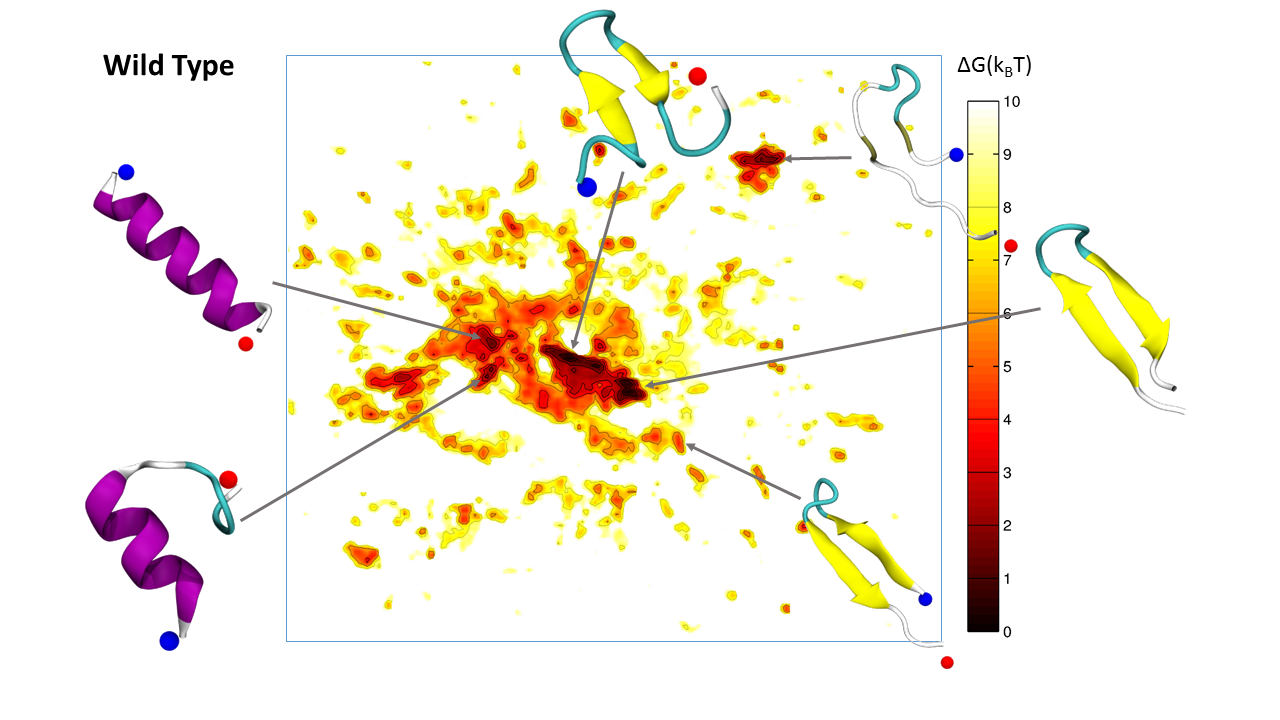
Figure 1: Free energy surface at 299 K for the wild type of the beta hairpin protein as a function of the sketch-map coordinates. The small inset figures show representative structures from each of the minima.

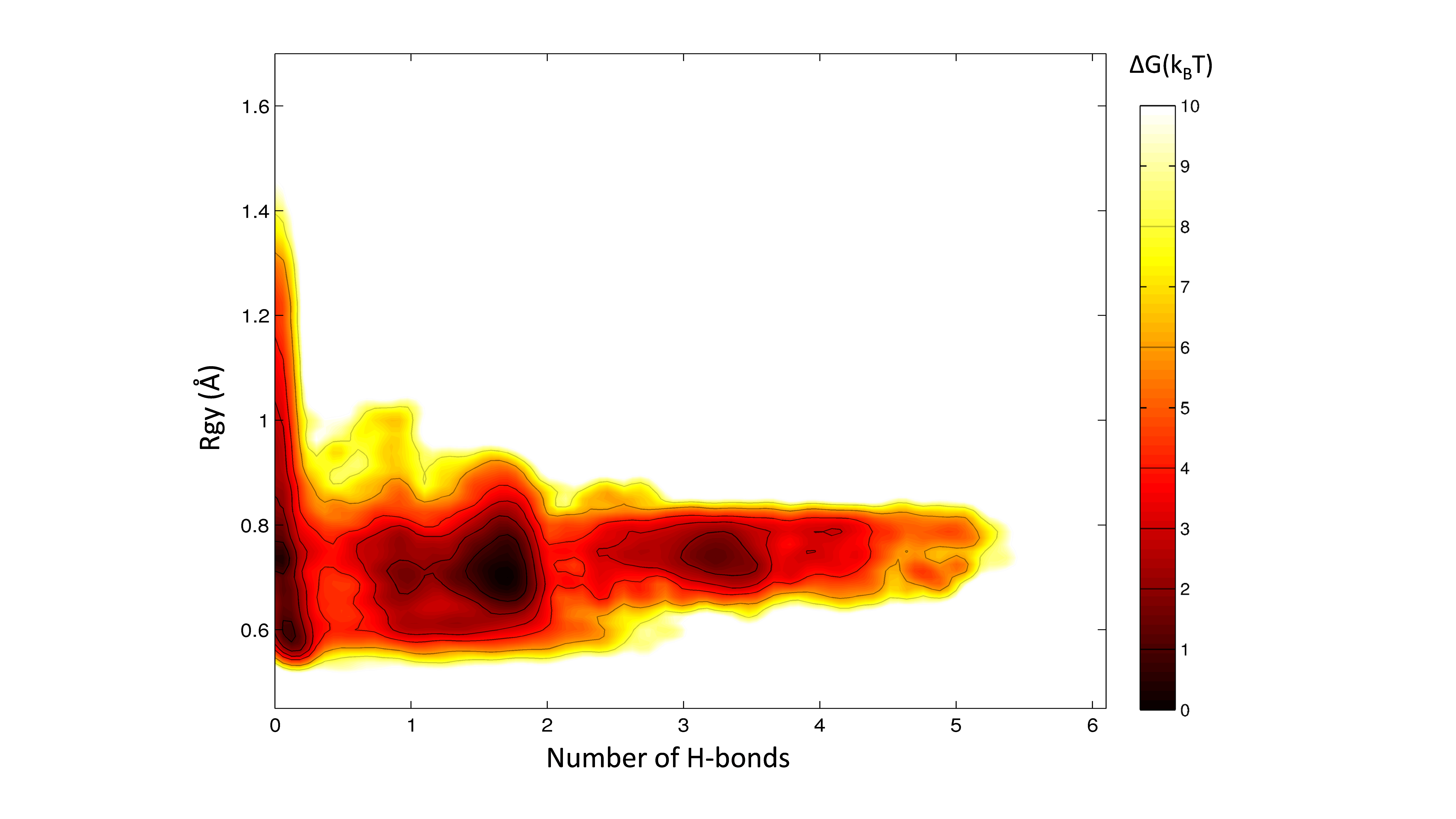
Figure 2: Free energy surface for the wild type protein studied in this work as a function of the number of hydrogen bonds that should be present in the folded configuration and the radius of gyration. The folded state is projected on the right hand side of the figure, misfolded beta hairpin configurations appear in the centre of this figure while all other configurations, including alpha helical ones, are projected on the left hand side of this figure near to the y-axis.

Sketch-map coordinates were generated by selecting 1000 landmark points from our wild-type trajectory using the staged algorithm ²¹ with gamma equal 0.1 and wgamma equal to 1. The set of Ramachandran angles for each protein configuration was used for the high-dimensional, $\mathbf{X}$ vectors in equations 1 and 2 rather than the position of all the atoms as by doing so we eliminate a large amount of redundant information while still providing a good description of the variability in protein structure. Optimal two-dimensional projections for each of the landmark protein configurations were found by minimizing equation 1 with $\sigma=6$, $A=8$, $B=8$, $a=2$ and $b=8$ using the optimization algorithm described in ¹³ . Then, once this initial set of projections was found, the remainder of the trajectory was projected into the sketch-map space using equation 2. so that The free energy surface of the replica at 299.1 K shown in 1 was then constructed by reweighting the histogram generated from our parallel tempering well tempered metadynamics simulations using the method described in ³⁰. There are a number of notable features in 1. Firstly, this figure shows that the free energy surface for the protein is very rough. There are many basins and each of these basins corresponds to a markedly different protein configuration. This behaviour should be compared with that observed in the free energy surface shown in 2, in which the free energy is shown as a function of the radius of gyration and the degree to which the hydrogen bonds that would form in the beta hairpin have formed. Importantly, the coordinate used to measure hydrogen bonding in this second figure is different to that used in the metadynamics simulations. In the metadynamics our measure of the number of backbone atoms is agnostic and simply counts the number of backbone hydrogen bonds that have formed. By contrast, for easy comparison with previous literature, ^{8, 31, 32} in this figure we count only those hydrogen bonds that would be present in the final, folded beta-hairpin configuration.

2 shows a free energy surface that is considerably smoother than that shown in 1. One now sees only three distinct minima in the free energy landscape and many of the basins that were visible in 1 appear to have disappeared. It is therefore apparent that when these commonly-used collective variables are used to analyse the dynamics of the protein one can only really make judgements about the relative stabilities of the folded (beta-hairpin) structure and the unfolded state. However, 1 shows us that multiple configurations, and perhaps more pertinently multiple energetic basins, make up this “unfolded” state. There is incomplete agreement in the literature about what structures together comprise the unfolded ensemble for this protein. While some simulation studies suggest that there is no significant alpha-helical content ³² other see a substantial number of helical configurations^{33, 34, 35}. The free energy surface in 1 seems to suggest that alpha helical configurations are present and that they have free energies that are comparable with those of the beta-hairpin.

Another contentious issue in the literature on this protein concerns the various misfolded configurations that the protein can adopt. Bonomi et al. ³⁶ suggested the existence of one misfolded state. Meanwhile, Best et al. ³⁵ found multiple misfolded configurations, which included Bonomi’s. In our free energy surface we see many of the misfolded configurations that were observed in these studies. We do not see all because in these other studies different force fields were used, which perhaps stabilize different configurations. In our work we used the AMBER99SB-ILDN* ³⁷ because it has been shown to reproduce experimental observations for small peptides and proteins well ³⁸.

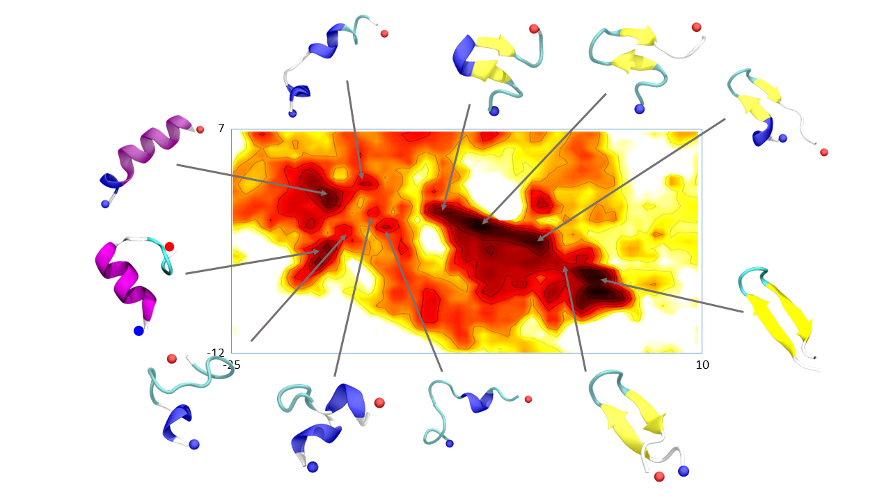
Figure 3: Figure showing the region of the sketch-map projection of the free energy surface containing the beta hairpin and alpha helical configurations. Representative configurations for each of the minima in this region are shown.

3 shows the region of the sketch-map free energy surface around the alpha helical and beta hairpin minima in more detail. This figure shows clearly that there are many minima in the free energy landscape in this region corresponding to structures with various degrees of alpha helical and beta-sheet-like character. The most stable configuration is the folded beta hairpin. However, there are a number of partially folded hairpins that lie relatively close in energy. These configurations have a free energy that is only slightly lower than that of a perfect alpha helix. Most importantly, however, a comparison between figures 1 and 2 clearly shows that variables such as the radius of gyration or the number of native hydrogen bonds, which measure the degree to which the structure resembles that in the folded state, give an incomplete picture of the unfolded state. Alpha-helical configurations appear in a separate basin from the misfolded configurations in 1 but are combined in a single basin in 2.

It is tempting to look for the transition pathways between configurations in these sketch-map coordinates. Care should be taken when doing so, however, as firstly no dynamical information was used in the construction of these coordinates. At best structures appear close together in the projection because they are relatively close together in the high-dimensional space. This does not necessarily mean that the system will rapidly inter-convert between these configurations - two structures that appear close together may well be separated by a substantial energy barrier. Secondly, we have shown ¹⁹ that continuous paths in the high-dimensional space can appear to be discontinuous when projected using sketch-map.

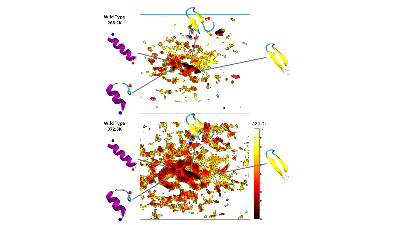
Figure 4: Free energy surfaces for the wild type protein examined in this work as a function of the sketch-map coordinates at temperatures of 268.2 K and 372.3 K. These surfaces were generated by projecting the trajectories for the replicas at these temperatures using a set of landmarks extracted from the trajectory at 299.2 K. As such the various basins in these landscapes can be compared directly with those in 1. The figure shows that at low temperatures the system explores a small part of configuration space and is largely confined to the folded states. At higher temperatures the system explores more of configuration space including a wide variety of unfolded structures. However, this free energy surface tells us that the system will spend a considerable portion of its time in folded configuration even at these relatively high temperatures.

Plotting the free energy surface as a function of the sketch-map variables at a variety of different temperatures using a single reference map obtained at an intermediate temperature is an interesting exercise. When this is done for the trajectories in this work we observe results that are similar to those obtained in a recent work on Lennard-Jones clusters ²¹. 4 shows that at low temperatures the system is confined to the low-energy folded states - the alpha helical and beta sheet configurations. By contrast at higher temperatures the system is free to explore a much wider portion of configuration space including many high energy configurations. It is interesting to note that basins corresponding to the hairpin, the mis-folded hairpin and the helix, are present at all temperatures. In other words, the system spends a substantial amount of time in folded states even when it is at a temperature of 373 K. The apparent stabilities of these folded configurations can be rationalized by noting that the basins corresponding to each of them are wider in the higher temperature free energy surface. It would seem then that increases in entropy that occur because the system fluctuates more wildly about the equilibrium structures at higher temperatures serve to stabilize the folded structure even when the temperature is high. This should be contrasted with the case of small clusters ²¹, where the enthalpic minima appear to be very rigid. In these systems structural fluctuations about these minima appear not to increase strongly with temperature. Consequently, the weights of these enthalpic basins becomes completely irrelevant when the temperature is raised.

3.2 Trpzip4 and D46A mutations

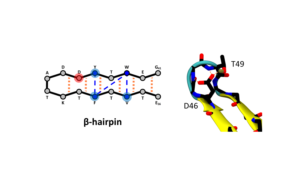
Figure 5: Figure illustrating the mutations we have studied in this work. The left panel shows a schematic of the folded configuration. The red dashed lines indicate the various hydrogen bonds that form between backbone groups in the folded state while the blue dashed lines illustrate the favourable hydrophobic interactions that serve to stabilize the folded state. In the first mutation we examined the residues highlighted in blue were changed to tryptophans. In the second mutation the aspartate residue highlighted in red was changed to an alanine. As shown in the right panel of the figure this aspartate (D46) forms a hydrogen bond to residue T49 in the wild type, which serves to stabilise the loop region for the folded beta hairpin. Alanine cannot form this hydrogen bond and thus this mutation destabilizes the folded state.

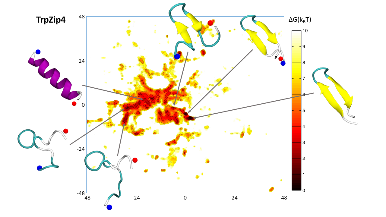
Figure 6: Free energy surface at 299 K for a mutant protein in which residues 45, 52 and 54 have been changed to tryptophans. By comparing this landscape with that of the wild type in 1 it becomes apparent that this mutation serves to stabilize the folded beta hairpin configuration.

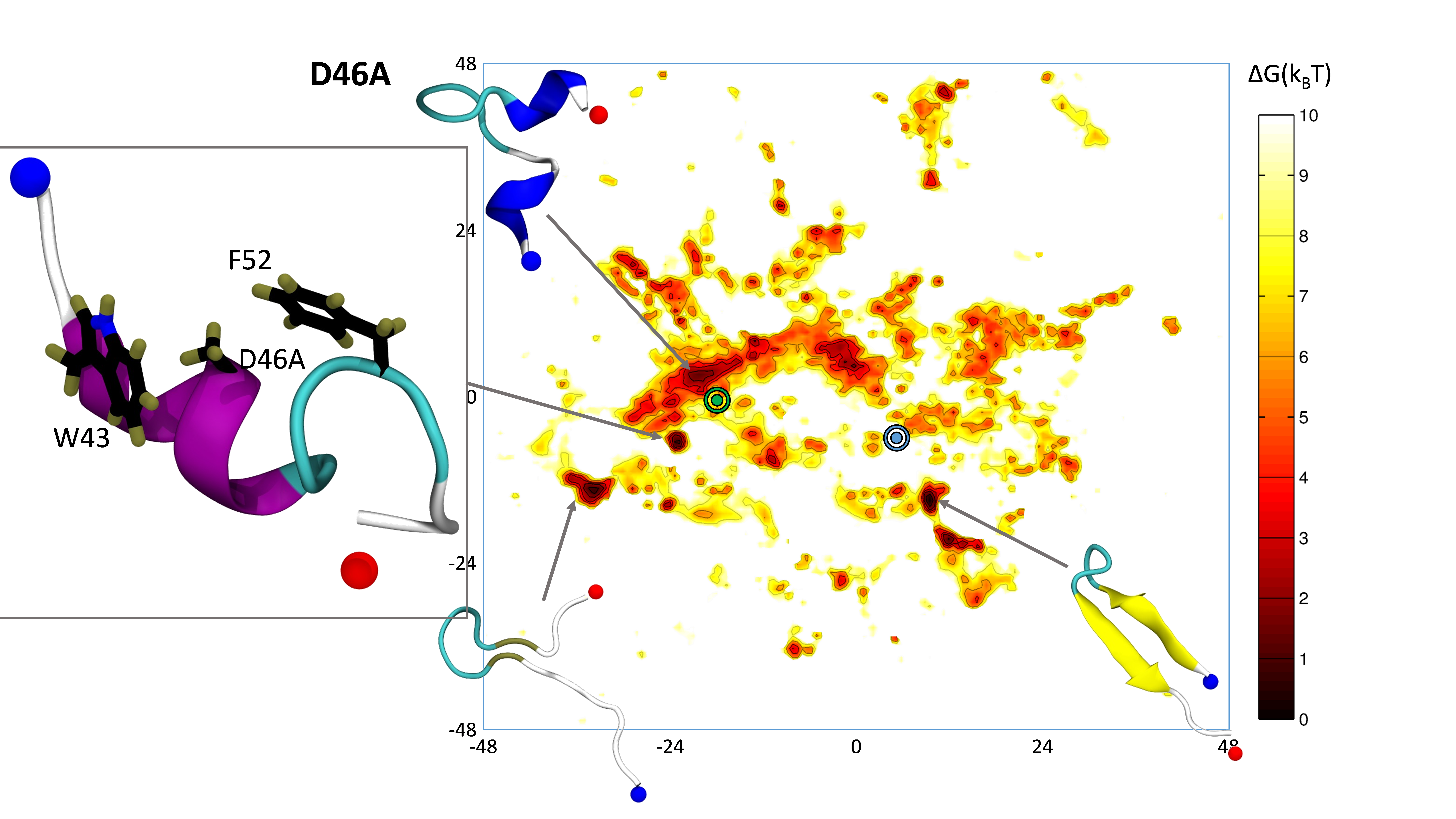
Figure 7: Free energy surface at 299 K for a mutant protein in which residue 46 has been changed into an alanine. The blue and the green markpoints show the position of the folded and the linear alpha helix configurations respectively as observed in the wild type FES. By comparing this landscape with that of the wild type in 1 it becomes apparent that this mutation serves to destabilize the folded beta hairpin configuration as well as the linear alpha helix. As discussed in the text we see from our simulation that the alanine on residue 46, as well as not forming the hydrogen bonds that stabilise the beta hairpin, can also form the hydrophobic contacts shown in the left panel of this figure. This serves to destabilize the linear alpha helix.

It has been suggested that protein energy landscapes always have minima corresponding to the various secondary structural elements as these features in the energy landscape emerge as a result of interactions between the backbone atoms that are unaffected by the amino acid sequence ^{39, 40}. In this view the amino acid sequence only perturbs the energies of this universal library of secondary structure motifs. As a result the sequence, rather than controlling the shape of the funnel that leads to the folded state ⁴¹, serves only to select a folded state from a smörgåsbord of allowable protein configurations. The sketch-map coordinates discussed in the previous section provide us with an interesting opportunity to examine this kind of hypothesis. By projecting the free energy surface for a mutant protein using the sketch-map coordinates that we generated in the previous section for the wild-type protein we can do a basin-by-basin comparison of the free energy landscapes for two proteins with different amino acid sequences. In other words we can examine how the free energy for each of the individual basins in the energy landscape is perturbed by the mutation and can thus perhaps provide more detailed insight than observing simply that one mutation stabilizes the folded state while the other destabilizes it.

With the above experiment in mind we ran parallel-tempering-well-tempered-metadynamics simulations similar to those described at the start of the previous section on two mutations of the beta-hairpin protein. In the first of these mutants we changed the tyrosine, phenylalanine and Valine groups on residues 45, 52 and 54 to tryptophans. The residues we mutated are shown in blue in the left panel of 5. This figure shows that the mutated residues participate in a number of hydrophobic interactions that stabilize the core of the structure. Hence, by making these already hydrophobic residues even more hydrophobic we would expect to further stabilize the folded beta-hairpin configuration ^{42, 43}, which is precisely what is observed in 6. The minima corresponding to the beta-hairpin configuration becomes deeper as do the satellite basins around it that correspond to the various partially unfolded configurations of this structure.

6 shows that the free energy difference between the perfect-alpha helix structure and the folded beta hairpin is larger for this mutated protein than it is in the wild type. Even so the alpha-helix still has a reasonably low free energy so the system would still expect to spend a considerable fraction of its time in alpha helical configurations. The reason for this is probably connected to the fact that alpha helices are held together by backbone hydrogen bonds between carboxylate and amine groups that are four residues apart on the protein chain. A mutation of the protein would not be expected to change the strength of these particular interactions significantly. A significant change in the hydrophobicity of the amino acid side chains might, by contrast, act to destabilize the alpha helix because, in an alpha helix, all the side chains are exposed to the solvent. It would seem from 6, however, that making hydrophobic residues slightly more hydrophobic does not perturb the free energy landscape greatly enough to bring about this change.

In the second mutation we substituted the aspartate on position 46, which is shown in red in the left panel of 5, for an alanine. As shown in the right panel of 5 in the wild-type this aspartate stabilises the loop region of the folded state by forming hydrogen bonds both to the backbone amide nitrogens of those residues in the loop and to the side-chain of threonine 49. Alanine will not form these hydrogen bonds, which explains why there is no longer a basin corresponding to the beta-hairpin structure or any satellite basins corresponding to partially-unfolded beta hairpins in the free energy landscape for this mutant (see 7). Interestingly, this mutation also appears to affect the stability of the perfect alpha-helix. The linear alpha-helical configuration that appears in 1 and 6 is not shown in 7 because the system did not visit this particular configuration in our parallel tempering simulations on the D46A mutant. This fact is evidenced in the free energy surfaces shown in figures 1, 6 and 7. In the first two of these free energy surfaces the linear alpha helix is shown to correspond to a rather distinctive sausage-shaped basin in the free energy landscape, which is no longer visible in 7. To be clear, it is not that this mutant does not visit alpha helices at all it is rather that the alpha helical configurations it does visit are folded back on themselves (see the left panel of 7). One explanation for this is that by substituting the aspartate on residue 46 with an alanine we have made a formerly hydrophilic residue hydrophobic. As discussed previously, this would destabilize the alpha helix as in this configuration all the side chains are exposed to the solvent. In addition, the left panel of 7 show that this mutated alanine group forms two hydrophobic contacts that stabilise a bent alpha helix over the linear one.

As discussed previously the global minimum for both the wild-type and the TrpZip4 mutant is a beta hairpin configuration. There is no basin corresponding to this structure in the D46A free energy surface for the reasons discussed in the previous paragraph. However, this is not to say that beta hairpins do not form for this particular amino acid sequence. There is a prominent basin that corresponds to a structure in which an anti parallel beta hairpin has formed and in which the loop is between residues 44 and 47 in the bottom right hand corner of the free energy surface shown in 7. This structure is favourable because within it there are numerous hydrophobic contacts. Furthermore, it appears in the free energy landscapes for both the wild-type and TrpZip4 mutant. However, in those proteins the feature in the free energy landscape corresponding to this structure is considerably less prominent because this structure contains fewer hydrophobic contacts than the perfect beta hairpin. The reason it is so prominent for the D46A is almost certainly connected to the fact that it is unfavourable to form the loop between residues 47 and 51 because the (mutated) alanine group on residue 46 cannot form the prerequisite hydrogen bonds.

4 Conclusion

The sketch-map coordinates that have been used to analyse the long MD trajectories generated in this study have shown themselves to be a useful tool. When the free energy surface is displayed as a function of these bespoke coordinates one can see the wide range of configurations adopted by a particular chemical system. For proteins this means that one can use sketch-map coordinates to view, basin by basin, how a change in the conditions or a change in the amino acid sequence affects the free energy landscape of a protein. This is useful as evidence keeps emerging that denaturants such as urea ³¹ work by changing the relative free energy of unfolded configurations. Similarly a better understanding of how the free energy landscapes of proteins change in response to experimental conditions will allow us to better understand phenomena such as the Hoffmeister series ⁴⁴ or even how changing the forcefield parameters changes the way phase space is sampled. Lastly, there is increasing evidence that so called intrinsically disordered proteins play an important role in biology. Many of these proteins undergo folding and binding at the same time and hence untangling their modus operandi requires a detailed view on how free energies of folding are perturbed by binding and vice versa.

Our results suggest that mutations can stabilize or destabilize particular configurations of the peptide by either allowing it to form new energetically-favourable contacts or by preventing them from forming particular native contacts. It seems reasonable to suppose that this may well be valid for other small, isolated proteins so our results would appear to support backbone theories ^{39, 40} of protein folding more than they support those theories based on the amino acids sequence sculpting the folding funnel ⁴⁵. However, in a bigger protein regions of secondary structure are likely to be stabilized by additional interactions that will all serve to ensure that the protein adopts its biologically-active, tertiary structure. In these proteins the tertiary structure is thus less likely to be affected by small (point) mutations. As such further study is thus certainly required if we are to determine the effect mutations have on the folding landscape in general terms.

We were able to come to these conclusions because sketch-map coordinates allow one to perform an unbiased analysis of the simulation results. Additionally, equation 2 ensures that we can calculate projections easily for any vector of 30 torsional angles. We can even use these coordinates to enhance sampling and to thus drive the system to explore high energy parts of configuration space ¹⁹. All the evidence we have accumulated thus far further suggests that this procedure will produce sensible projections. We thus have coordinates that can be used for a number of different amino acid sequences and which are not constructed based on previous knowledge on the structure of the folded state. In short, we are in a position where we can compare data collected from multiple trajectories and where our previous understanding does not limit our analysis. As such there is thus a greater chance of discovering unexpected or surprising results.

5 Acknowledgements

The authors would like to thank CSCS for computer time and also acknowledge funding from the European Union (Grant ERC-2009-AdG-24707). AA was supported by an EMBO long-term fellowship.

References

- Lodish et al. 2003 Lodish, H.; Berk, A.; Matsudaira, P.; Kaiser, C. A.; Krieger, M.; Scott, M. P.; Zipursky, S. L.; Darnell, J. Molecular Cell Biology, Fifth ed.; W H Freeman: New York, 2003
- Dunker et al. 2008 Dunker, A. K.; Silman, I.; Uversky, V. N.; Sussman, J. L. Curr. Opin. Struct. Biol. 2008, 18, 756–764
- Christopoulos 2002 Christopoulos, A. Nat. Rev. Drug Discovery 2002, 1, 198–210
- Dyson and Wright 2005 Dyson, H. J.; Wright, P. E. Nat. Rev. Mol. Cell Biol. 2005, 6, 197–208
- Shaw et al. 2010 Shaw, D. E.; Maragakis, P.; Lindorff-Larsen, K.; Piana, S.; Dror, R. O.; Eastwood, M. P.; Bank, J. A.; Jumper, J. M.; Salmon, J. K.; Shan, Y.; Wriggers, W. Atomic-Level Characterization of the Structural Dynamics of Proteins. Science 2010, 330, 341–346
- Li and Cirino 2014 Li, Y.; Cirino, P. C. Recent advances in engineering proteins for biocatalysis. Biotechnol. Bioeng. 2014, 111, 1273–1287
- Bouvignies et al. 2011 Bouvignies, G.; Vallurupalli, P.; Hansen, D. F.; Correia, B. E.; Lange, O.; Bah, A.; Vernon, R. M.; Dahlquist, F. W.; Baker, D.; Kay, L. E. Solution structure of a minor and transiently formed state of a T4 lysozyme mutant. Nature 2011, 477, 111–U134
- Bussi et al. 2006 Bussi, G.; Gervasio, F. L.; Laio, A.; Parrinello, M. Free-Energy Landscape for Hairpin Folding from Combined Parallel Tempering and Metadynamics. J. Chem. Am. Soc. 2006, 128, 13435–13441, PMID: 17031956
- Gnanakaran et al. 2003 Gnanakaran, S.; Nymeyer, H.; Portman, J.; Sanbonmatsu, K. Y.; Garcia, A. E. Peptide folding simulations. Curr. Opin. Struct. Biol. 2003, 13, 168 – 174
- Weinstock et al. 2007 Weinstock, D. S.; Narayanan, C.; Felts, A. K.; Andrec, M.; Levy, R. M.; Wu, K.-P.; Baum, J. Distinguishing among Structural Ensembles of the GB1 Peptide: REMD Simulations and NMR Experiments. J. Am. Chem. Soc. 2007, 129, 4858–4859, PMID: 17402734
- Deighan et al. 2012 Deighan, M.; Bonomi, M.; Pfaendtner, J. Efficient Simulation of Explicitly Solvated Proteins in the Well-Tempered Ensemble. J. Chem. Theory Comput. 2012, 8, 2189–2192
- Zuckerman 2011 Zuckerman, D. M. Equilibrium Sampling in Biomolecular Simulations. Annual Review of Biophysics 2011, 40, 41–62, PMID: 21370970
- Ceriotti et al. 2011 Ceriotti, M.; Tribello, G. A.; Parrinello, M. Simplifying the representation of complex free-energy landscapes using sketch-map. Proc. Natl. Acad. Sci. USA 2011, 108, 13023–13029
- Tenenbaum et al. 2000 Tenenbaum, J. B.; Silva, V. d.; Langford, J. C. A Global Geometric Framework for Nonlinear Dimensionality Reduction. Science 2000, 290, 2319–2323
- Roweis and Saul 2000 Roweis, S. T.; Saul, L. K. Nonlinear Dimensionality Reduction by Locally Linear Embedding. Science 2000, 290, 2323–2326
- Coifman et al. 2005 Coifman, R. R.; Lafon, S.; Lee, A. B.; Maggioni, M.; Nadler, B.; Warner, F.; Zucker, S. W. Geometric diffusions as a tool for harmonic analysis and structure definition of data: Multiscale methods. Proc. Natl. Acad. Sci. USA of the United States of America 2005, 102, 7432–7437
- Coifman and Lafon 2006 Coifman, R. R.; Lafon, S. Diffusion maps. Appl. Comput. Harmon. Anal. 2006, 21, 5 – 30
- Belkin and Niyogi 2003 Belkin, M.; Niyogi, P. Laplacian Eigenmaps for Dimensionality Reduction and Data Representation. Neural Comput. 2003, 15, 1373–1396
- Tribello et al. 2012 Tribello, G. A.; Ceriotti, M.; Parrinello, M. Using sketch-map coordinates to analyze and bias molecular dynamics simulations. Proc. Natl. Acad. Sci. USA 2012, 109, 5196–5201
- Cox and Cox 1994 Cox, T. F.; Cox, M. A. A. Multidimensional Scaling; London: Chapman and Hall, 1994
- Ceriotti et al. 2013 Ceriotti, M.; Tribello, G. A.; Parrinello, M. Demonstrating the Transferability and the Descriptive Power of Sketch-Map. J. Chem. Theory Comput. 2013, 9, 1521–1532
- Blanco et al. 1994 Blanco, F. J.; Rivas, G.; Serrano, L. Nat. Struct. Biol. 1994, 1, 584–590
- Hughes and Waters 2006 Hughes, R.; Waters, M. Curr. Opin. Struct. Biol. 2006, 16, 514–524
- Muñoz et al. 1997 Muñoz, V.; Thompson, P.; Hofrichter, J.; Easton, W. Nature 1997, 390, 196–199
- Hess et al. 2008 Hess, B.; Kutzner, C.; van der Spoel, D.; Lindahl, E. GROMACS 4: Algorithms for highly efficient, load-balanced and scalable molecular simulation. J. Chem. Theory Comput. 2008, 4, 435–447
- Laio and Parrinello 2002 Laio, A.; Parrinello, M. Escaping free-energy minima. Proc. Natl. Acad. Sci. USA 2002, 99, 12562–12566
- Bonomi and Parrinello 2010 Bonomi, M.; Parrinello, M. Enhanced Sampling in the Well-Tempered Ensemble. Phys. Rev. Lett. 2010, 104, 190601
- Bonomi et al. 2009 Bonomi, M.; Branduardi, D.; Bussi, G.; Camilloni, C.; Provasi, D.; Raiteri, P.; Donadio, D.; Marinelli, F.; Pietrucci, F.; Broglia, R. A.; Parrinello, M. PLUMED: A portable plugin for free-energy calculations with molecular dynamics. Comp. Phys. Comm. 2009, 180, 1961 – 1972
- Tribello et al. 2014 Tribello, G. A.; Bonomi, M.; Branduardi, D.; Camilloni, C.; Bussi, G. {PLUMED} 2: New feathers for an old bird. Comput. Phys. Commun. 2014, 185, 604 – 613
- Bonomi et al. 2009 Bonomi, M.; Barducci, A.; Parrinello, M. Reconstructing the equilibrium Boltzmann distribution from well-tempered metadynamics. J. Comput. Chem. 2009, 30, 1615–1621
- Berteotti et al. 2011 Berteotti, A.; Barducci, A.; Parrinello, M. Effect of Urea on the -Hairpin Conformational Ensemble and Protein Denaturation Mechanism. J. Am. Chem. Soc. 2011, 133, 17200–17206
- Zhou et al. 2001 Zhou, R.; Berne, B.; Germain, R. The free energy landscape for beta hairpin folding in explicit water. Proc. Natl. Acad. Sci. U.S.A. 2001, 98, 14931–14936
- Best and Mittal 2011 Best, R. B.; Mittal, J. Microscopic events in beta-hairpin folding from alternative unfolded ensembles. Proc. Natl. Acad. Sci. U.S.A. 2011, 108, 11087–11092
- Garcia and Sanbonmatsu 2001 Garcia, A.; Sanbonmatsu, K. Exploring the energy landscape of a beta hairpin in explicit solvent. Proteins: Struct., Funct., Genet. 2001, 42, 345–354
- De Sancho et al. 2013 De Sancho, D.; Mittal, J.; Best, R. B. Folding Kinetics and Unfolded State Dynamics of the GB1 Hairpin from Molecular Simulation. J. Chem. Theory Comput. 2013, 9, 1743–1753
- Bonomi et al. 2008 Bonomi, M.; Branduardi, D.; Gervasio, F. L.; Parrinello, M. The Unfolded Ensemble and Folding Mechanism of the C-Terminal GB1 -Hairpin. J. Am. Chem. Soc. 2008, 130, 13938–13944
- Lindorff-Larsen et al. 2010 Lindorff-Larsen, K.; Piana, S.; Palmo, K.; Maragakis, P.; Klepeis, J. L.; Dror, R. O.; Shaw, D. E. Improved side-chain torsion potentials for the Amber ff99SB protein force field. Proteins: Struct., Funct., Bioinf. 2010, 78, 1950–1958
- Lindorff-Larsen et al. 2012 Lindorff-Larsen, K.; Maragakis, P.; Piana, S.; Eastwood, M. P.; Dror, R. O.; Shaw, D. E. Systematic Validation of Protein Force Fields against Experimental Data. PLoS ONE 2012, 7, e32131
- Rose et al. 2006 Rose, G. D.; Fleming, P. J.; Banavar, J. R.; Maritan, A. Proc. Nat. Sci U.S.A. 2006, 103, 16623
- Hegler et al. 2008 Hegler, J. A.; Weinkam, P.; Wolynes, P. G. HFSP Journal 2008, 2, 307
- Hegler et al. 2008 Hegler, J. A.; Weinkam, P.; Wolynes, P. G. HFSP Journal 2008, 2, 307
- Noy et al. 2008 Noy, K.; Kalisman, N.; Keasar, C. Prediction of structural stability of short beta-hairpin peptides by molecular dynamics and knowledge-based potentials. BMC Struct. Biol. 2008, 8
- Juraszek and Bolhuis 2009 Juraszek, J.; Bolhuis, P. G. Effects of a Mutation on the Folding Mechanism of beta-Hairpin. J. Phys. Chem. B 2009, 113, 16184–16196
- F.Hofmeister 1888 F.Hofmeister, Arch. Exp. Pathol. Pharmacol. 1888, 24, 247–260
- Oliverberg and Wolynes 2008 Oliverberg, M.; Wolynes, P. G. Quaterly Reviews of Biophyics 2008, 71, 245