Greeks’ pitfalls for the COS method in the Laplace model

Abstract

The Greeks Delta, Gamma and Speed are the first, second and third derivatives of a European option with respect to the current price of the underlying asset. The Fourier cosine series expansion method (COS method) is a numerical method for approximating the price and the Greeks of European options. We develop a closed-form expression of Speed for various European options in the Laplace model and we provide sufficient conditions for the COS method to approximate Speed. We show empirically that the COS method may produce numerically nonsensical results if theses sufficient conditions are not met.
Keywords: Laplace model, Greeks, Gamma, Speed, COS method, mispricing
JEL classification: G10 G13 C63

1 Introduction

Financial contingent claims like European options are widely used by financial institutions. The derivatives or sensitives of options are important parameters for hedging and risk management purposes and are also called Greeks. The most important Greeks are Delta and Gamma, which are the first and second derivatives of a European option with respect to the current price of the underlying asset.

The third derivative of an option with respect to the underlying asset is called Speed. As observed by Haug (2006, p. 36), Speed plays an important role: “A high Speed value indicates that the Gamma is very sensitive to moves in the underlying asset. […] For an option trader […] it can definitely make sense to have a sense of an option’s Speed.” Speed appears frequently in the literature, see e.g., Taleb (1997, p.194); Garman (1992); Fouque et al. (2000).

A numerically efficient way to compute prices and Greeks of a European option is the COS method, which is widely used in mathematical finance; see Fang and Oosterlee (2009b, 2011); Grzelak and Oosterlee (2011); Ruijter and Oosterlee (2012); Zhang and Oosterlee (2013); Ruijter et al. (2015, Section 2.2.1); Leitao et al. (2018); Liu et al. (2019a, b); Oosterlee and Grzelak (2019); Bardgett et al. (2019); Junike and Pankrashkin (2022).

See Junike (2023, Thm. 5.6) for sufficient conditions on the density of the log-returns to ensure that the COS method is able to approximate the Greeks Delta and Gamma. A sufficient condition is provided if the density of the log-returns of the underlying asset is smooth.

This article deals mainly with the Laplace model, which was introduced by Madan (2016). It is a special case of the Variance Gamma model; see Madan et al. (1998); which in turn is implemented in Quantlib, a software package widely used in the finance industry.

We make the following main contributions: We prove a new formula for the COS method to approximate Speed. Further, we develop new formulas for the Greeks Gamma and Speed of European plain vanilla put and call options and digital options in the Laplace model. We correct an existing formula in the literature for Gamma.

The Gamma of a digital option in the Laplace model has a jump. Therefore, the derivative of Gamma, i.e., Speed, does not exist as a classical function. One could however, define Speed as a pointwise derivative of Gamma. Then Speed exists, except at the point where Gamma jumps.

The existing formulas in the literature on the COS method to approximate the Greeks of an option can always be implemented. However, as another contribution, we show empirically that the COS method is not able to approximate the Greek Speed of a digital option in any sense. For Speed in the Laplace model, the COS method produces only meaningless results. This behavior of the COS method can partially be explained by the fact that the density of the log-returns in the Laplace model is not differentiable and hence does not satisfy the assumptions in Theorem 5.6 in Junike (2023). It certainly shows that one has to be very careful when implementing the COS method. One should not blindly trust the output of the COS method without first verifying the conditions to apply the method.

This article is structured as follows: In Section 2 we briefly recall the COS method from the literature and provide sufficient conditions under which Speed can be approximated numerically using the COS method. In Section 3, we recall formulas of the price and Delta of European options within the Laplace model from the literature and deduce new formulas for Gamma and Speed. In Section 4, we show empirically that the COS method produces numerically nonsensical results for the Speed of a digital option. Section 5 concludes.

2 COS method

We consider an investor with time horizon $T>0$. We assume that there is a financial market consisting of a stock with price $S_{0}>0$ today and (random) price

$$S_{T}=S_{0}\bar{S}$$ (1)

at the end of the time horizon, where $\bar{S}$ is a random variable that does not depend on $S_{0}$. Equation (1) holds for many models, e.g., those of Heston (1993) and Bates (1996) as well as the Lévy models; see Schoutens (2003). We assume that there is a bank account paying continuous compound interest $r\in\mathbb{R}$ and we assume that the market is arbitrage-free; we denote by $Q$ the risk-neutral measure. All expectations are taken under $Q$.

There is a European option with maturity $T>0$ and payoff $g(S_{T})$ at $T$, where $g:[0,\infty)\to\mathbb{R}$. In particular, we consider plain vanilla call and put options and digital options. Let $\eta:=E[\log(S_{T})]-\log(S_{0})$. Then $\eta$ does not depend on $S_{0}$ by Equation (1). As in Junike (2023, Section 5), we define

$$v(x,s):=e^{-rT}g(\exp(x+\log(s)+\eta)),\quad x\in\mathbb{R},\quad s>0.$$ (2)

The price of the European option is then given by

$$e^{-rT}E[g(S_{T})] =\int_{\mathbb{R}}v(x,S_{0})f(x)dx,$$ (3)

where $f$ is the density of the centralized log-returns $X:=\log(S_{T})-E[\log(S_{T})]$.

The integral at the right-hand side of Equation (3) can be numerically solved by the COS method if the characteristic function $\varphi$ of $f$ is given in closed form. This is the case for many financial models; see for instance Fang and Oosterlee (2009a) and the references therein.

We use the following notation to describe the COS method: By $f^{(j)}$ we denote the $j^{th}$-derivative of $f$. We use the convention $f^{(0)}\equiv f$. By $\left\|.\right\|_{\infty}$ we denote the supremum norm, i.e., $\left\|f\right\|_{\infty}=\sup_{x\in\mathbb{R}}f(x)$. Let $\mu_{n}$ be the $n^{th}-$moment of $f$, i.e., $\mu_{n}=\int_{\mathbb{R}}x^{n}f(x)dx$. The $n^{th}-$moment can be obtained from $\varphi$ by

$$\mu_{n}=\frac{1}{i^{n}}\left.\frac{\partial^{n}}{\partial u^{n}}\varphi(u)\right|_{u=0}.$$

Let $L>0$. By

$$v_{k}:=\int_{-L}^{L}v(x,S_{0})\cos\left(k\pi\frac{x+L}{2L}\right)dx,\quad k=0,1,...,$$

we denote the Cosine-Fourier coefficients of the function $v$. We further define

$$c_{k}^{j} =\frac{1}{L}\Re\bigg{\{}\bigg{(}-i\frac{k\pi}{2L}\bigg{)}^{j}\varphi\bigg{(}\frac{k\pi}{2L}\bigg{)}e^{i\frac{k\pi}{2}}\bigg{\}},\quad k=0,1,...,\quad j=0,...,3.$$ (4)

As in Junike (2023), we make the following technical assumptions:

Assumption A1.

Let $J\geq 4$. We assume that $f$ is bounded, $(J+1)$-times continuously differentiable, with bounded derivatives.

Assumption A2.

We assume that there are some $C_{1},C_{2},L_{0}>0$ such that

$$|f^{(j)}(x)|\leq C_{1}C_{2}^{j}e^{-C_{2}|x|},\quad j=0,...,J+1,\quad|x|\geq L_{0}.$$ (5)

The following Theorem provides sufficient conditions to approximate the price and the Greeks Delta, Gamma and Speed numerically using the COS method.

Theorem 1.

Let Assumptions A1 and A2 be in force. Let $\varepsilon>0$ be sufficiently small. Let $\gamma=\min\big{\{}\varepsilon,\varepsilon S_{0},\frac{\varepsilon S_{0}^{2}}{2},\frac{\varepsilon S_{0}^{3}}{6}\big{\}}$. Let $g:[0,\infty)\to\mathbb{R}$ be bounded. Let $v$ be defined as in Equation (2). For some even $n\in\mathbb{N}$, define

$$L=\sqrt[n]{\frac{2K\mu_{n}}{\gamma}}$$ (6)

and $\xi=\sqrt{2L}K$. Let $k\in\{1,...,J-3\}$ and

$$N \geq\left(\frac{2^{k+2}\left(\max_{\ell\in\{0,1,2,3\}}\left\|f^{(k+1+\ell)}\right\|_{\infty}\right)L^{k+\frac{3}{2}}}{k\pi^{k+1}}\frac{12\xi}{\gamma}\right)^{\frac{1}{k}}.$$ (7)

It follows that the price and the Greeks Delta, Gamma and Speed can be approximated by finite sums as follows:

$$\bigg{|}\int_{\mathbb{R}}v(x,S_{0})f(x)dx-\sum_{k=0}^{N}{}^{\prime}c_{k}^{0}v_{k}\bigg{|}\leq\varepsilon,$$

$$\bigg{|}\frac{\partial}{\partial S_{0}}\int_{\mathbb{R}}v(x,S_{0})f(x)dx-\bigg{(}-\frac{1}{S_{0}}\sum_{k=0}^{N}{}^{\prime}c_{k}^{1}v_{k}\bigg{)}\bigg{|}\leq\varepsilon,$$

$$\bigg{|}\frac{\partial^{2}}{\partial S_{0}^{2}}\int_{\mathbb{R}}v(x,S_{0})f(x)dx-\frac{1}{S_{0}^{2}}\sum_{k=0}^{N}{}^{\prime}(c_{k}^{1}+c_{k}^{2})v_{k}\bigg{|}\leq\varepsilon,$$

$$\bigg{|}\frac{\partial^{3}}{\partial S_{0}^{3}}\int_{\mathbb{R}}v(x,S_{0})f(x)dx-\bigg{(}-\frac{1}{S_{0}^{3}}\sum_{k=0}^{N}{}^{\prime}(2c_{k}^{1}+3c_{k}^{2}+c_{k}^{3})v_{k}\bigg{)}\bigg{|}\leq\varepsilon,$$

where $\sum{}^{\prime}$ indicates that the first summand (with $k=0$) is weighted by one-half.

Proof.

The formulas for the price, Delta and Gamma follow from Junike (2023, Thm. 5.2). We proof the formula for Speed. As in the proof of Lemma 5.1 in Junike (2023), one can show by interchanging differentiation and integration that

$$\frac{\partial^{3}}{\partial S_{0}^{3}}\int_{\mathbb{R}}v(x,S_{0})f(x)dx=-\frac{1}{S_{0}^{3}}\int_{\mathbb{R}}v(x,S_{0})\big{(}2f^{(1)}(x)+3f^{(2)}(x)+f^{(3)}(x)\big{)}dx.$$

It follows by Junike (2023, Thm. 3.8) that

$$\bigg{|}\frac{\partial^{3}}{\partial S_{0}^{3}}\int_{\mathbb{R}}v(x,S_{0})f(x)dx -\bigg{(}-\frac{1}{S_{0}^{3}}\sum_{k=0}^{N}{}^{\prime}(2c_{k}^{1}+3c_{k}^{2}+c_{k}^{3})v_{k}\bigg{)}\bigg{|}$$

$$= \frac{1}{S_{0}^{3}}\bigg{|}\int_{\mathbb{R}}v(x,S_{0})\big{(}2f^{(1)}(x)+3f^{(2)}(x)+f^{(3)}(x)\big{)}dx$$

$$-\sum_{k=0}^{N}{}^{\prime}(2c_{k}^{1}+3c_{k}^{2}+c_{k}^{3})v_{k}\bigg{|}$$

$$\leq \frac{2}{S_{0}^{3}}\bigg{|}\int_{\mathbb{R}}v(x,S_{0})f^{(1)}(x)-\sum_{k=0}^{N}{}^{\prime}c_{k}^{1}v_{k}\bigg{|}$$

$$+\frac{3}{S_{0}^{3}}\bigg{|}\int_{\mathbb{R}}v(x,S_{0})f^{(2)}(x)-\sum_{k=0}^{N}{}^{\prime}c_{k}^{2}v_{k}\bigg{|}$$

$$+\frac{1}{S_{0}^{3}}\bigg{|}\int_{\mathbb{R}}v(x,S_{0})f^{(3)}(x)-\sum_{k=0}^{N}{}^{\prime}c_{k}^{3}v_{k}\bigg{|}$$

$$\leq \frac{6\gamma}{S_{0}^{3}}\leq\varepsilon,$$

which concludes the proof. ∎

Remark 2.

The COS method is a very efficient way to compute prices and Greeks because the coefficients $c_{k}^{j}$ can be obtained directly if $\varphi$ is given in closed form and the coefficients $v_{k}$ can also be computed explicitly for plain vanilla European options and European digital options, see Fang and Oosterlee (2009a); Junike and Pankrashkin (2022).

3 Greeks under the Laplace model

In the Laplace model, the log-returns are described by a Laplace-distributed random variable; see Madan (2016). The Laplace model is a special case of the Variance Gamma model; see Madan et al. (1998). The stock price at time $T>0$ is defined by

$$S_{T}=S_{0}\exp\left((r-q)T+X+\log\left(1-\frac{\sigma^{2}T}{2}\right)\right),$$

where $r$ is the risk-free interest rate, $q$ is a dividend yield and $\sigma>0$ is a free parameter. $X$ is Laplace distributed with mean zero and standard deviation $\sigma\sqrt{T}$ and has density

$$f_{\text{Lap}}(x)=\frac{1}{\sigma\sqrt{2T}}e^{\frac{-\sqrt{2}|x|}{\sigma\sqrt{T}}},\quad-\infty<x<\infty.$$ (8)

The centralized log-returns are equal to $X$. The characteristic function of $X$ is given explicitly by

$$\varphi(u) =\frac{1}{\left(1+\frac{u^{2}\sigma^{2}T}{2}\right)},\quad u\in\mathbb{R}.$$

$f_{\text{Lap}}$ satisfies Assumption A2, see Junike (2023, Example 3.4), and is infinitely many times differentiable on $\mathbb{R}\setminus\{0\}$. However, $f_{\text{Lap}}$ is not differentiable a zero and hence does not satisfy Assumption A1. As in Madan (2016), let

$$d:=d(S_{0}):=\frac{\log(\frac{K}{S_{0}})}{\sigma\sqrt{T}}-\frac{r-q}{\sigma}\sqrt{T}-\frac{\log(1-\frac{\sigma^{2}T}{2})}{\sigma\sqrt{T}},\quad S_{0}>0.$$

In Madan (2016) and Madan et al. (2017), the price, Delta and Gamma of European plain vanilla options are determined. Madan et al. (2017) claim that Gamma is discontinuous as a function of $S_{0}$ if $d=0$. However, as shown by Proposition 5, Gamma is a continuous function of $S_{0}$ for all $S_{0}>0$. This is also confirmed empirically by Figure 1. In the following propositions, we recall the formulas for the price and Delta of a European plain vanilla option and we provide new formulas for Gamma and Speed. Further, we derive formulas for the price, Delta, Gamma and Speed of a digital option. Figure 1 shows the price, Delta, Gamma and Speed of a plain vanilla put option in closed form and the approximations using the COS method.

Proposition 3.

The prices of plain vanilla put and call options are given by

$$P(S_{0})=\frac{1}{2}Ke^{-rT}e^{-\sqrt{2}|d|}-\frac{1}{2}S_{0}e^{-qT}e^{-(\sqrt{2}+\sigma\sqrt{T})|d|}(1-\frac{\sigma\sqrt{T}}{\sqrt{2}})\quad,d\leq 0$$

$$C(S_{0})=S_{0}e^{-qT}\frac{e^{-(\sqrt{2}-\sigma\sqrt{T})|d|}}{2}(1+\frac{\sigma\sqrt{T}}{\sqrt{2}})-Ke^{-rT}\frac{e^{-\sqrt{2}|d|}}{2}\quad,d\geq 0$$

$$P(S_{0})=C(S_{0})+Ke^{-rT}-S_{0}e^{-qT}\quad,d\geq 0$$

$$C(S_{0})=P(S_{0})+S_{0}e^{-qT}-Ke^{-rT}\quad,d\leq 0.$$

Proof.

See Madan (2016). ∎

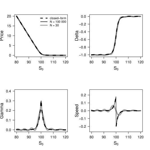
Figure 1: Price, Delta, Gamma and Speed of a put option with parameters $K=100$, $r=0$, $T=0.2$ and $\sigma=0.05$ as a function of $S_{0}$ and approximations using the COS method for various values for $N$. Here, $d=0\Leftrightarrow S_{0}=100.025$. For the COS method, we set $\varepsilon=10^{-5}$ and use $n=8$ moments to obtain $L=0.5$ by Equation (6).

Proposition 4.

The Delta of a European plain vanilla put option is given by

$$\Delta_{Put}(S_{0})=\begin{cases}-\frac{1}{2}e^{-qT}e^{(\sqrt{2}+\sigma\sqrt{T})d}(1-\frac{\sigma\sqrt{T}}{\sqrt{2}})&,d\leq 0\\ \frac{1}{2}e^{-qT}e^{-(\sqrt{2}-\sigma\sqrt{T})d}(1+\frac{\sigma\sqrt{T}}{\sqrt{2}})-e^{-qT}&,d\geq 0.\end{cases}$$

Delta of a European plain vanilla call option is given by

$$\Delta_{Call}(S_{0})=\begin{cases}-\frac{1}{2}e^{-qT}e^{(\sqrt{2}+\sigma\sqrt{T})d}(1-\frac{\sigma\sqrt{T}}{\sqrt{2}})+e^{-qT}&,d\leq 0\\ \frac{1}{2}e^{-qT}e^{-(\sqrt{2}-\sigma\sqrt{T})d}(1+\frac{\sigma\sqrt{T}}{\sqrt{2}})&,d\geq 0.\end{cases}$$

Proof.

See Madan (2016). ∎

Proposition 5.

The Gamma of a European plain vanilla put or call option is given by

$$\Gamma_{Put}(S_{0})=\Gamma_{Call}(S_{0})=\begin{cases}\frac{1}{2}e^{-qT}e^{(\sqrt{2}+\sigma\sqrt{T})d}\sqrt{2}(1-\frac{\sigma^{2}T}{2})(\frac{1}{S_{0}\sigma\sqrt{T}})&,d\leq 0\\ \frac{1}{2}e^{-qT}e^{-(\sqrt{2}-\sigma\sqrt{T})d}\sqrt{2}(1-\frac{\sigma^{2}T}{2})(\frac{1}{S_{0}\sigma\sqrt{T}})&,d\geq 0.\end{cases}$$

Further, Gamma is a continuous function of $S_{0}$.

Proof.

For $d<0$ it holds that

$$\frac{\partial^{2}P(S_{0})}{\partial S_{0}^{2}}= -\frac{1}{2}e^{-qT}e^{(\sqrt{2}+\sigma\sqrt{T})d}(1-\frac{\sigma\sqrt{T}}{\sqrt{2}})(\sqrt{2}+\sigma\sqrt{T})\frac{\partial d}{\partial S_{0}}$$

$$= \frac{1}{2}e^{-qT}e^{(\sqrt{2}+\sigma\sqrt{T})d}(1-\frac{\sigma^{2}T}{2})\sqrt{2}(\frac{1}{S_{0}\sigma\sqrt{T}}).$$

For $d>0$ it holds that

$$\frac{\partial^{2}C(S_{0})}{\partial S_{0}^{2}}= \frac{1}{2}e^{-qT}e^{-(\sqrt{2}-\sigma\sqrt{T})d}(1+\frac{\sigma\sqrt{T}}{\sqrt{2}})(\sigma\sqrt{T}-\sqrt{2})\frac{\partial d}{\partial S_{0}}$$

$$= \frac{1}{2}e^{-qT}e^{-(\sqrt{2}-\sigma\sqrt{T})d}\sqrt{2}(1-\frac{\sigma^{2}T}{2})(\frac{1}{S_{0}\sigma\sqrt{T}}).$$

By the put-call parity we get $\Gamma_{Put}(S_{0})=\Gamma_{Call}(S_{0})$. Further, it holds that

$$\lim\limits_{d\nearrow 0}\frac{\partial^{2}P(S_{0})}{\partial S_{0}^{2}}=\frac{1}{2}e^{-qT}\sqrt{2}(1-\frac{\sigma^{2}T}{2})(\frac{1}{S_{0}\sigma\sqrt{T}})=\lim\limits_{d\searrow 0}\frac{\partial^{2}P(K,T)}{\partial S_{0}^{2}}$$

and it follows that Gamma is continuous as a function of $S_{0}$. ∎

Proposition 6.

The Speed of a European plain vanilla put or call option is given by

$$Speed_{Put}(S_{0}) =Speed_{Call}(S_{0})$$

$$=\begin{cases}-\frac{1}{2}e^{-qT}e^{(\sqrt{2}+\sigma\sqrt{T})d}\sqrt{2}(1-\frac{\sigma^{2}T}{2})(\frac{1}{S_{0}^{2}\sigma\sqrt{T}})(2+\frac{\sqrt{2}}{\sigma\sqrt{T}})&,d<0\\ -\frac{1}{2}e^{-qT}e^{-(\sqrt{2}-\sigma\sqrt{T})d}\sqrt{2}(1-\frac{\sigma^{2}T}{2})(\frac{1}{S_{0}^{2}\sigma\sqrt{T}})(2-\frac{\sqrt{2}}{\sigma\sqrt{T}})&,d>0.\end{cases}$$

If $d=0$, Speed jumps.

Proof.

For $d<0$ it holds that

$$\frac{\partial^{3}P(S_{0})}{\partial S_{0}^{3}}= -\frac{1}{2}e^{-qT}e^{(\sqrt{2}+\sigma T)d}(1-\frac{\sigma^{2}T}{2})\sqrt{2}\frac{1}{S_{0}^{2}\sigma\sqrt{T}}$$

$$+\frac{1}{2}e^{-qT}e^{(\sqrt{2}+\sigma\sqrt{T})d}(1-\frac{\sigma^{2}T}{2})\sqrt{2}\frac{1}{S_{0}\sigma\sqrt{T}}(\sqrt{2}+\sigma\sqrt{T})\frac{\partial d}{\partial S_{0}}$$

$$= -\frac{1}{2}e^{-qT}e^{(\sqrt{2}+\sigma\sqrt{T})d}(1-\frac{\sigma^{2}T}{2})\sqrt{2}\frac{1}{S_{0}^{2}\sigma\sqrt{T}}(2+\frac{\sqrt{2}}{\sigma\sqrt{T}}).$$

For $d>0$ it holds that

$$\frac{\partial^{3}C(S_{0})}{\partial S_{0}^{3}}= -\frac{1}{2}e^{-qT}e^{-(\sqrt{2}-\sigma\sqrt{T})d}\sqrt{2}(1-\frac{\sigma^{2}T}{2})\frac{1}{S_{0}^{2}\sigma\sqrt{T}}$$

$$+\frac{1}{2}e^{-qT}e^{-(\sqrt{2}-\sigma\sqrt{T})d}\sqrt{2}(1-\frac{\sigma^{2}T}{2})\frac{1}{S_{0}\sigma\sqrt{T}}(\sigma\sqrt{T}-\sqrt{2})\frac{\partial d}{\partial S_{0}}$$

$$= -\frac{1}{2}e^{-qT}e^{-(\sqrt{2}-\sigma\sqrt{T})d}\sqrt{2}(1-\frac{\sigma^{2}T}{2})\frac{1}{S_{0}^{2}\sigma\sqrt{T}}(2-\frac{\sqrt{2}}{\sigma\sqrt{T}}).$$

If $d=0$, Speed jumps because

$$\lim\limits_{d\nearrow 0}\frac{\partial^{3}P(S_{0})}{\partial S_{0}^{3}} =-\frac{1}{2}e^{-qT}(1-\frac{\sigma^{2}T}{2})\sqrt{2}\frac{1}{S_{0}^{2}\sigma\sqrt{T}}(2+\frac{\sqrt{2}}{\sigma\sqrt{T}})$$

$$\neq-\frac{1}{2}e^{-qT}(1-\frac{\sigma^{2}T}{2})\sqrt{2}\frac{1}{S_{0}^{2}\sigma\sqrt{T}}(2-\frac{\sqrt{2}}{\sigma\sqrt{T}})$$

$$=\lim\limits_{d\searrow 0}\frac{\partial^{3}C(K,T)}{\partial S_{0}^{3}}.$$

∎

The payoff of a digital put option is defined by

$$V_{digital}=\begin{cases}1&,S_{T}\leq K\\ 0&,\text{otherwise.}\end{cases}$$

Proposition 7.

The price of a digital put option is given by

$$P_{digital}(S_{0})=\begin{cases}e^{-rT}\frac{1}{2}e^{\sqrt{2}d}&,d\leq 0\\ e^{-rT}(1-\frac{1}{2}e^{-\sqrt{2}d})&,d\geq 0.\end{cases}$$

Proof.

The price of this option is given by

$$P_{digital}(S_{0}) =e^{-rT}E[1_{\{S_{T}\leq K\}}]$$

$$=e^{-rT}Q(\{S_{T}\leq K\})$$

$$=\begin{cases}e^{-rT}\frac{1}{2}e^{\sqrt{2}d}&,d\leq 0\\ e^{-rT}(1-\frac{1}{2}e^{-\sqrt{2}d})&,d\geq 0,\end{cases}$$

the last Equality follows by the definition of the Laplace distribution. ∎

Proposition 8.

The Delta of a digital put option is given by

$$\Delta_{P_{digital}}(S_{0})=\begin{cases}\frac{-e^{-rT}}{\sqrt{2T}\sigma S_{0}}e^{\sqrt{2}d}&,d\leq 0.\\ \frac{-e^{-rT}}{\sqrt{2T}\sigma S_{0}}e^{-\sqrt{2}d}&,d\geq 0.\end{cases}$$

Proof.

The claim follows immediately as $\frac{\partial d}{\partial S_{0}}=-\frac{1}{S_{0}\sigma\sqrt{T}}$. ∎

Proposition 9.

The Gamma of a digital put option is given by

$$\Gamma_{P_{digital}}(S_{0})=\begin{cases}\frac{1}{\sqrt{2T}\sigma S_{0}^{2}}e^{-rT}e^{\sqrt{2}d}(1+\frac{\sqrt{2}}{\sigma\sqrt{T}})&,d<0\\ \frac{1}{\sqrt{2T}\sigma S_{0}^{2}}e^{-rT}e^{-\sqrt{2}d}(1-\frac{\sqrt{2}}{\sigma\sqrt{T}})&,d>0.\end{cases}$$

If $d=0$, Gamma jumps.

Proof.

For $d<0$ it holds that

$$\frac{\partial^{2}P_{digital}(S_{0})}{\partial S_{0}^{2}}= \frac{e^{-rT}}{\sqrt{2T}\sigma S_{0}^{2}}e^{\sqrt{2}d}$$

$$+\frac{-e^{-rT}}{\sqrt{2T}\sigma S_{0}}e^{\sqrt{2}d}\sqrt{2}\frac{\partial d}{\partial S_{0}}$$

$$= \frac{e^{-rT}}{\sqrt{2T}\sigma S_{0}^{2}}e^{\sqrt{2}d}(1+\frac{\sqrt{2}}{\sigma\sqrt{T}}).$$

For $d>0$ it holds that

$$\frac{\partial^{2}P_{digital}(S_{0})}{\partial S_{0}^{2}}= \frac{e^{-rT}}{\sqrt{2T}\sigma S_{0}^{2}}e^{-\sqrt{2}d}$$

$$+\frac{e^{-rT}}{\sqrt{2T}\sigma S_{0}}e^{-\sqrt{2}d}\sqrt{2}\frac{\partial d}{\partial S_{0}}$$

$$= \frac{e^{-rT}}{\sqrt{2T}\sigma S_{0}^{2}}e^{-\sqrt{2}d}(1-\frac{\sqrt{2}}{\sigma\sqrt{T}}).$$

If $d=0$, Gamma jumps, because

$$\lim\limits_{d\searrow 0}\frac{\partial^{2}P_{digital}(S_{0})}{\partial S_{0}^{2}} =\frac{1}{\sqrt{2T}\sigma S_{0}^{2}}e^{-rT}(1-\frac{\sqrt{2}}{\sigma\sqrt{T}})$$

$$\neq\frac{1}{\sqrt{2T}\sigma S_{0}^{2}}e^{-rT}(1+\frac{\sqrt{2}}{\sigma\sqrt{T}})$$

$$=\lim\limits_{d\nearrow 0}\frac{\partial^{2}P_{digital}(S_{0})}{\partial S_{0}^{2}}.$$

∎

Figure 2 shows the price, Delta, Gamma of a digital put option in closed form and the approximations using the COS method for price, Delta, Gamma and Speed.

The Delta of a digital put option is a continuous function of $S_{0}$; however, Delta does not have a classical derivative, it is only weakly differentiable because Delta has a corner if $d(S_{0})=0$, i.e., Delta is continuous but not differentiable at $S_{0}=S_{0}^{\ast}$, where $d(S_{0}^{\ast})=0$. The Gamma of a digital put option exists if defined as a weak derivative of Delta. However, Gamma jumps at $S_{0}^{\ast}$. Therefore, Speed does not exist as a classical function. One can, however, define Speed as a pointwise derivative of Gamma, outside a neighborhood of $S_{0}^{\ast}$. This is done in Proposition 10.

Proposition 10.

The Speed of a digital put option is undefined for $d=0$. For $d\neq 0$, Speed as a pointwise derivative is given by

$$Speed_{P_{digital}}(S_{0})=\begin{cases}\frac{-\sqrt{2}}{\sqrt{T}\sigma S_{0}^{3}}e^{-rT}e^{\sqrt{2}d}(1+\frac{\sqrt{2}}{\sigma\sqrt{T}})(1+\frac{1}{\sigma\sqrt{2T}})&,d<0\\ \frac{-\sqrt{2}}{\sqrt{T}\sigma S_{0}^{3}}e^{-rT}e^{-\sqrt{2}d}(1-\frac{\sqrt{2}}{\sigma\sqrt{T}})(1-\frac{1}{\sigma\sqrt{2T}})&,d>0.\end{cases}$$

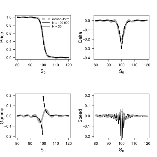
Figure 2: Price, Delta, Gamma and Speed of a digital put option with parameters $K=100$, $r=0$, $T=0.2$ and $\sigma=0.05$ as a function of $S_{0}$ and approximations using the COS method for various values of $N$. Here, $d=0\Leftrightarrow S_{0}=100.025$. For the COS method, we set $\varepsilon=10^{-5}$ and use $n=8$ moments to obtain $L=0.5$ by Equation (6).

Proof.

For $d<0$ it holds that

$$\frac{\partial^{3}P_{digital}(S_{0})}{\partial S_{0}^{3}}= \frac{-2}{\sqrt{2T}\sigma S_{0}^{3}}e^{-rT}e^{\sqrt{2}d}(1+\frac{\sqrt{2}}{\sigma\sqrt{T}})$$

$$+\frac{1}{\sqrt{2T}\sigma S_{0}^{2}}e^{-rT}e^{\sqrt{2}d}(1+\frac{\sqrt{2}}{\sigma\sqrt{T}})\sqrt{2}\frac{\partial d}{\partial S_{0}}$$

$$= \frac{-\sqrt{2}}{\sqrt{T}\sigma S_{0}^{3}}e^{-rT}e^{\sqrt{2}d}(1+\frac{\sqrt{2}}{\sigma\sqrt{T}})(1+\frac{1}{\sigma\sqrt{2T}}).$$

For $d>0$ it holds that

$$\frac{\partial^{3}P_{digital}(S_{0})}{\partial S_{0}^{3}}= \frac{-2}{\sqrt{2T}\sigma S_{0}^{3}}e^{-rT}e^{-\sqrt{2}d}(1-\frac{\sqrt{2}}{\sigma\sqrt{T}})$$

$$+\frac{1}{\sqrt{2T}\sigma S_{0}^{2}}e^{-rT}e^{-\sqrt{2}d}(1-\frac{\sqrt{2}}{\sigma\sqrt{T}})(-\sqrt{2})\frac{\partial d}{\partial S_{0}}$$

$$= \frac{-\sqrt{2}}{\sqrt{T}\sigma S_{0}^{3}}e^{-rT}e^{-\sqrt{2}d}(1-\frac{\sqrt{2}}{\sigma\sqrt{T}})(1-\frac{1}{\sigma\sqrt{2T}}).$$

∎

4 Do not apply the COS method without care

The sum appearing in Theorem 1 to approximate Speed using the COS method can always be computed because the coefficients $c_{k}^{j}$, $k=0,...,N$, $j=1,2,3$ always exist as real numbers; see Equation (4). This poses a certain mispricing risk: we show in this Section empirically that a careless application of the COS method can lead to a miscalculation of the Greeks.

As discussed in Section 3, the Gamma of a digital put option jumps at $S_{0}=S_{0}^{\ast},$ where $d(S_{0}^{\ast})=0$. The derivative of Gamma, i.e., Speed, does not exist, not even in a weak sense. One can, however, define Speed pointswise for all $S_{0}\in(0,\infty)\setminus S_{0}^{\ast}$; see Proposition 10. We show in this Section empirically that the COS method is not able to approximate the pointwise defined Speed even if we consider prices $S_{0}$ far way of the jump.

We observe in Figure 3 that the COS method does not work. In Figure 3, we consider $S_{0}\in[90,95]$. The critical point is $S_{0}^{\ast}=100.025$. The closed form of Speed exists in $[90,95]$ as a pointwise derivative. We observe that even far away from the jump point, the COS method cannot approximate the pointwise derivative of Speed at all. One reason for this strange behavior of the COS method could be the fact that the Laplace density does not satisfy Assumption A1 of Theorem 1.

5 Conclusion

In the Laplace model, we derived new formulas for the Greeks Gamma and Speed, i.e., the second and third derivatives with respect to the underlying price for European plain vanilla put and call options and digital options. The COS method is a numerical method to approximate the price and the Greeks of European options. We provided sufficient conditions for the COS method to approximate Speed. The Laplace model does not satisfy these sufficient conditions, and we showed empirically that the COS method is not able to recover the Speed of a digital put option in the Laplace model but produces nonsensical numerical results. This implies that one should apply the COS method cautiously and should check the sufficient conditions for COS method carefully.

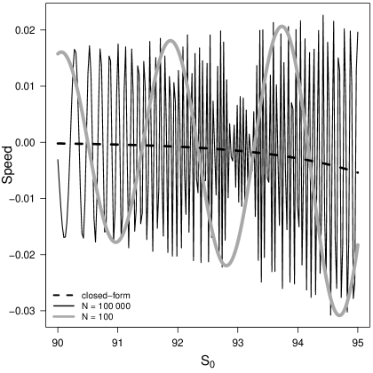
Figure 3: Speed of a digital put option with parameters as in Figure 2, i.e., $K=100$, $r=0$, $T=0.2$ and $\sigma=0.05$, as a function of $S_{0}$ and approximations using the COS method for various values of $N$. Here, $d=0\Leftrightarrow S_{0}=100.025$. For the COS method, we set $\varepsilon=10^{-5}$ and use $n=8$ moments to obtain $L=0.5$ by Equation (6). We use 200 grid points for the plot.

Declarations of Interest

The authors report no conflicts of interest. The authors alone are responsible for the content and writing of the paper.

References

• Bardgett et al. (2019) C. Bardgett, E. Gourier, and M. Leippold. Inferring volatility dynamics and risk premia from the S&P 500 and VIX markets. Journal of Financial Economics, 131(3):593–618, 2019.
• Bates (1996) D. S. Bates. Jumps and stochastic volatility: Exchange rate processes implicit in deutsche mark options. The Review of Financial Studies, 9(1):69–107, 1996.
• Fang and Oosterlee (2009a) F. Fang and C. W. Oosterlee. A novel pricing method for European options based on Fourier-cosine series expansions. SIAM Journal on Scientific Computing, 31(2):826–848, 2009a.
• Fang and Oosterlee (2009b) F. Fang and C. W. Oosterlee. Pricing early-exercise and discrete barrier options by Fourier-cosine series expansions. Numerische Mathematik, 114(1):27, 2009b.
• Fang and Oosterlee (2011) F. Fang and C. W. Oosterlee. A Fourier-based valuation method for Bermudan and barrier options under Heston’s model. SIAM Journal on Financial Mathematics, 2(1):439–463, 2011.
• Fouque et al. (2000) J.-P. Fouque, G. Papanicolaou, and K. R. Sircar. Derivatives in financial markets with stochastic volatility. Cambridge University Press, 2000.
• Garman (1992) M. Garman. Charm school. Risk, 5(7):53–56, 1992.
• Grzelak and Oosterlee (2011) L. A. Grzelak and C. W. Oosterlee. On the Heston model with stochastic interest rates. SIAM Journal on Financial Mathematics, 2(1):255–286, 2011.
• Haug (2006) E. G. Haug. The Collector: Know Your Weapon–Part 1. The Best of Wilmott, 2:23–42, 2006.
• Heston (1993) S. L. Heston. A closed-form solution for options with stochastic volatility with applications to bond and currency options. The Review of Financial Studies, 6(2):327–343, 1993.
• Junike (2023) G. Junike. How to handle the COS method for option pricing. arXiv preprint arXiv:2303.16012, 2023.
• Junike and Pankrashkin (2022) G. Junike and K. Pankrashkin. Precise option pricing by the COS method–How to choose the truncation range. Applied Mathematics and Computation, 421:126935, 2022.
• Leitao et al. (2018) Á. Leitao, C. W. Oosterlee, L. Ortiz-Gracia, and S. M. Bohte. On the data-driven COS method. Applied Mathematics and Computation, 317:68–84, 2018.
• Liu et al. (2019a) S. Liu, A. Borovykh, L. A. Grzelak, and C. W. Oosterlee. A neural network-based framework for financial model calibration. Journal of Mathematics in Industry, 9:1–28, 2019a.
• Liu et al. (2019b) S. Liu, C. W. Oosterlee, and S. M. Bohte. Pricing options and computing implied volatilities using neural networks. Risks, 7(1):16, 2019b.
• Madan (2016) D. Madan. Adapted hedging. Annals of Finance, 12(3-4):305–334, 2016.
• Madan et al. (1998) D. Madan, P. P. Carr, and E. C. Chang. The Variance Gamma process and Option Pricing. Review of Finance, 2(1):79–105, 1998.
• Madan et al. (2017) D. B. Madan, R. H. Smith, and K. Wang. Laplacian risk management. Finance Research Letters, 22:202–210, 2017.
• Oosterlee and Grzelak (2019) C. W. Oosterlee and L. A. Grzelak. Mathematical modeling and computation in finance: with exercises and Python and MATLAB computer codes. World Scientific, 2019.
• Ruijter et al. (2015) M. Ruijter, M. Versteegh, and C. W. Oosterlee. On the application of spectral filters in a fourier option pricing technique. Journal of Computational Finance, 19(1):75–106, 2015.
• Ruijter and Oosterlee (2012) M. J. Ruijter and C. W. Oosterlee. Two-dimensional Fourier cosine series expansion method for pricing financial options. SIAM Journal on Scientific Computing, 34(5):B642–B671, 2012.
• Schoutens (2003) W. Schoutens. Lévy Processes in Finance: Pricing Financial Derivatives. Wiley Online Library, 2003.
• Taleb (1997) N. N. Taleb. Dynamic hedging: managing vanilla and exotic options, volume 64. John Wiley & Sons, 1997.
• Zhang and Oosterlee (2013) B. Zhang and C. W. Oosterlee. Efficient pricing of European-style Asian options under exponential Lévy processes based on Fourier cosine expansions. SIAM Journal on Financial Mathematics, 4(1):399–426, 2013.