Dy adatom on MgO(001) substrate: DFT+U(HIA) study

Abstract

The electronic structure and magnetism of individual Dy atom adsorbed on the MgO(001) substrate is investigated using the combination of the density functional theory with the Hubbard-I approximation to the Anderson impurity model (DFT+U(HIA)). The divalent Dy²⁺ adatom in $f^{10}$ configuration is found. The calculated x-ray absorption (XAS) and magnetic circular dichroism (XMCD) spectra are compared to the experimental data. Quantum tunneling between degenerate $\ket{J=8.0,J_{z}=\pm 4.0}$ states leads to formation of $\ket{J=8.0,J_{z}=0.0}$ ground state with an in-plane orientation of the magnetic moment. It explains absence of remanent magnetization in MgO adatom on the top of Mg(001) substrate. Our studies can provide a viable route for further investigation and prediction of the rare-earth single atom magnets.

Lantanide atom adsorption on suitable surfaces is a viable pathway for creating atomic scale magnetic memories Donati2021L and quantum logic devices Thiele2014 . Dysprosium (Dy) exibits a large magnetic anisotropy and can be protected against quantum tunneling in a uniaxial crystal field Singha2021 . It has been used for molecular magnets with record-high blocking temperature goodwin2017 , and the surface adsorbed single atom magnets with the long magnetization lifetime Baltic2016 .

Recently, it was shown experimentally Donati2021 that the electronic properties of Dy adatoms on MgO thin films grown on the top of metal Ag(001) substrate change with the thickness of supporting MgO layer. X-ray absorption spectroscopy (XAS), and magnetic circular dichroism (XMCD) at 2.5 K reveal a predominance of the bulklike 4$f^{9}$ Dy for the Dy@MgO/Ag(001) with the MgO layer thickness less than 5 monolayers. By an increase of the MgO layer thickness, Dy atoms acquire the 4$f^{10}$ configuration. They display the butterfly-type magnetic hysteresis loop, indicating quantum tunneling of the magnetization (QTM).

Despite the relatively simple coordination of the atom support structure, it remains challenging to predict theoretically an influence of the substrate and adsorption geometry on the Dy 4$f$-shell charge and magnetic configurations. Theoretical calculations often require a prior knowledge of the experimental data Donati2021 . The density functional theory (DFT) is used to obtain the optimized adsorption geometry. The XAS spectra are then fitted making use of MultiX multiplet calculations Uldry2012 together with a point charge model with the positions and values of the Born charges deduced from DFT.

In this work, we present an alternative theoretical approach, based on the combination of relativistic DFT with the multiorbital impurity Hamiltonian, and apply it to investigate the electronic and magnetic character of Dy adatom at MgO(001). Our calculations suggest that the multiconfigurational aspect of the Dy 4$f$-shell together with a correct atomic limit need to be taken into account in order to reproduce the magnetic and spectroscopic properties of Dy@MgO.

The DFT+U correlated electronic structure theory in a rotationally invariant, full potential implementation shick99 ; shick01 , minimizes the total energy functional

$$E^{tot}(\rho,\hat{n})=E^{DFT}(\rho)+E^{ee}(\hat{n})-E^{dc}(\hat{n})\;,$$ (1)

where, $E^{DFT}(\rho)$ is usual density functional of the total electron and spin densities, $\rho({\bf r})$, including SOC. $E^{ee}$ is an electron-electron interaction energy and $E^{dc}$ is a “double-counting” term which accounts approximately for an electron-electron interaction energy already included in $E^{DFT}$. Both are functions of the local orbital occupation matrix $\hat{n}=n_{\gamma_{1}\gamma_{2}}$ in the subspace of the $f$ spin-orbitals $\{\phi_{\gamma}=\phi_{m\sigma}\}$.

Minimization of the DFT+U total energy functional Eq. 1 leads to the solution of the generalized Kohn–Sham-Dirac equations,

$$\bigl{[}-\nabla^{2}+{V}_{\rm DFT}(\mathbf{r})+(V_{U}-V_{dc})+\xi({\bf l}\cdot{\bf s})\bigr{]}\Phi_{\bf k}({\bf r})=\epsilon_{\bf k}\Phi_{\bf k}({\bf r}),$$ (2)

where, ${V}_{U}$ is an effective DFT+U potential, and $V_{dc}$ is the spherically-symmetric DFT+U double-counting term AZA1991 ; solovyev1994 The self-consistent solition of in Eq.(2) generates not only the ground state energy and charge/spin densities, but also effective one-electron states and energies. The basic difference of DFT+U calculations from DFT is its explicit dependence on the on-site spin- and orbitally resolved $n_{\gamma_{1}\gamma_{2}}$ occupation matrices .

The fundamental limitation of DFT+U calculations is that they rely on a single Slater determinant approximation for the $f$-manifold. However, as pointed out in Ref. shick2001 ; Dorado2013 , it makes the DFT+U results extremely sensitive to the initial conditions, which leads to numerious metastable solutions.

In order to avoid convergence to a metastable state, various strategies have been proposed. The occupation matrix control (OMC) has recently been exploited by Krack Krack2015 for the two $f$-electrons, however the identified ground state does not agree with earlier DFT+U results of Dorado et al. Dorado2010 . Alternatively, the so-called $U$-ramping method relies on a gradual increase of the Coulomb-$U$ parameter of DFT+U. While this approach has had some success, it has been shown to give higher energies than the OMC method Meredig2010 .

Recently, we proposed the extention of DFT+U SFP2021 making use of a combination of DFT with the exact diagonalization of the Anderson impurity model Hewson . The complete seven-orbital 4$f$ shell model includes the full spherically symmetric Coulomb interaction, the spin-orbit coupling, and the crystal field. The corresponding Hamiltonian can be written as,

$$\hat{H}_{\text{imp}}= \sum_{m\sigma}\epsilon_{f}f^{\dagger}_{m\sigma}f_{m\sigma}$$ (3)

$$+\sum_{mm^{\prime}\sigma\sigma^{\prime}}\bigl{[}\xi{\bf l}\cdot{\bf s}+\hat{\Delta}_{\rm CF}+\frac{\Delta_{\rm EX}}{2}\hat{\sigma}_{z}\bigr{]}_{mm^{\prime}}^{\sigma\;\;\sigma^{\prime}}f_{m\sigma}^{\dagger}f_{m^{\prime}\sigma^{\prime}}$$

$$+\frac{1}{2}\sum_{\begin{subarray}{c}mm^{\prime}m^{\prime\prime}\\ m^{\prime\prime\prime}\sigma\sigma^{\prime}\end{subarray}}U_{mm^{\prime}m^{\prime\prime}m^{\prime\prime\prime}}f^{\dagger}_{m\sigma}f^{\dagger}_{m^{\prime}\sigma^{\prime}}f_{m^{\prime\prime\prime}\sigma^{\prime}}f_{m^{\prime\prime}\sigma},$$

where $f^{\dagger}_{m\sigma}$ creates a 4$f$ electron. The $\xi$ parameter specifies the SOC strength, and is taken from DFT calculations in a standard way MPK1980 , making use of the radial solutions of the Kohn- Sham-Dirac scalar-relativistic equations (2), and the radial derivative of spherically- symmetric part of the DFT potential. $\Delta_{\rm CF}$ is the crystal-field potential, and $\Delta_{\rm EX}$ is the exchange field strength. The parameter $\epsilon_{f}$ ($=-\mu$, the chemical potential) defines the number of $f$-electrons. The last term describes the Coulomb interaction in the $f$-shell. Actual choice of these parameters will be discussed later.

This model assumes the weakness of the hybridization between the localized $f$-electrons and the itinerant $s$, $p$, and $d$-states described in DFT. Thus, the quantum impurity Anderson model Hewson is reduced to the atomic limit, and corresponds to the Hubbard-I approximation (HIA).

The Lanczos method Kolorenc2012 is employed to find the lowest-lying eigenstates of the many-body Hamiltonian $H_{\text{imp}}$ and to calculate the selfenergy matrix $[\Sigma(z)]_{\gamma,\gamma^{\prime}}$ in the subspace of the $f$ spin-orbitals $\{\phi_{\gamma}=\phi_{m\sigma}\}$ at low temperature ($k_{\rm B}T=\beta^{-1}=2$ meV). Once the selfenergy is found, the local Green’s function $G(z)$ for the electrons in the 4$f$ manifold reads,

$$G(z)=\Big{(}[{G(z)}_{\rm DFT}]^{-1}+\Delta\epsilon-\Sigma(z)\Big{)}^{-1}\,,$$ (4)

where ${G}_{\rm DFT}(z)$ is the “non-interacting” DFT Green’s function, and $\Delta\epsilon$ is chosen so as to ensure that $n_{f}\;=\;-\pi^{-1}{\rm Im}\;{\rm Tr}\int_{-\infty}^{E_{\rm{F}}}{\rm d}z[G(z)]$ is equal to the number of 4f electrons derived from Eq. (2). Then, with the aid of the local Green’s function $G(z)$, we evaluate the occupation matrix $n_{\gamma_{1}\gamma_{2}}=-\pi^{-1}\mathop{\rm Im}\int_{-\infty}^{E_{\rm{F}}}{\rm d}z\,[G(z)]_{\gamma_{1}\gamma_{2}}$.

This matrix $n_{\gamma_{1}\gamma_{2}}$ is used to construct an effective DFT+U potential ${V}_{U}$ in Eq.(2). Note that the DFT potential ${V}_{\rm DFT}$ in Eq.(2) acting on the $f$-states is corrected to exclude the non-spherical double-counting with $V_{U}$ Kristanovski2018 . The equations Eq.(2) are iteratively solved until self-consistency over the charge density is reached. The new DFT Green’s function ${G}_{\rm DFT}$ and the new value of the 5$f$-shell occupation are obtained from the solutions of Eq. (2). The next iteration is started by solving Eq. (3) with the updated value of $\epsilon_{f}=-\mu$ in Eq. (3), which is determined by the condition $\mu=V_{dc}$ SFP2021 .

The loop procedure is repeated until the convergence of the 4$f$-manifold occupation $n_{f}$ is better than 0.02. After the self-consistent solution of DFT+U(HIA) is obtained, the mean-field total energy $E_{Tot}=E_{\rm DFT}+\Delta E^{ee}$ is calculated as a sum of DFT total energy $E_{\rm DFT}$, and the energy correction $\Delta E^{ee}\;=\;E^{ee}\;-\;E_{dc}$. Importantly, this solution is unique as it stems from the many-body ground state of  Eq. (3) with the exact atomic limit.

We make use of the $2\times 2\times 1$ lateral supercell ($a=4.21$ Å) of 3 ML of MgO to which the rare-earth Dy adatom is added on the oxyden site. In order to obtain the supercell geometry, we performed the standard DFT (with the exchange-correlation functional of Perdew, Burke and Ernzerhof PBE ) Vienna ab initio simulation package (VASP VASP ) calculations together with the projector augmented-wave method (PAW PBE ). Moreover, assuming that localised 4$f$ electrons have rather small impact on the geometry, we used the rare-earth Lu adatom instead of Dy, and treated 14 closed 4$f$-shell electrons of Lu as valence. The system was relaxed until the forces on the Lu adatom and on top-most 2 ML of MgO are 0.001 eV/Å. The calculated 2.1 Å Lu-O bond length to the underneath oxygen is in a good quantitative agreement with the DFT+U results of Ref. Donati2021 for Dy-O bond length. Calculated adsorption geometry is shown in the Fig. 1.

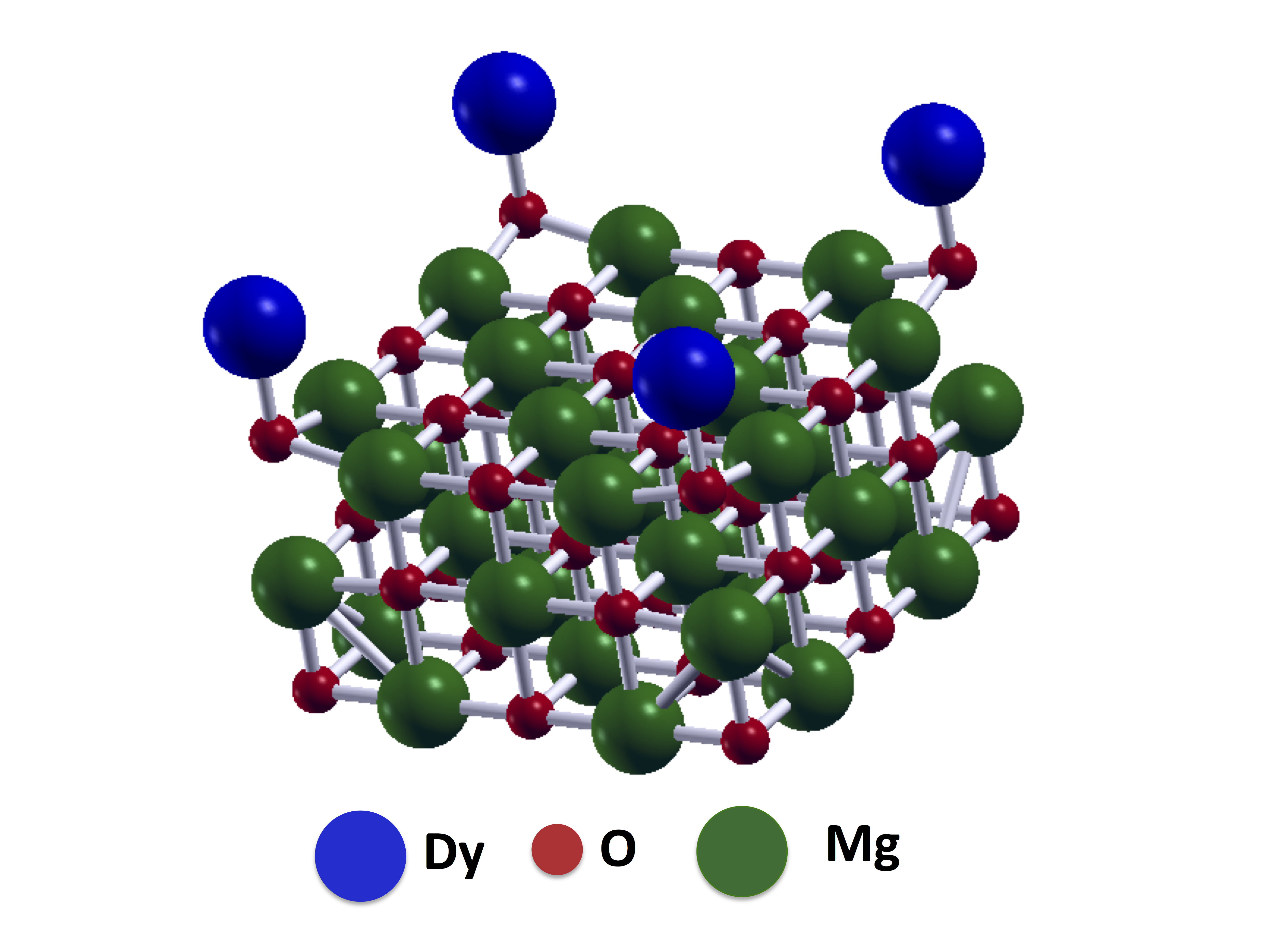
Figure 1: Supercell model for rare-earth impurity on MgO(001). Dy atoms are shown in blue, O atoms are in red, and Mg atoms in green.

The structural information obtained from the VASP simulations was used as an input for further DFT+U(HIA) electronic structure calculations that employ the relativistic version of the full-potential linearized augmented plane-wave method (FP-LAPW) FLAPW . In the FP-LAPW the SOC is included in a self-consistent second-variational procedure shick1997 . This two-step approach synergetically combines the speed and ef- ficiency of the highly optimized VASP package with the state-of-the-art accuracy of the FP-LAPW method

The Slater integrals $F_{0}=7.00$ eV, and $F_{2}=9.77$ eV, $F_{4}=6.53$ eV, and $F_{6}=$4.83 eV were chosen to parametrize the Coulomb interaction term in Eq. (3), and to construct the DFT+U potential ${V}_{U}$ in the Eq. (2). They corresponds to the values for Coulomb $U=7.00$ eV and exchange $J=0.82$ eV. The above choice of the Slater integrals is justified shick2020 by agreement between the density of states (DOS) calculated with DFT+U(HIA) and the experimental valence band photoemission for the bulk Dy.

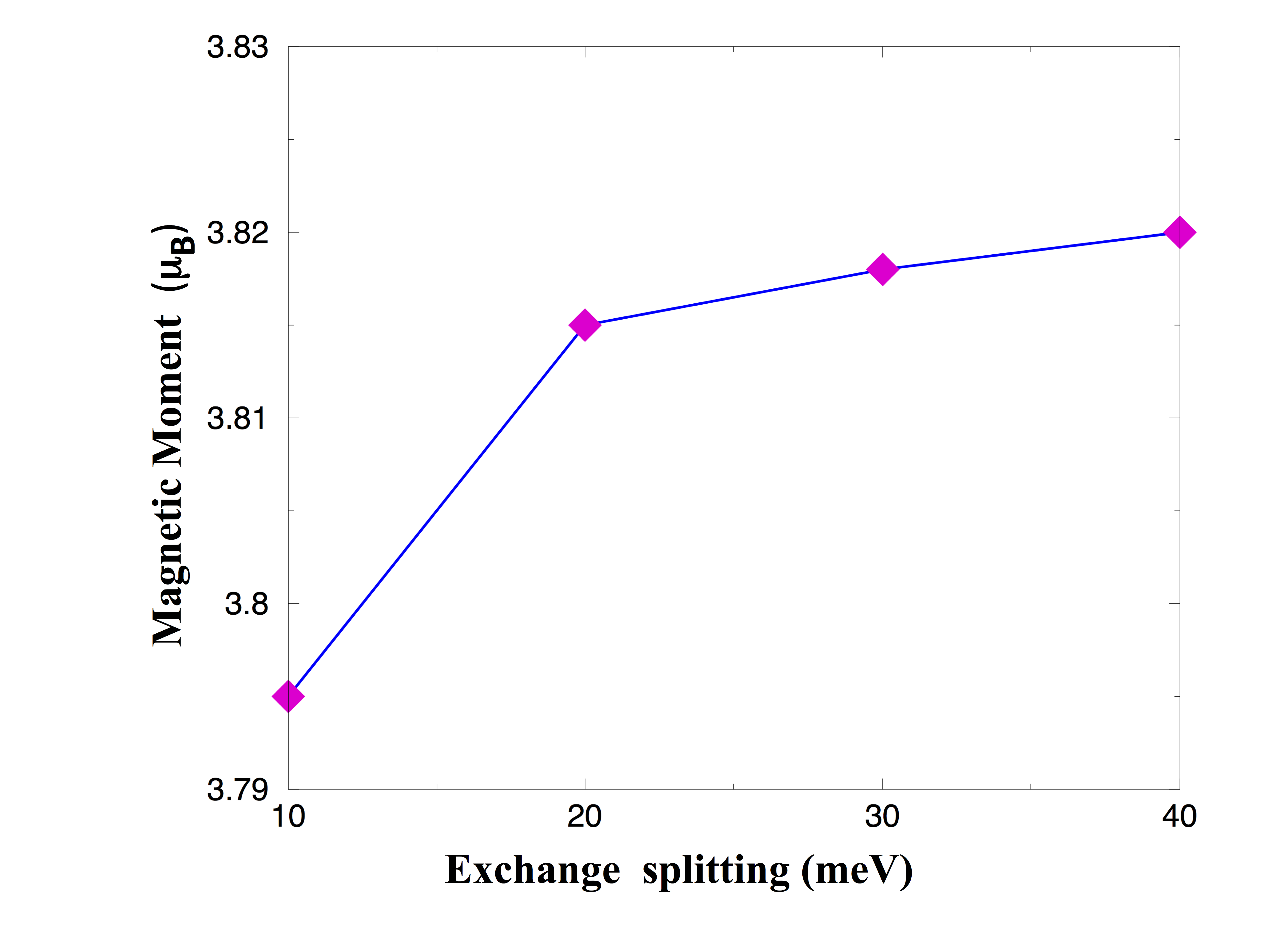
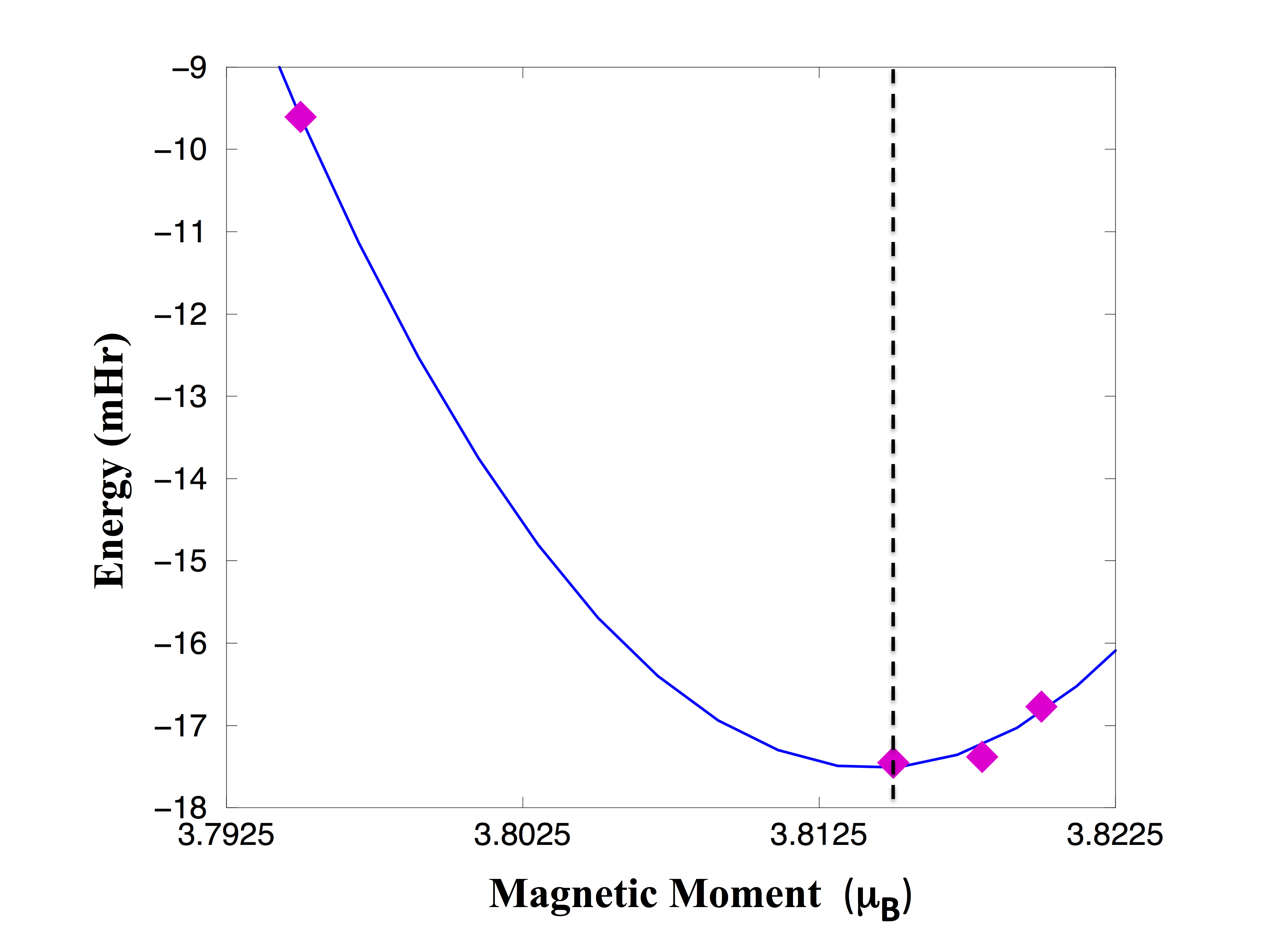
Figure 2: The total spin magnetic moment per unit cell vs the exchange splitting $\Delta_{EX}$ dependence (A); the total energy as a function the magnetic moment dependence, $E^{tot}(M)=const+\alpha M^{2}-\beta M^{4}$. The total energy minimum position is marked by dashed line.

The exchange splitting $\Delta_{\rm EX}$ in the Eq. (3) corresponds to the interorbital exchange energy between the localized 4$f$ and itinerant $s$ and $d$ shells Peters2014 ; piveta2020 . The $\Delta_{\rm EX}$ can be estimated as

$$\Delta_{\rm EX}=2J_{fs}S_{6s}+2J_{fd}S_{5d}\;,$$

where $J_{fs}$ and $J_{fd}$ are the interorbital exchange constants piveta2020 . The spin-polarized DFT calculations with the magnetization directed along the $z$-axis yield $\Delta_{\rm EX}\approx$ 10 meV, which can be taken as a lower bound value for the interorbital exchange energy  Peters2014 .

We performed the DFT+U(HIA) calculations treating $\Delta_{\rm EX}$ as a parameter in the Eq. (3). In these spin-polarized calculations we applied the DFT non-spin-polarized exchange-correlation potential to the $f$-states in the Eq. (2), in order to exclude the contribution of $f$-intraorbital exchange field into the double-counting $V_{dc}$. The spin-polarized functional is used for all other states.

We solve self-consistently the Eq. (2), and obtain dependence of the total spin magnetic moment per unit cell $M(\Delta_{\rm EX})$ (see Fig. 2A) and the total energy $E^{tot}(\Delta_{\rm EX})$ Eq. (1) on the magnitude of the $\Delta_{\rm EX}$. Note that the upper bound limit of $\Delta_{\rm EX}\approx$ 40 meV is set by reaching the saturation of the magnetic moment.

The total energy vs the magnetic moment dependence $E^{tot}(M)$ is shown in Fig. 2B. Using the Landau expansion LL1980 of the magnetic energy,

$$E^{tot}(M)=const+\alpha M^{2}-\beta M^{4}$$

we obtain the magnetic moment $M=\sqrt{\alpha\over{2\beta}}$ which corresponds to the minimum of the $E^{tot}$. The corresponding value of $\Delta_{\rm EX}\approx 20$ meV yields the value of the interorbital exchange energy in the Eq. (3).

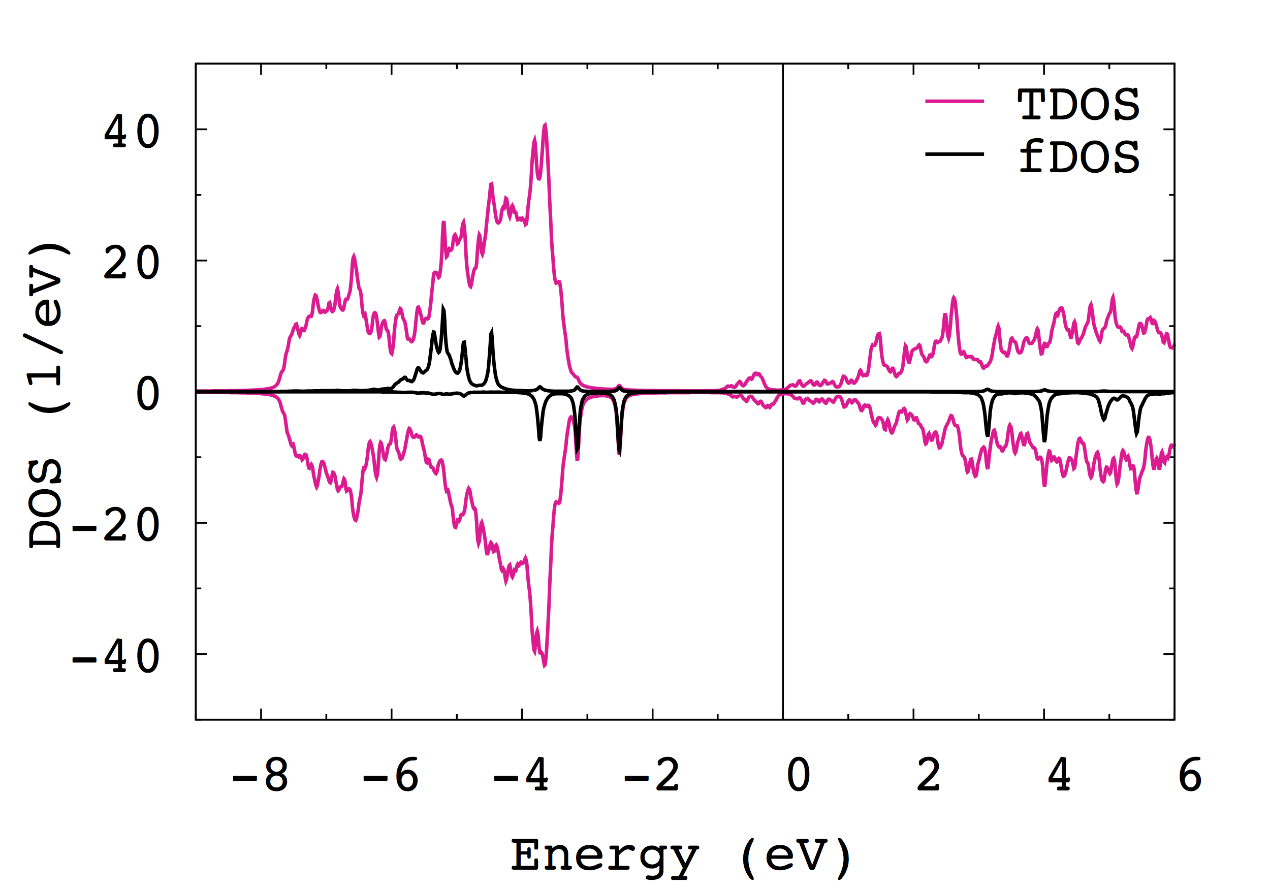
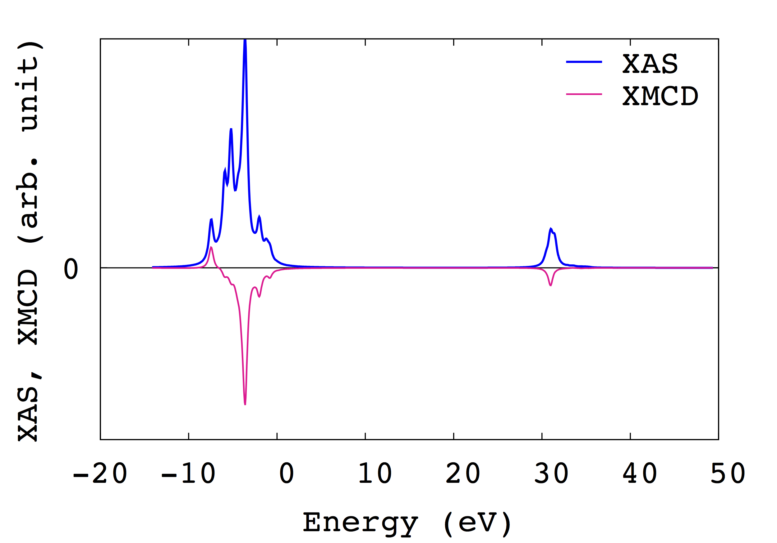
Figure 3: The spin-resolved total (TDOS) and the $f$-projected ($f$DOS) DOS (A); the M-edge XAS and XMCD spectra (normal incidence) (B) for Dy@MgO(001)

Table 1: The $f$-electron occupation $n_{f}$ , spin $\langle M_{S}\rangle$, orbital $\langle M_{L}\rangle$, $\langle M_{S}\rangle$ plus magnetic dipole $\langle M_{D}\rangle$ moments (in $\mu_{B}$), and the ratio $R_{LS}={{\langle M_{L}\rangle}\over{\langle M_{S}\rangle+\langle M_{D}\rangle}}$ for the Dy adatom on MgO(001). The nonzero Stevens parameters $B_{k}^{q}$ (in $\mu eV$).

	$n_{f}$	$\langle M_{S}\rangle$	$\langle M_{L}\rangle$	$\langle M_{S}\rangle$+$\langle M_{D}\rangle$	$R_{LS}$
Dy@MgO	9.91	3.65	5.92	4.64	1.28

CEF	$B_{2}^{0}$	$B_{4}^{0}$	$B_{6}^{0}$	$B_{4}^{4}$	$B_{6}^{4}$
	-20.55	0.23	-0.02	1.81	0.04

The calculated ground state $f$-electron occupation $n_{f}={\rm Tr}[\hat{n}]$, magnetic spin $\langle M_{S}\rangle=-2\langle S_{z}\rangle\mu_{B}/\hbar=-{\rm Tr}[\hat{\sigma}_{z}\hat{n}]\mu_{B}/\hbar$, orbital $\langle M_{L}\rangle=-\langle L_{z}\rangle\mu_{B}/\hbar$, dipole $\langle M_{D}\rangle=-6\langle T_{z}\rangle\mu_{B}/\hbar$ moments, and $R_{LS}={{\langle M_{L}\rangle}\over{\langle M_{S}\rangle+\langle M_{D}\rangle}}$ value, the ratio of the orbital to the effective spin moment, are shown in Table 1. The itinerant part of the magnetization of 0.10 $\mu_{B}$ includes the Dy adatom 6$s$-states $m_{6s}$ = 0.02 $\mu_{B}$, and 5$d$-states $m_{5d}$ = 0.02 $\mu_{B}$ magnetic moments. Note that the calculation of these moments is associated with some uncertainty, and depends on the choice of the Dy adatom muffin-tin radius.

The total (TDOS) and $f$-projected ($f$DOS) DOS calculated from the solutions of the Eq.(2) are shown in Fig. 3 (A). The MgO band gap is at $\approx$ 3-to-1 eV below the Fermi level. The sharp 4$f$-spin-$\downarrow$ peaks are located at the top of MgO valence band gap. The smooth TDOS peak $\approx$ 1 eV below the Fermi level has a capacity of 2 electrons which are transfered from the Dy adatom to the MgO substrate.

The $f$-electron occupation $n_{f}=9.91$ is consistent with the $f^{10}$ configuration obtained from Eq. (3), and defines the Dy adatom valence as Dy²⁺. We used the Eq. (3), with the self-consistently determined parameters as an input for the Quanty code quanty to estimate the M-edge XAS and XMCD spectra (see for details Supplemental material). The computed spectra (Fig. 3B) are in a reasonable agreement with available experimental data Donati2021 .

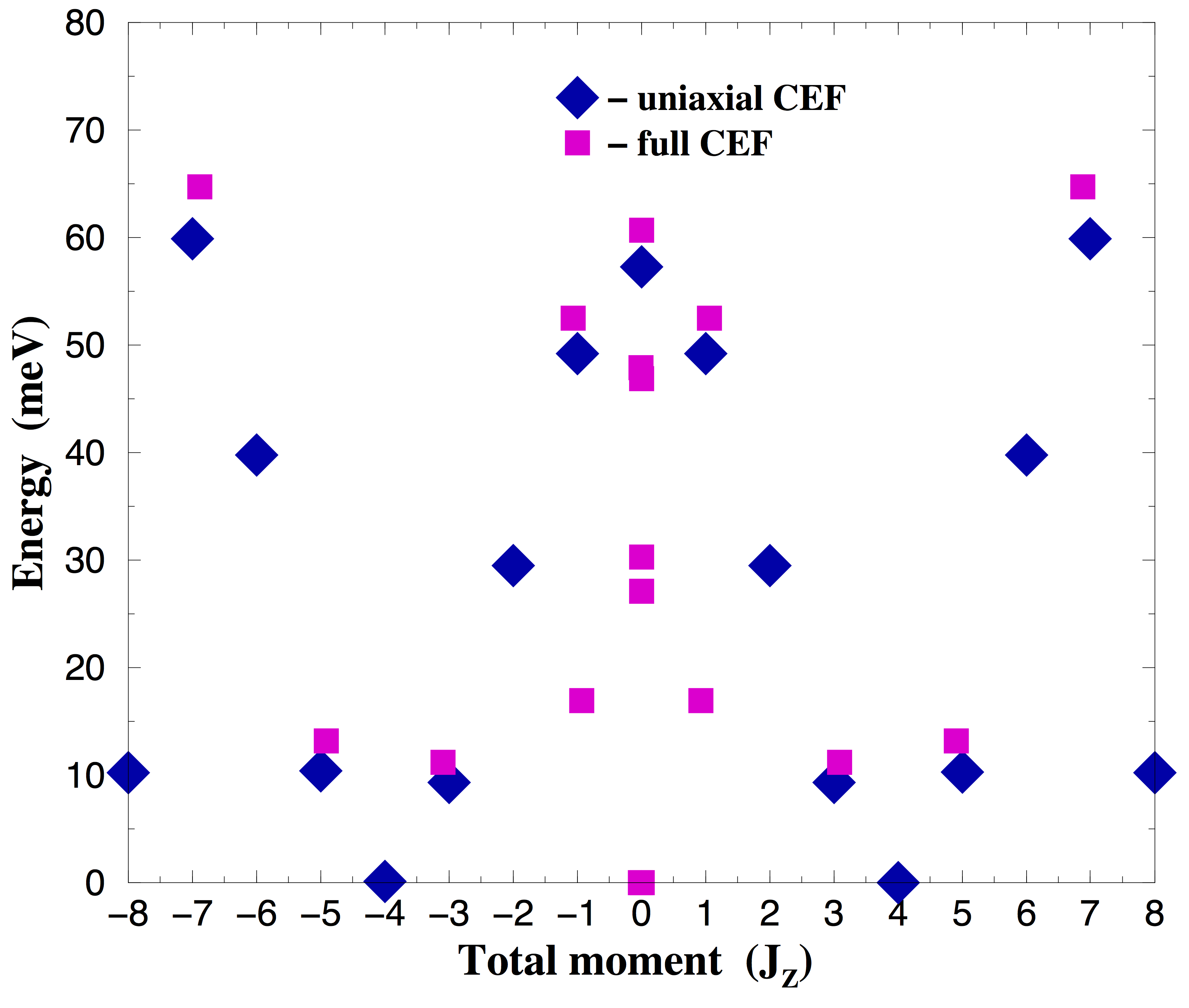
Figure 4: Scheme of quantum many-body levels of the lowest $J=8.0$ multiplet obtained from the solutions of Eq.  (3) ($\Delta_{\rm ex}=0$) with the $\Delta_{\rm CF}$ parameters taken from spin-polarized calculations (squares); energy diagram of the CF Hamiltonian with the uniaxial CEF parameters only (diamonds).

The scheme of quantum many-body levels of the lowest $J=8.0$ multiplet obtained from the solutions of Eq. (3) is shown in Fig. 4. Without an external magnetic field, the lowest energy state of Eq. (3) is a singlet $\ket{J=8.0,J_{z}=0.0}$ state. There is another $\ket{J=8.0,J_{z}=0.0}$ singlet with the energy of 0.06 meV above the ground state. Leaving the only uniaxial (diagonal) contributions to the $\Delta_{\rm CF}$ yields the $\ket{J=8.0,J_{z}=\pm 4.0}$ ground state (cf. Fig. 4).

The $\Delta_{\rm CF}$ matrix calculated in the DFT+U(HIA) is used to build the CF hamiltonian shick2019 for the Dy@MgO(001),

$$\hat{H}_{CF}=\sum_{kq}B_{k}^{q}\hat{O}_{k}^{q}\;,$$ (5)

where $\hat{O}_{k}^{q}$ are the Stevens operator equivalents, and $B_{k}^{q}$, the Stevens crystal field parameters (in standard notations) for given $k$ and $q$. The five evaluated non-zero Stevens parameters, $B_{2}^{0}$, $B_{4}^{0}$, $B_{6}^{0}$, $B_{4}^{4}$, and $B_{6}^{4}$ are shown in Table. 1. The energy diagrams of the CF hamiltonian (5) are shown in Fig. 5 (see Supplemental material. Both diagrams, with the full set of the CF parameters, and with the first three uniaxial CF parameters are shown). It is seen that the CF solutions approximate reasonably well the many-body solutions of the Eq. (3) shown in Fig 4.

The first three parameters $B_{2}^{0}$, $B_{4}^{0}$, $B_{6}^{0}$ yield the uniaxial splitting between different $J_{z}$ eigenstates in Eq. (5) with the $\ket{J=8.0,J_{z}=\pm 4.0}$ ground state, and correspond to diagonal contributions to the $\Delta_{\rm CF}$. The energy difference between the lowest and highest $J_{z}$ levels, the so-called zero field splitting (ZFS) of 65 meV is found, which is related to the uniaxial magnetic anisotropy baltic2018 . The transverse $B_{4}^{4}O_{4}^{4}$ term in the CF hamiltonian connects the $\ket{J=8.0,J_{z}=\pm 4.0}$ states so that the quantum tunneling of the magnetization (QTM) occurs between these two states, and the resulting $\ket{J=8.0,J_{z}=0}$ ground state corresponds to the “in-plane” magnetic moment orientation. It explains an absence of the remanent magnetization in Dy@MgO(001) observed experimentally Donati2021 .

To conclude, the electronic structure and magnetism of individual Dy atom adsorbed on the MgO(001) substrate is investigated using the combination of the density functional theory with the Hubbard-I approximation to the Anderson impurity model. The divalent Dy²⁺ adatom is found with a singlet $\ket{J=8.0,J_{z}=0.0}$ ground state. The calculated XAS and XMCD spectra are in reasonable agreement with available experimental data. No remanent magnetization is found due to QTM, in agreement with experimentally observed butterfly-type magnetic hysteresis loop.

We acknowledge stimulating discussions with J. Kolorenc and A. Yu. Denisov. Financial support was provided by Operational Programme Research, Development and Education financed by European Structural and Investment Funds and the Czech Ministry of Education, Youth and Sports (Project No. SOLID21 - CZ.02.1.01/0.0/0.0/16_-019/0000760), by the Czech Science Foundation (GACR) Grant No. 22-22322S, and from the Israeli Ministry of Aliyah and Integration Grant Ref.:140636.

Appendix A Supplemental Material

A.1 Computational details

In the DFT+U(HIA) FP-LAPW calculations, 49 special k-points in the two-dimensional Brillouin zone were used, with Gaussian smearing for k-points weighting. The “muffin-tin” radii of $R_{MT}\;=\;2.70\;a.u.$ for Dy, $R_{MT}=1.20$ a.u. for O, $R_{MT}=2.00$ a.u. for Mg were used. The LAPW basis cut-off is defined by the condition $R^{Dy}_{MT}\times K_{max}\;=\;8.10$ (where $K_{max}$ is the cut-off for LAPW basis set).

The CF matrix $\Delta_{\rm CF}$ in Eq.(3) is obtained by projecting the self-consistent solutions of Eq.(2) into the $\{\phi_{\gamma}\}$ local $f$-shell basis, giving the “local Hamiltonian”

$$[H_{loc}]_{\gamma\gamma^{\prime}} = \int_{\epsilon_{b}}^{\epsilon_{t}}{\rm d}\epsilon\,\epsilon[N(\epsilon)]_{\gamma\gamma^{\prime}}$$ (6)

$$\approx \epsilon_{0}\delta_{\gamma\gamma^{\prime}}+[\xi{\bf l}\cdot{\bf s}+\Delta_{\rm CF}]_{\gamma\gamma^{\prime}}+[{V_{U}}]_{\gamma\gamma^{\prime}}\,,$$

where $[N(\epsilon)]_{\gamma_{1}\gamma_{2}}$ is the $f$-projected density of states (fDOS) matrix

$$[N(\epsilon)]_{\gamma_{1}\gamma_{2}}\;=\;-\pi^{-1}{\rm Im}{[G(z)_{\rm DFT+U}]}_{\gamma_{1}\gamma_{2}}\;,$$

$\epsilon_{b}$ is the bottom of the valence band, $\epsilon_{t}$ is the upper cut-off, which is naturally defined by the condition $\int_{\epsilon_{b}}^{\epsilon_{t}}{\rm d}\epsilon\,{\rm Tr}{[N(\epsilon)]}\;=14$, and $\epsilon_{0}$ is the mean position of the non-interacting $5f$ level. The matrix $\Delta_{\rm CF}$ is then obtained by removing the interacting DFT+$U$ potential $[{V_{U}}]_{\gamma\gamma^{\prime}}$ and SOC $[\xi{\bf l}\cdot{\bf s}]_{\gamma\gamma^{\prime}}$ from $H_{loc}$ Eq.( 6).

A.2 Calculation of XAS and XMCD spectra

We used the ionic hamiltonian, Eq. (3), with the self-consistently determined $\Delta_{CF}$ parameters as an input for the Quanty code quanty to estimate the M-edge XAS and XMCD spectra. In these calculations, the exchange field $\Delta_{\rm EX}$ is replaced with the external magnetic field $B_{z}=6.8$ T typical in the experimental XMCD measurements singha2017 . The 3d–4f Coulomb interaction is parametrized with Slater integrals computed with the Cowan’s Hartree–Fock code cowan and then reduced to 80% to approximately account for screening (Table 2). The 3d spin-orbit coupling $\xi_{3d}=14.4$ eV is taken from the same Hartree–Fock calculations.

Table 2: Slater integrals defining the 3d–4f Coulomb interaction as computed with the Cowan’s code cowan for the XAS final state 3d⁹4f¹¹. The Hartree–Fock values are reduced to 80% to account for screening. All values are shown in eV.

	$F_{2}$	$F_{4}$	$G_{1}$	$G_{3}$	$G_{5}$
3d94f11	7.36	3.44	5.28	3.10	2.14

A.3 Crystal-field model parameters

The energy diagrams of the CF Hamiltonian (5) with the CF parameters from Table I of the main text. are shown in in Fig. 5. Both diagrams, with the full set of five Stevens parameters, and with the first three uniaxial CF parameters are shown. It is seen that the CF solutions approximate reasonably well the many-body solutions of the Eq. (3) shown in Fig. 4 of the main text. The first three CF parameters $B_{2}^{0}$, $B_{4}^{0}$, $B_{6}^{0}$ yield the uniaxial splitting of different $J_{z}$ eigenstates in Eq. (5), and the $\ket{J=8.0,J_{z}=\pm 4.0}$ ground state. The energy difference between the lowest and highest $J_{z}$ levels (ZFS) of 65 meV is found. Once the nonzero transverse CF parameters $B_{4}^{4}$, and $B_{6}^{4}$ are included in Eq.(5), the ground state becomes a singlet $\ket{J=8.0,J_{z}=0}$ with another singlet $\ket{J=8.0,J_{z}=0}$ with the energy of 0.5 meV above the ground state.

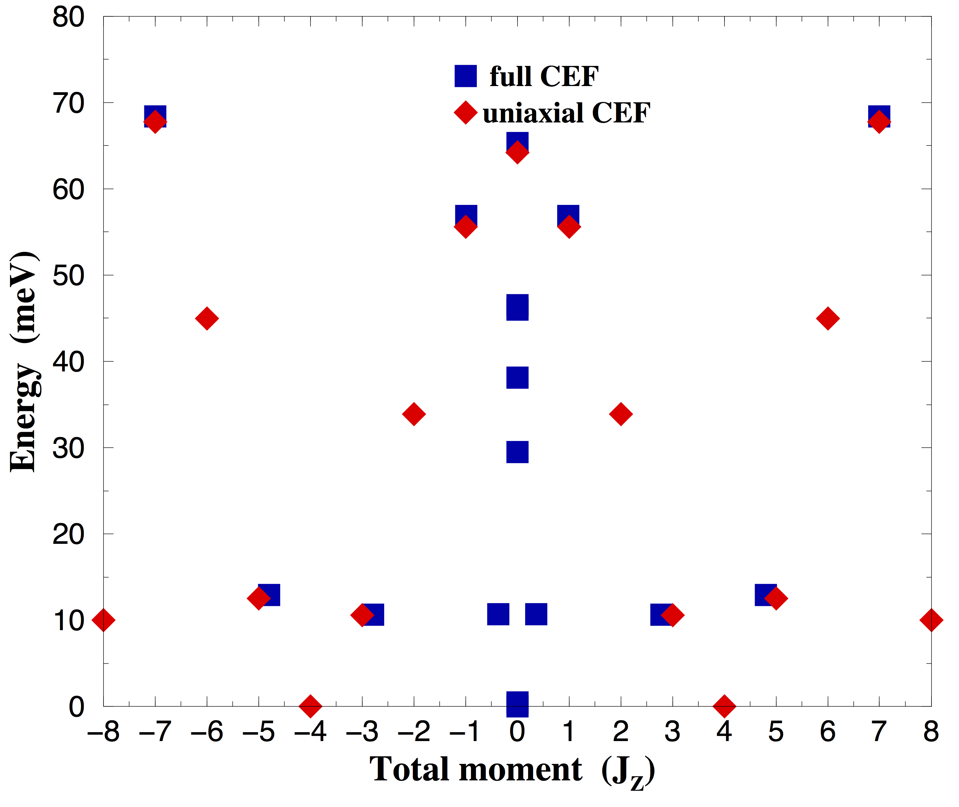
Figure 5: The energy diagram of the CF Hamiltonian with the CF parameters from Table I. (squares), and the uniaxial CEF only (diamonds).

References

- (1) F. Donati, A. J. Heirich, Appl. Phys. Lett. 119, 160503 (2021).
- (2) S. Thiele et al., Science 344, 1135 (2014).
- (3) A. Singha et al., Nature Communications 12, 4179 (2021).
- (4) C.A.P. Goodwin, F. Ortu, D. Reta, N.F. Chilton, D. P. Mills, Nature 548, 439 (2017).
- (5) R. Baltic et al., Nano Lett. 16, 7610 (2016).
- (6) F. Donati et al., Nano Lett. 21, 8266 (2021).
- (7) A. Uldry, F. Vernay, B. Delley, Phys. Rev. B 85, 125133 (2012).
- (8) A. B. Shick, A. I. Liechtenstein, W. E. Pickett, Phys. Rev. B 60, 10763 (1999).
- (9) A. B. Shick, W. E. Pickett, Phys. Rev. Lett. 86, 300 (2001).
- (10) V. I. Anisimov, J. Zaanen, O. K. Andersen, Phys. Rev. B 44, 943 (1991).
- (11) I. V. Solovyev, P. H. Dederichs, V. I. Anisimov, Phys. Rev. B 50, 16861 (1994).
- (12) O. Kristanovski, A. B. Shick, F. Lechtermann, A. I. Lichtenstein, Phys. Rev. B 97, 201116 (2018).
- (13) A. B. Shick, W. E. Pickett, A. I. Liechtenstein, J. Electr. Spectr. Phenom. 114, 753 (2001).
- (14) B. Dorado, M. Freyss, B. Amadon et al., J. Phys.: Condens. Matt. 25, 333201 (2013).
- (15) M. Krack, Phys. Scr. 90, 094014 (2015).
- (16) B. Dorado, G. Jomard, M. Freyss, M. Bertolus, Phys. Rev. B 82, 035114 (2010).
- (17) B. Meredig et al., Phys. Rev. B 82, 195128 (2010).
- (18) A. B. Shick, S.-i. Fujimori, W. E. Pickett, Phys. Rev. B 103, 125136 (2021).
- (19) A. Hewson, The Kondo Problem to Heavy Fermions, Cambridge University Press, 1993.
- (20) A. MacDonald, W. Pickett and D. Koelling , J. Phys. C: Solid State Phys. 13, 2675 (1980).
- (21) J. Kolorenc, A. I. Poteryaev, A. I. Lichtenstein, Phys. Rev. B 85, 235136 (2012).
- (22) J. P. Perdew, K. Burke, and M. Ernzerhof, Phys. Rev. Lett. 77, 3865 (1996).
- (23) G. Kresse and J. Furthmuller, Phys. Rev. B 54, 11169 (1996).
- (24) P. E. Blochl, Phys. Rev. B 50, 17953 (1994).
- (25) E. Wimmer, H. Krakauer, M. Weinert, and A. J. Freeman, Phys. Rev. B. 24, 864 (1981).
- (26) A. B. Shick, D. L. Novikov, and A. J. Freeman, Phys. Rev. B 56, R14259 (1997)
- (27) A. B. Shick, J. Kolorenc, A. Y. Denisov, and D. S. Shapiro, Phys. Rev. B 102, 064402 (2020).
- (28) L. Peters et al., Phys. Rev. B 89, 205109 (2014).
- (29) M. Piveta et al., Phys. Rev. X 10, 031054 (2020).
- (30) L. D. Landau, and E. M. Lifshits, Statistical Physics, 3rd Edition Part I, Elsevier, 1980.
- (31) M. W. Haverkort, M. Zwierzcki, O. K. Andersen, Phys. Rev. B 85, 165113 (2012).
- (32) A. B. Shick, A. Yu. Denisov, J. Magn. Magn. Mater. 475, 211 (2018).
- (33) R. Baltic et al., Phys. Rev. B 98, 024412 (2018).
- (34) A. Singha, R. Baltic, F. Donati et al., Phys. Rev. B 96, 224418 (2017).
- (35) R. D. Cowan, The theory of atomic structure and spectra, University of California Press, Berkeley, 1981.