Frigate: Frugal Spatio-temporal Forecasting on Road Networks

Abstract.

Modelling spatio-temporal processes on road networks is a task of growing importance. While significant progress has been made on developing spatio-temporal graph neural networks (Gnns), existing works are built upon three assumptions that are not practical on real-world road networks. First, they assume sensing on every node of a road network. In reality, due to budget-constraints or sensor failures, all locations (nodes) may not be equipped with sensors. Second, they assume that sensing history is available at all installed sensors. This is unrealistic as well due to sensor failures, loss of packets during communication, etc. Finally, there is an assumption of static road networks. Connectivity within networks change due to road closures, constructions of new roads, etc. In this work, we develop Frigate to address all these shortcomings. Frigate is powered by a spatio-temporal Gnn that integrates positional, topological, and temporal information into rich inductive node representations. The joint fusion of this diverse information is made feasible through a novel combination of gated Lipschitz embeddings with Lstms. We prove that the proposed Gnn architecture is provably more expressive than message-passing Gnns used in state-of-the-art algorithms. The higher expressivity of Frigate naturally translates to superior empirical performance conducted on real-world network-constrained traffic data. In addition, Frigate is robust to frugal sensor deployment, changes in road network connectivity, and temporal irregularity in sensing.

1. Introduction and Related Work

Figure 1. Snapshots of selected roads from Beijing and Chengdu displaying the tidal variation of traffic

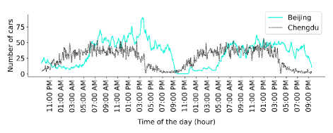
A road network can be modeled as a graph where nodes indicate important intersections in a region and edges correspond to streets connecting two intersections (Pande et al., 2017; Yawalkar and Ranu, 2019; Mitra et al., 2017, 2015; Joshi et al., 2021; Medya et al., 2018). Modeling the evolution of spatio-temporal events on road networks has witnessed significant interest in the recent past (Li et al., 2018; Yu et al., 2018; Fang et al., 2021; Yang et al., 2021; Wu et al., 2019). Specifically, each node (or edge) participates in a time-series. This time-series is a function of not only the time of the day, but also the events unfolding in other nodes of the network. The objective of the forecasting task is to model the time-series evolution in each node and predict the values in the immediate future, for e.g., the next one hour. As examples, in Fig. 1, we present the number of cars passing through two randomly selected intersections in the cities of Beijing and Chengdu. As can be seen, there is significant variation in traffic through out the day. Furthermore, the time-series vary across nodes making the forecasting problem non-trivial.

One may learn an auto-regressive model independently at each node to fit the time-series data. This strategy, however, is limited by two critical factors. First, this ignores the connectivity-induced time-series dependency among nodes. For example, if one particular intersection (node) is observing traffic congestion, it is likely for neighboring nodes connected through an outgoing edge to be affected as well. Second, the number of parameters grows linearly with the number of nodes in the graph, making it non-scalable.

1.1. Existing work

To address these specific needs of modeling network-dependent spatio-temporal processes, several algorithms merging models for structural data such as Gnns (Yu et al., 2018; Lan et al., 2022; Li and Zhu, 2021) or Convolutional neural networks (Yang et al., 2021) along with auto-regressive architectures have been developed. The proposed work is motivated based on some assumptions made by existing algorithms that are not realistic for real-world road networks. Table 1 summarizes these.

• Ability to extrapolate from partial sensing: Several of the existing algorithms assume that a sensor is placed in each node of the road network (Bai et al., 2020; Zheng et al., 2020; Wu et al., 2019; Lan et al., 2022; Song et al., 2020; Chen et al., 2021; Fang et al., 2021; Li and Zhu, 2021; Zhou et al., 2023; Liu et al., 2022; Wu et al., 2020). Forecasting is feasible only on these nodes. In reality, deploying and maintaining sensors across all intersections may be prohibitively expensive and cumbersome. Hence, it is important to also forecast accurately on nodes that do not have an explicit sensor placed on them. In this work, we show that this is indeed feasible by exploiting the network-induced dependency between nodes.

• Ability to absorb network updates: The connectivity within a road network may change with time. The directionality of edges may change based on time of the day, new roads may get constructed adding new nodes and edges to the network, and existing road may get removed (temporarily or permanently) to accommodate emergent needs such as street festivals, construction activities, flooding, etc. Under these circumstances, it is important to absorb small changes in the network topology without the need to retrain from scratch. Several models (Bai et al., 2020; Zheng et al., 2020; Wu et al., 2019; Lan et al., 2022; Song et al., 2020; Chen et al., 2021; Wang et al., 2018; Zhou et al., 2023; Liu et al., 2022; Wu et al., 2020) fail to absorb any updates since they are transductive in nature, i.e., the number of parameters in their model is a function of the network size (number of nodes or edges). In this work, we develop an inductive model, which decouples the model parameter size from that of the network. Hence, accommodating changes to network structure does not require re-training.

• Ability to predict without temporal history or regularity: Several of the existing algorithms can forecast on the time-series of a node only if the data in the past $x$ time instants are available (Fang et al., 2021; Li and Zhu, 2021). This limitation often arises from a methodology where dependency between all nodes is learned by computing similarity between their past time-series information. If past data is not available, then this similarity cannot be computed. Furthermore, some algorithms model the spatio-temporal road network as a 3-dimensional tensor, under the implicit assumption that temporal data is collected at a regular granularity (such as every five minutes) (Yang et al., 2021; Fang et al., 2021). In reality, sensors may fail and may therefore provide data at irregular intervals or having no temporal history in the past $x$ time instants. For a model to be deployable in real workloads, it is pertinent to be robust to sensor failures.

Table 1. Baselines

Algorithm	Partial sensing	Absorb network updates	Predict without temporal history
AGCRN (Bai et al., 2020)	$\times$	$\times$	$\times$
STGODE (Fang et al., 2021)	$\times$	$\times$	$\times$
DSTAGNN (Lan et al., 2022)	$\times$	$\times$	$\times$
STFGNN (Li and Zhu, 2021)	$\times$	$\times$	$\times$
G2S (Zhou et al., 2023)	$\color[rgb]{0,0,0}\times$	$\color[rgb]{0,0,0}\times$	$\color[rgb]{0,0,0}\times$
GMSDR (Liu et al., 2022)	$\color[rgb]{0,0,0}\times$	$\color[rgb]{0,0,0}\times$	$\color[rgb]{0,0,0}\times$
Z-GCNETs (Chen et al., 2021)	$\times$	$\times$	$\checkmark$
STSGCN (Song et al., 2020)	$\times$	$\times$	$\checkmark$
GraphWavenet (Wu et al., 2019)	$\times$	$\times$	$\checkmark$
GMAN (Zheng et al., 2020)	$\times$	$\times$	$\checkmark$
MTGNN (Wu et al., 2020)	$\color[rgb]{0,0,0}\times$	$\color[rgb]{0,0,0}\times$	$\color[rgb]{0,0,0}\checkmark$
TISV (Wang et al., 2018)	$\color[rgb]{0,0,0}\checkmark$	$\color[rgb]{0,0,0}\times$	$\color[rgb]{0,0,0}\checkmark$
STGCN (Yu et al., 2018)	$\checkmark$	$\checkmark$	$\checkmark$
DCRNN (Li et al., 2018)	$\checkmark$	$\checkmark$	$\checkmark$
STNN (Yang et al., 2021)	$\checkmark$	$\checkmark$	$\checkmark$
LocaleGN (Li et al., 2022)	$\color[rgb]{0,0,0}\checkmark$	$\color[rgb]{0,0,0}\checkmark$	$\color[rgb]{0,0,0}\checkmark$
ST-GAN (Wang et al., 2022)	$\color[rgb]{0,0,0}\checkmark$	$\color[rgb]{0,0,0}\checkmark$	$\color[rgb]{0,0,0}\checkmark$

1.2. Contributions

Motivated by the above limitations, in this work, we ask the following questions: Is it possible to design an accurate and inductive forecasting model across all nodes in a graph based on partial sensing through a small subset of nodes? In addition, can the model predict on nodes with irregular time-series visibility, or in the worst case, no visibility at all? We show that this is indeed possible through Frigate: FRugal and Inductive Lipschitz-GAted Spatio-TEmporal Gnn. Specifically, we make the following contributions:

• Problem formulation: We formulate the problem of time-series forecasting on road networks. Taking a deviation from current works, the proposed formulation is cognizant of practical challenges such as limited sensor access, sensor failures, and noise in data (§ 2).

• Novel architecture: To enable robust forecasting, we develop a novel spatio-temporal Gnn called Frigate. At a high-level, Frigate is a joint architecture composed of stacks of siamese Gnns and Lstms in encoder-decoder format (§ 3). Under the hood, Frigate incorporates several innovations. First, to succeed in accurate forecasting under frugal sensor deployment, Frigate uses Lipschitz-gated attention over messages. Gating allows Frigate to receive messages from far-away neighbors without over-smoothing the node neighborhoods. In addition, Lipschitz embedding allows Frigate to inductively embed positional information in node representations. Second, Frigate is inductive and hence does not require re-training on network updates. Finally, the coupling between the Gnn and Lstm is devoid of any assumption on the temporal granularity. Hence, it is robust to sensor failures or irregular data collection.

• Empirical evaluation: We perform extensive evaluation on real-world road network datasets from three large cities. The proposed evaluation clearly demonstrates the superiority of Frigate over state-of-the-art algorithms and establishes its robustness to data noise and network changes (§ 4).

2. Problem Formulation

In this section, we define the concepts central to our work and formulate our problem. All key notations used in our work are summarized in Table A.1 in Appendix.

Definition 1 (Road Network Snapshot).

A road network snapshot is represented as a directed graph $\mathcal{G}=(\mathcal{V}_{t},\mathcal{E}_{t},\delta,\tau_{t})$, where $\mathcal{V}_{t}$ is the set of nodes representing road intersections at time $t$, $\mathcal{E}_{t}\subseteq\mathcal{V}_{t}\times\mathcal{V}_{t}$ is the set of edges representing road segments at time $t$, a distance function $\delta:\mathcal{E}_{t}\rightarrow\mathbb{R}$ representing the length (weight) of each road segment (edge), and the sensor readings $\tau_{t}=\left\{\tau^{v}_{t}\in\mathbb{R}\mid v\in\mathcal{V}_{t}\right\}$ for each node at time $t\in\mathbb{N}$.

Intuitively, a road network snapshot characterizes the state of the road network at time $t$. We use $\tau_{t}^{v}$ to denote the sensor reading at node $v$. When $\tau_{t}^{v}$ is not available, either due to non-availability of a sensor at node $v$, or due to sensor failure, we assume $\tau_{t}^{v}$ is marked with a special label. We use $\tau_{t}^{v}=\varnothing$ to denote a missing value. Furthermore, in the real world, the sensor value $\tau_{t}^{v}$ may not be recorded exactly at time $t$. We thus assume $\tau_{t}^{v}$ to be the latest value since the last snapshot; $\tau_{t}^{v}=\varnothing$ if nothing has been recorded since the last snapshot. Note that we also make the vertex and edge sets time-dependent to account for the fact that minor changes are possible on the topology over time. Examples include changing directionality of traffic on a particular road (edge), addition of new roads and intersections, temporary road closures due to street festivals, etc. We use the notation $e=(u,v)$ to denote a road segment (edge) from node $u$ to $v$ and its length is denoted by $\delta(e)$. The length $\delta(e)$ of an edge $e$ is the Haversine distance from the locations represented by $u$ and $v$.

Definition 2 (Road Network Stream).

A road network stream is the chronologically ordered set of snapshots of the road network taken at various time instances, $\overrightarrow{\mathcal{G}}=\{\mathcal{G}_{1},\mathcal{G}_{2},\dotsc,\mathcal{G}_{T}\}$, where $\mathcal{G}_{t}$ is the road network snapshot at time instant $t$.

Figure 2. The architecture of Frigate. Each of the neural blocks that are in same color are in siamese in nature.

We assume, that $\forall t,\;\mathcal{V}_{t}\approx\mathcal{V}_{t+1}$ and similarly $\mathcal{E}_{t}\approx\mathcal{E}_{t+1}$. This assumptions are realistic based on real-world knowledge that change events on roads are rare over both space and time.

Our goal is to learn the dynamics of the time-series at each node and forecast future values. Towards that, the modeling problem is defined as follows.

Problem 1 (Forecasting on Road Network).

Training: Given a road network stream $\overrightarrow{\mathcal{G}}=\left\{\mathcal{G}_{1},\dotsc,\mathcal{G}_{T}\right\}$, a forecasting horizon $\Delta$, and a timestamp $t$ where $\Delta\leq t\leq T-\Delta$, learn a function $\Psi$, parameterized by $\Theta$, to minimize the mean absolute prediction error over sensor values. Specifically,

(1) $${\small\displaystyle{\operatorname*{minimize}\left\{\frac{1}{|\mathcal{V}^{tr}|\Delta}\sum_{k=1}^{\Delta}\sum_{v\in\mathcal{V}^{tr}_{t+k}}\left\lvert\Psi_{\Theta}\left(v,t+k\>|\>\overrightarrow{\mathcal{G}}_{[1,t]}\right)-\tau^{v}_{t+k}\right\rvert\right\}}}$$

Here, $\mathcal{V}^{tr}_{t+k}=\left\{v\in\mathcal{V}_{t+k}\mid\tau^{v}_{t+k}\neq\varnothing\right\}$ is the set of training nodes with ground truth sensor values at time $t+k$, $\overrightarrow{\mathcal{G}}_{[1,t]}=\{\mathcal{G}_{1},\cdots,\mathcal{G}_{t}\}$ denotes the subset of snapshots till $t$, and $\Psi_{\Theta}\left(v,t+k\>|\>\overrightarrow{\mathcal{G}}_{[1,t]}\right)$ predicts the sensor value for node $v$ at time $t+k$ when conditioned on all snapshots till now, i.e., $\overrightarrow{\mathcal{G}}_{[1,t]}$. We assume that to predict on a time horizon of $\Delta$ snapshots, we must train on a history of at least $\Delta$ snapshots.

Inference: Let the last recorded snapshot be at time $t$. Given node $v\in\mathcal{V}_{t}$ and forecasting horizon $\Delta$, compute:

(2) $$\forall k\in[1,\Delta],\;\left\{\Psi_{\Theta}\left(v,t+k\>|\>\overrightarrow{\mathcal{G}}_{[1,t]}\right)\right\}$$

In addition to predicting accurately, $\Psi_{\Theta}$, must also satisfy the following properties:

• Inductivity: The number of parameters in model $\Psi_{\Theta}$, denoted as $\lvert\Theta\rvert$, should be independent of the number of nodes in the road network at any given timestamp. Inductivity enables the ability to predict on unseen nodes without retraining from scratch.

• Permutation invariance: Given any permutation function
  $\mathcal{P}\left(\overrightarrow{\mathcal{G}}_{[1,t]}\right)$ that randomly permutes the node set of each graph $\mathcal{G}\in\overrightarrow{\mathcal{G}}_{[1,t]}$, we require:

  $$\forall k\in[1,\Delta],\;\Psi_{\Theta}\left(v,t+k\>|\>\overrightarrow{\mathcal{G}}_{[1,t]}\right)=\Psi_{\Theta}\left(v,t+k\>|\>\mathcal{P}\left(\overrightarrow{\mathcal{G}}_{[1,t]}\right)\right)$$

  More simply, if a graph contains $n$ nodes, then there are $n!$ possible permutations over its node set, and hence that many adjacency matrix representations of $\mathcal{G}_{t}$. Permutation invariance ensures that the output is dependent only on the topology of the graph and not coupled to one of its specific adjacency matrix representations. Hence, it aids in generalizability while also ensuring that the location of change in the adjacency matrix owing to a node/edge insertion or deletion is inconsequential to the output.

• Semi-supervised learning: Towards our objective of frugal forecasting, $\Psi_{\Theta}(v,t\mid\overrightarrow{\mathcal{G}}_{[1,t]})$ should be computable even if temporal features from past snapshots are not available on $v$ as long as some nodes in the graph contain temporal information.

3. Frigate: Proposed Methodology

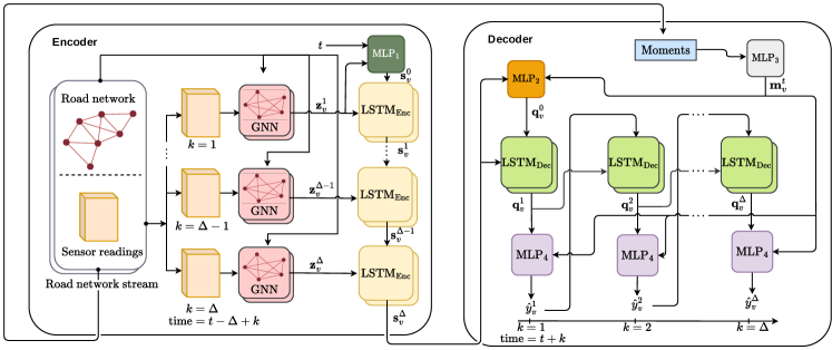
At an individual node level, the proposed problem is a sequence-to-sequence regression task, wherein we feed the time-series over past snapshots and forecast the future time-series on the target node. To model this problem, we use an Encoder-Decoder architecture as outlined in Fig. 2. To jointly capture the spatio-temporal dependency among nodes, the encoder is composed of a stack of siamese Gnns and Lstms, i.e., the weights and architecture are identical across each stack. The number of stacks corresponds to the number of historical snapshots one wishes to train on. Each stack is assigned an index depending on how far back it is from the current time $t$. Due to the siamese architecture, the number of stacks does not affect the number of parameters. In addition, the siamese design allows one to dynamically specify the stack size at inference time in a query-specific manner depending on the amount of data available. For simplicity, we will assume the number of historical snapshots to be the same as the forecasting horizon, which is denoted as $\Delta$.

In the $k^{th}$ stack, where $0\leq k\leq\Delta$, graph snapshot $\mathcal{G}_{t-\Delta+k}$ is passed through the Gnn to learn node representations. The node representation not only characterises its own state, but also the state in its “neighborhood”. The “neighborhood” that affects the time-series of the target node is automatically learned through Lipschitz-gating. Each stack of siamese Lstm in the encoder receives two inputs: the node embedding of the target node corresponding to its timestamp and the Lstm output from the previous stack.

The decoder has a stack of siamese Lstms as well. However, the decoder Lstms have separate weights than the encoder Lstms. The stack size is the same as the forecasting horizon $\Delta$. The output of a decoder Lstm is augmented with the moments (mom, [n. d.]) of the sensor value distribution in neighborhood of the target node, which injects a strong prior to the model and elevates its performance. Finally, this augmented representation is passed through an Mlp to predict the time-series value. The entire architecture is trained end-to-end with mean absolute error (MAE) loss function, as defined in Eq. 1. The $\Psi_{\Theta}\left(v,t+k\>|\>\overrightarrow{\mathcal{G}}_{[1,t]}\right)$ term in Eq. 1 is computed as:

(3) $$\Psi_{\Theta}\left(v,t+k\>|\>\overrightarrow{\mathcal{G}}_{[1,t]}\right)=\hat{y}_{v}^{k}$$

where $k\in[1,\Delta]$ and $\hat{y}_{v}^{k}$, as depicted in Fig. 2, is the predicted output generated through the $k^{th}$ Lstm in the decoder. The next sections detail these individual components.

3.1. Gnn Module of Frigate

In this section, we discuss the architecture of a single stack of Gnn. We use an $L$-layered message-passing Gnn to model node dependencies. In each layer, each node $v$ receives messages from its neighbors. These messages are aggregated and passed through a neural network, typically an Mlp, to construct the representation of $v$ in the next layer.

The simplest aggregation framework would be a MeanPool layer where the aggregated message at $v$ from its neighbors is simply the mean of their representations. However, this approach is too simplistic for the proposed problem. Specifically, a road network is directed, and hence drawing messages only through incoming (or outgoing) edges is not enough. On the other hand, a direction-agnostic message passing scheme by uniformly drawing messages through all incident edges fails to capture traffic semantics. Furthermore, not all edges are equally important. An incoming edge corresponding to an arterial road is likely to have much more impact on an intersection (node) than a road from a small residential neighborhood. Hence, the importance of a road (edge) towards an intersection (node) must be learned from the data, and accordingly, its message should be weighted. To capture these semantics, we formulate our message-passing scheme as follows.

Let $\mathbf{h}^{\ell}_{v}$ denote the representation of node $v$ in layer $\ell\in[0,L]$ of the $k^{th}$ Gnn. Furthermore, the outgoing and incoming neighbors of $v$ are defined as $\mathcal{N}^{out}_{v}=\{u\mid(v,u)\in\mathcal{E}\}$ and $\mathcal{N}^{in}_{v}=\{u\mid(u,v)\in\mathcal{E}\}$ respectively. Now, $h^{\ell+1}_{v}$ is constructed as follows:

(4) $$\mathbf{h}^{\ell+1}_{v} =\sigma_{1}\left(\mathbf{W}^{\ell}_{1}\left(h_{v}^{\ell}\parallel\mathbf{m}^{\ell,out}_{v}\parallel\mathbf{m}^{\ell,in}_{v}\right)\right)\text{, where}$$

(5) $$\mathbf{m}^{\ell,out}_{v} =\textsc{Aggr}^{out}\left(\left\{\mathbf{h}_{u}^{\ell}\mid u\in N^{out}_{v}\right\}\right)$$

(6) $$\mathbf{m}^{\ell,in}_{v} =\textsc{Aggr}^{in}\left(\left\{\mathbf{h}_{u}^{\ell}\mid u\in N^{in}_{v}\right\}\right)$$

$\parallel$ represents the concatenation operation, $\mathbf{W}^{\ell}_{1}\in\mathbb{R}^{3d\times d}$ is a learnable weight matrix; $d$ is the dimension of node representations. More simply, we perform two separate aggregations over the messages received from the incoming and outgoing neighbors. The aggregated vectors are concatenated and then passed through a linear transformation followed by non-linearity through an activation function $\sigma_{1}$. In our implementation, $\sigma_{1}$ is ReLU. By performing two separate aggregations over the incoming and outgoing edges and then concatenating them, we capture both directionality as well as the topology.

The aggregation functions perform a weighted summation, where the weight of a message-passing edge is learned through sigmoid gating over its positional embedding. More formally,

(7) $$\textsc{Aggr}^{out}\left(\left\{\mathbf{h}_{u}^{\ell}\mid u\in N^{out}_{v}\right\}\right) =\sum_{\forall u\in N^{out}_{v}}\beta_{v,u}\mathbf{h}^{\ell}_{u}$$

(8) $$\textsc{Aggr}^{in}\left(\left\{\mathbf{h}_{u}^{\ell}\mid u\in N^{in}_{v}\right\}\right) =\sum_{\forall u\in N^{in}_{v}}\beta_{u,v}\mathbf{h}^{\ell}_{u}$$

(9) $$\beta_{v_{i},v_{j}} =\frac{1}{1+e^{-\omega_{v_{i},v_{j}}}}\text{, where}$$

(10) $$\omega_{v_{i},v_{j}} =\mathbf{w}^{\ell}\cdot\mathbf{L}_{v_{i},v_{j}}+b\text{, where}$$

(11) $$\mathbf{L}_{v_{i},v_{j}} =\sigma_{2}\left(\mathbf{W}^{\ell}_{\mathbf{L}}\left(\left(\mathbf{w}_{\delta}^{T}\cdot\delta(v_{i},v_{j})\right)\parallel\mathbf{L}_{v_{i}}\parallel\mathbf{L}_{v_{j}}\right)\right)$$

Here, $\mathbf{L}_{v}$ denotes the positional embedding of node $v$, whose construction we will discuss in Section 3.1.1. Intuitively, the positional embedding represents the location of a node such that if two nodes are within close proximity in terms of shortest path distance, then their positional embeddings should also be similar. Since, $\mathbf{L}_{v_{i},v_{j}}$ is a function of the positional embeddings of its two endpoints and the spatial distance between them, $\mathbf{L}_{v_{i},v_{j}}$ may be interpreted as the positional embedding of the edge $(v_{i},v_{j})$. The importance of an edge is computed by passing its positional representation through an Mlp (Eq. 11), which is subsequently converted to a scalar (Eq. 10). Finally, the scalar is passed through a sigmoid gate (Eq. 9) to obtain its weight. Here, $\mathbf{w}_{\delta}\in\mathbb{R}^{d_{\delta}}$, $\mathbf{W}^{\ell}_{\mathbf{L}}\in\mathbb{R}^{2d_{L}+d_{\delta}\times d_{\mathbf{L}_{e}}}$ and $\mathbf{w}^{\ell}\in\mathbb{R}^{d_{L_{e}}}$ are learnable weight parameters; $d_{L}$ and $d_{L_{e}}$ are the dimensionality of the positional embeddings of nodes and edges respectively, and $d_{\delta}$ is the dimension of the projection created over edge distance $\delta_{v_{i},v_{j}}$.. $\sigma_{2}$ in Eq. 11 is an activation function to apply non-linearity. $b$ in Eq 10 is the learnable bias term.

Figure 3. The distribution of cars flowing through the edges in the cities of Beijing, Chengdu and Harbin.

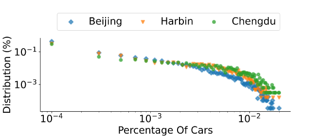
We now discuss the rationale behind this design. In a road network, the distribution of traffic over edges resemble a power-law (Fig. 3). While arterial roads carry a lot of traffic and therefore is a strong determinant of the state of the downstream roads, local roads, which forms the majority, have less impact. Hence, we need to learn this importance of roads from the data. Furthermore, we would like the Gnn to be deep without over-smoothing or over-squashing the representations (Dwivedi et al., 2022). Sigmoid gating serves these dual requirements. First, it assigns a weight to every edge to determine its importance. Second, it enables us to go deep since as more layers are added, we receive messages only from the edges with high weights and therefore avoid over-squashing. Semantically, the roads with high weights should correspond to the arterial roads. Note that unlike Graph attention networks (Veličković et al., 2018), where edges compete among each other for importance (due to normalization in SoftMax), we do not have that effect in a Sigmoid gating. This is more natural for road networks since the magnitude of representations on a busy intersection should be higher than an intersection with no incoming arterial roads. In addition, as we will formally prove in Section 3.4, Sigmoid gating provides higher expressive power. Finally, it is worth noting that the attention weights are directional since it is a function of the positional edge embedding where $\mathbf{L}_{v_{i},v_{j}}\neq\mathbf{L}_{v_{j},v_{i}}$.

Initial embedding of nodes: Let $t$ be the current time and $\Delta$ the number of historical snapshots we are training on. Thus, we will have $\Delta$ stacks of Gnn where the $k^{th}$ Gnn corresponds to snapshot of time $t-\Delta+k,\;k\in[0,\Delta]$ (Recall Fig. 2). The initial embedding of all nodes $v\in\mathcal{V}_{t-\Delta+k}$ in the $k^{th}$ Gnn is defined as:

(12) $$\mathbf{h}^{0,k}_{v}=\left(\mathbf{w}_{\tau}^{T}\cdot\tau^{v}_{t-\Delta+k}\right)\parallel\mathbf{L}_{v}$$

$\mathbf{w}_{\tau}$ is a learnable vector to map the sensor value to a higher dimensional space. $\mathbf{L}_{v}$ is the positional embedding of $v$. Note we do not use the stack index in the notation for $\mathbf{h}^{\ell}_{v}$ (Eq. 4) since all computations are identical except the time-dependent input in Eq. 12. The final output after the $L^{th}$ layer in the $k^{th}$ Gnn is denoted as $\mathbf{z}^{k}_{v}=\mathbf{h}^{L,k}_{v}$.

3.1.1. Positional Embeddings

The simplest approach to encode the position of a node is to embed its latitude and longitude into a higher-dimensional representation. This embedding, however, would not reflect the constraints imposed by the road network. Hence, to learn network-induced positional embeddings, we use Lipschitz embeddings.

Definition 3 (Lipschitz Embedding).

Let $\mathcal{A}=\{a_{1},\cdots,a_{m}\}\subseteq\mathcal{V}$ be a randomly selected subset of nodes. We call them anchors. Each node $v$ is embedded into an $m$-dimensional feature vector $\mathbf{L}_{v}$ where $\mathbf{L}_{v}[i]=\frac{sp(a_{i},v)+sp(v,a_{i})}{2}$, where $sp(u,v)$ is the shortest path distance from $u$ to $v$.

The efficacy of the Lipschitz embedding lies in how well it preserves the shortest path distances among nodes. A well-accepted convention to measure the preservation of distances between the original space and the transformed space is the notion of distortion (Linial et al., 1995).

Definition 4 (Distortion).

Let $X$ be a set of points embedded in a metric space with distance function $d_{X}$. Given a function $f:X\rightarrow Y$ that embeds objects in $X$ from the finite metric space $(X,d_{X})$ into another finite metric space $(Y,d_{Y})$. We define:

(13) $$\text{expansion}(f) =\max_{x_{1},x_{2}\in X}\frac{d_{Y}(f(x_{1}),f(x_{1}))}{d_{X}(x_{1},x_{2})}$$

(14) $$\text{contraction}(f) =\max_{x_{1},x_{2}\in X}\frac{d_{X}(x_{1},x_{2})}{d_{Y}(f(x_{1}),f(x_{2}))}$$

The distortion of an embedding $f$ is defined as the product of its expansion and contraction. If the distortion is $\alpha$, this means that $\forall\,x,y\in X,\;\frac{1}{\alpha}d_{X}(x,y)\leq d_{Y}(f(x),f(y))\leq d_{X}(x,y)$.

In the context of a road network, $X=\mathcal{V}$, and $d_{X}(x_{1},x_{2})$ is the average two-way shortest path distance between $x_{1}$ and $x_{2}$ as defined in Def. 3. Furthermore, the mapping $f:X\rightarrow Y$ is simply the Lipschitz embedding of $X$. Now, to define $d_{Y}(f(x_{1}),f(x_{2}))$, along with dimensionality $m$, we use Bourgain’s Theorem (Linial et al., 1995).

Theorem 1 (Bourgain’s Theorem (Linial et al., 1995)).

Given any finite metric space $(X,d_{X})$, there exists a Lipschitz embedding of $(X,d_{X})$ into $\mathbb{R}^{m}$ under any $L_{p}$ norm such that $m=O(\log^{2}n)$ and the distortion of the embedding is $O(\log n)$, where $n=\lvert X\rvert=|\mathcal{V}|$.

Based on Bourgain’s theorem, if we can show that $d_{X}(u,v)=\frac{sp(u,v)+sp(v,u)}{2}$, as defined in Def. 3, is metric, then choosing $m=O(\log^{2}|\mathcal{V}|)$ anchors and any $L_{p}$ distance in the embedded space would provide a distortion of $O(\log|\mathcal{V}|)$. We next show that $d_{X}(u,v)$ is indeed a metric.

Lemma 1.

$d_{X}(u,v)=\frac{sp(u,v)+sp(v,u)}{2}$ is a metric.

Proof.

See App. E. ∎

The exact algorithm to choose the anchors is described in (Linial et al., 1995). Note that we use the same set of anchors across all snapshots. Since the topology may change across snapshots, the positional embeddings are time-varying as well. Although unlikely, it is possible for an anchor node to get deleted in a particular snapshot. In such a scenario, we denote the distance corresponding to this dimension as $\infty$ for all nodes.

3.2. Encoding Temporal Dependency

To encode long-term temporal dependencies over the node representations, we use an Lstm encoder. Specifically, the final-layer outputs of the Gnn in the $k^{th}$ stack, denoted as $\mathbf{z}^{k}_{v}$, is fed to the $k^{th}$ Lstm stack. In addition, the $k^{th}$ Lstm also receives the hidden state of the $(k-1)^{th}$ Lstm (Recall Fig. 2). Mathematically, the output of the $k^{th}$ Lstm on node $v$, denoted as $\mathbf{s}^{k}_{v}\in\mathbb{R}^{d_{Lenc}}$, is computed as follows.

(15) $$\mathbf{s}^{k}_{v}=\begin{cases}\textsc{Lstm}_{Enc}\left(\mathbf{s}_{v}^{k-1},\mathbf{z}_{v}^{k}\right)&\text{if k>1}\\ \textsc{Lstm}_{Enc}\left(\textsc{Mlp}_{1}\left(t,\mathbf{z}^{k}_{v}\right),\mathbf{z}_{v}^{k}\right)&\text{if k=1}\end{cases}$$

Since $\mathbf{s}^{0}_{v}$ is undefined for the first Lstm, i.e., $k=1$, we make it a learnable vector through the $\textsc{Mlp}_{1}$. The output of the final Lstm stack corresponding to current time $t$ (See Fig. 2), feeds into the decoder. $d_{L_{enc}}$ is the dimension of the Lstm representations.

Lines 1–6 in Alg. 1 summarize the encoder component. Given stream $\overrightarrow{\mathcal{G}}$, current time $t$, and a target node $v$, we extract the subset $\overrightarrow{\mathcal{G}}_{[t-\Delta,t]}\subseteq\overrightarrow{\mathcal{G}}$ where $k$ denotes the number of Gnn-Lstm stacks. The processing starts at $\mathcal{G}_{t-\Delta}$ where the $k^{th}$ Gnn stack embeds $v$ into $\mathbf{z}_{v}^{k}$. Next, $\mathbf{z}_{v}^{k}$ is passed to the $k^{th}$ Lstm. This completes one stack of computation. Iteratively, we move to the $(k+1)^{th}$ stack and the same operations are repeated till $k=\Delta$, after which $\mathbf{s}^{\Delta}_{v}$ (Eq. 15) is fed to the decoder.

Algorithm 1 Frigate forward pass

0: Frigate, stream $\overrightarrow{\mathcal{G}}$, target node $v$, current timestamp $t$, prediction horizon $\Delta$

0: Predicted sensor values $\hat{y}^{v}_{t+1}\dotsc\hat{y}^{v}_{t+\Delta}$

1: $\mathbf{s}_{v}^{0}\leftarrow\textsc{Mlp}_{1}(t,\mathbf{z}_{v}^{1})$

2: $k\leftarrow 1$

3: for all $\mathcal{G}\in\overrightarrow{\mathcal{G}}_{[t-\Delta,t]}$ do

4:    $\mathbf{z}_{v}^{k}\leftarrow\textsc{Gnn}(v)$

5:    $\mathbf{s}_{v}^{k}\leftarrow\operatorname{LSTM}_{\text{Enc}}(\mathbf{s}_{v}^{k-1},\mathbf{z}_{v}^{k})$

6:    $k\leftarrow k+1$

7: $\mathbf{m}_{v}^{t}\leftarrow\textsc{Mlp}_{3}\left(moments\left(\left\{\tau^{t^{\prime}}_{u}\neq\varnothing|t^{\prime}\in[t-\Delta,t],(u,v)\text{ or }(v,u)\in\mathcal{E}^{t^{\prime}}\right\}\right)\right)$

8: $\hat{y}_{0}\leftarrow\textsc{Mlp}_{2}(\mathbf{s}_{v}^{\Delta},\mathbf{m}_{v}^{t})$

9: $\mathbf{q}_{v}^{0}\leftarrow\mathbf{s}_{v}^{\Delta}$

10: for all $k\in[1\dotsc\Delta]$ do

11:    $\mathbf{q}_{v}^{k}\leftarrow\operatorname{LSTM}_{\text{Dec}}(\mathbf{q}_{v}^{k-1},\hat{y}^{k-1}_{v})$

12:    $\hat{y}_{v}^{k}\leftarrow\textsc{Mlp}_{4}(\mathbf{q}_{v}^{k},\mathbf{m}_{v}^{t})$

13: Re-index $\hat{y}^{v}_{k}\mapsto\hat{y}^{v}_{t+k}$

14: return  $\hat{y}^{v}_{t+1},\dots,\hat{y}^{v}_{t+\Delta}$

3.3. Decoder

The decoder is composed of a stack of $\Delta$ (forecasting horizon) siamese Lstms. Assuming $t$ to be the current time, the output of the $k^{th}$ Lstm in the decoder corresponds to the predicted sensor reading at time $t+k$. Each Lstm receives two inputs: (1) the predicted sensor value in the previous timestamp denoted as $\hat{y}_{v}^{k-1}\in\mathbb{R}$ and (2) the hidden state of the previous Lstm, denoted as $\mathbf{q}_{v}^{k-1}\in\mathbb{R}^{d_{dec}}$. Thus, the output of the $k^{th}$ Lstm is expressed as:

(16) $$\mathbf{q}^{k}_{v}=\begin{cases}\textsc{Lstm}_{Dec}\left(\hat{y}_{v}^{k-1},\mathbf{q}_{v}^{k-1}\right)&\text{if k>1}\\ \textsc{Lstm}_{Dec}\left(\textsc{Mlp}_{2}\left(\mathbf{s}^{\Delta}_{v},\mathbf{m}_{v}^{t}\right),\mathbf{s}_{v}^{\Delta}\right)&\text{if k=1}\end{cases}$$

We have a special case for $k=1$, since both $\hat{y}_{v}^{0}$ and $\mathbf{q}_{v}^{0}$ are undefined. Since we assume a setting of partial sensing across nodes, $\tau^{t}_{v}$ may not be available and hence cannot be used to substitute $\hat{y}_{v}^{0}$. To mitigate this situation, $\mathbf{q}_{v}^{k-1}$ is replaced with the output $\mathbf{s}^{\Delta}_{v}$ of the last Lstm in the encoder and $\hat{y}_{v}^{0}$ is estimated through the $\textsc{Mlp}_{4}$. This Mlp takes as input $\mathbf{s}^{\Delta}_{v}$ and a representation of the moments (mom, [n. d.]) of the observed sensor values in the neighborhood of $v$, denoted as $\mathbf{m}^{t}_{v}$. Formally,

Finally, the predicted sensor value $\forall k\in[1,\Delta],\>\hat{y}_{v}^{k}$ is computed as:

(17) $$\hat{y}_{v}^{k}=\textsc{Mlp}_{4}\left(\mathbf{q}_{v}^{k},\mathbf{m}^{t}_{v}\right)$$

Note that instead of directly predicting the sensor value from the Lstm hidden state $\mathbf{q}^{k}_{v}$, we augment this information with statistical information $\mathbf{m}^{t}_{v}$ on the time-series at $v$. This provides a strong inductive bias to the model and elevates its performance, which we will substantiate empirically during our ablation study in Section 4. Lines 7–12 in Alg. 1 summarize the computations in the decoder.

3.4. Theoretical Characterization of Frigate

Fact 1. Frigate is inductive and permuation-invariant.

Discussion. As outlined in Sections 3.1-3.3 and summarized in Table C.1 in Appendix, the parameter-size is independent of the network size, number of snapshots being used for training, forecasting horizon, and the temporal granularity across snapshots. Furthermore, since Frigate uses sigmoid-weighted sum-pool, it is permutation invariant to node set. Consequently, Frigate can inherently adapt to changes in topology or forecast on unseen nodes without the need to re-train from scratch. As outlined in Table 1 and discussed in Sec. 1.1, majority of existing works on spatio-temporal network-constrained forecasting do not satisfy the needs of being inductive and permutation-invariant. $\hfill\square$

We now focus on the expressive power of Frigate. Message-passing Gnns that aggregate messages from their neighbors are no more powerful than 1-WL (Xu et al., 2019). Hence, given nodes $v$ and $u$, if their $\ell$-hop neighborhoods are isomorphic, they will get identical embeddings. Thus, the position of a node plays no role. Methodologies such as DCRNN (Li et al., 2018), STGCN (Yu et al., 2018), or STGODE (Fang et al., 2021), that build on top of these message-passing Gnns will consequently inherit the same limitation. Frigate does not suffer from this limitation.

Lemma 2.

Frigate can distinguish between isomorphic neighborhoods based on positioning.

Proof.

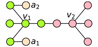
Consider nodes $v_{1}$ and $v_{2}$ in Fig. 4. If we use a 1-layered message-passing Gnn, then their embeddings would be identical since the 1-hop neighborhoods (color coded in green and pink) are isomorphic. Hence, DCRNN, STGCN, or STGODE would not be able to distinguish between them. Frigate augments initial node features with Lipschitz embeddings. Assuming $a_{1}$ and $a_{2}$ to be the anchor nodes, $v_{1}$ would have a Lipschitz embedding of $[2,2]$ vs. $[5,5]$ for $v_{2}$. Hence, Frigate would generate different embeddings for $v_{1}$ and $v_{2}$. ∎

As we will show in our ablation study, removing positional embeddings have a significant impact on the performance.

Lemma 3.

Frigate is at least as powerful as 1-WL.

Proof.

See App. F. ∎

Corollary 1.

Frigate is strictly more expressive than DCRNN, STGCN, and STGODE.

Proof.

This follows naturally by combining Lemmas 2 and 3 since Frigate retains the 1-WL expressivity of DCRNN, STGCN, and STGODE, while also being capable of distinguishing between isomorphic topologies through positional embeddings. ∎

We note that while positional embeddings have been used in the context of Gnns (You et al., 2019; Nishad et al., 2021), they do not provide 1-WL expressivity since messages are exchanged only among anchor nodes. The methodology proposed in this work is therefore unique.

Figure 4. Sample graph to illustrate expressivity of Gnn in Frigate.

Table 2. (a) Data statistics and (b) model size.

(a) Details about the datasets

Dataset	#Nodes	#Edges	Geographical Area (km2)	Mean	Std	Default Seen Percent	#Trips
Beijing (Lian and Zhang, 2018)	28465	64478	16,411	3.22	9.09	5%	785709
Chengdu (che, [n. d.])	3193	7269	14,378	4.54	7.19	50%	1448940
Harbin (Li et al., 2019)	6235	15205	53,068	77.85	124.11	30%	659141

(b) Number of parameters

Model	#Parameters
Frigate	198985
DCRNN	372353
STNN	313906
GraphWavent	247660
STGODE	558582
LocaleGN	333636

4. Experiments

In this section, we benchmark Frigate and establish:

• Prediction Accuracy: Frigate is superior compared to baselines for the task of spatio-temporal forecasting on road networks.

• Ablation study: Through extensive ablation studies, we illuminate the significance of each component of Frigate and provide insights into the critical role they play in the overall performance.

• Robustness: We test the limits of our model to frugality in sensing, graph structure modifications at inference time and resilience to non-uniform temporal granularity across snapshots.

The codebase of Frigate and datasets are available at https://github.com/idea-iitd/Frigate.

4.1. Datasets

We use three real-world datasets collected by tracking the GPS trajectory of taxis. As summarized in Table 2(a), the three datasets correspond to the cities of Beijing, Chengdu and Harbin (Jain et al., 2021). We map-match (Yang and Gidofalvi, 2018) the raw trajectories to their corresponding road networks obtained from Openstreetmap (OpenStreetMap contributors, 2017). The traffic is aggregated into buckets of $5$ minutes and the sensor value corresponds to the number of vehicles passing through each node in a 5-minute interval. From the entire node-set, we select a subset of nodes uniformly at random as the “seen” nodes with installed sensors. Inference and loss calculation is performed only on the unseen nodes. The default percentage of nodes we retain as “seen” is shown in Table 2(a).

(a)

(b)

(c)

Figure 5. Comparison of the distribution of error over nodes grouped by frequency of cars moving through them.

4.2. Experimental Setup

$\bullet$ Computational engine: We use a system running on Intel Xeon 6248 processor with 96 cores and 1 NVIDIA A100 GPU with 40GB memory for our experiments.

$\bullet$ Forecasting horizon: In all the experiments, we choose to predict one hour of traffic information from one hour of historical traffic information. Concretely, since in the datasets the duration between two snapshots is 5 minutes, we set $\Delta=12$. Later, we also simulate what happens if the duration between snapshots is irregular, but even then we have past one hour of data and make predictions of traffic condition up to one hour in the future.

$\bullet$ Evaluation metric: We use mean absolute error (MAE) as the primary metric across all methods (lower is better). We also use sMAPE and RMSE for our key results in Table 3. In addition, we report a $95\%$ confidence interval around the mean by using bootstrapping on the distribution of the metric being used on the “unseen” nodes.

$\bullet$ Training setting: We use a $70$%-$20$%-$10$% train-val-test split for training. This split is on the time dimension. So, to be explicit, during training $70\%$ of the total time series on seen nodes are used. Validation and test are both on different parts of the data both from node perspective and timestep perspective. We stop the training of the model if it does not improve the validation loss for more than 15 epochs. Further, we have varied percentage of training nodes in various experiments to check the fidelity of the FRIGATE, as indicated in the results.

$\bullet$ Baselines: We consider DCRNN (Li et al., 2018), STGCN (Yu et al., 2018), LocaleGN (Li et al., 2022) and STNN (Yang et al., 2021) as our baselines. We adapt GraphWavenet (Wu et al., 2019) and STGODE (Fang et al., 2021) to our setting by removing node embedding matrices or Dynamic Time Warping based graph computation so that they support the triple objectives outlined in Table 1. For all six baselines, we obtain the official code-base released by the authors.

$\bullet$ Parameter settings: We use $16$ anchor nodes to calculate Lipschitz embeddings for all graphs. We use $10$ layers of Gnn in Frigate.

4.3. Inference Accuracy

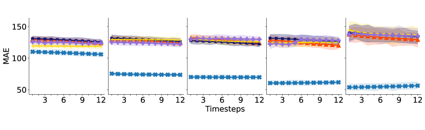
In Table 3, we present the MAE obtained by Frigate and all other baselines on all three datasets. We observe that Frigate consistently outperforms all baselines. On average, the MAE in Frigate is more than 25% lower than the closest baseline. Among the baselines, LocaleGN and STGODE perform the best, followed by DCRNN, followed by GraphWavenet, followed by STNN and then STGCN. We further note that STGCN fails to train on Harbin and Beijing even after 48 hours (the largest dataset evaluated in STGCN (Yu et al., 2018) was of 1026 nodes and it only considered weekday traffic). Likewise, GraphWavenet also fails to train on Harbin and Beijing (the largest dataset evaluated in GraphWavenet (Wu et al., 2019) was of 325 nodes). Now, to better contextualize the results, let us compare the MAE with the standard deviation of sensor values reported in Table 2(a). We observe a clear correlation of MAE with the standard deviation, which explains why all techniques perform comparatively poorer in Harbin. Due to the substantially inferior performance of STGCN and its inability to scale on large datasets, subsequent experiments only consider DCRNN, STNN, STGODE, and LocaleGN as baselines.

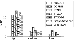
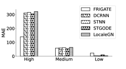
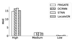
To further diagnose the performance pattern among the benchmarked techniques, we segregate the nodes into three buckets based on the number of cars going through them and plot the distribution of errors within these three buckets. Fig. 5 presents the results. Here, “High”, “Medium” and “Low” corresponds to the top-33 percentile, 33-66 percentile, and bottom-33 percentile, respectively. We derive three key insights from this experiments. First, across all techniques, the MAE reduces as we move towards nodes handling lower traffic. This is natural, since these nodes have low variation in terms of traffic volume. In contrast, high-traffic nodes undergo more fluctuation depending on the time of the day, weekday vs. weekends, etc. Second, we note that Frigate performs better than all other models on high frequency nodes, good on medium frequency nodes, and worse than the rest in low frequency nodes. Overall, it may be argued that doing better in high and medium-frequency nodes are more important since they handle a large majority of the traffic, where Frigate mostly outperforms other techniques. Finally, one of the key reasons of under-performance in DCRNN, STNN, and STGODE is that they over-smooth the high-frequency nodes into inferring lower values as the majority of the nodes are of low-frequency (recall power-law distribution from Fig. 5). Positional embeddings and deep layering through gating enables Frigate to avoid over-smoothing. As we established in Section 3.4, these design choices make Frigate provable more expressive. We further investigate the impact of these two components in our ablation study in Section 4.5.

Table 3. Performance comparison of different approaches for traffic volume prediction. OOT stands for Out of Time and OOM stands for Out of Memory. The lowest MAE (best accuracy), lowest sMAPE and lowest RMSE are highlighted in bold for each dataset.

Model	Dataset	MAE	sMAPE	RMSE
Frigate	Chengdu	$\mathbf{3.547\pm 0.20}$	$\color[rgb]{0,0,0}\mathbf{131.17\pm 3.39}$	$\color[rgb]{0,0,0}\mathbf{5.93\pm 0.31}$
STNN		$5.633\pm 0.18$	$\color[rgb]{0,0,0}199.86\pm 0.00$	$\color[rgb]{0,0,0}9.50\pm 0.50$
DCRNN		$4.893\pm 0.26$	$\color[rgb]{0,0,0}138.17\pm 2.07$	$\color[rgb]{0,0,0}8.10\pm 0.48$
LocaleGN		$\color[rgb]{0,0,0}4.597\pm 0.22$	$\color[rgb]{0,0,0}192.80\pm 0.19$	$\color[rgb]{0,0,0}8.57\pm 0.33$
STGODE		$\color[rgb]{0,0,0}4.693\pm 0.19$	$\color[rgb]{0,0,0}147.12\pm 2.25$	$\color[rgb]{0,0,0}7.72\pm 0.39$
STGCN		$5.712\pm 0.33$	$\color[rgb]{0,0,0}198.38\pm 0.00$	$\color[rgb]{0,0,0}9.47\pm 0.50$
GraphWavenet		$\color[rgb]{0,0,0}5.308\pm 0.30$	$\color[rgb]{0,0,0}147.77\pm 1.81$	$\color[rgb]{0,0,0}8.89\pm 0.43$
Frigate	Harbin	$\mathbf{73.559\pm 2.04}$	$\color[rgb]{0,0,0}\mathbf{93.00\pm 1.89}$	$\color[rgb]{0,0,0}\mathbf{105.01\pm 3.51}$
STNN		$126.305\pm 4.54$	$\color[rgb]{0,0,0}199.68\pm 0.02$	$\color[rgb]{0,0,0}206.91\pm 6.93$
DCRNN		$124.109\pm 5.06$	$\color[rgb]{0,0,0}185.73\pm 0.68$	$\color[rgb]{0,0,0}204.75\pm 6.36$
LocaleGN		$\color[rgb]{0,0,0}128.674\pm 5.10$	$\color[rgb]{0,0,0}169.54\pm 1.43$	$\color[rgb]{0,0,0}207.36\pm 6.58$
STGODE		$\color[rgb]{0,0,0}122.493\pm 4.97$	$\color[rgb]{0,0,0}152.28\pm 1.27$	$\color[rgb]{0,0,0}198.81\pm 6.74$
STGCN		OOT	OOT	OOT
GraphWavenet		OOM	OOM	OOM
Frigate	Beijing	$\mathbf{5.651\pm 0.11}$	$\color[rgb]{0,0,0}\mathbf{169.73\pm 0.45}$	$\color[rgb]{0,0,0}\mathbf{11.87\pm 0.30}$
STNN		$6.215\pm 0.12$	$\color[rgb]{0,0,0}199.99\pm 0.01$	$\color[rgb]{0,0,0}12.82\pm 0.27$
DCRNN		$6.122\pm 0.14$	$\color[rgb]{0,0,0}195.56\pm 0.15$	$\color[rgb]{0,0,0}12.63\pm 0.24$
LocaleGN		$\color[rgb]{0,0,0}5.759\pm 0.13$	$\color[rgb]{0,0,0}172.73\pm 0.33$	$\color[rgb]{0,0,0}12.10\pm 0.03$
STGODE		OOM	OOM	OOM
STGCN		OOT	OOT	OOT
GraphWavenet		OOM	OOM	OOM

(a)

(b)

Figure 6. From left to right, we progressively increase the volume of seen nodes and measure MAE in (a) Chengdu and (b) Harbin. The envelopes signify the 95% confidence bound of the MAEs.

(a)

(b)

(c)

Figure 7. (a) Ablation study. (b) Impact of Gnn layer variations on Chengdu 50% (c) Model resilience to inference time changes on road network topology.

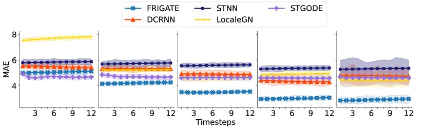
4.4. Impact of Volume of “Seen” Nodes

As in any machine learning task, we expect the accuracy to improve with larger volume of seen nodes. This increases training data, as well as induces a higher likelihood of an unseen node being close to a seen node. Towards that objective, we vary the number of nodes that are “seen” by the models from $10\%$ to $90\%$ of the total number of nodes in the respective road networks and measure MAE against forecasting horizon. Fig. 6 presents the results. We observe that Frigate performs significantly better because of more informative priors and inherent inductivity. Furthermore, the baselines need considerably more data to reach the same performance. For Chengdu, DCRNN trained on 50% of the graph beats our model trained on only 10% of the graph while on Harbin, none of the models ever even surpass our model trained at only 10% of the graph. And as the data increases, the gap between our model and the baselines increases. This economic use of data without losing the ability to generalize is a desirable property that Frigate contains.

Another interesting trend we note is that the performance slightly deteriorates in the baselines from 70% to 90%. It is hard to pinpoint the exact reason. We hypothesize two factors as possible reasons. First, with higher volumes of training data, there is a stronger chance of over-fitting. In addition, we note that the confidence interval expands as the percentage of seen nodes increases since the sample size of test nodes decreases. This trend, which is consistent with statistical theory, means that at low volumes of test sets, the results have higher variability. Frigate does not suffer from this trend, which means it does not overfit. It is well-known in machine learning theory, that tendency to overfit is correlated to the number of parameters. In this regard, we draw attention to Table 2(b), which shows that Frigate has almost 50% and 33% smaller parameter set than DCRNN and STNN, respectively. Also, Frigate utilizes moments as a robust inductive bias, reducing overfitting risks.

4.5. Ablation Study

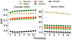
In our ablation study, we systematically turn off various components of Frigate and measure the impact on MAE. Fig. 7(a) presents the results on Chengdu and Harbin.

Gating: Here, we replace the gated convolution with a GraphSAGE layer (Hamilton et al., 2017), leaving rest of the architecture intact. We see a clear increase in MAE indicating the importance of gated convolution layer.

Positional embeddings: To understand its utility on performance, we remove Lipschitz embeddings as features of the node, and thus remove it as an input to the calculation of gating. We see a significant drop in performance, with Chengdu being more pronounced where Lipschitz has the highest drop. This result empirically demonstrates the value of positional embeddings in time-series forecasting on road networks.

In-Out aggregation: In Frigate, we separately aggregate messages from incoming and outgoing neighbors. Here, we measure the impact of aggregating into a single vector. We observe an increase in MAE, showcasing the need for direction-based aggregation.

Moments: We remove the moments from the model and keep everything else in the architecture the same. We see a big drop in performance on both datasets, with Harbin being more pronounced. This establishes the importance of having an informative prior.

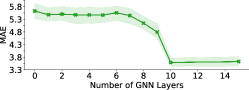
Number of GNN layers: To understand the effect of Gnn layers on performance of Frigate, we vary this parameter while training on Chengdu 50% dataset. As visible in Fig. 7(b), the performance saturates at $10$, which we use as our default value.

4.6. Robustness and Resilience

In this section, we analyze the robustness and resilience of Frigate to changes to network topology and irregular topological sensing. In these experiment, we train Frigate on the original datasets, and then slightly perturb the topology or temporal granularity. We evaluate inference performance on this perturbed dataset. Note that we do not re-train the model after perturbations.

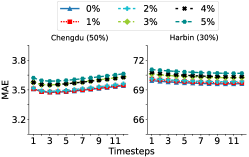
Topology change: To simulate the real-world situation where the road network might change due to road blocks or opening of new roads, we first select the volume of perturbations to be introduced. Assuming this to be $X\%$, we change the network by randomly dropping a maximum of $\frac{X}{2}$% of the edges. In addition, we create an equal number edges among unconnected nodes whose distance is within a threshold. The distances for these edges are sampled, with replacement, from the original distribution of edge distance. We then vary $X$ and measure the impact on MAE. As visible in Fig. 7(c), Frigate is resilient to changes to the road network with minimal drop in accuracy.

Table 4. Impact of irregular temporal granularity on MAE.

Time series	Dataset	MAE
Regular (original)	Chengdu (50%)	$3.547\pm 0.23$
Irregular (perturbed)	Chengdu (50%)	$3.582\pm 0.17$
Regular (original)	Harbin (50%)	$69.700\pm 3.21$
Irregular (perturbed)	Harbin (50%)	$69.834\pm 2.78$

Irregular temporal sensing: In this experiment, we try to break our model by changing the time step granularity at test time. We randomly drop 33.33% of snapshots in $\overrightarrow{\mathcal{G}}_{[t-\Delta,t]}$, effectively reducing the time sequence length and also changing the granularity at which the data is captured. The results are tabulated in table 4, where we observe negligible increase in MAE. The results indicate that the model is resilient to changes in the granularity of snapshots.

5. Conclusion

In this paper, we have proposed a new spatio-temporal Gnn, called Frigate, to forecast network-constrained time-series processes on road networks. We show through experiments on real-world traffic datasets that Frigate significantly outperforms existing baselines. In addition, Frigate is robust to several practical challenges such as partial sensing across nodes, absorb minor updates to road network topology and resilience to irregular temporal sensing. The core competency of Frigate originates from its novel design that incorporates Lipschitz embedding to encode position, sigmoid gating to learn message importance and enable pathways for long-range communication across nodes, directional aggregation of messages, and strong priors in the form of moments of the time-series distribution. In addition, Frigate is built from the ground-up keeping inductivity as a core objective. On the whole, Frigate takes us closer to deployable technology for practical workloads.

Appendix A Notations

Table A.1. Notations used in the paper

Symbol	Meaning
$\overrightarrow{\mathcal{G}}$	The road network stream
$\mathcal{G}_{t}$	Road network snapshot at time $t$
$\overrightarrow{\mathcal{G}}_{[i,j]},\>i\leq j$	$\{\mathcal{G}_{i},\mathcal{G}_{i+1},\dotsc,\mathcal{G}_{j}\}\subseteq\overrightarrow{\mathcal{G}}$
$\mathcal{V}_{t}$	Vertex set at timestep $t$
$\mathcal{V}^{tr}$	Set of vertices to be trained on
$\mathcal{E}_{t}$	Edge set at timestep $t$
$\delta$	Haversine distance function
$\tau_{t}$	Sensor readings $\forall$ nodes at time $t$
$T$	Number of snapshots of the graph
$\Delta$	Prediction horizon: how many timesteps in future to predict
$\Psi_{\Theta}$	The model with parameters $\Theta$
$\mathcal{P}$	Permutation function
$\mathcal{N}(v)$	Set of nodes in the neighborhood of node $v$
$\mathbf{L}_{v}$	Positional embedding of node $v$
$\mathbf{L}_{v_{i},v_{j}}$	Positional embedding of edge $(v_{i},v_{j})$
$\mathbf{h}_{v}^{\ell}$	Intermediate representation of node $v$ at layer $\ell$ in Gnn
$\mathbf{z}_{v}^{k}$	Final representation of node $v$ in $k^{th}$ stack output by Gnn
$\mathbf{s}_{v}^{k}$	Hidden state + cell state of $\operatorname{LSTM}_{\text{Enc}}$ at step $k$
$\mathbf{m}_{v}^{t}$	Representation of moments of $\mathcal{N}(v)$ at time $t$
$\mathbf{q}_{v}^{k}$	Hidden state + cell state of $\operatorname{LSTM}_{\text{Dec}}$ at step $k$
$\hat{y}_{v}^{k}$	Prediction at $k^{th}$ step from $\operatorname{LSTM}_{\text{Dec}}$
$\cdot\|\cdot$	Concatenation operator
$sp(u,v)$	Shortest path between $u$ and $v$
$\lVert\cdot\rVert_{2}$	L2 norm

Appendix B Inference time

The inference times of the three models are shown in Table B.1. Frigate is faster than STNN but slower than DCRNN. However, we note that even though Frigate is slower than DCRNN it is still fast enough to be deployed for real-world workloads.

Table B.1. Inference times

Model	Time(s)
DCRNN	0.0081
STGODE	0.0164
Frigate	0.0207
STNN	0.0375
LocaleGN	0.0492

Appendix C Parameter size

Table C.1. Dimensionality of the parameters used in Frigate.

Parameter	Shape
$\mathbf{W}_{1}^{\ell}$	$\mathbb{R}^{3d\times d}$
$\mathbf{w}_{\delta}^{T}$	$\mathbb{R}^{d_{\delta}}$
$\mathbf{W}_{\mathbf{L}}^{\ell}$	$\mathbb{R}^{2d_{L}+d\delta\times d_{L_{e}}}$
$\mathbf{w}^{\ell}$	$\mathbb{R}^{d_{L_{e}}}$
$\mathbf{w}^{T}_{\tau}$	$\mathbb{R}^{d_{\tau}}$
$\textsc{Mlp}_{1}$	$\mathbb{R}^{d_{Lenc}}$
$\textsc{Mlp}_{2}$	$\mathbb{R}^{d_{dec}}$
$\textsc{Mlp}_{3}$	$\mathbb{R}^{d_{moments}}$
$\textsc{Mlp}_{4}$	$\mathbb{R}^{d_{dec}+d_{moments}}$

Appendix D Other results

Figure D.1. Prediction on Beijing (5%) dataset

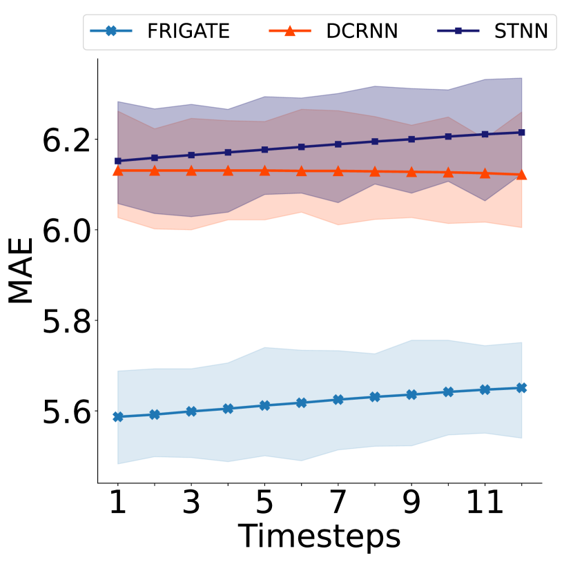
Fig. D.1 shows the MAE of the three models on Beijing (5%) dataset against the prediction horizon.

Appendix E Proof of Lemma 1

See 1

Proof.

We need to show (1) Symmetry: $d_{X}(u,v)=d_{X}(v,u)$, (2) Non-negativity: $d_{X}(u,v)\geq 0$, (3) $d_{X}(u,v)=0$ iff $u=v$ and (4) Triangle inequality: $d_{X}(u,v)\leq d_{X}(u,w)+d_{X}(w,v)$.

We omit the proofs of first three properties since they are trivial. We use proof-by-contradiction to establish triangle inequality.

(18) $$\text{Let us assume }d_{X}(u,v) >d_{X}(u,w)+d_{X}(w,v)$$

$$or,sp(u,v)+sp(v,u) >sp(u,w)+sp(w,u)+sp(w,v)+sp(v,w)$$

From the definition of shortest paths, $sp(u,v)\leq sp(u,w)+sp(w,v)$ and $sp(v,u)\leq sp(v,w)+sp(w,u)$. Hence, Eq. 18 is a contradiction. ∎

Appendix F Proof of Lemma 3

See 3

Proof.

Gin (Xu et al., 2019) is as powerful as 1-WL (Xu et al., 2019). This power is induced by the Sum-Pool aggregation since sum-pool is injective function, i.e., two separate aggregation over messages would be identical if and only if the input messages are identical . Frigate can also model sum-pool, and in the more general case, an injective message aggregation, whenever the sigmoid gate over all edges is some value $x\neq 0$ (Recall Eq. 9). This happens if $\mathbf{w}^{\ell}$ in Eq. 10 is a zero vector, the bias $b$ in Eq. 10 is non-zero and the submatrix in $\mathbf{W}^{1}_{1}$ of Eq. 4 applying linear transformation to Lipschitz embeddings of nodes is $0$. ∎

References

- (1)
- che ([n. d.]) [n. d.]. Gaia Open Dataset. gaia.didichuxing.com.
- mom ([n. d.]) [n. d.]. Moment (Mathematics). https://en.wikipedia.org/wiki/Moment_(mathematics). Accessed: 2023-02-01.
- Bai et al. (2020) Lei Bai, Lina Yao, Can Li, Xianzhi Wang, and Can Wang. 2020. Adaptive graph convolutional recurrent network for traffic forecasting. Advances in neural information processing systems 33 (2020), 17804–17815.
- Chen et al. (2021) Yuzhou Chen, Ignacio Segovia, and Yulia R Gel. 2021. Z-GCNETs: time zigzags at graph convolutional networks for time series forecasting. In International Conference on Machine Learning. PMLR, 1684–1694.
- Dwivedi et al. (2022) Vijay Prakash Dwivedi, Ladislav Rampášek, Mikhail Galkin, Ali Parviz, Guy Wolf, Anh Tuan Luu, and Dominique Beaini. 2022. Long Range Graph Benchmark. In NeurIPS.
- Fang et al. (2021) Zheng Fang, Qingqing Long, Guojie Song, and Kunqing Xie. 2021. Spatial-temporal graph ode networks for traffic flow forecasting. In Proceedings of the 27th ACM SIGKDD Conference on Knowledge Discovery & Data Mining. 364–373.
- Hamilton et al. (2017) Will Hamilton, Zhitao Ying, and Jure Leskovec. 2017. Inductive representation learning on large graphs. Advances in neural information processing systems 30 (2017).
- Jain et al. (2021) Jayant Jain, Vrittika Bagadia, Sahil Manchanda, and Sayan Ranu. 2021. NeuroMLR: Robust & Reliable Route Recommendation on Road Networks. Advances in Neural Information Processing Systems 34 (2021), 22070–22082.
- Joshi et al. (2021) Manas Joshi, Arshdeep Singh, Sayan Ranu, Amitabha Bagchi, Priyank Karia, and Puneet Kala. 2021. Batching and matching for food delivery in dynamic road networks. In 2021 IEEE 37th International Conference on Data Engineering (ICDE). IEEE, 2099–2104.
- Lan et al. (2022) Shiyong Lan, Yitong Ma, Weikang Huang, Wenwu Wang, Hongyu Yang, and Pyang Li. 2022. DSTAGNN: Dynamic Spatial-Temporal Aware Graph Neural Network for Traffic Flow Forecasting. In International Conference on Machine Learning. PMLR, 11906–11917.
- Li et al. (2022) Mingxi Li, Yihong Tang, and Wei Ma. 2022. Few-Sample Traffic Prediction With Graph Networks Using Locale as Relational Inductive Biases. IEEE Transactions on Intelligent Transportation Systems (2022).
- Li and Zhu (2021) Mengzhang Li and Zhanxing Zhu. 2021. Spatial-temporal fusion graph neural networks for traffic flow forecasting. In Proceedings of the AAAI conference on artificial intelligence, Vol. 35. 4189–4196.
- Li et al. (2019) Xiucheng Li, Gao Cong, Aixin Sun, and Yun Cheng. 2019. Learning travel time distributions with deep generative model. In The World Wide Web Conference. 1017–1027.
- Li et al. (2018) Yaguang Li, Rose Yu, Cyrus Shahabi, and Yan Liu. 2018. Diffusion Convolutional Recurrent Neural Network: Data-Driven Traffic Forecasting. In International Conference on Learning Representations (ICLR ’18).
- Lian and Zhang (2018) Jing Lian and Lin Zhang. 2018. One-month beijing taxi GPS trajectory dataset with taxi IDs and vehicle status. In Proceedings of the First Workshop on Data Acquisition To Analysis. 3–4.
- Linial et al. (1995) Nathan Linial, Eran London, and Yuri Rabinovich. 1995. The geometry of graphs and some of its algorithmic applications. Combinatorica 15 (1995), 215–245.
- Liu et al. (2022) Dachuan Liu, Jin Wang, Shuo Shang, and Peng Han. 2022. Msdr: Multi-step dependency relation networks for spatial temporal forecasting. In Proceedings of the 28th ACM SIGKDD Conference on Knowledge Discovery and Data Mining. 1042–1050.
- Medya et al. (2018) Sourav Medya, Sayan Ranu, Jithin Vachery, and Ambuj Singh. 2018. Noticeable network delay minimization via node upgrades. Proceedings of the VLDB Endowment 11, 9 (2018), 988–1001.
- Mitra et al. (2015) Shubhadip Mitra, Sayan Ranu, Vinay Kolar, Aditya Telang, Arnab Bhattacharya, Ravi Kokku, and Sriram Raghavan. 2015. Trajectory aware macro-cell planning for mobile users. In 2015 IEEE Conference on Computer Communications (INFOCOM). IEEE, 792–800.
- Mitra et al. (2017) Shubhadip Mitra, Priya Saraf, Richa Sharma, Arnab Bhattacharya, Sayan Ranu, and Harsh Bhandari. 2017. Netclus: A scalable framework for locating top-k sites for placement of trajectory-aware services. In 2017 IEEE 33rd International Conference on Data Engineering (ICDE). IEEE, 87–90.
- Nishad et al. (2021) Sunil Nishad, Shubhangi Agarwal, Arnab Bhattacharya, and Sayan Ranu. 2021. GraphReach: Position-Aware Graph Neural Network using Reachability Estimations. IJCAI (2021).
- OpenStreetMap contributors (2017) OpenStreetMap contributors. 2017. Planet dump retrieved from https://planet.osm.org . https://www.openstreetmap.org.
- Pande et al. (2017) Shiladitya Pande, Sayan Ranu, and Arnab Bhattacharya. 2017. SkyGraph: Retrieving regions of interest using skyline subgraph queries. Proceedings of the VLDB Endowment 10, 11 (2017), 1382–1393.
- Song et al. (2020) Chao Song, Youfang Lin, Shengnan Guo, and Huaiyu Wan. 2020. Spatial-temporal synchronous graph convolutional networks: A new framework for spatial-temporal network data forecasting. In Proceedings of the AAAI Conference on Artificial Intelligence, Vol. 34. 914–921.
- Veličković et al. (2018) Petar Veličković, Guillem Cucurull, Arantxa Casanova, Adriana Romero, Pietro Lio, and Yoshua Bengio. 2018. Graph attention networks. ICLR (2018).
- Wang et al. (2022) Pengkun Wang, Chaochao Zhu, Xu Wang, Zhengyang Zhou, Guang Wang, and Yang Wang. 2022. Inferring intersection traffic patterns with sparse video surveillance information: An st-gan method. IEEE Transactions on Vehicular Technology 71, 9 (2022), 9840–9852.
- Wang et al. (2018) Yang Wang, Yiwei Xiao, Xike Xie, Ruoyu Chen, and Hengchang Liu. 2018. Real-time Traffic Pattern Analysis and Inference with Sparse Video Surveillance Information.. In IJCAI. 3571–3577.
- Wu et al. (2020) Zonghan Wu, Shirui Pan, Guodong Long, Jing Jiang, Xiaojun Chang, and Chengqi Zhang. 2020. Connecting the dots: Multivariate time series forecasting with graph neural networks. In Proceedings of the 26th ACM SIGKDD international conference on knowledge discovery & data mining. 753–763.
- Wu et al. (2019) Zonghan Wu, Shirui Pan, Guodong Long, Jing Jiang, and Chengqi Zhang. 2019. Graph wavenet for deep spatial-temporal graph modeling. International Joint Conference on Artificial Intelligence 28 (2019).
- Xu et al. (2019) Keyulu Xu, Weihua Hu, Jure Leskovec, and Stefanie Jegelka. 2019. How powerful are graph neural networks? ICLR (2019).
- Yang and Gidofalvi (2018) Can Yang and Gyozo Gidofalvi. 2018. Fast map matching, an algorithm integrating hidden Markov model with precomputation. International Journal of Geographical Information Science 32, 3 (2018), 547–570.
- Yang et al. (2021) Song Yang, Jiamou Liu, and Kaiqi Zhao. 2021. Space Meets Time: Local Spacetime Neural Network For Traffic Flow Forecasting. In 2021 IEEE International Conference on Data Mining (ICDM). IEEE, 817–826.
- Yawalkar and Ranu (2019) Pranali Yawalkar and Sayan Ranu. 2019. Route recommendations on road networks for arbitrary user preference functions. In 2019 IEEE 35th International Conference on Data Engineering (ICDE). IEEE, 602–613.
- You et al. (2019) Jiaxuan You, Rex Ying, and Jure Leskovec. 2019. Position-aware Graph Neural Networks. In ICML, Kamalika Chaudhuri and Ruslan Salakhutdinov (Eds.), Vol. 97. 7134–7143.
- Yu et al. (2018) Bing Yu, Haoteng Yin, and Zhanxing Zhu. 2018. Spatio-temporal graph convolutional networks: A deep learning framework for traffic forecasting. International Joint Conference on Artificial Intelligenc 27 (2018).
- Zheng et al. (2020) Chuanpan Zheng, Xiaoliang Fan, Cheng Wang, and Jianzhong Qi. 2020. Gman: A graph multi-attention network for traffic prediction. In Proceedings of the AAAI conference on artificial intelligence, Vol. 34. 1234–1241.
- Zhou et al. (2023) Zhengyang Zhou, Kuo Yang, Wei Sun, Binwu Wang, Min Zhou, Yunan Zong, and Yang Wang. 2023. Towards Learning in Grey Spatiotemporal Systems: A Prophet to Non-consecutive Spatiotemporal Dynamics. In Proceedings of the 2023 SIAM International Conference on Data Mining (SDM). SIAM, 190–198.