Graph Laplacian Learning with Exponential Family Noise

Abstract

A common challenge in applying graph machine learning methods is that the underlying graph of a system is often unknown. Although different graph inference methods have been proposed for continuous graph signals, inferring the graph structure underlying other types of data, such as discrete counts, is under-explored. In this paper, we generalize a graph signal processing (GSP) framework for learning a graph from smooth graph signals to the exponential family noise distribution to model various data types. We propose an alternating algorithm that estimates the graph Laplacian as well as the unobserved smooth representation from the noisy signals. We demonstrate in synthetic and real-world data that our new algorithm outperforms competing Laplacian estimation methods under noise model mismatch.

1 Introduction

Graphs are ubiquitous in our world. From neural systems to molecules, from social networks to traffic flow, these are all composed of objects and their connections which can be naturally represented abstractly as graphs. Studying these graphs and the data on them has been proven to be vital in making progress in these fields (Bullmore & Sporns, 2009; Trinajstic, 2018; Robins et al., 2007; Latora & Marchiori, 2002). Graph signal processing (GSP) provides an elegant framework for studying these geometric objects. GSP analyzes data or signals on irregular domains, generalizing from signals on a regular grid such as time-series, to signals on networks and graphs (Ortega et al., 2018). It extends Fourier analysis to non-Euclidean domains, and serves as the foundation of many other modern geometric machine learning approaches. However, applying these methods requires the graph of the system to be known, which is not the case in many real-world problems. When the graph is unknown, one needs to resort to various graph inference methods (Mateos et al., 2019) in order to apply GSP or other graph machine learning methods.

Learning the graph structure underlying a set of smooth signals is a classical problem in GSP. Well-established methods optimize a graph representation, usually the graph adjacency matrix or the graph Laplacian, so that the total variation of given signals will be minimal on the learned graph (Dong et al., 2016; Kalofolias, 2016; Egilmez et al., 2017; Kumar et al., 2020). However, smooth graph signals are rarely encountered in the real world and one is often required to deal with noisy signals. One way to bypass this problem is to disregard the noise and treat the noisy signals as smooth signals, especially when the noise is assumed to be considerably small. Although such compromises may yield satisfying results, it is not always appropriate to ignore the the noise. Noisy signals in the real world can be discrete, or even binary in extreme cases, e.g. spiking signals of neurons. These noisy signals are nothing like smooth signals, and smoothness is not even properly defined for various data types. New graph learning approaches are necessary when the noise cannot be ignored.

Following the probabilistic interpretation of graph learning from smooth signals (Dong et al., 2016, 2019), we present a straightforward remedy for the smooth model by adding a new layer of hierarchy that overlays the smooth model outputs with appropriate noise distributions. More precisely, we can model the observations by a conditional response distribution whose mean is parameterized by their underlying smooth representation. Selecting different noise distributions can adapt the model to other data types, with the underlying smooth signal representation kept intact for the use of GSP.

In this paper, we study the problem of learning graph Laplacian matrices from data corrupted with various noise. We first generalize a GSP-based framework that generates graph signals with Gaussian noise (Dong et al., 2016) to a versatile framework that is compatible with all exponential family noise. We then propose Graph Learning with Exponential family Noise (GLEN), an alternating algorithm that estimates the underlying graph Laplacian from the noisy signals without knowing the smooth representation. This generalized method provides a unified solution for graph Laplacian learning when the observed data type varies. Furthermore, we extend GLEN to the time-vertex setting (Grassi et al., 2017) to handle data with temporal correlations, e.g., time-series on a network. We demonstrate in synthetic experiments with different graph models that GLEN is competitive against off-the-shelf Laplacian estimation methods under noise model mismatch. Furthermore, we apply GLEN to different types of real-world data (e.g., binary questionnaires, neural activity) to further demonstrate the efficacy of our methods. Note that our goal is to learn rigorous combinatorial graph Laplacian matrices, which is different from previous work that aims to learn general precision matrices (Biswas et al., 2016; Chiquet et al., 2019).

In summary, our contributions are as follows:

1. We establish a generalized GSP-based framework that models graph signals of different data types using exponential family distributions;

2. We propose an alternating algorithm for joint graph learning and signal denoising under this generalized framework;

3. We also extend our framework to temporally correlated signals using the time-vertex formulation.

2 Background

2.1 Preliminaries

We begin with standard notations. Consider a weighted undirected graph $G=\{\mathcal{V},\mathcal{E},W\}$ , where $\mathcal{V}$ denotes the set of $N$ vertices, $\mathcal{E}$ the set of edges and $W\in\mathbf{S}\mathbb{R}_{+}^{N\times N}$ the weighted adjacency matrix. Each entry $W_{ij}=W_{ji}\geq 0$ corresponds to the weight of edge $\mathcal{E}_{ij}$. Let $D$ denote the diagonal $N\times N$ weighted degree matrix, such that the diagonal entry $D_{ii}=\sum_{j}W_{ij}$ is the degree of node $\mathcal{V}_{i}$. The combinatorial Laplacian matrix $L$ of graph $G$ is given by $L=D-W$.

A real graph signal is a function $f:\mathcal{V}\rightarrow\mathbb{R}^{N}$ that assigns a real value to each vertex of the graph. The definition of a smooth signal varies across different contexts, but generally a smooth graph signal $x$ can be seen as the result of applying a low-pass graph filter $\mathcal{F}(L)$ to a non-smooth signal $x_{0}$

$$x=\mu+\mathcal{F}(L)x_{0}=\mu+\sum_{i}u_{i}f(\lambda_{i})u_{i}^{T}x_{0},$$ (1)

where $\mu\in\mathbb{R}^{N}$ is an offset vector and applying the graph filter relies on $\{u_{i},\lambda_{i}\}$, the eigenvector-eigenvalue pairs of $L$. When $x_{0}\sim\mathcal{N}(0,I_{N})$, the smooth signal follows the distribution

$$x\sim\mathcal{N}(\mu,{\mathcal{F}(L)}^{2}).$$ (2)

This GSP formulation of applying a low-pass filter to white $x_{0}$, as well as different choices of the filter have been well-summarized by Kalofolias (2016).

2.2 Graph Inference from Smooth Signals

Consider a dataset $X\in\mathbb{R}^{N\times M}$, where each row corresponds to one of the $N$ nodes of the graph and each of the $M$ columns contains an independent smooth graph signal $X_{\cdot j}\in\mathbb{R}^{N}$. Suppose the graph $G$ does not change across columns, the goal of graph inference is to learn $G$ so that the columns of $X$ will be smooth on the graph that we learn. As the Laplacian matrix $L$ is uniquely determined by the structure of the graph and the weights of $W$, this problem is equivalent to learning $L$.

Methods of this type can be summarized by the following optimization problem:

$$\min_{L\in\mathcal{L}}\left\{\operatorname{Tr}(X^{T}LX)+\alpha h(L)\right\},$$ (3)

where $\mathcal{L}$ is the space of valid graph Laplacian matrices

$$\mathcal{L}=\left\{L\in\mathbf{S}_{+}^{N}\ |\ L\mathbf{1}=0,L_{ij}=L_{ji}\leq 0,\forall i\neq j\right\},$$ (4)

$h(L)$ is a regularization term, and $\alpha$ is a trade-off parameter. The first term of (3) is known as the graph Laplacian quadratic form, which measures the overall smoothness of graph signals. The smoothness term can be formulated in various ways, resulting in different optimization solutions for different methods. The smoothness term naturally arises when we choose $\mathcal{F}(L)=\sqrt{L^{\dagger}}$ in (1), where $L^{\dagger}$ is the pseudo-inverse of $L$. The second term imposes additional priors on the graph Laplacian, such as connectivity, sparsity, etc., whose specific choice varies across different methods.

Here we briefly describe some popular graph learning methods with smooth signals. Both Hu et al. (2015) and Dong et al. (2016) use the original smoothness term and choose the regularization term $h(L)$ to be the Frobenius norm of $L$ with an additional trace equality constraint. They formulate the problem as a quadratic program with linear constraints and solve it through interior-point methods. Kalofolias (2016) reformulates the smoothness term as $\|W\circ Z\|=\frac{1}{2}\operatorname{Tr}(X^{T}LX)$, where $Z\in\mathbb{R}^{N\times N}$ is the squared Euclidean distance matrix across rows of $X$ and $\circ$ denotes the Hadamard product. They adapt the previous Frobenius norm regularization with a logarithmic barrier to promote connectivity, and solve for $W$, instead of $L$, with primal-dual optimization. Finally, Egilmez et al. (2017) use a different smoothness term and propose to solve

$$\min_{L\in\mathcal{L}}\left\{\operatorname{Tr}(LS)-\log{\det(L)}+\alpha{\|L\circ H\|}_{1}\right\},\$$ (5)

where $S$ is a data statistic and the design of $H$ imposes different regularization on $L$. The problem is solved using block coordinate descent on the rows and columns of $L$. The statistic $S$ is commonly chosen to be the empirical covariance matrix, which makes the first term a scaled smoothness term since $\frac{1}{N-1}\operatorname{Tr}(LXX^{T})=\operatorname{Tr}{(LS)}$.

2.3 Graph Inference with Gaussian Noise

Given a dataset $X$ of corrupted graph signals,  Dong et al. (2016) modeled noisy observations as underlying smooth representations $y$ with additive isotropic Gaussian noise $\epsilon$. Since smooth representations follow a Gaussian distribution, as shown in Eq. (1), the noisy observations also follow a Gaussian distribution

$$x\sim\mathcal{N}(\mu,{\mathcal{F}(L)}^{2}+\sigma_{\epsilon}^{2}I_{N}),$$ (6)

where $\sigma_{\epsilon}$ is the standard deviation of Gaussian noise $\epsilon$ and $\mathcal{F}(L)=\sqrt{L^{\dagger}}$. When $\mu=0$, the MAP estimation of unobserved smooth representation $y$ from (6) amounts to

$$\min_{y}\left\{{\|x-y\|}_{2}^{2}+\beta y^{T}Ly\right\},$$ (7)

where hyper-parameter $\beta$ reflects $\sigma_{\epsilon}^{2}$. Based on (7), Dong et al. (2016) proposed to jointly learn $L$ and the smooth signals $Y$:

$$\min_{L\in\mathcal{L},Y}\left\{{\|X-Y\|}_{F}^{2}+\beta(\operatorname{Tr}(Y^{T}LY)+\alpha h(L))\right\},$$ (8)

where $Y\in\mathbb{R}^{N\times M}$ is the matrix of smooth representations, and $h(L)$ is the same Frobenius norm and trace constraint. To solve Eq. (8), they proposed an alternating algorithm that jointly learns the graph Laplacian and the smooth signal representations: at each iteration they fix one variable and solve for the other. The advantage of this optimization is that each sub-problem objective is convex even though Eq. (8) is not. When $Y$ is fixed ($Y$-step), the problem coincides with the Laplacian learning from smooth signals as in Eq. (3). When $L$ is fixed ($L$-step), solving for $Y$

$$\min_{Y}\left\{{\|X-Y\|}_{F}^{2}+\beta(\operatorname{Tr}(Y^{T}LY))\right\},$$ (9)

enjoys a closed-form solution $Y={(I_{N}+\beta L)}^{-1}X$ that amounts to the Tikhonov filtering of $X$.

3 Graph Inference from Noisy Signals

3.1 Graph Inference with Exponential Family Noise

We first propose a GSP-based framework to model the generative process of noisy signals of different data types, motivated by the Gaussian case. Specifically, the underlying smooth representation is generated from the same process as in (1), which is then connected to the mean parameter of the exponential family distribution through a link function $g$

$$\mathbb{E}[x|y,\mu]=g^{-1}(y+\mu),\ s.t.\ y\sim\mathcal{N}(0,{\mathcal{F}(L)}^{2}).$$ (10)

More precisely, we consider exponential family distributions of the following form

$$p(x|\eta)=k(x)\exp{\{\eta^{T}T(x)-A(\eta)\}},$$ (11)

specified by natural parameters $\eta$, sufficient statistics $T(x)$, and the cumulant generating function $A(\eta)$, which corresponds to the normalization factor of the probability distribution. We list common examplesin Tab. 3 in the Appendix. Then the response model of noisy signals are given by

$$p(x|y,\mu) =k(x)\exp{\{(y+\mu)T(x)-A(y+\mu)\}},$$ (12)

$$s.t.\ y\sim\mathcal{N}(\mu,{\mathcal{F}(L)}^{2}).$$

In reminiscence of generalized linear models (GLMs), we let smooth signals only control the mean parameters through the link function $g$ so that (10) holds.

When $p(x|y,\mu)$ takes some specific exponential family distribution, $p(x)$ can find close relatives in the distribution zoo. For example, when the response is Poisson and the link function is logarithmic, $p(x)$ can be considered as an improper Poisson-Log-Normal (PLN) distribution (Aitchison & Ho, 1989) with the precision matrix constrained to be a combinatorial graph Laplacian

$$x\sim\mathcal{PLN}(\mu,{\mathcal{F}(L)}^{2}).$$ (13)

Similarly, one can also obtain improper Bernoulli-Logit-Normal distributions or Binomial-Logit-Normal distributions from this framework, just to name a few. Note that although these distributions have been studied, we focus on a particular case where the precision matrix is constrained to be a combinatorial graph Laplacian. Such constraints permit a direction connection to GSP and have not been previously addressed in the literature.

Following (Dong et al., 2016), the MAP estimate of $y$ is

$$\min_{y}\left\{-{(y+\mu)}^{T}T(x)+{\mathbf{1}}^{T}A(y+\mu)+\beta y^{T}Ly\right\}.$$ (14)

Including the regularization terms and rewriting the objective in a matrix form, we obtain the full objective

$$\min_{Y,\mu,L\in\mathcal{L}}\Bigl{\{} -\operatorname{Tr}{((Y^{T}+\mathbf{1}{\mu}^{T})T(X))}+\mathbf{1}^{T}A(Y+\mu{\mathbf{1}}^{T})\mathbf{1}$$

$$+\beta(\operatorname{Tr}{(Y^{T}LY)}+\alpha h(L))\Bigr{\}}$$ (15)

$$\quad\quad\quad s.t.\ Y^{T}\mathbf{1}=\mathbf{0},$$

where we slightly abuse the notation of $A$. Note that we also add a constraint for $Y$ which we explain below. The first two terms form a measure of the fidelity of the inferred smooth representations $Y$ with respect to noisy observation $X$. The last two terms are the same as (3), imposing smoothness and other structural priors on the inferred graph. When the distribution is isotropic Gaussian and $\mu=0$, (3.1) coincides with (8). If the regularization is chosen to be the same as (8), one can fully recover the method in (Dong et al., 2016) for learning the graph from Gaussian observations (Sec. 2.3).

To solve (3.1), we propose GLEN, an alternating optimization algorithm, to learn $L$, $Y$ and $\mu$ for general exponential family distributions, inspired by (Dong et al., 2016). Similarly, although the original problem is not convex with respect to all variables, each sub-problem is convex with respect to a single variable. Within each iteration, we update $L$, $Y$ and $\mu$ sequentially, during which the other two are fixed to their current estimations.

For the update of $L$, since the choice of the exponential family distribution only affects the fidelity terms of (3.1), the $L$-step is unaffected and is equivalent to the smooth signal learning scenario, where we simply replace $X$ in (3) with $Y$

$$\min_{L\in\mathcal{L}}\left\{\operatorname{Tr}(Y^{T}LY)+\alpha h(L)\right\}.$$ (16)

Depending on the choice of regularization $h(L)$, previous methods (Dong et al., 2016; Kalofolias, 2016; Egilmez et al., 2017) can be readily plugged in. In the simulations in Sec. 5 we use the solution in (Egilmez et al., 2017) for learning $L$ for demonstration.

The update of $Y$ can be more challenging. With Gaussian noise, we have shown an analytical solution exists for (9), but this is not true with other exponential family distributions. More importantly, because $L$ is a combinatorial graph Laplacian with first-order intrinsic property $L\mathbf{1}=0$, (3.1) is under-determined with infinite solutions. Consider a set of minimizers $\widehat{y},\widehat{\mu},\widehat{L}$ and an arbitrary scaler $s$, $\widehat{y}+s\mathbf{1},\widehat{\mu}-s\mathbf{1},\widehat{L}$ is also a set of minimizers for (3.1). Therefore, we want $Y$ to satisfy an additional constraint $Y^{T}\mathbf{1}=\mathbf{0}$ to prevent floating $Y$ and $\mu$. Therefore, for the $Y$-step, we instead solve the following constrained optimization problem

$$\begin{gathered}\min_{Y}\Bigl{\{}-\operatorname{Tr}{((Y^{T}+\mathbf{1}{\mu}^{T})T(X))}\\ +\mathbf{1}^{T}A(Y+\mu{\mathbf{1}}^{T})\mathbf{1}+\beta(\operatorname{Tr}{(Y^{T}LY)}\Bigr{\}},\\ s.t.\ Y^{T}\mathbf{1}=\mathbf{0}.\end{gathered}$$ (17)

To solve (17), we apply the Newton-Raphson method with equality constraints to each smooth signal representation $y_{j}=Y_{\cdot j}$. Let the gradient and Hessian of the unconstrained problem be $\nabla_{j}$ and $\nabla_{j}^{2}$, where

$$\nabla_{j} =-x_{j}+A^{\prime}(\mu+y_{j})+\beta Ly_{j},$$ (18)

$$\nabla_{j}^{2} =\textrm{diag}(A^{\prime\prime}(\mu+y_{j}))+\beta L.$$ (19)

The update $\Delta y$ of the constrained problem is given by solution of $v$ in the following linear system.

$$\begin{bmatrix}\nabla_{j}^{2}&\mathbf{1}\\ \mathbf{1}^{T}&0\end{bmatrix}\begin{bmatrix}v\\ w\end{bmatrix}=\begin{bmatrix}-\nabla_{j}\\ 0\end{bmatrix}.$$ (20)

Finally, $\mu$ can be updated via a simple GLM fitting. For each node $\mathcal{V}_{i}$, the update amounts to fitting a GLM (with the same exponential distribution) from invented predictors $\mathbf{1}\in\mathbb{R}^{M}$ to responses $X_{i:}^{T}$ with known offset $Y_{i:}^{T}$. The full algorithm is shown in Alg. 1.

Algorithm 1 Alternating Optimization

  Input: noisy signals $Y$

  Onput: graph Laplacian $L$, smooth signals $X$, bias $\mu$

  repeat

     Initialize $Y$ and $\mu$.

     Solve $L=\operatorname*{arg\,min}_{L\in\mathcal{L}}\left\{\operatorname{Tr}(Y^{T}LY)+\alpha h(L)\right\}$

     for $j=1$ to $M$ do

        Calculate $\nabla_{j}$ and $\nabla_{j}^{2}$ as in (18) and (19)

        Solve $v$ in (20)

        Update $Y_{:,j}\leftarrow Y_{:,j}+\textrm{stepsize}*v$

     end for

     for $i=1$ to $N$ do

        Fit GLM from $\mathbf{1}$ to $X_{i,:}^{T}$ with fixed offset $Y_{i,:}^{T}$

     end for

     Set $\textrm{iter}=\textrm{iter}+1$

     Calculate the loss using (3.1)

  until $\textrm{iter}=\textrm{iter}_{max}$

3.2 Graph Inference with Stochastic Latent Variables

We develop a variant of our method that considers $Y$ as a stochastic latent variable. Since the posterior of a smooth signal representation given its noisy observation $p(y|x)$ is usually not tractable, we use variational approaches and approximate that with an isotropic Gaussian distribution $q(y)$. Denote the mean parameter of each Gaussian distribution $q(y_{j})$ with mean $\bar{y}_{j}$, and fix their covariance to be $\Lambda=\lambda I_{N}$. We then derive the evidence lower bound (ELBO), and use its negation as a stochastic version of Eq. (3.1):

$$\begin{gathered}\min_{\begin{subarray}{c}\bar{Y},\mu\\ L\in\mathcal{L}\end{subarray}}\Bigl{\{}-\operatorname{Tr}{((\bar{Y}^{T}+\mathbf{1}{\mu}^{T})T(X))}+\mathbf{1}^{T}\mathbb{E}_{q(Y)}A(Y+{\mu}{\mathbf{1}}^{T})\mathbf{1}\\ +\beta(\operatorname{Tr}{(\bar{Y}^{T}L\bar{Y})}+N\operatorname{Tr}(L\Lambda)+\alpha h(L))\Bigr{\}},\\ s.t.\ \bar{Y}^{T}\mathbf{1}=\mathbf{0}.\end{gathered}$$

The $L$-step then becomes

$$\min_{L\in\mathcal{L}}\left\{\operatorname{Tr}(\bar{Y}^{T}L\bar{Y})+N\operatorname{Tr}(L\Lambda)+\alpha h(L)\right\}.$$ (21)

This is similar to Eq. (5), since $h(L)$ also contains $-\log{\det(L)}$. Using the same regularization, Eq. (21) can be solved with (Egilmez et al., 2017) using the data statistic $S=YY^{T}+N\Lambda$. The $Y$-step now involves the expectation of $A(Y+\mu\mathbf{1}^{T})$ which reflects the stochasticity of $Y$

$$\begin{gathered}\min_{Y}\Bigl{\{}-\operatorname{Tr}{((\bar{Y}^{T}+\mathbf{1}{\mu}^{T})T(X))}+\\ \mathbf{1}^{T}\mathbb{E}_{q(Y)}A(Y+\mu{\mathbf{1}}^{T})\mathbf{1}+\beta(\operatorname{Tr}{(\bar{Y}^{T}L\bar{Y})}\Bigr{\}},\\ s.t.\ \bar{Y}^{T}\mathbf{1}=\mathbf{0}.\end{gathered}$$ (22)

As we choose $q(y)$ to be Gaussian, some exponential family distributions will enjoy a closed-form $\mathbb{E}_{q(Y)}A(Y+\mu\mathbf{1}^{T})$, while others need to seek approximations. The update of $\mu$ remains the same. We term this variational based approach as GLEN-VI. See details and the full derivation in Appendix D.

3.3 Graph Inference with Temporal Correlation

In the previous section, it is assumed that each column of the input matrix $X$ is an independent graph signal sampled from the 2-layer generative model. This is not always true in practice. A common case is that the columns are correlated, for example, when the data has a natural temporal ordering. In such a scenario, each row of the matrix is a canonical 1-D signal on the nodes, and the whole matrix can then be seen as a multivariate time-varying signal lying on the graph. For example, in neural data analysis, the input is often a count matrix whose rows correspond to neurons and columns correspond to time bins. Then we can model the neurons (rows) as nodes of a graph reflecting their (functional) connectivity, while the columns that are close in time should also exhibit similar firing patterns. Such an assumption of temporal correlation is often useful for GSP.

The Time-Vertex signal processing framework (Grassi et al., 2017; Liu et al., 2019) is specifically designed for this kind of setting. For a time-varying graph signal $X\in\mathbb{R}^{N\times M}$, the time-vertex framework considers a joint graph $J$ which is the Cartesian product of a graph $G$ that underlies the $N$ rows and a temporal ring graph $T$ that underlies the $M$ columns. A smooth signal on this product graph is not only smooth upon $G$, but also enjoys temporal smoothness upon $T$. The joint time-vertex Fourier transform (JFT) is simply applying the graph Fourier transform (GFT) on the $G$ dimension and the discrete Fourier transform (DFT) on the $T$ dimension. It can further be shown that the graph Laplacian quadratic form of a matrix $X$ on $J$ is simply the summation of the quadratic forms along each dimension

$$\operatorname{Tr}{(x^{T}L_{J}x)}=\operatorname{Tr}{(X^{T}L_{G}X)}+\operatorname{Tr}{(XL_{T}X^{T})}$$ (23)

where $x$ is the column-wise vectorization of $X$, and $L_{J}$, $L_{G}$, $L_{T}$ denote the Laplacian of $J$, $G$, $T$.

Here we assume that the underlying representation of the input matrix is smooth on the time-vertex graph $J$. As the temporal graph $T$ is known a priori (modeled as a path graph), learning $G$ is essentially the same as learning $J$. The optimization problem becomes the following:

$$\begin{gathered}\min_{\begin{subarray}{c}Y,\mu,\\ L\in\mathcal{L}\end{subarray}}\Bigl{\{}-\operatorname{Tr}{((Y^{T}+\mathbf{1}{\mu}^{T})T(X))}+\mathbf{1}^{T}A(Y+\mu{\mathbf{1}}^{T})\mathbf{1}\\ +\gamma\operatorname{Tr}{(YTY^{T})}+\beta(\operatorname{Tr}{(Y^{T}LY)}+\alpha h(L))\Bigr{\}}\\ s.t.\ Y^{T}\mathbf{1}=\mathbf{0},\end{gathered}$$ (24)

where $\gamma$ controls the weight of temporal edges in $T$. Similar alternating optimization algorithm can be applied for (24), with the only change being the $Y$-step. Again the new gradient and Hessian of the unconstrained problem are

$$\begin{gathered}\nabla_{j}=\left.-x_{j}+A^{\prime}(\mu+y_{j})+\beta Ly_{j}+\right.\\ \left.\ 2\gamma(2y_{j}-y_{j-1}-y_{j+1})\right.,\end{gathered}$$ (27)

$$\nabla_{j}^{2}=\textrm{diag}(A^{\prime\prime}(\mu+y_{j}))+\beta L+4\gamma I_{N},$$ (28)

and the update $\Delta y$ of the constrained problem is given by Eq. (20). We term our solution GLEN-TV.

4 Related Work

The problem of graph inference has been studied from three different perspectives: statistical modeling, GSP and physically motivated models.

Probabilistic graphical models (PGMs), a graph typically encodes conditional independence between random variables. One important class of PGM is the Gaussian Markov random field (GMRF) (Rue & Held, 2005). The precision matrix of a GMRF determines the underlying graph structure and is often estimated using the well-known graphical Lasso algorithm (Friedman et al., 2008). Other PGMs, such as different variants of GMRFs, discrete Markov random fields and Bayesian networks, also have found their applications in many fields, including but not limited to physics (Cipra, 1987), genetics (Yang et al., 2015; Park et al., 2017), microbial ecology (Kurtz et al., 2015; Biswas et al., 2016; Chiquet et al., 2019) and causal inference (Zhang & Poole, 1996; Yu et al., 2004).

Graph inference methods in GSP typically assume that the observations are results of applying graph filters to some initial signals. Inference methods vary on the assumptions of the graph filters and initial signals. Smoothness of the signals with respect to the graph, as we discussed in Sec. 2.1-2.2, is arguably the most popular assumption (Dong et al., 2016; Kalofolias, 2016; Kalofolias & Perraudin, 2017; Egilmez et al., 2017; Kumar et al., 2020; Saboksayr & Mateos, 2021; Buciulea et al., 2022). Other assumptions include polynomial filters (Segarra et al., 2017; Pasdeloup et al., 2017; Navarro et al., 2020), heat diffusion filters (Thanou et al., 2017; Shafipour et al., 2021), and sparse initial signals (Maretic et al., 2017) or sparse spectral representation (Sardellitti et al., 2019; Humbert et al., 2021).

Interestingly, connections can be made between statistical models and GSP. The precision matrix learned by a PGM, such as a GMRF, is often used as the graph Laplacian, but it typically does not meet the requirement of a valid combinatorial Laplacian, which needs to be first-order intrinsic with non-positive off-diagonal elements. One exception is the class of attractive intrinsic GMRFs, where the precision matrices are improper and restricted to M-matrices so that they share the same properties as combinatorial graph Laplacians. Fitting an improper attractive GMRF to the data (Slawski & Hein, 2015) is then essentially solving the same problem as learning a valid combinatorial graph Laplacian.

We describe our framework using the language of GSP, but show it also admits a PGM-like interpretation. For example, when the noise distribution is selected as Poisson, our framework is closely related to the Poisson-Log-Normal (PLN) model. While graph inference from different data types such as Poisson was explored in the field of PGMs, e.g., Ising models and Poisson graphical models (Yang et al., 2012), it is rarely discussed in the field of GSP where precision matrices are constrained to be combinatorial Laplacians. This paper aims to complete this missing piece of rigorous graph Laplacian learning when noise varies across a broad spectrum of exponential family distributions.

Physically motivated models consider the observations as outcomes of some physical processes. This is however less related to our setting and we refer the interested reader to the comprehensive surveys on graph inference in (Dong et al., 2019; Mateos et al., 2019).

5 Experiments

Method	Erdős-Rényi		Stochastic Block		Watts-Strogatz
	F-score	NMI	F-score	NMI	F-score	NMI
SCGL (Lake & Tenenbaum, 2010)	0.6175	0.1447	0.6568	0.2479	0.6503	0.2810
GLS-1 (Dong et al., 2016)	0.5441	0.0676	0.5640	0.1364	0.6016	0.2153
GLS-2 (Kalofolias, 2016)	0.5981	0.1210	0.6267	0.2674	0.6579	0.3305
CGL (Egilmez et al., 2017)	0.7436	0.3179	0.6849	0.2888	0.7185	0.3849
GLEN	0.7318	0.3202	0.7407	0.3696	0.8553	0.5973
GLEN-VI	0.7220	0.2861	0.7180	0.3320	0.7962	0.4878

Table 1: Numerical comparison of structure prediction. Higher F-score and NMI are better.

Method	Erdős-Rényi			Stochastic Block			Watts-Strogatz
	$\textrm{RE}_{L}$	$\textrm{RE}_{edge}$	$\textrm{RE}_{deg}$	$\textrm{RE}_{L}$	$\textrm{RE}_{edge}$	$\textrm{RE}_{deg}$	$\textrm{RE}_{L}$	$\textrm{RE}_{edge}$	$\textrm{RE}_{deg}$
SCGL (Lake & Tenenbaum, 2010)	0.8867	1.0606	0.8488	0.8343	0.8874	0.8213	0.7966	0.8085	0.7928
GLS-1 (Dong et al., 2016)	0.5121	0.7827	0.4405	0.5718	0.7505	0.5214	0.5189	0.7043	0.4501
GLS-2 (Kalofolias, 2016)	0.6883	0.8885	0.6421	0.6770	0.7968	0.6457	0.7780	0.9577	0.7171
CGL (Egilmez et al., 2017)	0.4275	0.6863	0.3566	0.4578	0.6546	0.3977	0.4070	0.5247	0.3651
GLEN	0.3940	0.7040	0.2982	0.4208	0.6934	0.3252	0.3922	0.5433	0.3352
GLEN-VI	0.3693	0.6189	0.2976	0.3996	0.5991	0.3365	0.3508	0.4804	0.3010

Table 2: Numerical comparison of weight prediction. Lower relative errors are better.

We evaluate GLEN on synthetic graphs as well as multiple real datasets. All experiments are done with MATLAB.

5.1 Synthetic Graphs

We consider three random graph models: 1) Erdős-Rényi model with parameter $p=0.3$; 2) Stochastic block model with two equal-sized blocks, intra-community parameter $p=0.4$ and inter-community parameter $q=0.1$; and 3) Watts-Strogatz small-world model, where we create an initial ring lattice with node degree $2K=4$ and rewire every edge of the graph with probability $p=0.1$. Using each model, we generate 20 random graphs of $N=20$ nodes respectively. The weight matrix $W$ of each graph is randomly sampled from a uniform distribution $U(0.1,2)$, and the unnormalized Laplacian is computed as $L_{u}=D-W$. We then normalize it as $L_{0}=\frac{L_{u}}{\operatorname{Tr}{(L_{u})}}N$ to obtain the ground-truth Laplacian. To generate count signals, we set the offset to:

$$\mu_{i}=\begin{cases}2&1\leq i\leq\lfloor\frac{N}{2}\rfloor\\ -2&\lfloor\frac{N}{2}\rfloor<i\leq N.\end{cases}$$

To demonstrate the efficacy of GLEN, we simulate $M=2000$ count signals with Poisson distribution following (12), and infer the synthetic graphs from these synthetic signals. We use the the GSPBOX (Perraudin et al., 2014) and the SWGT toolbox (Hammond et al., 2011) for graph generation and signal processing. Details of our methods with Poisson distributions are shown in Appendix. B.

The baselines are selected to be leading graph Laplacian learning methods: shifted combinatorial graph Laplacian learning (SCGL) (Lake & Tenenbaum, 2010), graph learning from smooth signals 1 (GLS-1) (Dong et al., 2016), graph learning from smooth signals 2 (GLS-2) (Kalofolias, 2016), and combinatorial graph Laplacian learning (CGL) (Egilmez et al., 2017). Because existing methods are designed for Gaussian distributions, which are rather different from Poisson distribution statistically, pre-processing is required for easing such model mismatch. For SCGL, GLS-1 and GLS-2, we first log-transform then centralize the count matrices: $\log(X+1)-\frac{1}{N}\log(X+1)^{T}\mathbf{1}$. For the baseline CGL, we select the data statistic matrix $S$ as the empirical covariance of $\log(X+1)$. As the experiments will show, it is not a good estimation of $\Sigma$. For all the CGL experiments in this paper, we use $H=2I-11^{T}$ to regularize ${\|L\|}_{1}$, corresponding to type-1 regularization in (Egilmez et al., 2017).

We quantitatively compare our proposed methods with the baselines, in terms of structure prediction and weight prediction. For structure prediction, we report two metrics: F-score and normalized mutual information (NMI). The F-score and NMI evaluate the binary prediction of edge existences given by the inferred Laplacian $L^{*}$, but ignore the weights it learns. We threshold the estimated edge weights with $10^{-4}$ to obtain the binary edge prediction, and calculate the F-score and NMI with respect to the ground-truth binary edge patterns. For weight prediction, we report the relative error (RE) of estimated Laplacians, edges, and degrees against the ground-truth, which reflect both structure and weight prediction. Following (Egilmez et al., 2017), we first normalize the inferred Laplacian $L^{*}$ to obtain $\widehat{L}=\frac{L^{*}}{\operatorname{Tr}{(L^{*})}}N$. The relative error of Laplacian, is then computed as $\textrm{RE}_{L}=\frac{{\|\widehat{L}-L_{0}\|}_{F}}{{\|L_{0}\|}_{F}}$. For relative error of edges, we vectorize the upper triangle of $W$ to obtain $\textrm{vech}(L)\in\mathbb{R}^{(N*(N-1))/2}$, and compute the relative $\ell_{2}$ norm $\textrm{RE}_{edge}=\frac{{\|\textrm{vech}(\widehat{L})-\textrm{vech}(L_{0})\|}_{2}}{{\|\textrm{vech}(L_{0})\|}_{2}}$. For the relative error of degrees, we compute the relative $\ell 2$ norm of the degrees $\textrm{RE}_{deg}=\frac{{\|\textrm{diag}(\widehat{L})-\textrm{diag}(L_{0})\|}_{2}}{{\|\textrm{diag}(L_{0})\|}_{2}}$, where $\textrm{diag}(L)$ is the vector of diagonal elements of Laplacian. For the hyper-parameters selection, we perform a grid search on the parameter space for each method. Details are discussed in Appendix. E.

The quantitative comparison of structure and weight prediction for each graph model is shown in Table. 1 and 2, respectively. We bold the best performance and underscore the second best performance for each metric. As we can see, our methods outperform the baselines on almost all structure prediction metrics and all weight prediction metrics. For structure prediction, both our methods GLEN and GLEN-VI are competitive on Erdős Rényi graphs and substantially superior on stochastic block models and Watt-Strogatz small-world graphs. For weight prediction, our methods, especially GLEN-VI, significantly outperform the baselines on all type of graphs. More detailed results on structure and weight prediction are shown in Appendix. F.

In Fig. 1, we visualize the graph Laplacians learned by the different methods for the Erdős-Rényi model. As we can see, SCGL and both GLS methods fail to recover the structures among the second half of the nodes with negative offsets. Surprisingly, CGL recovers those structures quite successfully even without the knowledge of Poisson distribution, but still underperforms GLEN. The performance gap is more significant on other graph models, which we show in Appendix. G. Only our proposed methods obtain both accurate structure and weight estimation on all graph models.

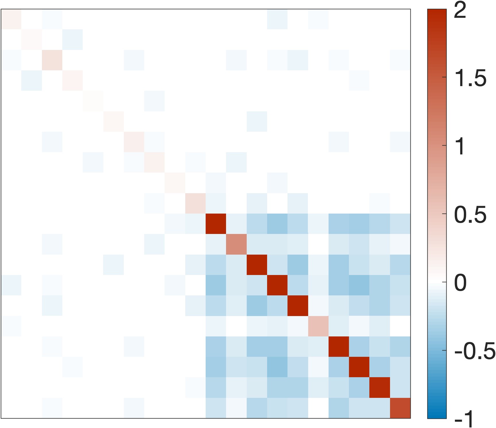
(a) SCGL

(b) GLS-1

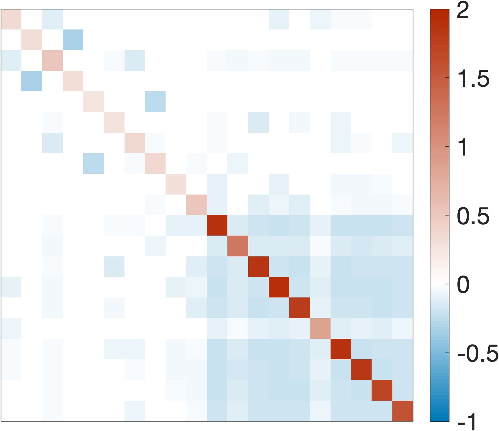
(c) GLS-2

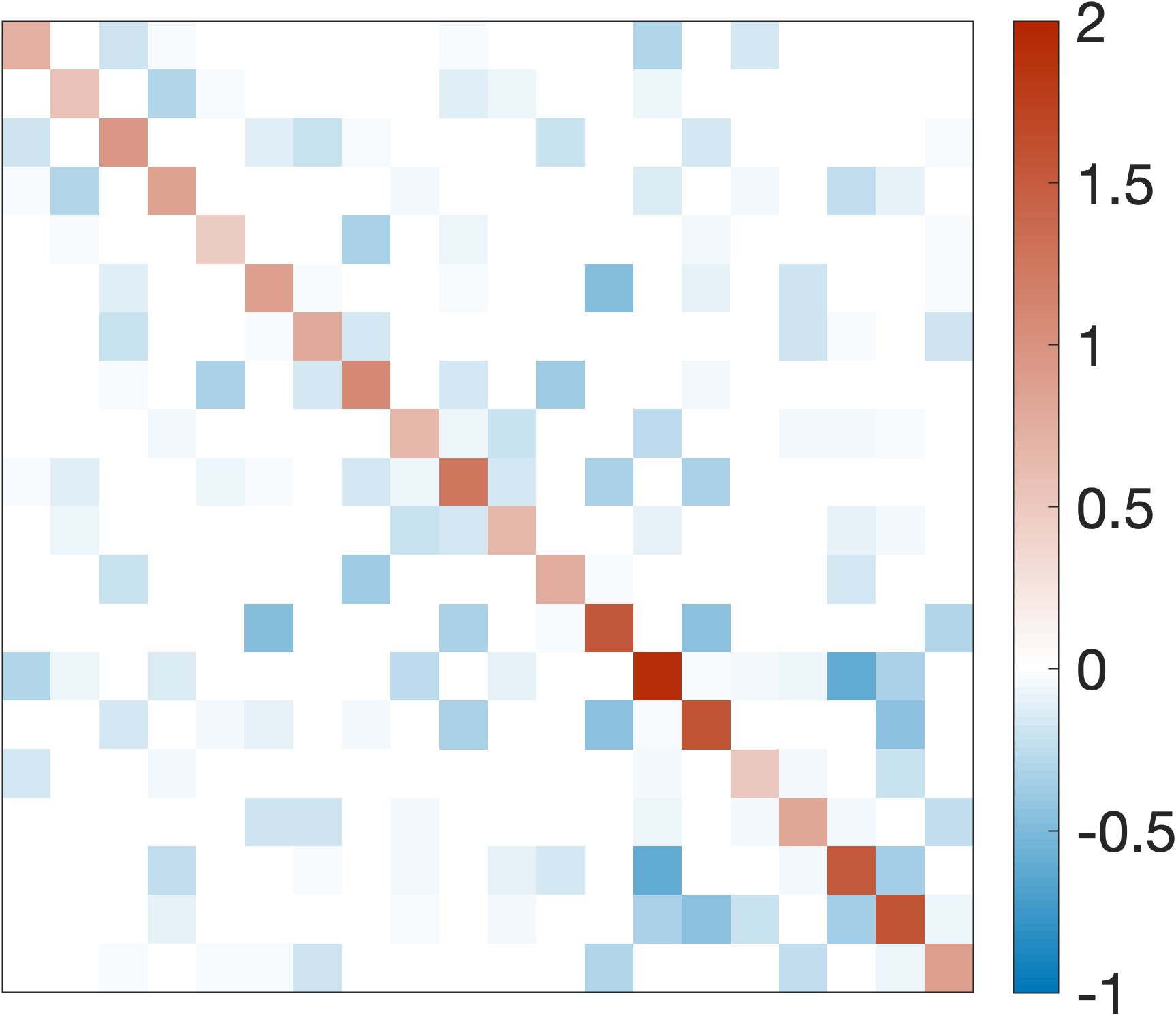
(d) CGL

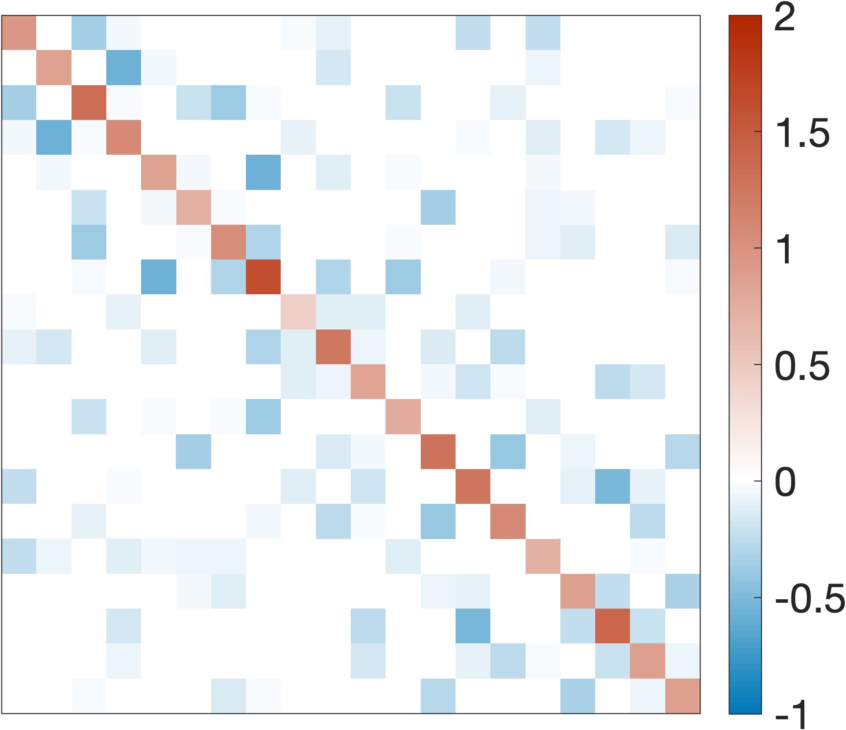
(e) GLEN

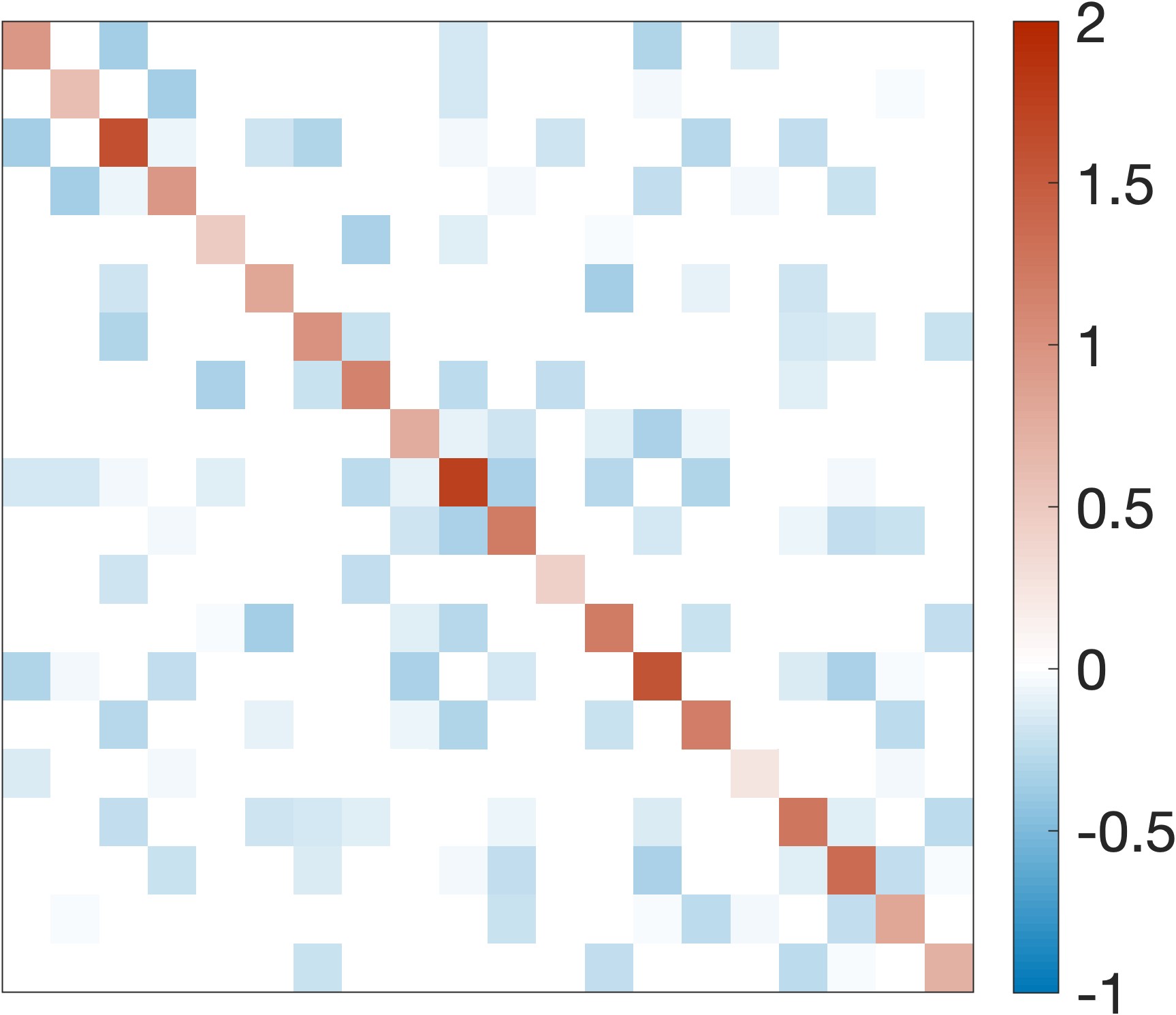
(f) Ground Truth

Figure 1: Normalized graph Laplacians estimated by different methods and the ground truth Erdős-Rényi graph Laplacian (p=0.3). Laplacians are inferred using the weight prediction parameter settings. The red color indicates positive value and the blue indicates negative.

5.2 Chicago Crime Dataset

Now we evaluate GLEN on a real dataset, the Chicago Crime Dataset (Sensors, 2017). Our goal is to learn a graph between different types of crime to reveal their patterns of concurrence. The dataset contains 32 types of crimes that occurred in 77 Chicago communities during every hour from 2001 to 2017. We bin the data by year over the last 10 years and aggregate the count numbers within each bin, resulting in 770 graph signals over 32 crime types. We further remove “Ritualism” from the crimes since there is no occurrence in the 10 years period, resulting in 31 nodes. We apply CGL and GLEN, still with Poisson noise, to this $31\times 770$ count matrix. Evaluating on the Chicago crime dataset demonstrates the importance of considering non-zero offsets, since the average frequency of different types of crime can be very different, and we want to be invariant to the frequency.

We tune the hyper-parameter to encourage sparsity and initialize GLEN with the graph learned by CGL. The crime graphs learned by both methods are shown in Fig. 2. As we can see, the CGL method learns dense weak connections with very few dominant edges. Furthermore, it does not converge when we increase the regularization term to estimate a sparser graph. On the other hand, GLEN improves the CGL estimations and learns a more interpretable sparse graph, better linking similar crimes together.

(a) CGL

(b) GLEN

Figure 2: Graphs (normalized) inferred from the Chicago crime dataset using original CGL and GLEN. Nodes correspond to crime types. Width of edges correspond to the edge weights.

5.3 Animals Dataset

The Animals dataset (Kemp & Tenenbaum, 2008) is a binary matrix of size $33\times 102$. Each row corresponds to an animal species and each column corresponds to a boolean feature such as “has wings?”, “has lungs?”, “is dangerous?”. To learn a graph that represents the similarity between these animals, previous work (Egilmez et al., 2017; Kumar et al., 2020) used a heuristic statistic $S=\frac{1}{d}XX^{T}+\frac{1}{3}I$ suggested by Banerjee et al. (2008) to deal with the binary signals. We instead explicitly model the binary signals using the Bernoulli distribution, resulting in an improper Bernoulli-Logit-Normal model (Aitchison & Shen, 1980), and use GLEN to learn a graph Laplacian. Details can be found in Appendix. C. We compare our results with CGL and plot the learned graphs in Fig. 3. For CGL, we steadily increase the regularization to encourage sparsity so long as the algorithm converges and no isolated node exists. Note that GLEN learns sparser graphs and more clear community structures. Our method also learns meaningful structure that is ignored by CGL, such as the insect sub-network “Bee-Butterfly-Ant-Cockroach”.

(a) CGL

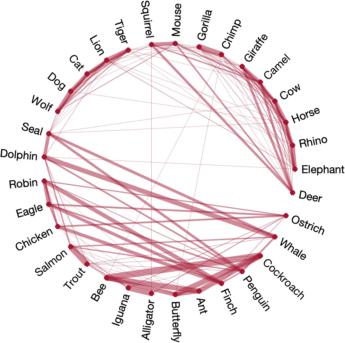
(b) GLEN

Figure 3: Graphs (normalized) inferred from animal dataset using original CGL and GLEN. The nodes correspond to the species. The widths of the edges correspond to the weights of the edges.

5.4 Neural Dataset

We analyze a dataset of neural recordings, $Area2\_Bump$, from the neural latents benchmark (NLB) (Pei et al., 2021), which consists of multiple trials of neural spiking activity and simultaneous behavior data. A macaque controls a cursor to perform center-out reaches towards 1 of 8 target directions, but interrupted by a bump shortly before the reach during some random trials. Neural activity is recorded from the somatosensory area 2 which has been shown to contain information about whole-arm kinematics. A single trial is a non-negative integer matrix $X\in\mathbb{Z}_{+}^{N\times T}$ where each entry $X_{ij}$ counts the firing of neuron $i$ in time bin $j$. Following standard procedure in (Pei et al., 2021), we resample the 1-ms resolution signals into 5-ms bins.

Learning the interactions between the neurons from these spiking activity matrices enables relating functional connectivity patterns to behavior. We infer a graph of neurons for each trial using GLEN-TV with Poisson observations. We perform linear discriminant analysis (LDA) on the degree vector of learned Laplacians, using direction conditions as 8 class labels. LDA achieves $67.86\%$ accuracy which indicates that the structural information in our learned graphs encode the class conditions. When applying GLEN without the temporal modeling, LDA only achieves $61.26\%$ accuracy, which indicates the importance of modeling temporal correlations. We visualize the denoised signals of a single conditions in Fig. 4. See all conditions in Appendix. H.

(a) Average spiking

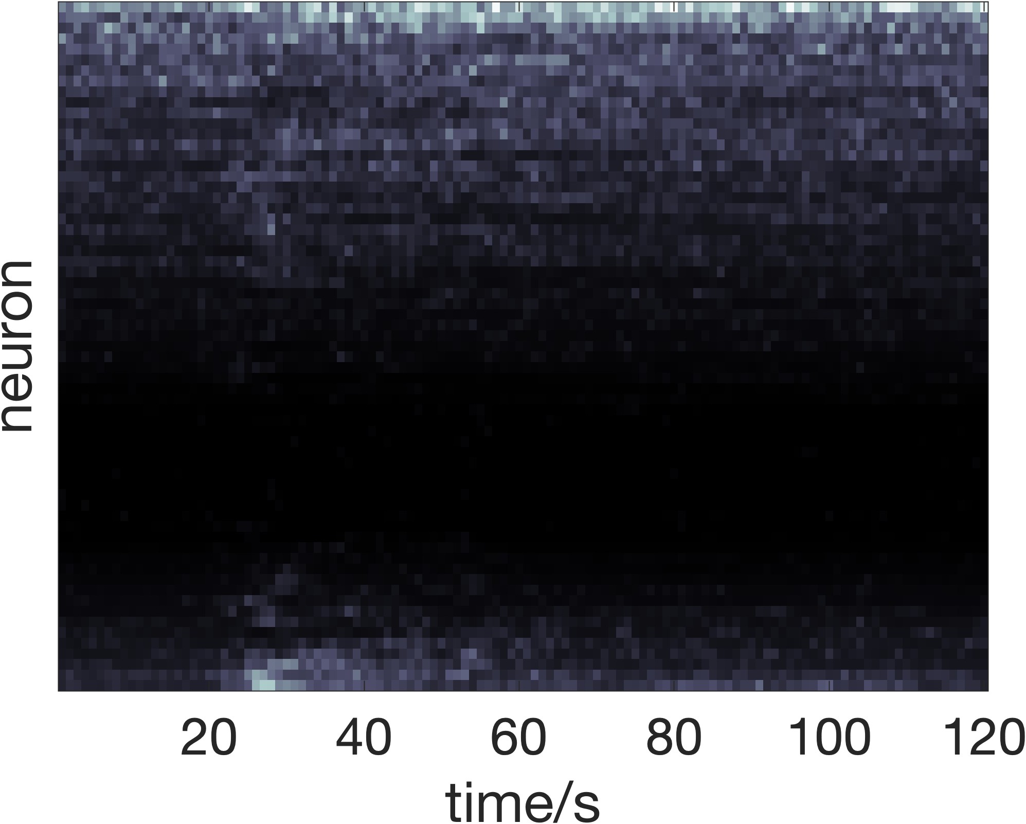
(b) Denoised average signal.

Figure 4: Average spiking from raw count matrix and average denoised signals learned by GLEN-TV, using all bumped trials with target direction $0^{\circ}$.

6 Conclusions

To address the problem of combinatorial graph Laplacian learning from count signals, we proposed a GSP-based generative model that produces signals of different data types from underlying smooth signal representations. We designed GLEN, an alternating method that refines the estimation of the Laplacian and the underlying smooth representations iteratively. We also extended GLEN to the time-vertex framework for learning from time-varying graph signals. We demonstrated that our methods achieve more accurate Laplacian estimation on different synthetic graph models compared to competing approaches, and can learn meaningful graphs on various real datasets. While our experiments highlighted Poisson and Bernoulli distributions, our framework is general for exponential family distributions.

Appendix A Exponential Family Distributions

Although we only conduct experiments with Poisson and Bernoulli distributions, our method is general for all exponential family distributions. Here we list a few common exponential family distribution and their natural link functions for reference in Table. 3. Note that for distributions with multiple parameters, such as Gaussian, we only parameterize the mean of the distribution by smooth signal representations.

Table 3: Exponential family and link functions

Distribution	$\theta$	$\eta$	T(x)	$A(\eta)$	g
Bernouli	$p$	$\log\frac{p}{1-p}$	x	$\log{(1+e^{\eta})}$	logit
Binomial	$p$	$\log\frac{p}{1-p}$	x	$n\log{(1+e^{\eta})}$	logit
Negative Binomial	$p$	$\log p$	x	$-r\log{(1-e^{\eta})}$	logit
Poisson	$\lambda$	$\log\lambda$	x	$e^{\eta}$	log
Gaussian	$[\mu,\sigma^{2}]$	$[\nicefrac{{\mu}}{{\sigma^{2}}},-\nicefrac{{1}}{{2\sigma^{2}}}]$	$[x,x^{2}]$	$\nicefrac{{\mu^{2}}}{{2}}$	identity

Appendix B Derivation of Poisson Observations

We plug-in the Poisson distribution to our framework and derive the corresponding objective functions and the update rules. Given Poisson distribution as shown in Table. 3 and the generalized objective in Eq. (3.1), we obtain the graph learning objective with Poisson noise:

$$\begin{gathered}\min_{Y,\mu,L\in\mathcal{L}}\left\{-\operatorname{Tr}{((Y^{T}+\mathbf{1}{\mu}^{T})X)}+\mathbf{1}^{T}\exp{(Y+\mu{\mathbf{1}}^{T})}\mathbf{1}+\beta(\operatorname{Tr}{(Y^{T}LY)}+\alpha h(L))\right\},\\ s.t.\ Y^{T}\mathbf{1}=\mathbf{0}.\end{gathered}$$ (29)

The gradient and Hessian for unconstrained Newton Ralphson are then given by

$$\nabla_{j} =-x_{j}+\exp{(\mu+y_{j})}+\beta Ly_{j},$$ (30)

$$\nabla_{j}^{2} =\textrm{diag}(\exp{(\mu+y_{j})})+\beta L,$$ (31)

from which the true update $\Delta y_{j}$ is obtained from Eq. (20). For the neural graph inference with Time-Vertex, we plug-in Poisson distribution to Eq. (23) to obtain the objective function

$$\begin{gathered}\min_{Y,\mu,L\in\mathcal{L}}\left\{-\operatorname{Tr}{((Y^{T}+\mathbf{1}{\mu}^{T})X)}+\mathbf{1}^{T}\exp{(Y+\mu{\mathbf{1}}^{T})}\mathbf{1}+\gamma\operatorname{Tr}{(YTY^{T})}+\beta(\operatorname{Tr}{(Y^{T}LY)}+\alpha h(L))\right\},\\ s.t.\ Y^{T}\mathbf{1}=\mathbf{0},\end{gathered}$$ (32)

and the update rules

$$\nabla_{j}=-x_{j}+\exp{(\mu+y_{j})}+\beta Ly_{j}+2\gamma(2y_{j}-y_{j-1}-y_{j+1}),$$ (33)

$$\nabla_{j}^{2}=\textrm{diag}(\exp{(\mu+y_{j})})+\beta L+4\gamma I_{N}.$$ (34)

Appendix C Derivation of Bernoulli Observation

We now plug-in Bernoulli distribution to our framework and derive the corresponding objective functions and the update rules. Given Bernoulli distribution as shown in Table. 3 and the generalized objective in Eq. (3.1), we obtain the graph learning objective with Bernoulli noise

$$\begin{gathered}\min_{Y,\mu,L\in\mathcal{L}}\left\{-\operatorname{Tr}{((Y^{T}+\mathbf{1}{\mu}^{T})X)}+\mathbf{1}^{T}\log(1+\exp{(Y+\mu{\mathbf{1}}^{T})})\mathbf{1}+\beta(\operatorname{Tr}{(Y^{T}LY)}+\alpha h(L))]\right\},\\ s.t.\ Y^{T}\mathbf{1}=\mathbf{0}.\end{gathered}$$ (35)

The gradient and Hessian for unconstrained Newton Ralphson are then given by

$$\nabla_{j} =-x_{j}+\frac{1}{1+\exp{(-\mu-y_{j})}}+\beta Ly_{j},$$ (36)

$$\nabla_{j}^{2} =\textrm{diag}(\frac{1}{\exp{(\mu+y_{j})}+1+\exp{(-\mu-y_{j})}})+\beta L,$$ (37)

from which the true update $\Delta y_{j}$ is obtained from Eq. (20).

Appendix D Derivation of Variational Loss

We now consider the underlying smooth signal representation as latent variables, and derive the evidence lower bound (ELBO) for the variational approach. Following standard procedure, we have the following

$$\mathcal{E}=\log\int p(x|y)p(y)dy=\log\mathbb{E}_{q(y)}[\frac{p(x|y)p(y)}{q(y)}]\geq\mathbb{E}_{q(y)}[\log\frac{p(x|y)p(y)}{q(y)}].$$ (38)

We plug-in $p(x|y)$ given in Eq. (12) and use a Gaussian distribution with mean $\bar{y}$ and covariance $\Lambda$ for $q(y)$

$$\mathcal{E}= \mathbb{E}_{q(y)}[\log\mathbf{1}^{T}k(x)+{(y+{\mu})}^{T}T(x)-\mathbf{1}^{T}A(y+\mu)-\frac{N}{2}\log 2\pi-\frac{1}{2}\log|\Sigma|-\frac{1}{2}y^{T}\Sigma^{-1}y-\log q(y)]$$ (39)

$$= {\mu}^{T}T(x)-\frac{1}{2}\log|\Sigma|+\mathbb{E}_{q(y)}[y^{T}T(x)-\mathbf{1}^{T}A(y+{\mu})-\frac{1}{2}y^{T}\Sigma^{-1}y-\log q(y)]$$ (40)

$$= {\mu}^{T}T(x)+\frac{1}{2}\log|L|+\mathbb{E}_{q(y)}[y^{T}T(x)-\mathbf{1}^{T}A(y+{\mu})-\frac{1}{2}y^{T}Ly-\log q(y)]$$ (41)

$$= {\mu}^{T}T(x)+\frac{1}{2}\log|L|+\bar{y}^{T}T(x)-\mathbf{1}^{T}\mathbb{E}_{q(y)}A(y+{\mu})-\frac{1}{2}\bar{y}^{T}L\bar{y}-\frac{1}{2}Tr(L\Lambda)+\frac{1}{2}\log|\Lambda|$$ (42)

$$= {\mu}^{T}T(x)+\frac{1}{2}\log|L|-\frac{1}{2}Tr(L(\Lambda+\bar{y}\bar{y}^{T}))+\bar{y}^{T}T(x)+\frac{1}{2}\log|\Lambda|-\mathbf{1}^{T}\mathbb{E}_{q(y)}A(y+{\mu})$$ (43)

$$= {({\mu}+\bar{y})}^{T}T(x)-\mathbf{1}^{T}\mathbb{E}_{q(y)}A(y+{\mu})-\frac{1}{2}Tr(L(\Lambda+\bar{y}\bar{y}^{T}))+\frac{1}{2}\log|L|+\frac{1}{2}\log|\Lambda|,$$ (44)

where $\Sigma=L^{\dagger}$. The above objective function is for a single graph signal, we now sum over all graph signals $y_{j}$ and write the above objective function in matrix form with respect to $Y$

$$\mathcal{E}=\operatorname{Tr}{((\bar{Y}^{T}+\mathbf{1}{\mu}^{T})T(X))}-\mathbf{1}^{T}\mathbb{E}_{q(Y)}A(Y+{\mu}{\mathbf{1}}^{T})\mathbf{1}-\frac{1}{2}\operatorname{Tr}{(\bar{Y}^{T}L\bar{Y})}-\frac{N}{2}\operatorname{Tr}(L\Lambda)+\frac{N}{2}\log|L|+\frac{N}{2}\log|\Lambda|.$$ (45)

Note that we constraint that all $q(y_{j})$ have the same covariance $\Lambda$. Once $\Lambda$ is fixed, maximizing Eq. (45) is equivalent to Eq. (46) up to re-weighting. For Poisson distributions, the last expectation term has a closed-form solution

$$\mathbb{E}_{q(y)}A(y+\mu)=\exp{(y+\mu+\frac{1}{2}I_{N}\Lambda)}.$$ (46)

For other exponential family distribution such as Bernoulli, computing this term might need numerical approximation.

In Eq. (46), the mean parameter $y_{j}$ plays a similar role as the smooth signal representation in Eq. (3.1), and $\Lambda_{j}$ accounts for the stochasticity of $y$ which we ignored. For simplicity, we fix $\Lambda_{j}=rI_{N}$. We use $r=0.5$ for the synthetic experiments.

Appendix E Detailed Evaluation Procedure

For the comparison of structure prediction, we perform a grid search on each method’s hyper-parameters, and report the performance of the hyper-parameter setting that achieved the highest average F-score across 20 random graphs. For the comparison of weight prediction, we search through all hyper-parameter settings that produce average F-score within -0.02 range of the highest, and report the performance of the setting with lowest $\textrm{RE}_{L}$ among them. This is because relative error metrics are more sensitive to hyper-parameter settings, meaning that similar structure prediction can have distinct weights. Our evaluation ensures that we can compare different methods by their best weight prediction with reasonably good structure prediction.

Appendix F Detailed Synthetic Results

We report additional metrics of structure and weight prediction. We report the precision and recall of structure prediction for each graph model in Tables. 4-6. For weight prediction, we additionally report the relative error of edge and degree in terms of $\ell 1$ norm, denoted as $\textrm{RE}_{edge}\mbox{-}\ell 1$ and $\textrm{RE}_{deg}\mbox{-}\ell 1$, in Tables. 7-9. The corresponding F-scores of the best weight prediction settings are also shown in the tables. As we can see, GLEN consistently outperforms competing methods.

Method	Precision	Recall	F-score	NMI
SCGL (Lake & Tenenbaum, 2010)	0.5325	0.7378	0.6175	0.1447
GLS-1 (Dong et al., 2016)	0.4141	0.7970	0.5441	0.0676
GLS-2 (Kalofolias, 2016)	0.5014	0.7429	0.5981	0.1210
CGL (Egilmez et al., 2017)	0.7098	0.7846	0.7436	0.3179
GLEN	0.7617	0.7086	0.7318	0.3202
GLEN-VI	0.6591	0.8043	0.7220	0.2861

Table 4: Detailed comparison of structure prediction on Erdős-Rényi graphs (p=0.3).

Method	Precision	Recall	F-score	NMI
SCGL (Lake & Tenenbaum, 2010)	0.5383	0.8457	0.6568	0.2479
GLS-1 (Dong et al., 2016)	0.4433	0.7822	0.5640	0.1364
GLS-2 (Kalofolias, 2016)	0.7753	0.5304	0.6267	0.2674
CGL (Egilmez et al., 2017)	0.5763	0.8557	0.6849	0.2888
GLEN	0.7476	0.7440	0.7407	0.3696
GLEN-VI	0.6378	0.8308	0.7180	0.3320

Table 5: Detailed comparison of structure prediction on stochastic block model (p=0.4, q=0.1).

Method	Precision	Recall	F-score	NMI
SCGL (Lake & Tenenbaum, 2010)	0.5139	0.8863	0.6503	0.2810
GLS-1 (Dong et al., 2016)	0.4720	0.8388	0.6016	0.2153
GLS-2 (Kalofolias, 2016)	0.8215	0.5513	0.6579	0.3305
CGL (Egilmez et al., 2017)	0.5859	0.9338	0.7185	0.3849
GLEN	0.8057	0.9175	0.8553	0.5973
GLEN-VI	0.7385	0.8787	0.7962	0.4878

Table 6: Detailed comparison of structure prediction on Watts-Strogatz small-world graphs (K=2, p=0.1).

Method	F-score	$\textrm{RE}_{L}$	$\textrm{RE}_{edge}\mbox{-}\ell 1$	$\textrm{RE}_{edge}\mbox{-}\ell 2$	$\textrm{RE}_{deg}\mbox{-}\ell 1$	$\textrm{RE}_{deg}\mbox{-}\ell 2$
SCGL (Lake & Tenenbaum, 2010)	0.6055	0.8867	1.3173	1.0606	0.8691	0.8488
GLS-1 (Dong et al., 2016)	0.5292	0.5121	1.1565	0.7827	0.4219	0.4405
GLS-2 (Kalofolias, 2016)	0.5867	0.6883	1.1565	0.8885	0.6422	0.6421
CGL (Egilmez et al., 2017)	0.7383	0.4275	0.6247	0.6863	0.2915	0.3566
GLEN	0.7182	0.3940	0.7107	0.7040	0.2470	0.2982
GLEN-VI	0.7023	0.3693	0.6460	0.6189	0.2483	0.2976

Table 7: Detailed comparison of weight prediction on Erdős-Rényi graphs (p=0.3).

Method	F-score	$\textrm{RE}_{L}$	$\textrm{RE}_{edge}\mbox{-}\ell 1$	$\textrm{RE}_{edge}\mbox{-}\ell 2$	$\textrm{RE}_{deg}\mbox{-}\ell 1$	$\textrm{RE}_{deg}\mbox{-}\ell 2$
SCGL (Lake & Tenenbaum, 2010)	0.6472	0.8343	1.0805	0.8874	0.8441	0.8213
GLS-1 (Dong et al., 2016)	0.5530	0.5718	1.0407	0.7505	0.5153	0.5214
GLS-2 (Kalofolias, 2016)	0.6089	0.6770	1.0112	0.7968	0.6424	0.6457
CGL (Egilmez et al., 2017)	0.6820	0.4578	0.6399	0.6546	0.3363	0.3977
GLEN	0.7226	0.4208	0.6516	0.6934	0.2793	0.3252
GLEN-VI	0.6984	0.3996	0.6327	0.5991	0.2930	0.3365

Table 8: Detailed comparison of weight prediction on stochastic block model (p=0.4, q=0.1).

Method	F-score	$\textrm{RE}_{L}$	$\textrm{RE}_{edge}\mbox{-}\ell 1$	$\textrm{RE}_{edge}\mbox{-}\ell 2$	$\textrm{RE}_{deg}\mbox{-}\ell 1$	$\textrm{RE}_{deg}\mbox{-}\ell 2$
SCGL (Lake & Tenenbaum, 2010)	0.6320	0.7966	1.0347	0.8085	0.8080	0.7928
GLS-1 (Dong et al., 2016)	0.5872	0.5189	0.9655	0.7043	0.4291	0.4501
GLS-2 (Kalofolias, 2016)	0.6482	0.7780	0.9579	0.9577	0.7225	0.7171
CGL (Egilmez et al., 2017)	0.7172	0.4070	0.5152	0.5247	0.2949	0.3651
GLEN	0.8403	0.3922	0.4984	0.5433	0.2887	0.3352
GLEN-VI	0.7885	0.3508	0.4863	0.4804	0.2486	0.3010

Table 9: Detailed comparison of weight prediction on Watts-Strogatz small-world graphs (K=2, p=0.1).

Appendix G Inferred Laplacians

We visualize the ground truth Laplacian of several realizations as well as the inferred Laplacians of different methods in Fig. 5-7. These Laplacians are used for weight prediction. All Laplacians are normalized by their trace.

SCGL	GLS-1	GLS-2	CGL	GLEN	GLEN-VI	Ground Truth

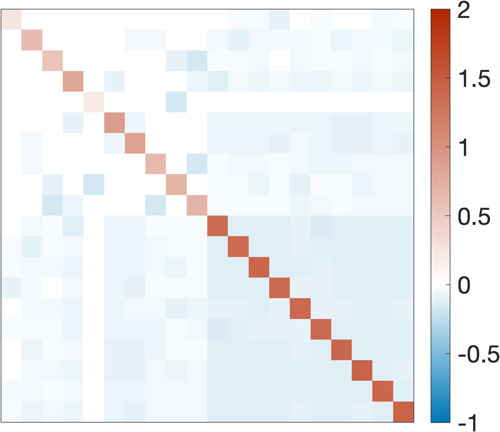
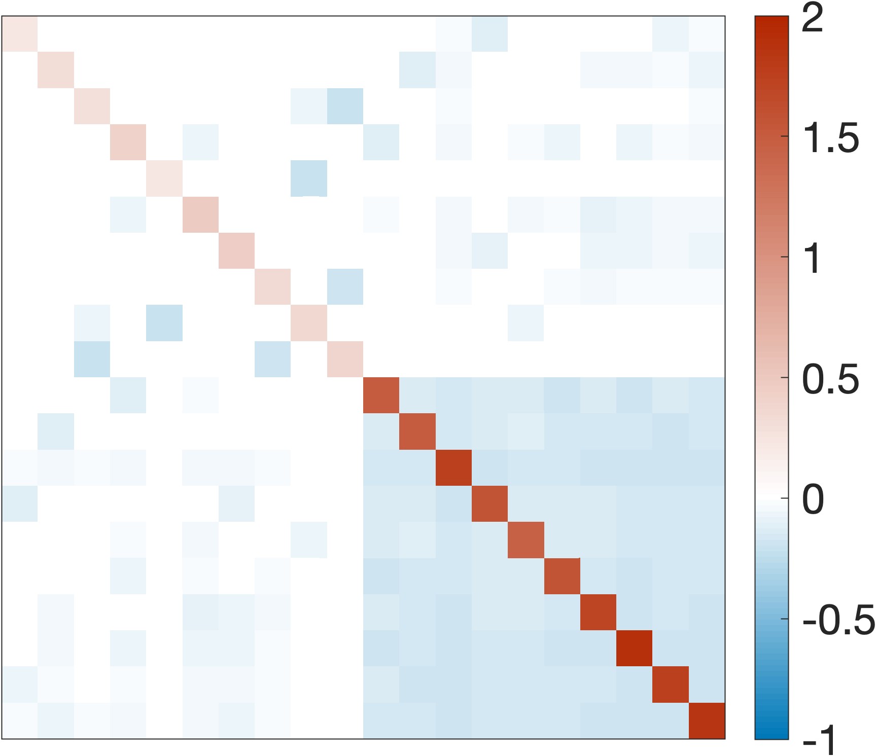
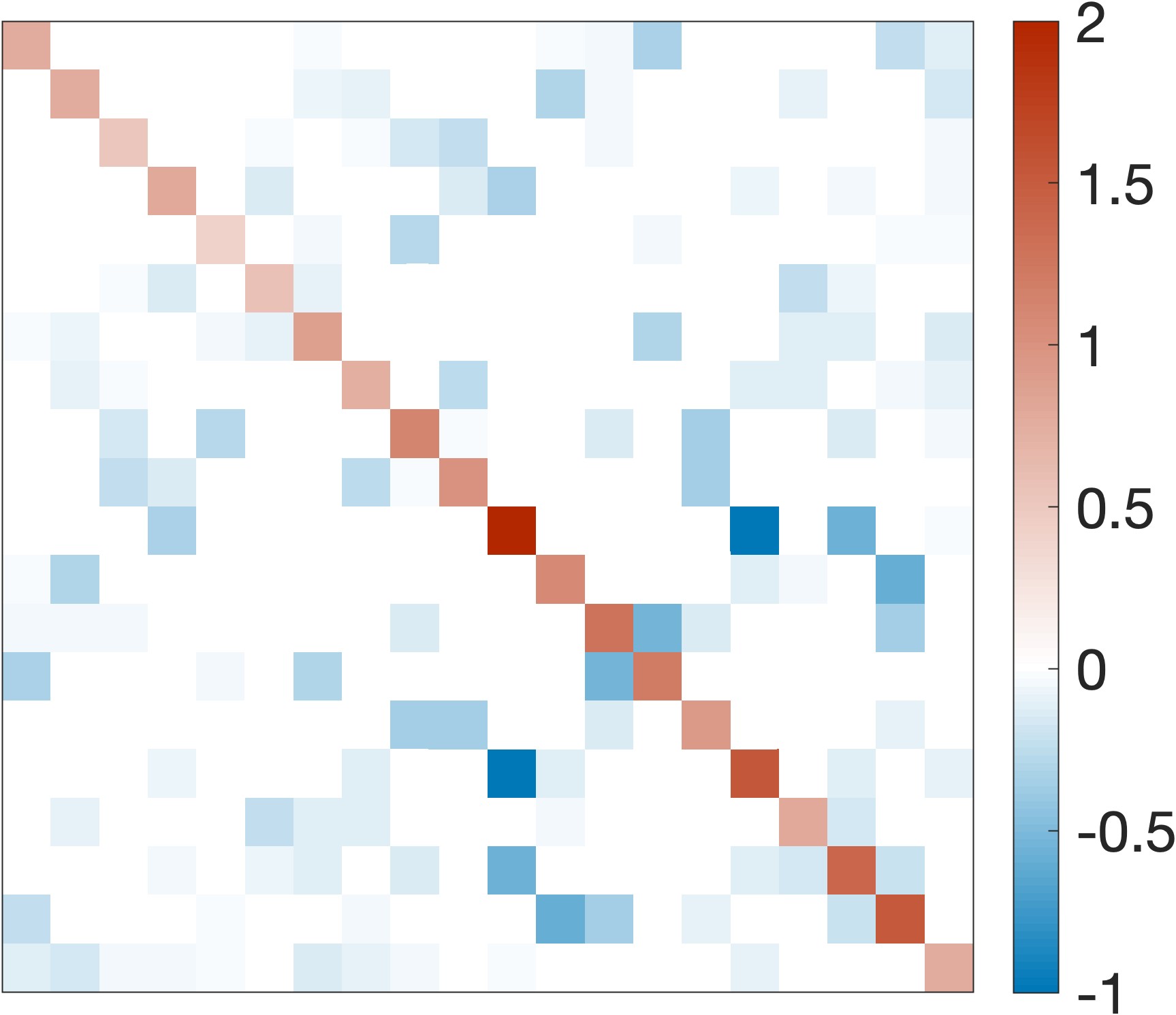
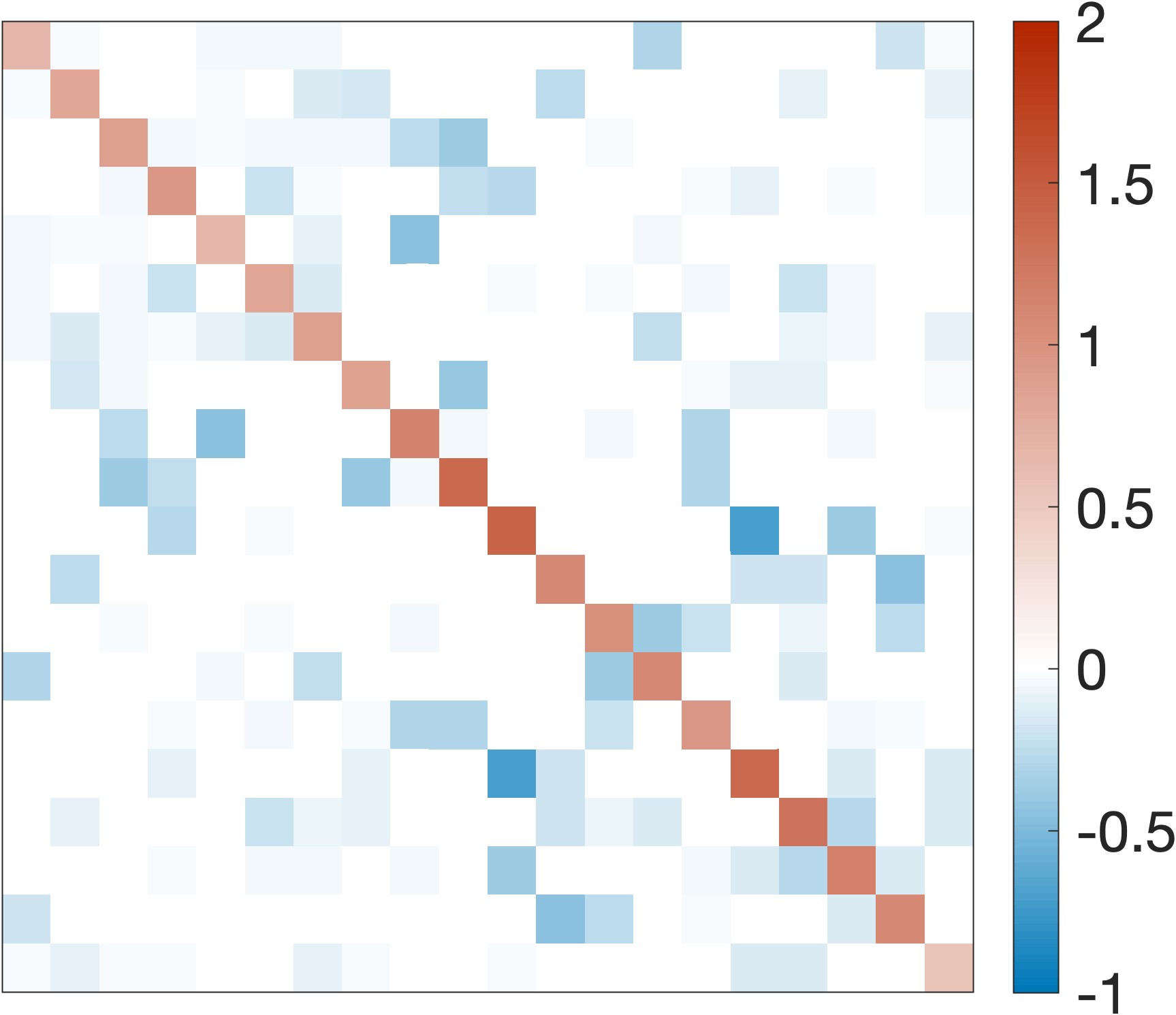
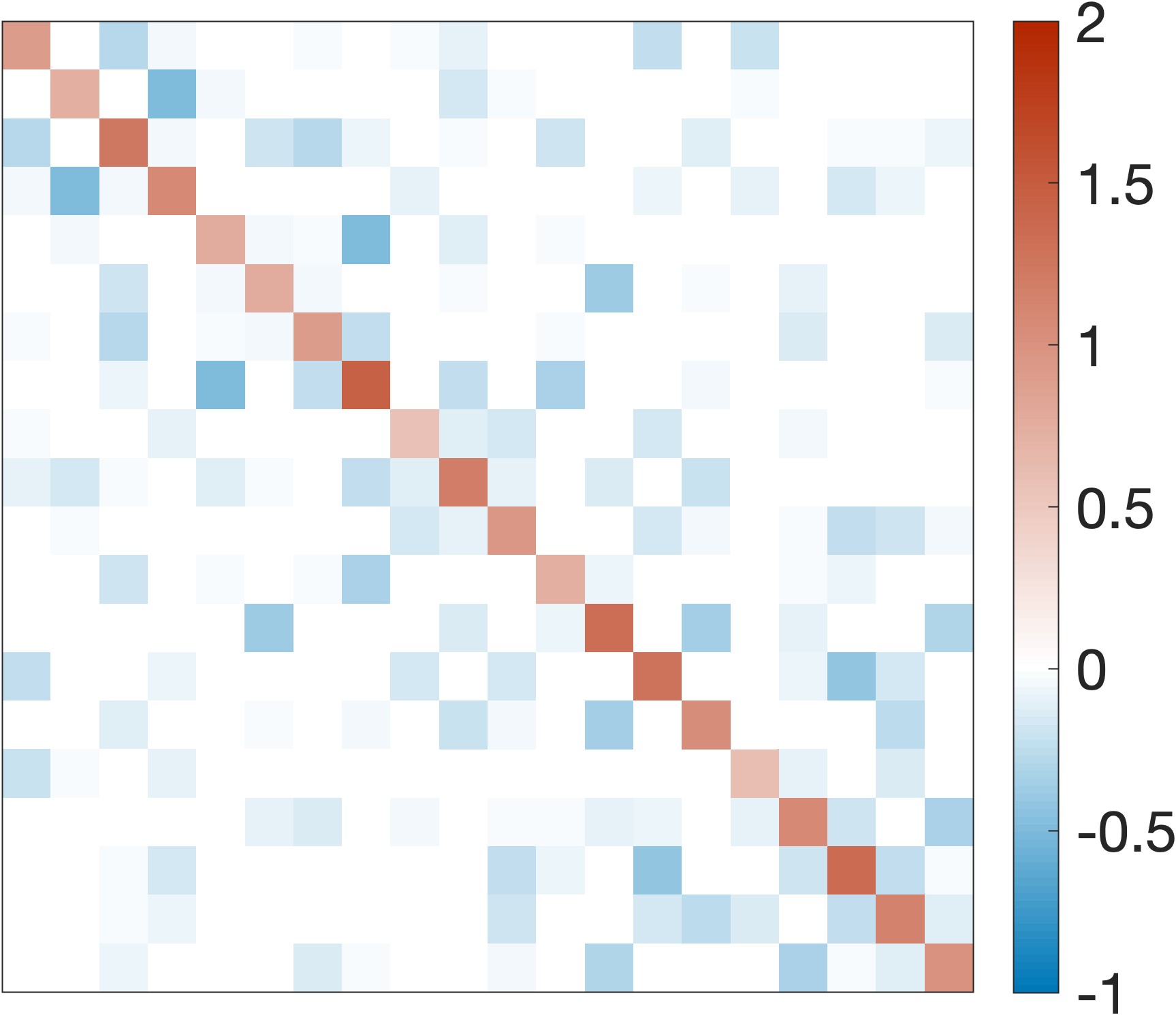
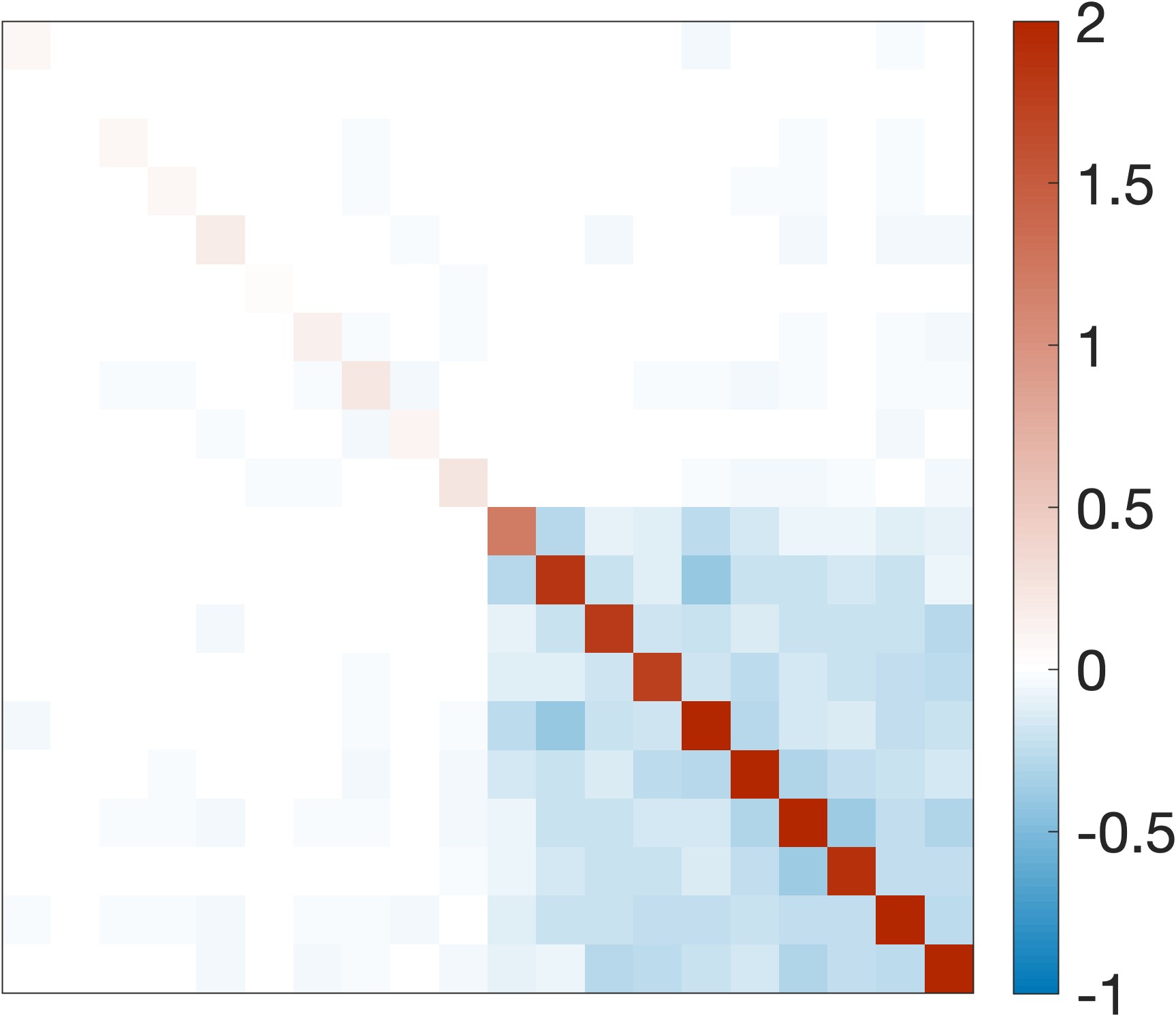
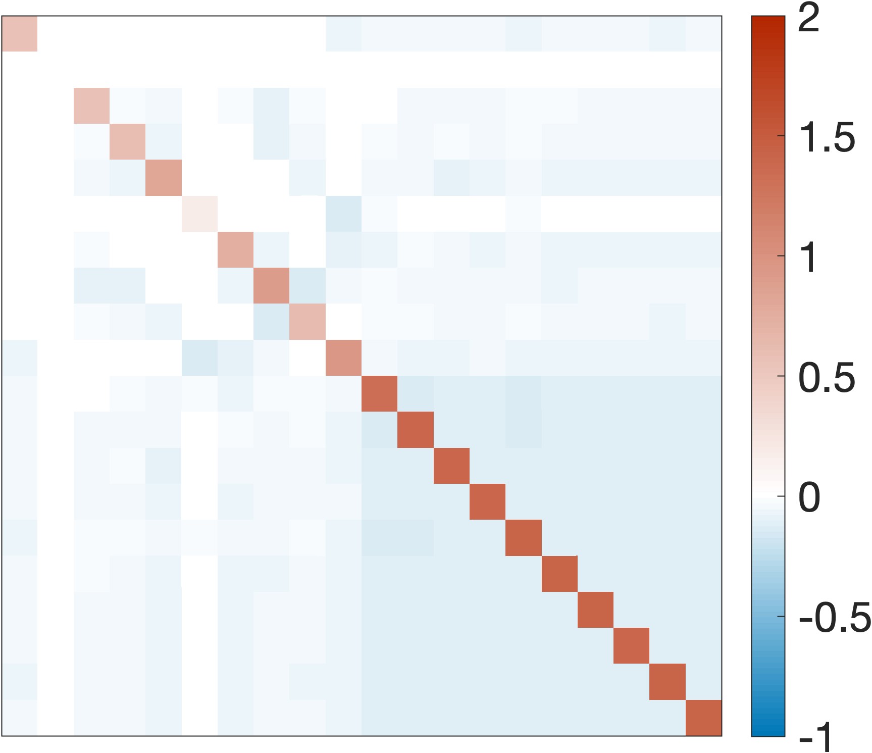
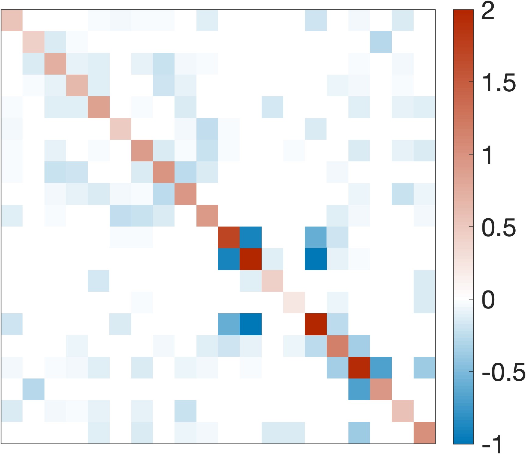
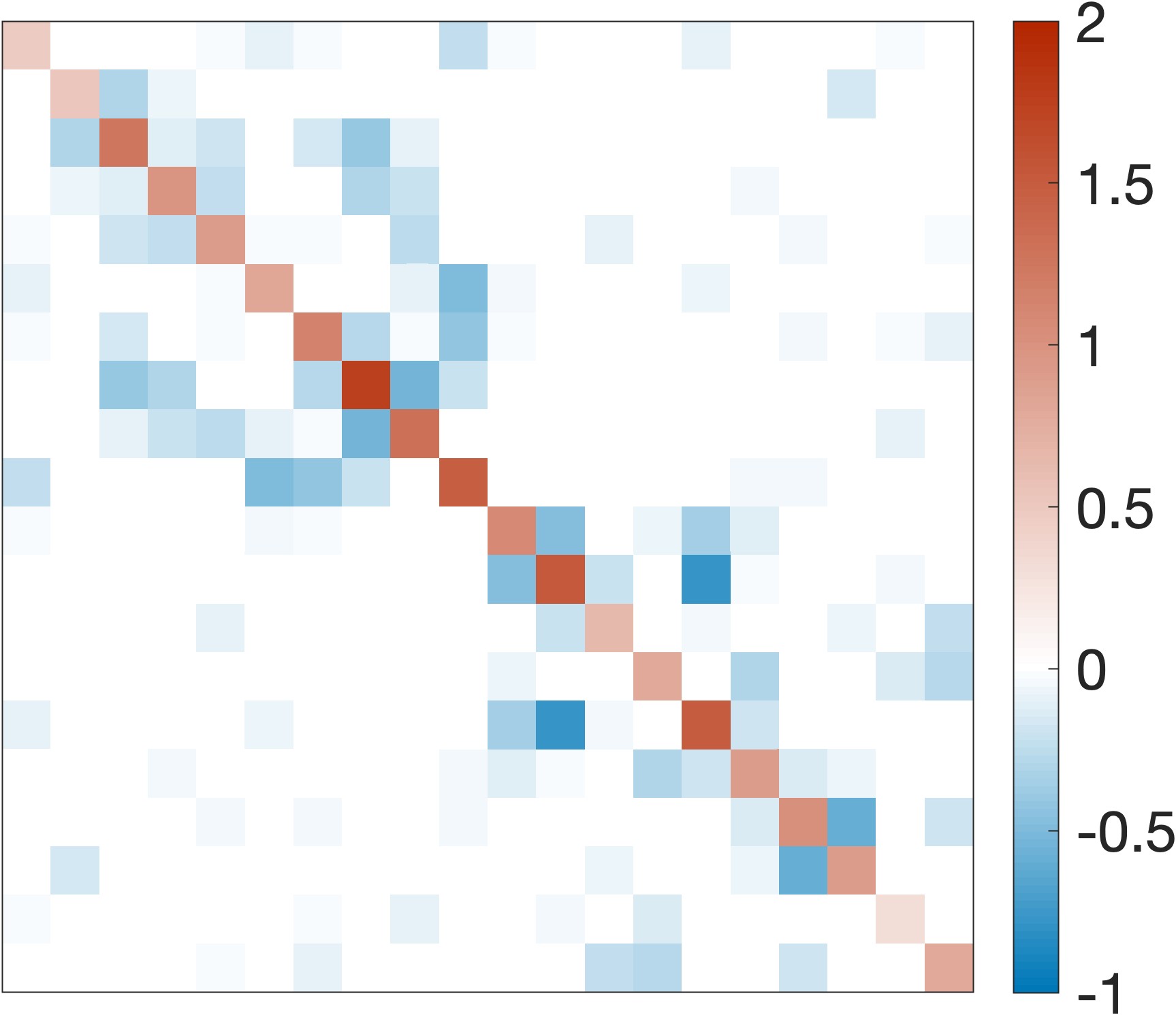
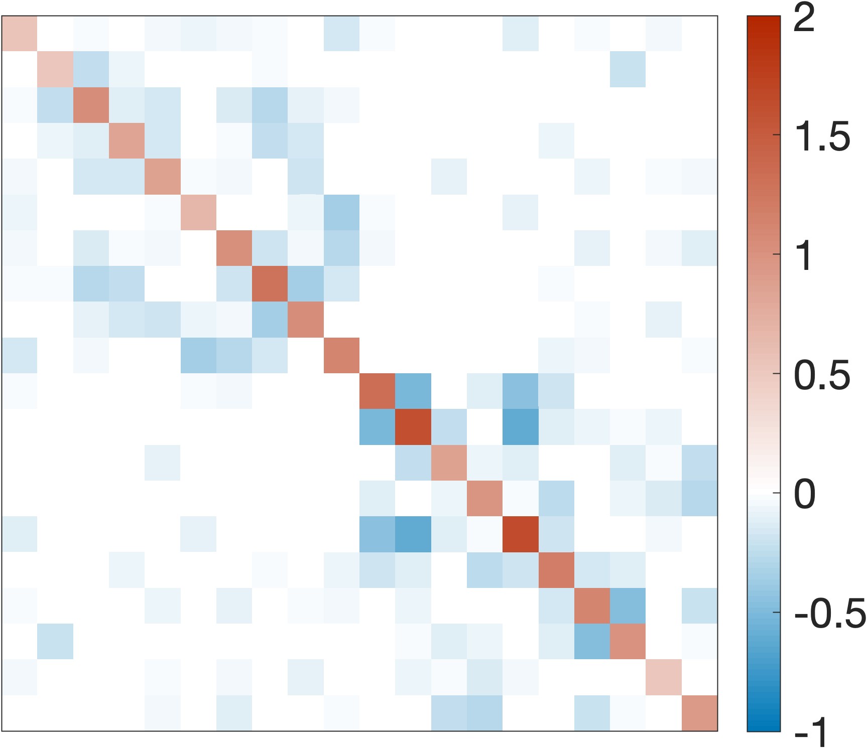
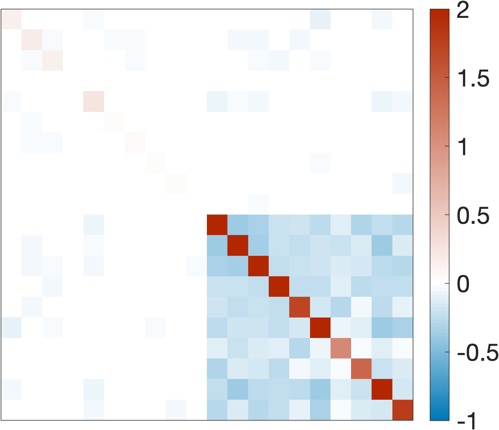
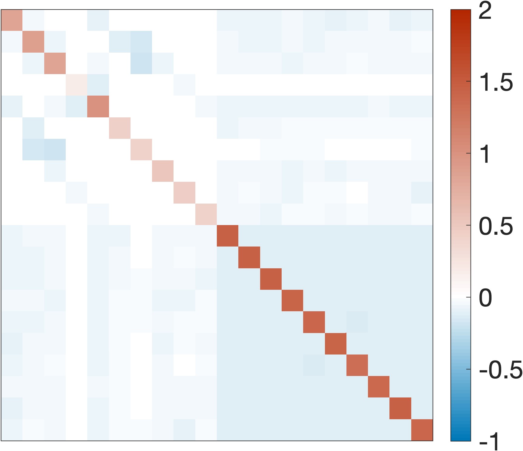
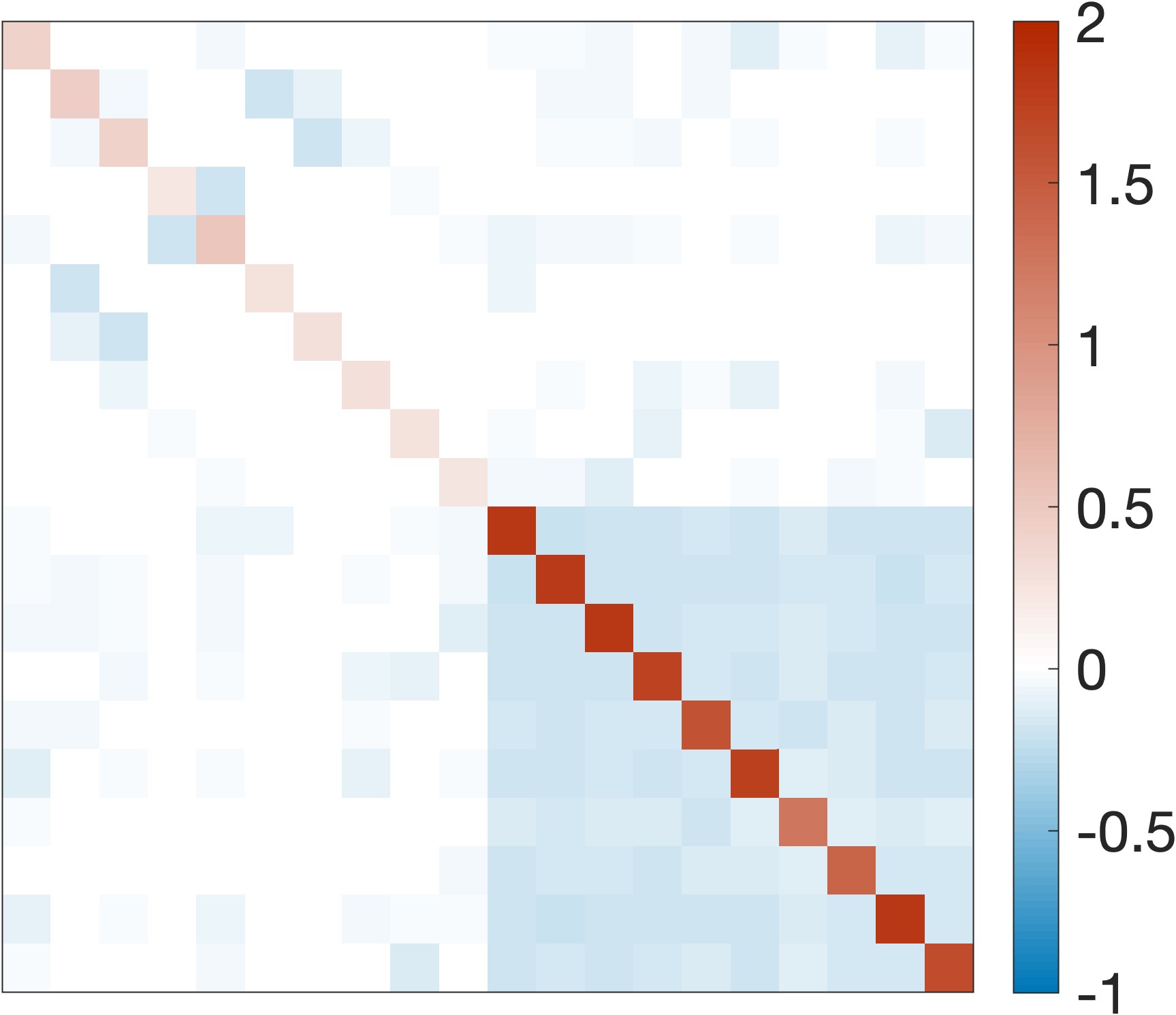
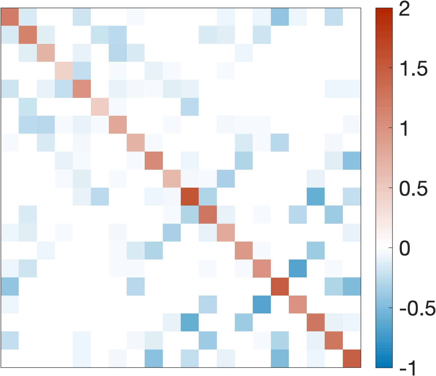
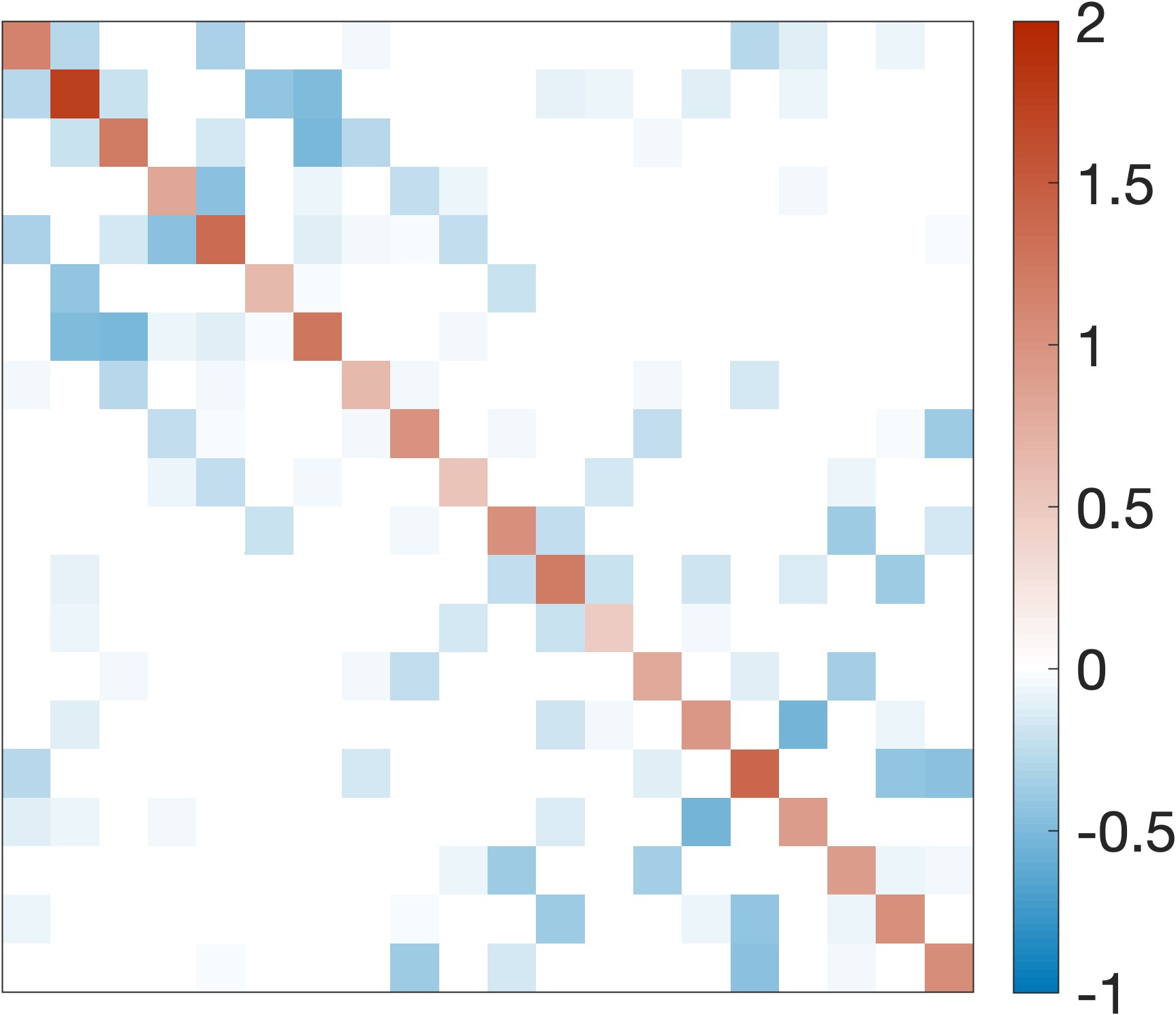
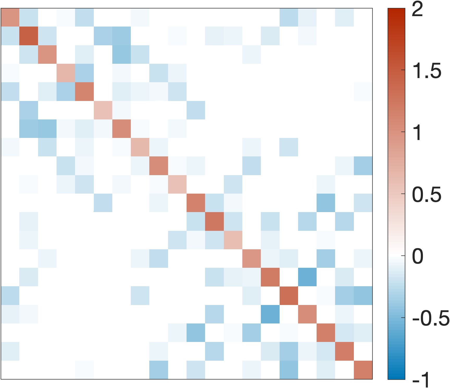
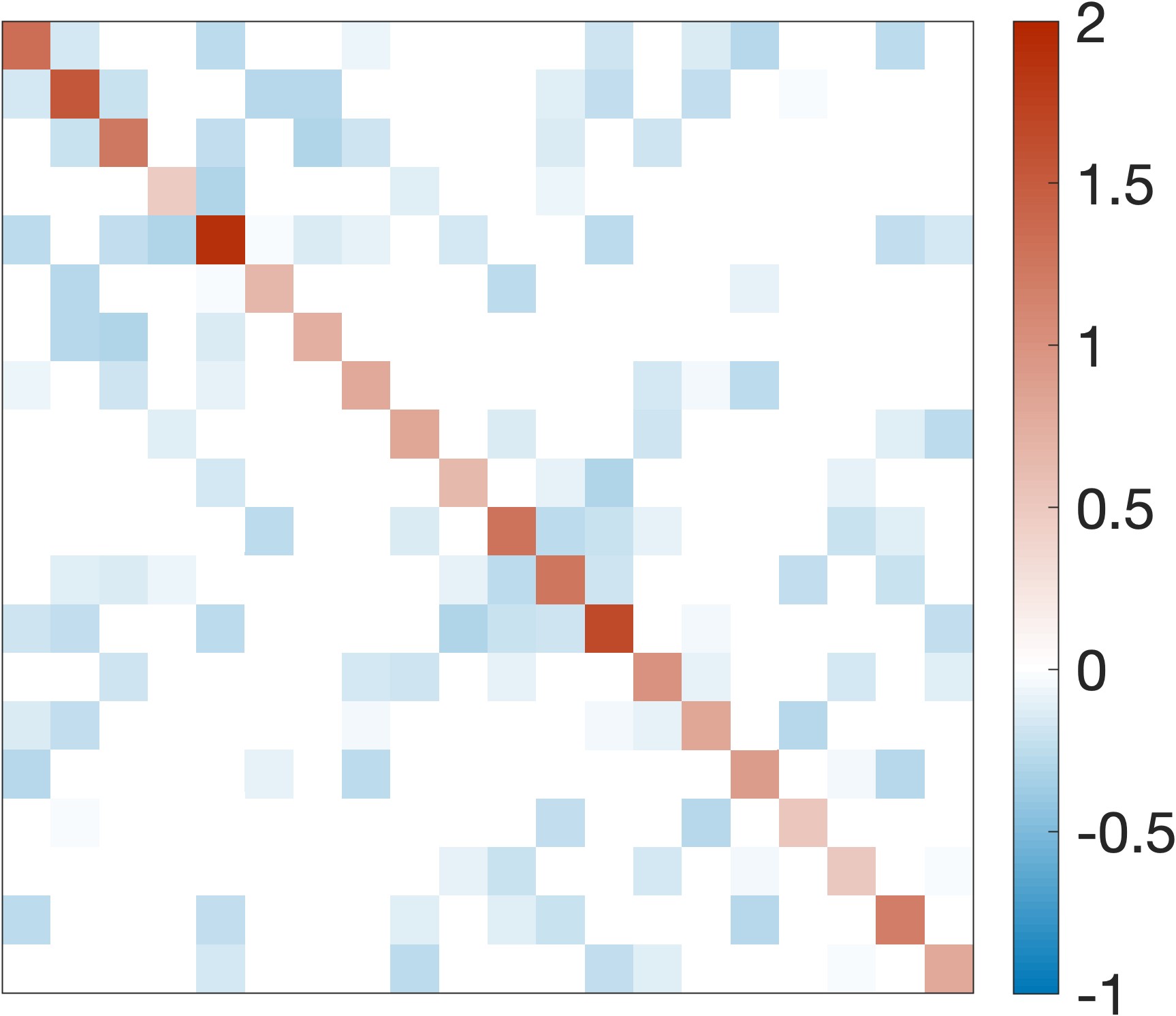
Figure 5: Graph Laplacians estimated by different methods and the ground truth Erdős-Rényi graph Laplacian (p=0.3).

SCGL	GLS-1	GLS-2	CGL	GLEN	GLEN-VI	Ground Truth

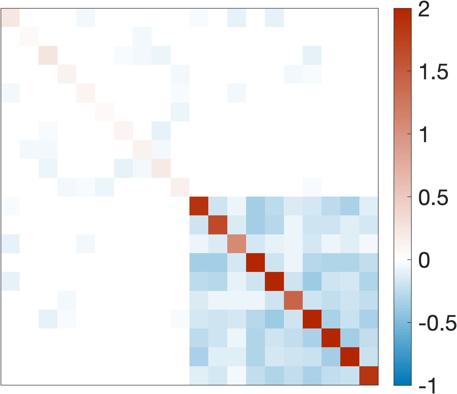
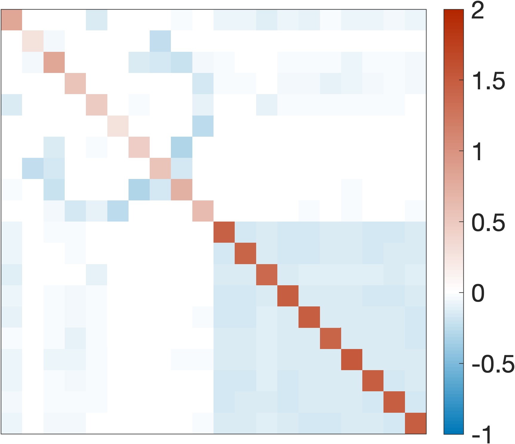
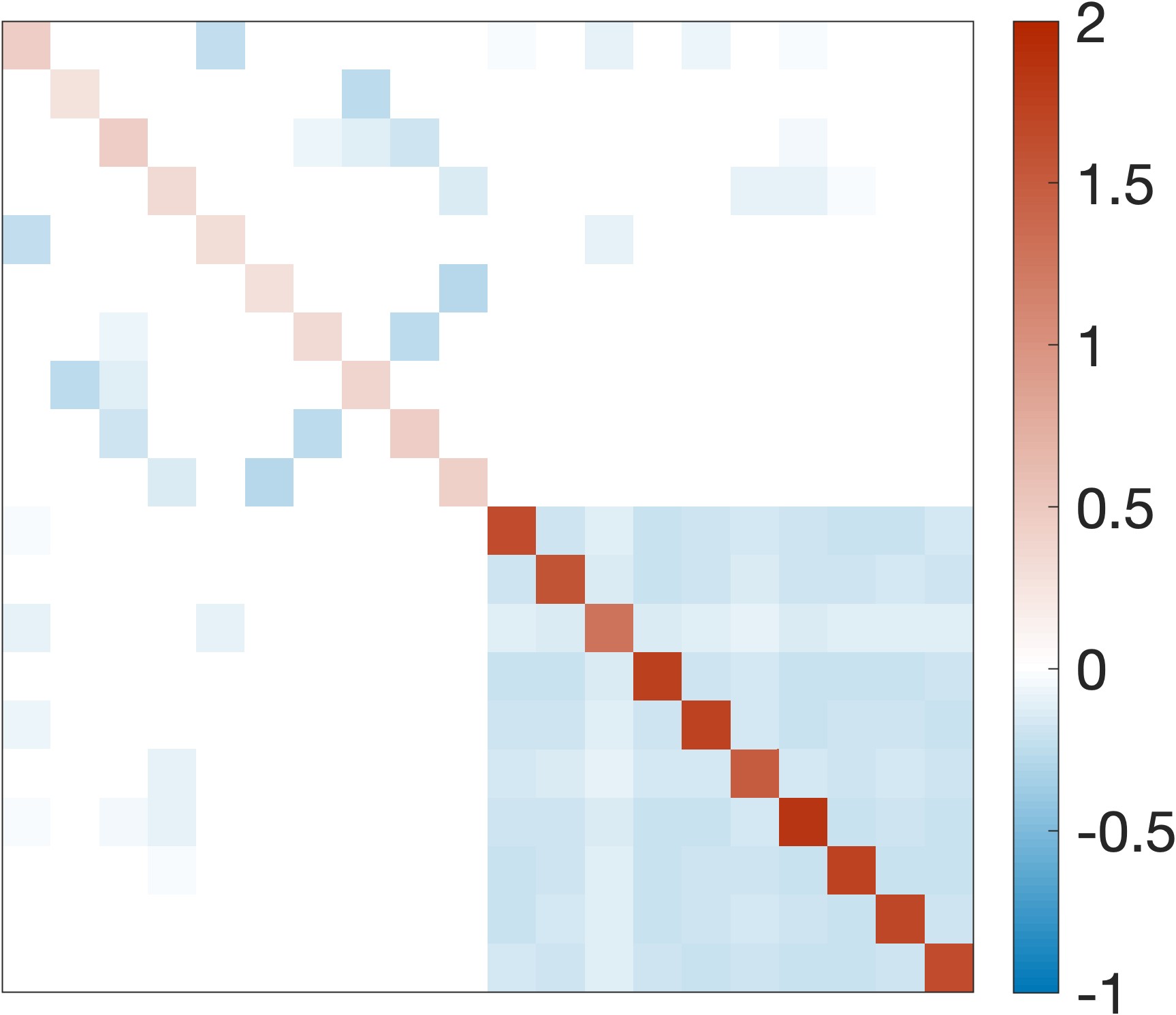
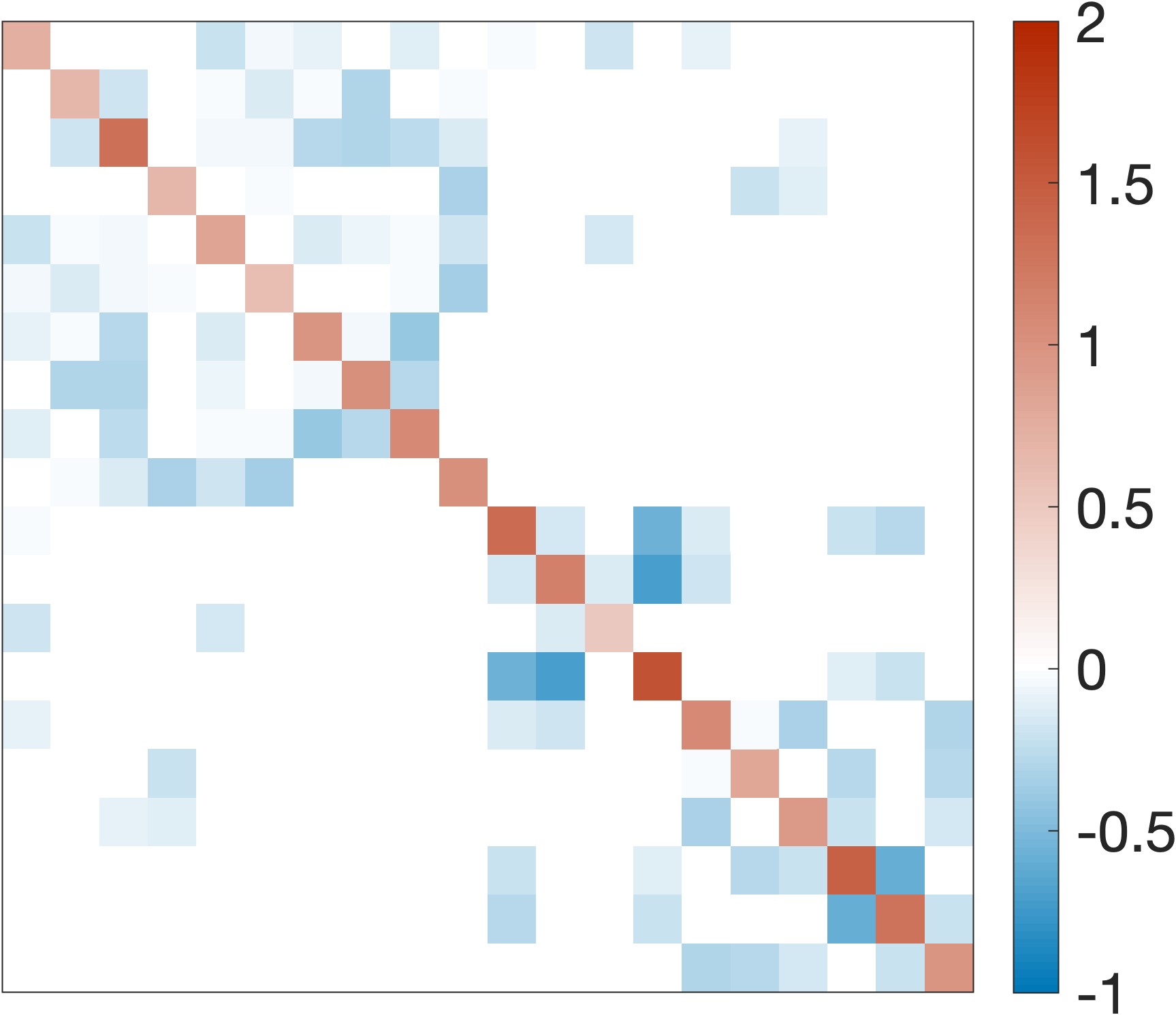
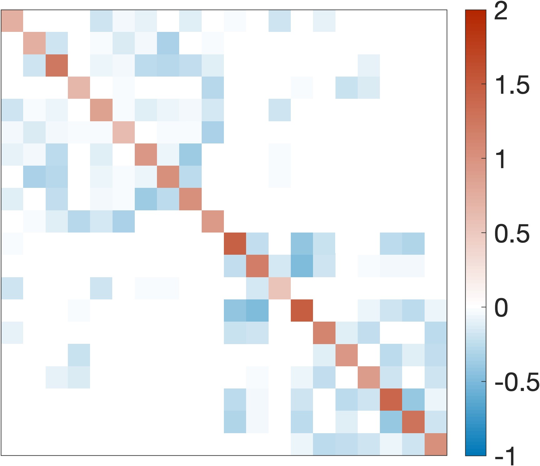
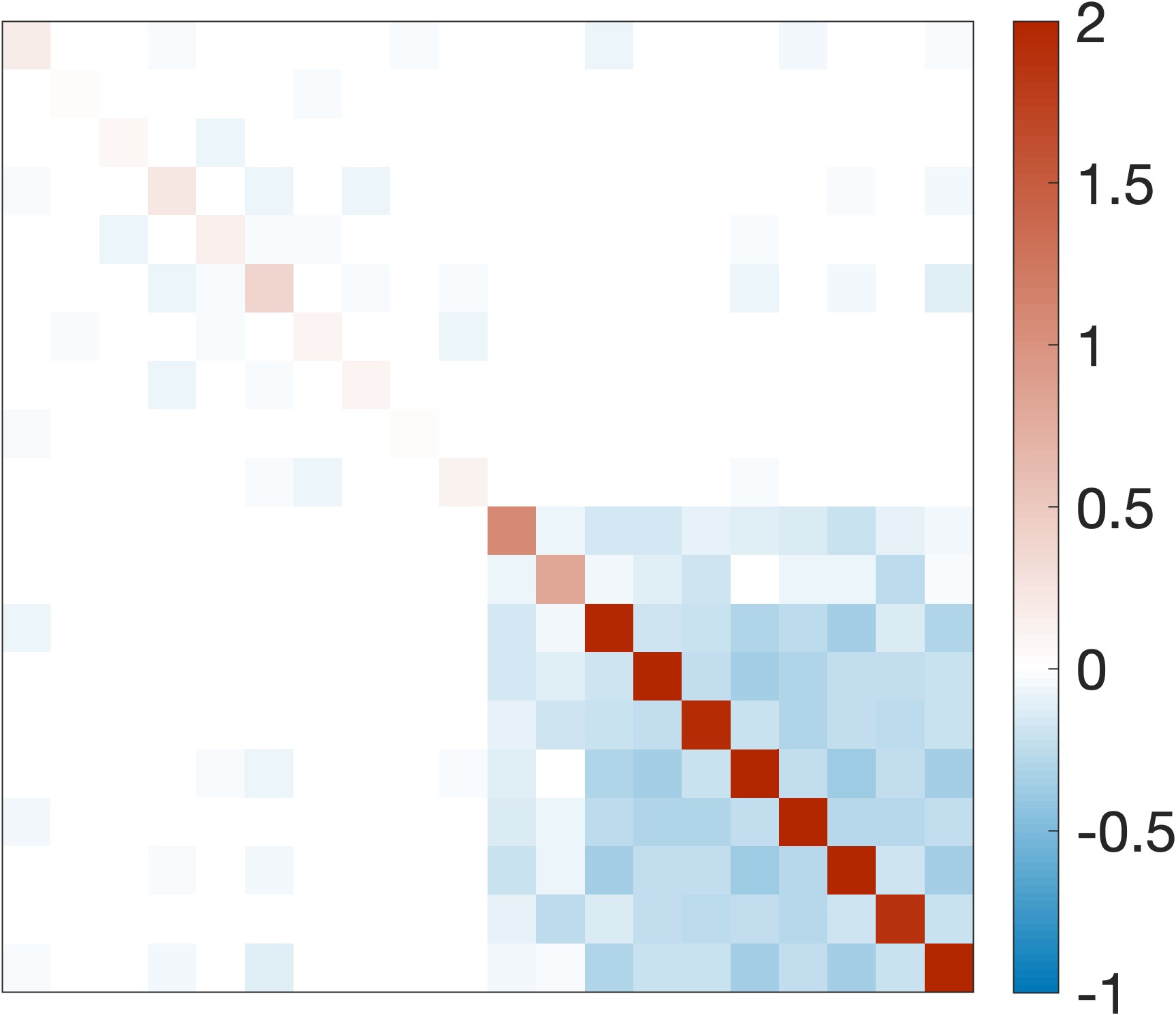
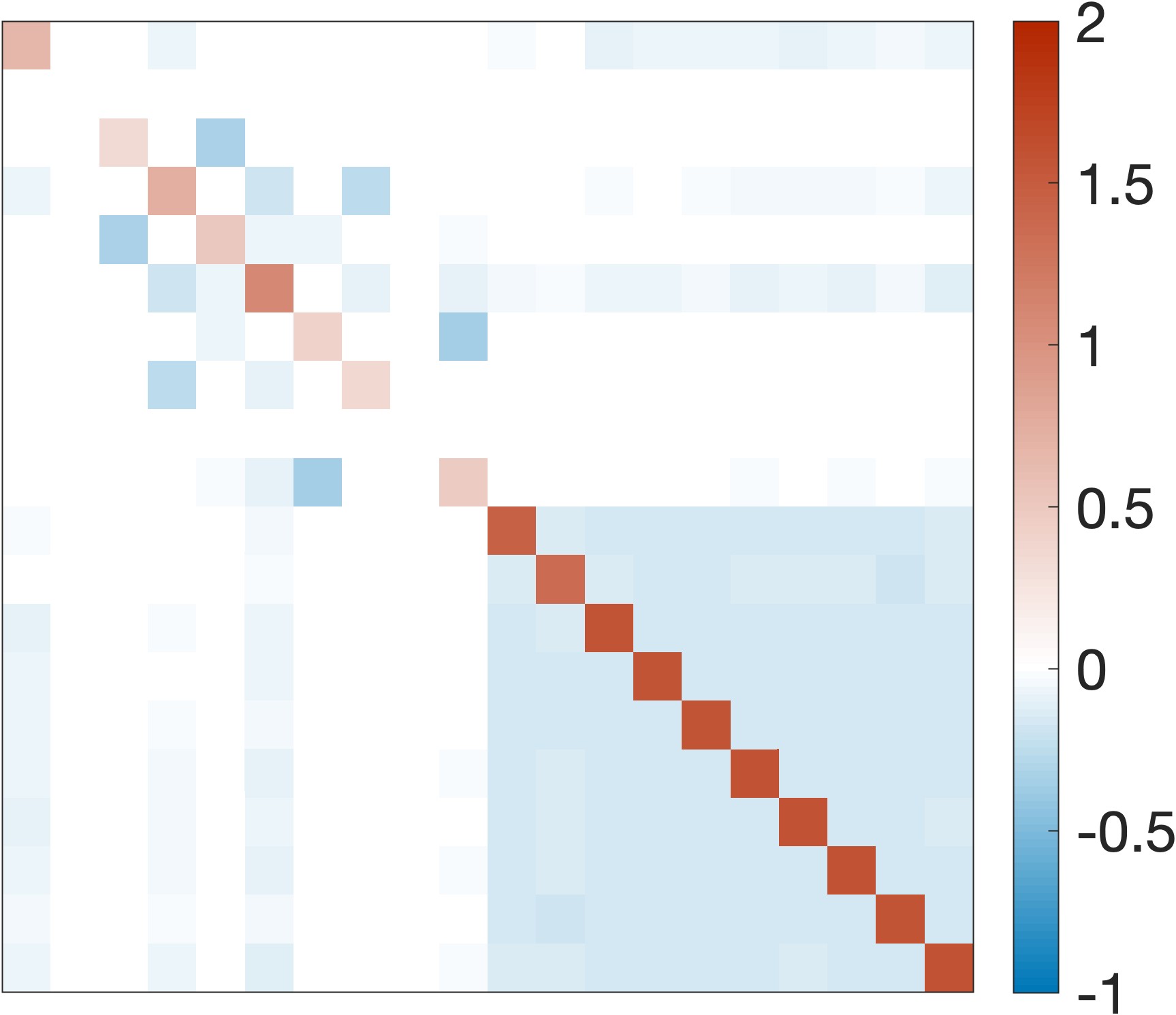
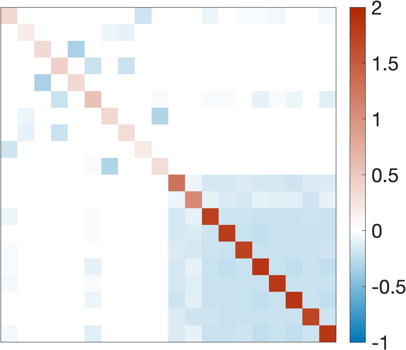
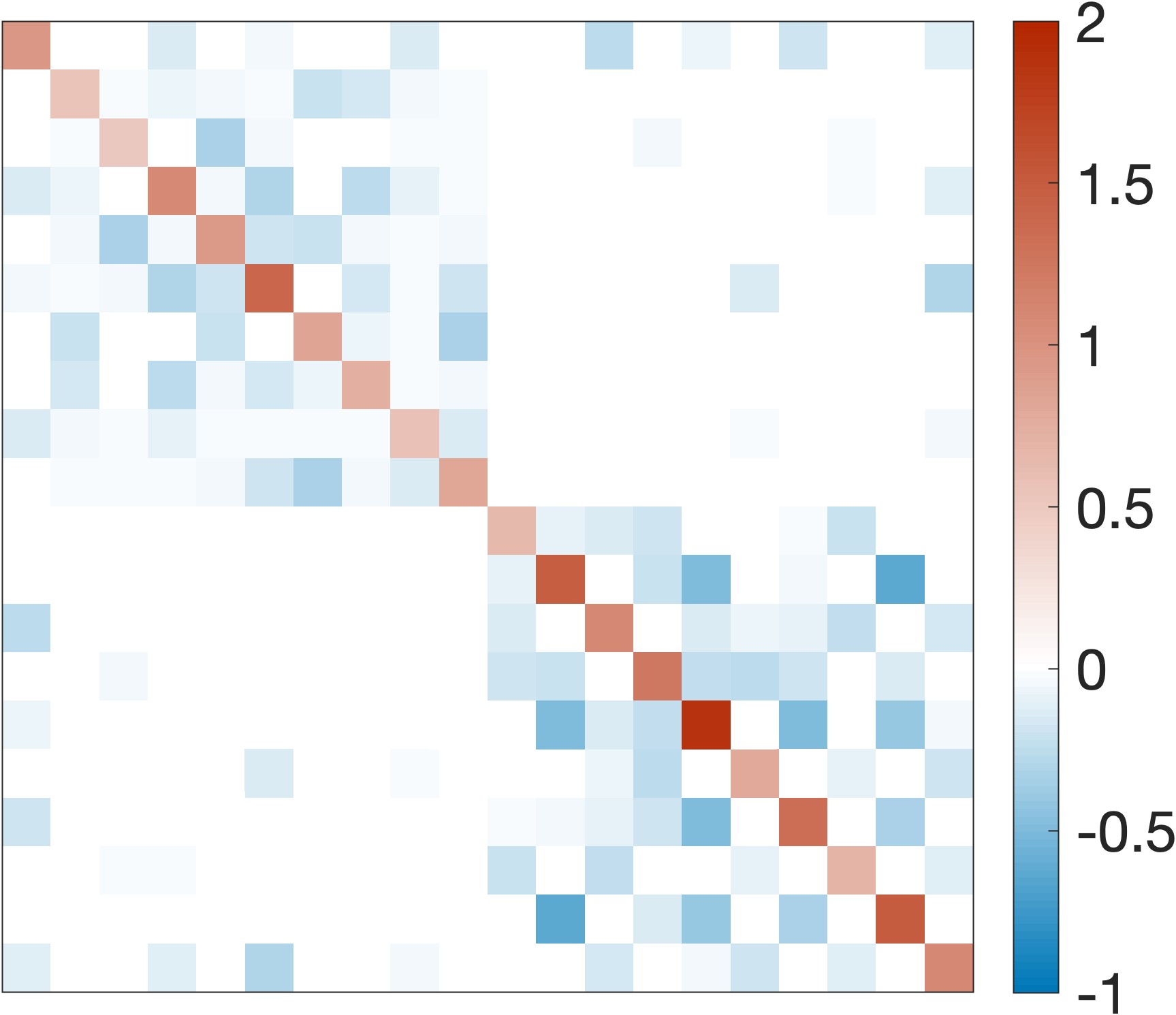
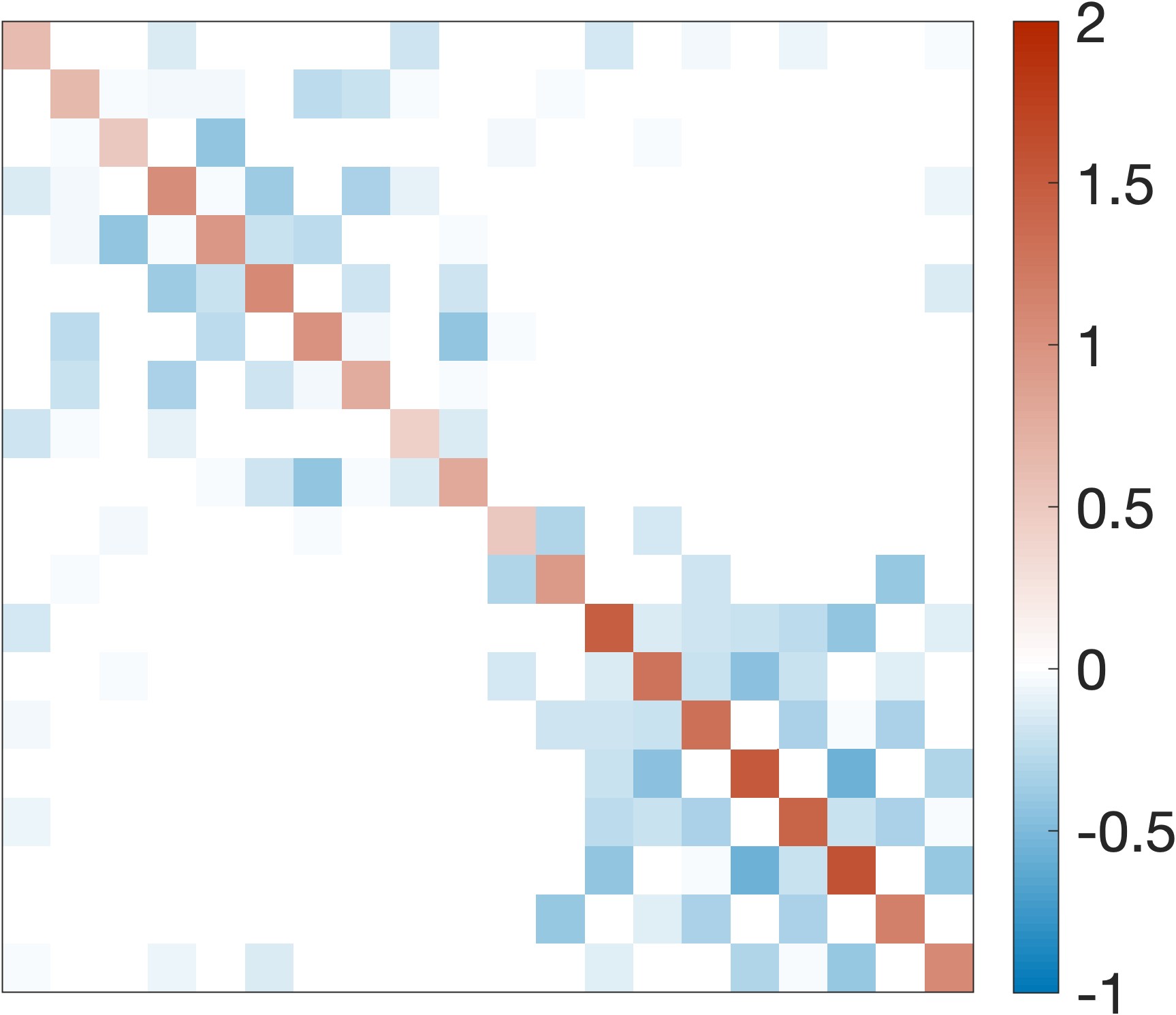
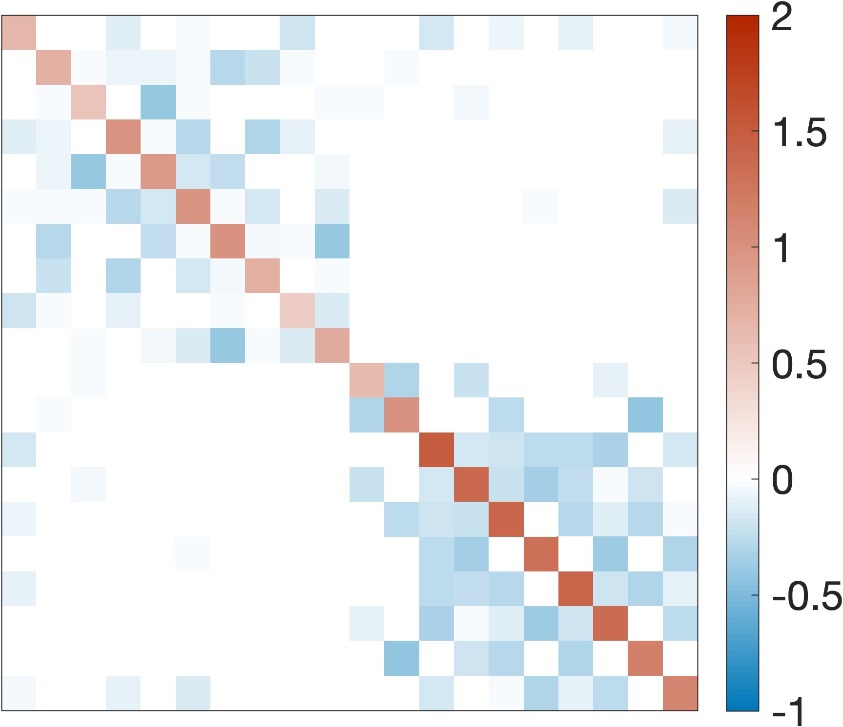
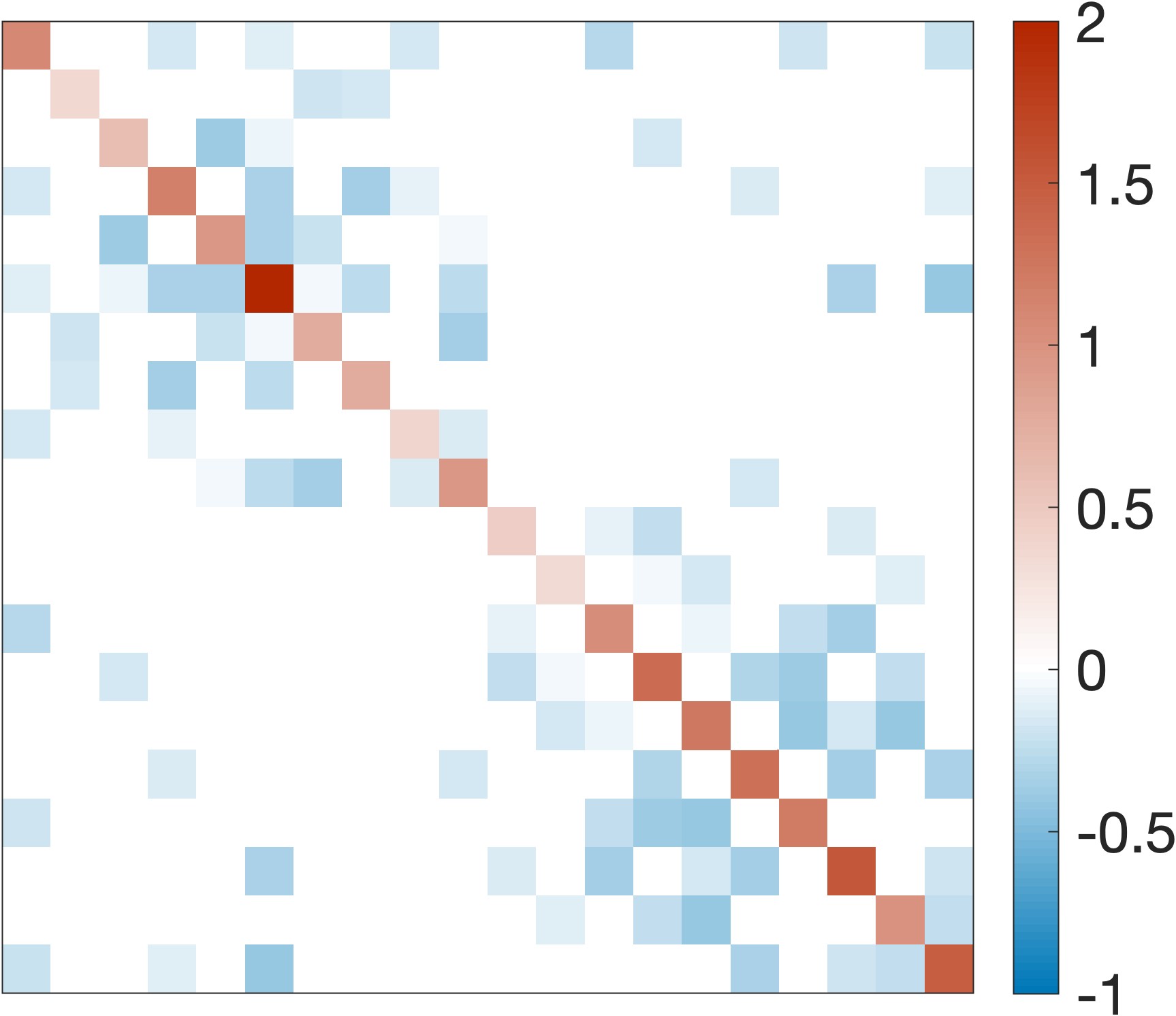
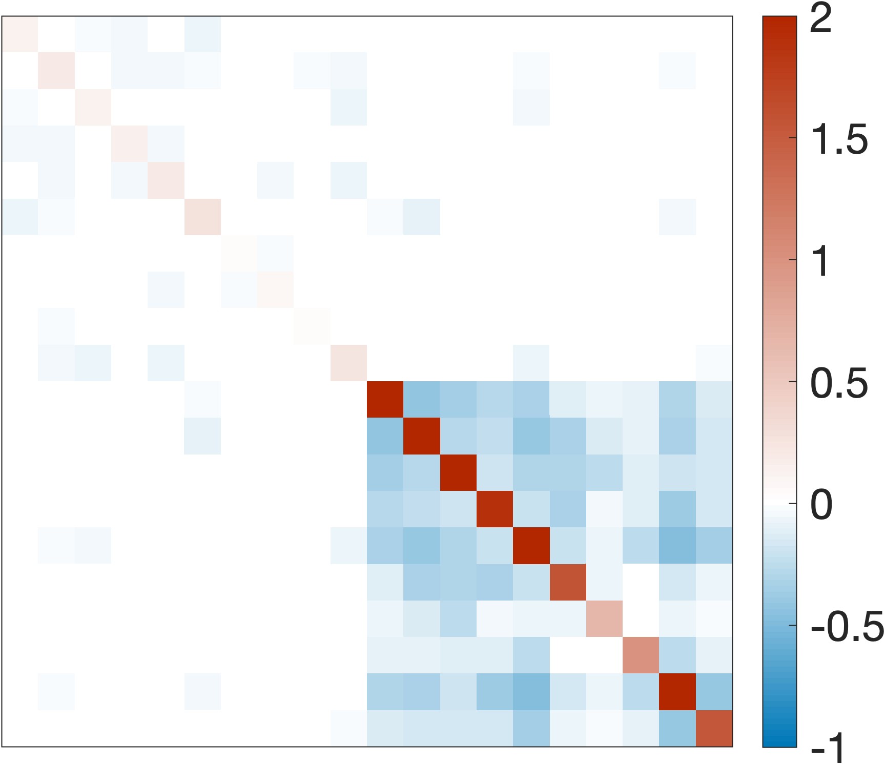
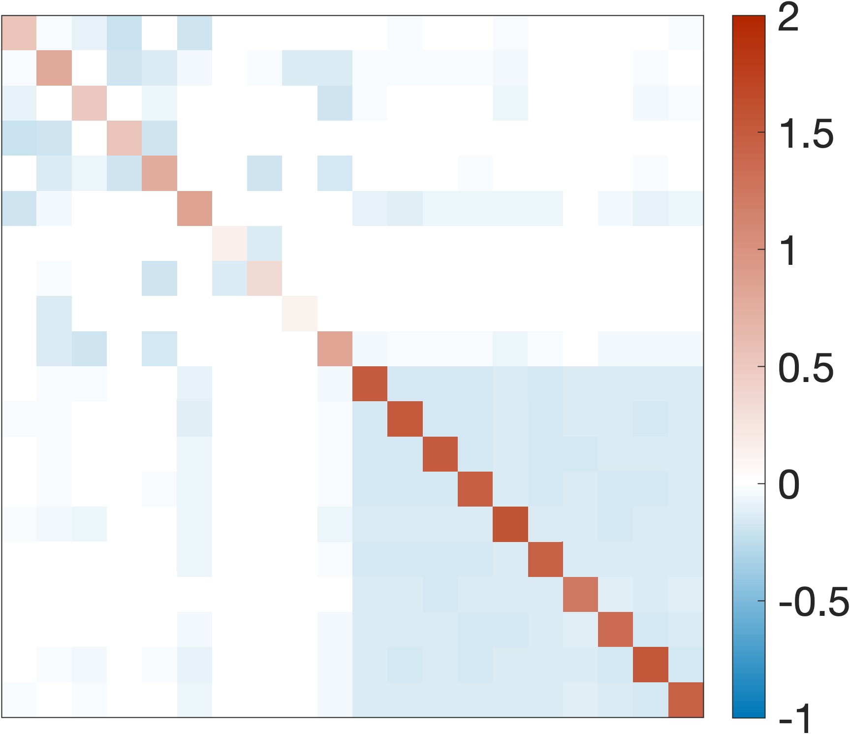
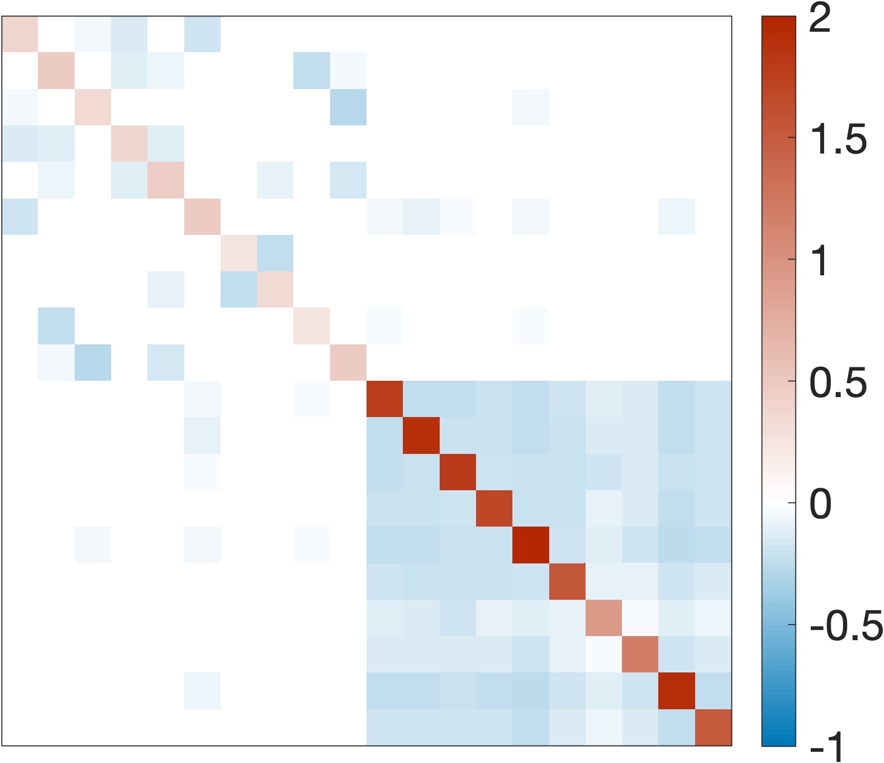
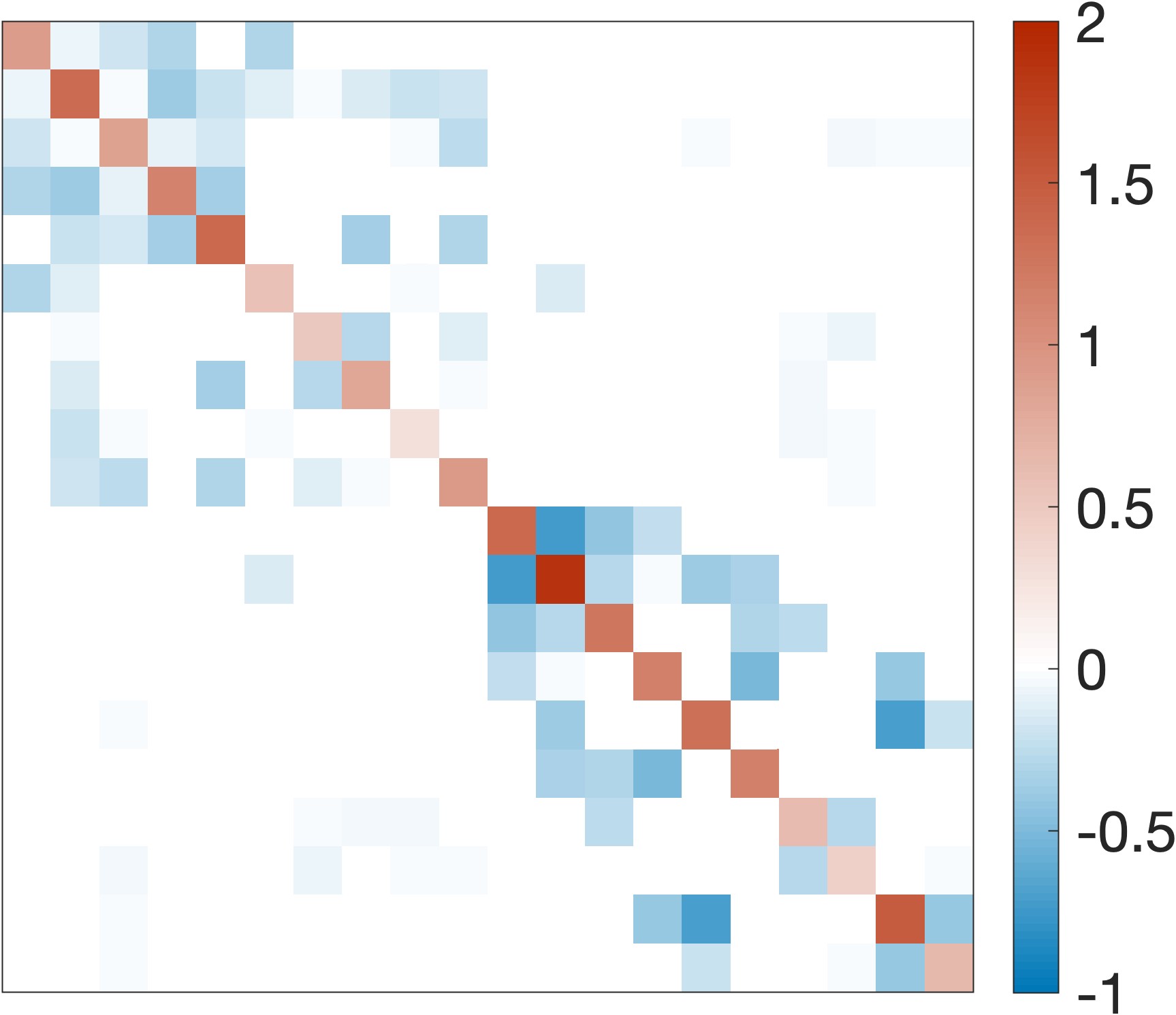
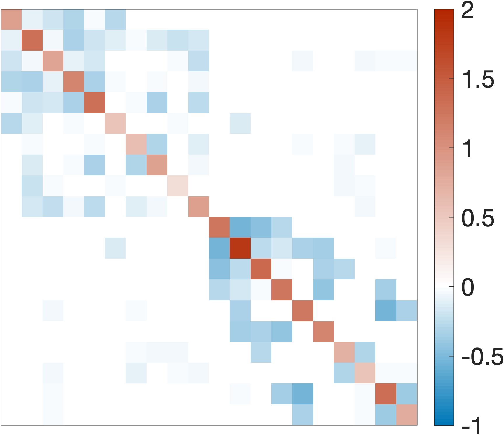
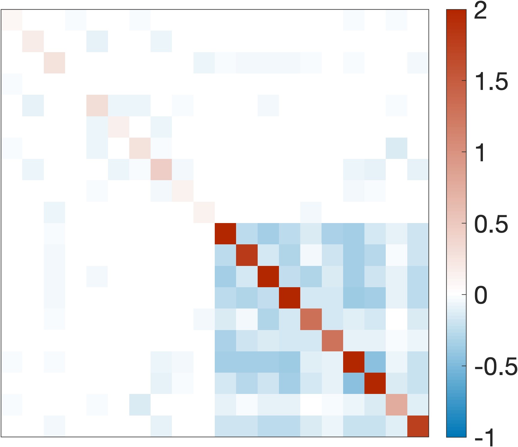
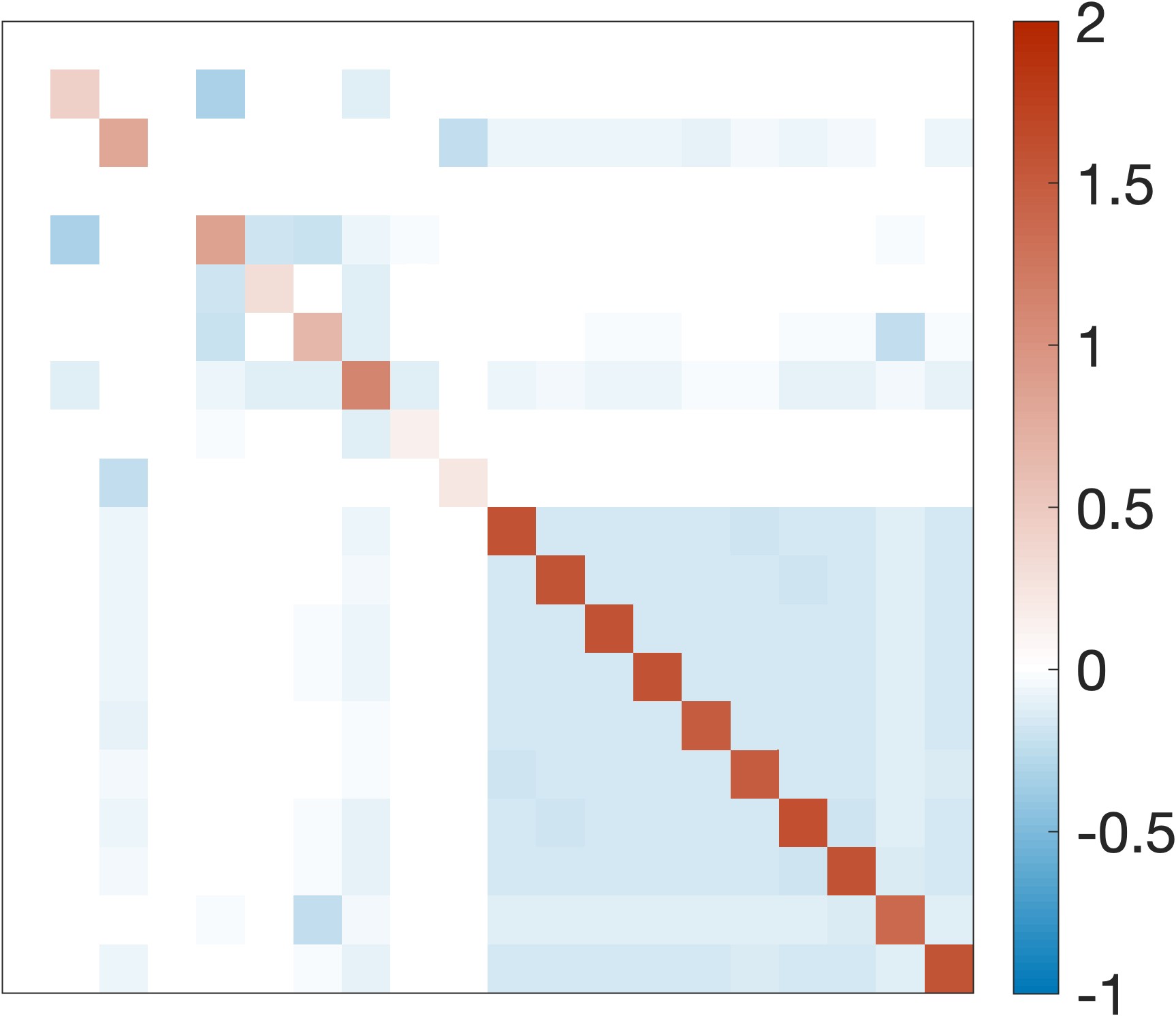
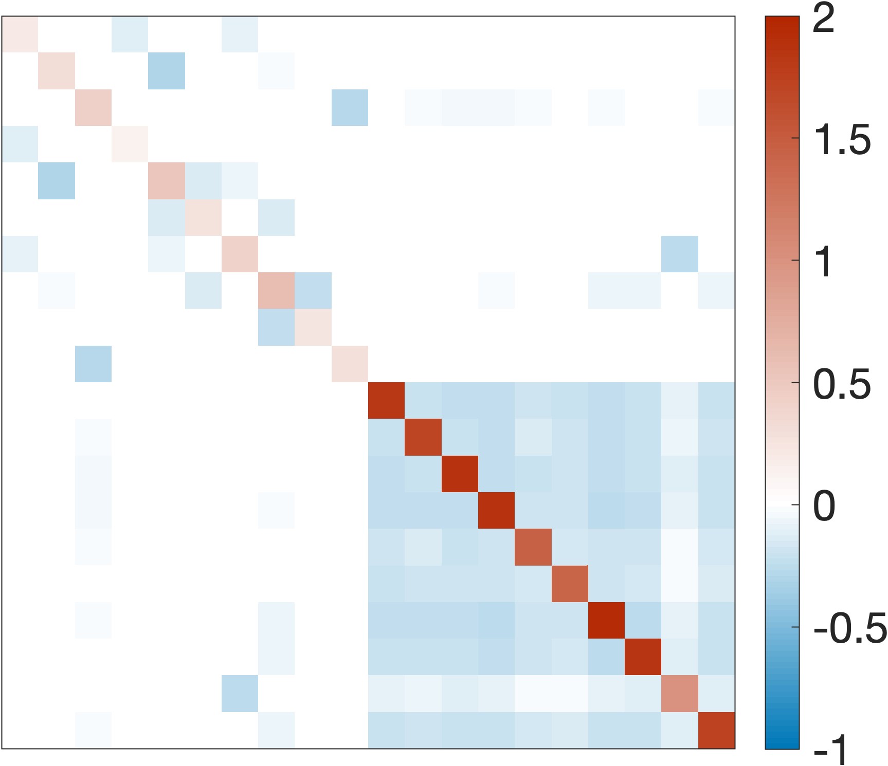
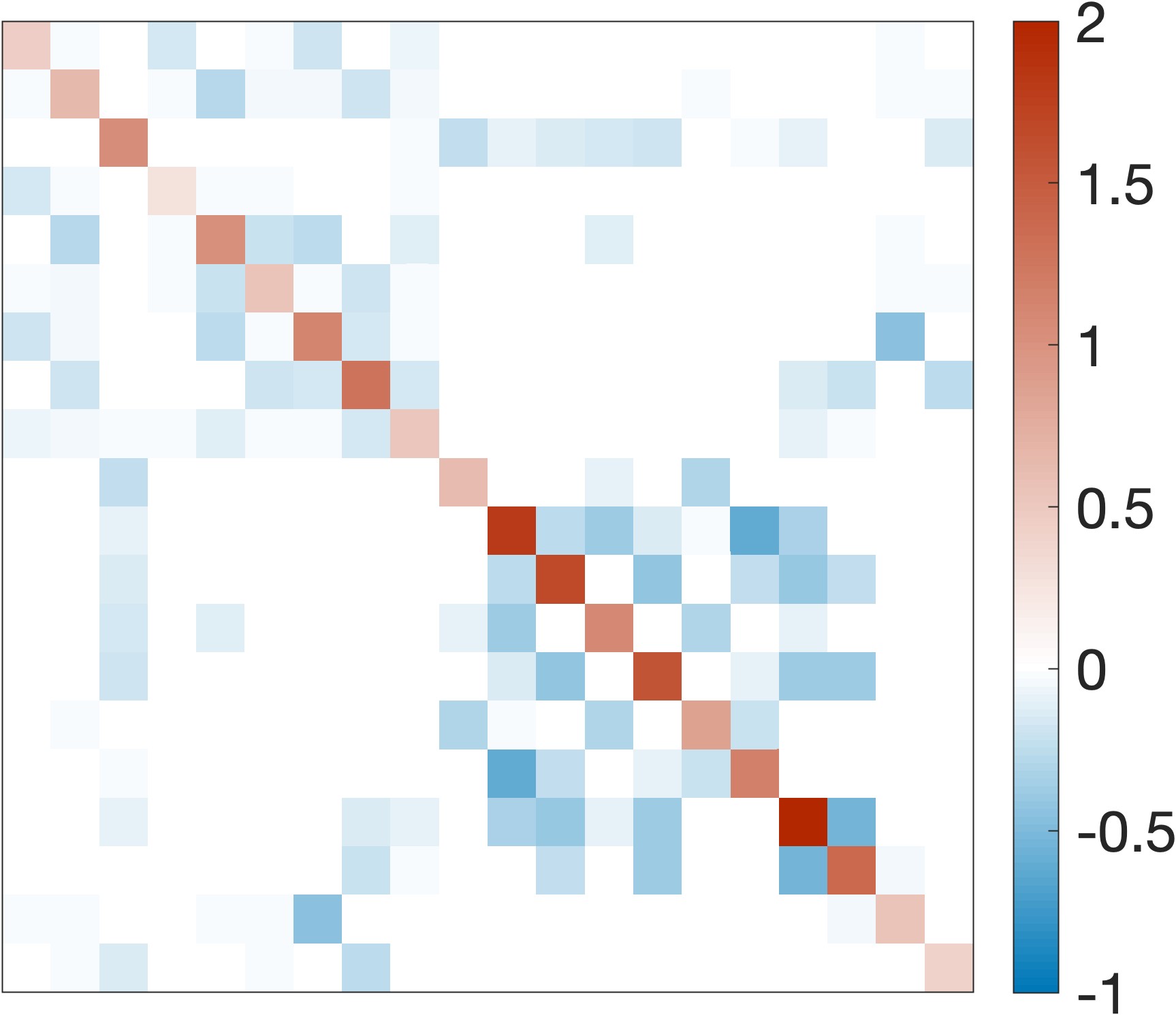
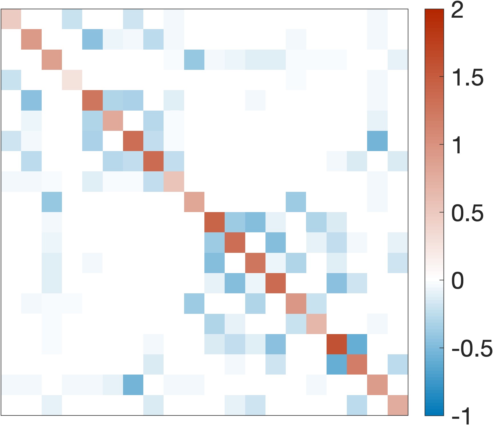
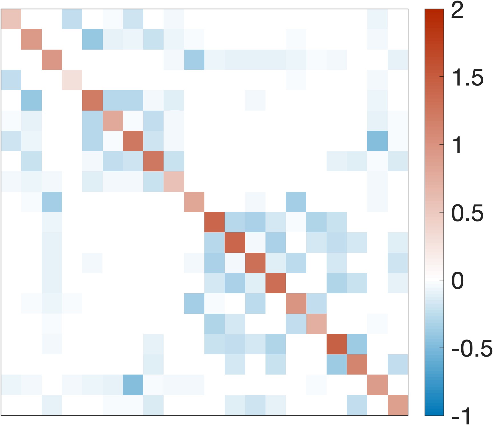
Figure 6: Graph Laplacians estimated by different methods and the ground truth stochastic block graph Laplacian (p=0.4,q=0.1).

SCGL	GLS-1	GLS-2	CGL	GLEN	GLEN-VI	Ground Truth

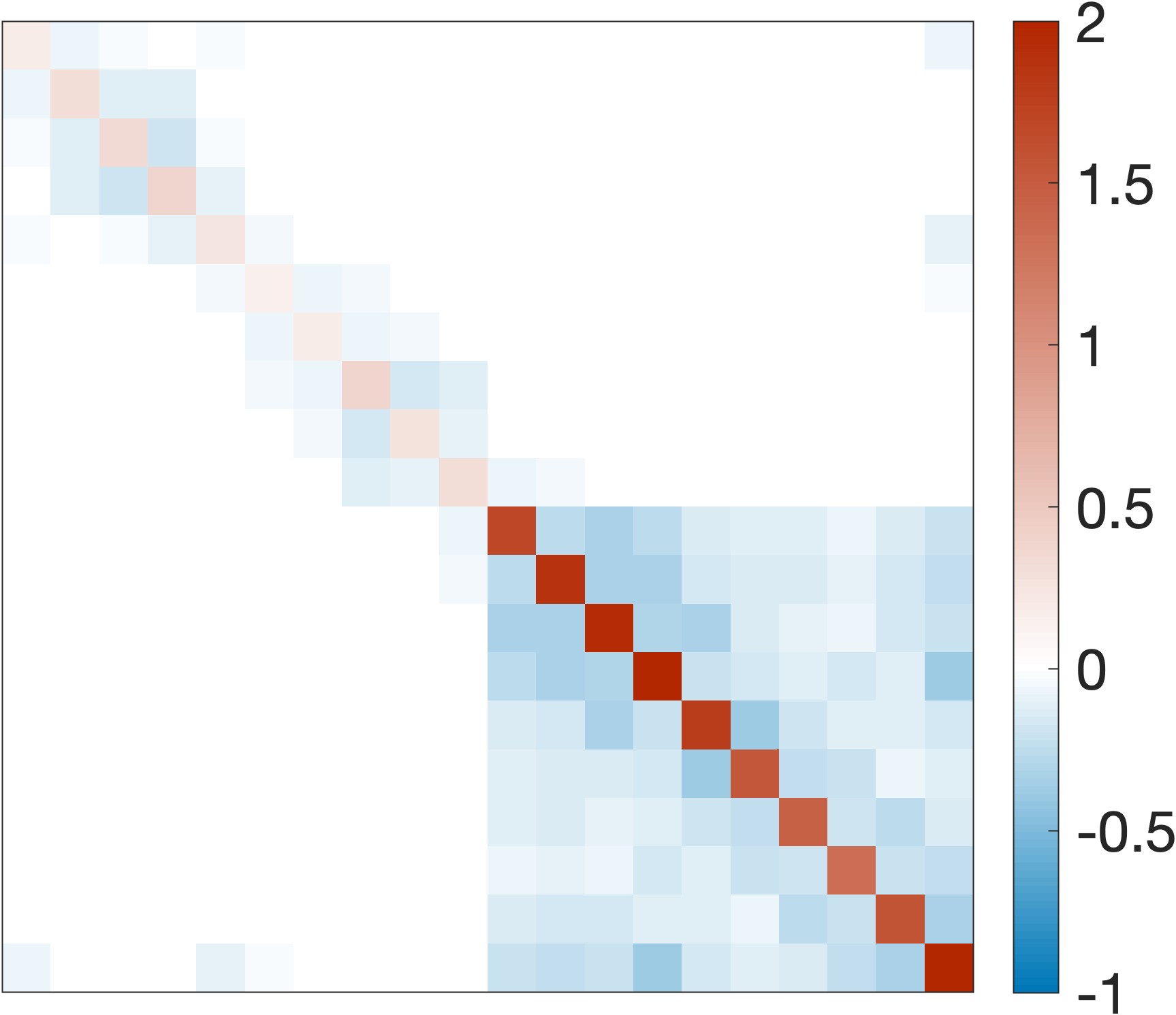
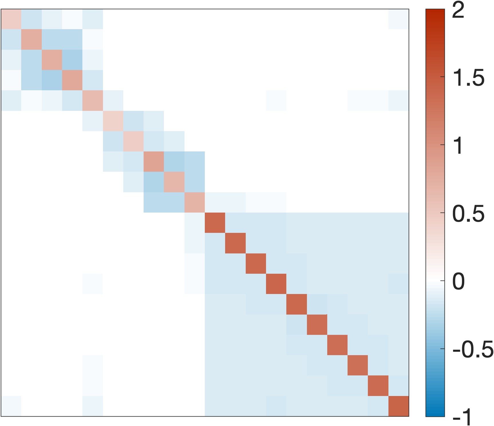
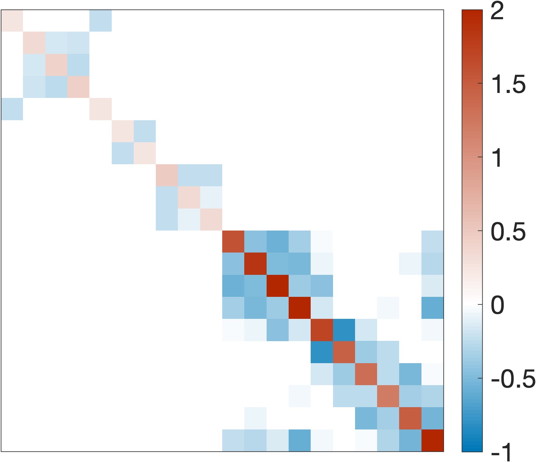
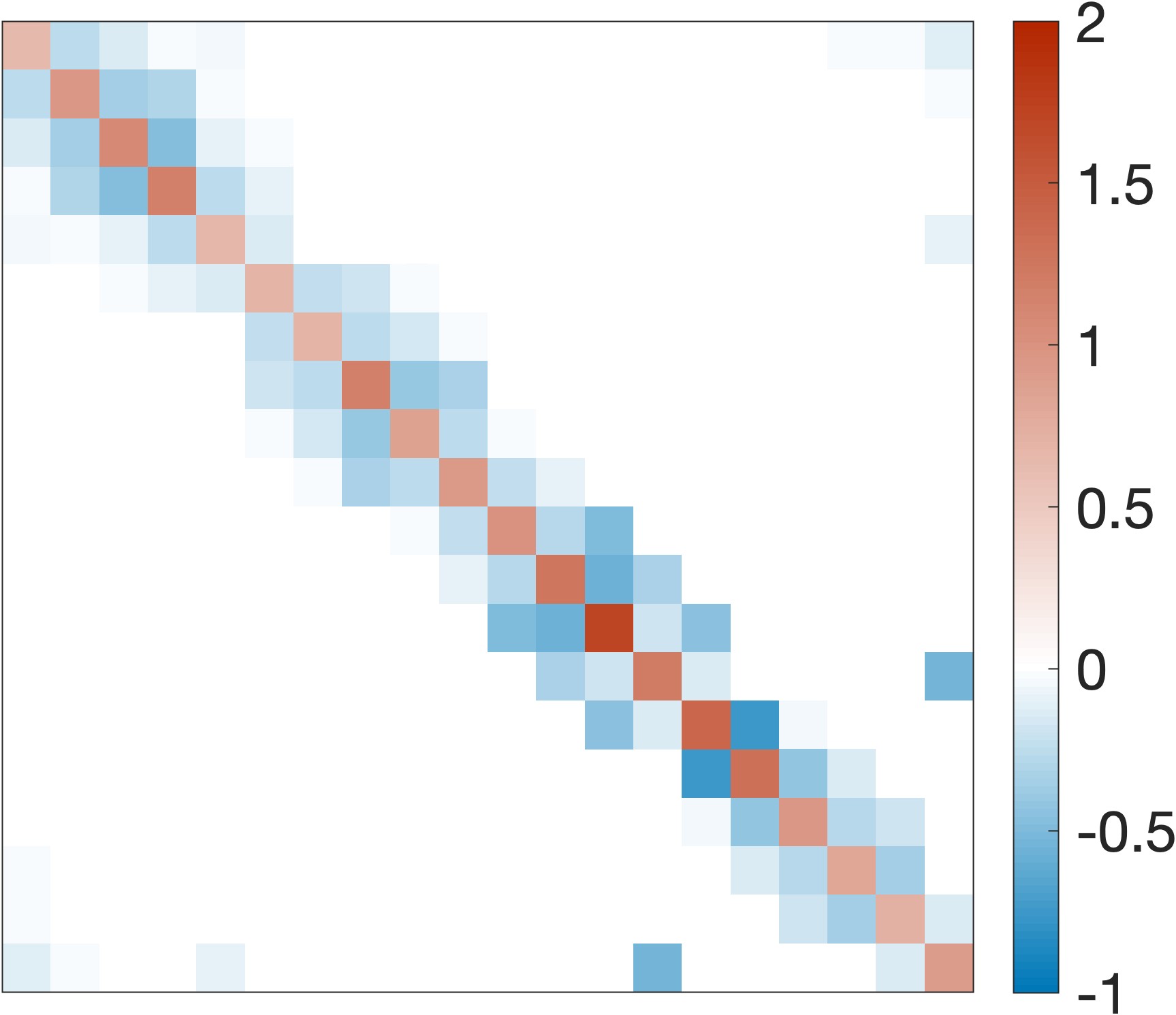
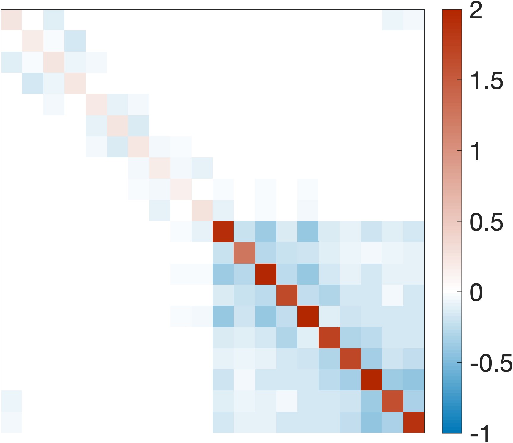
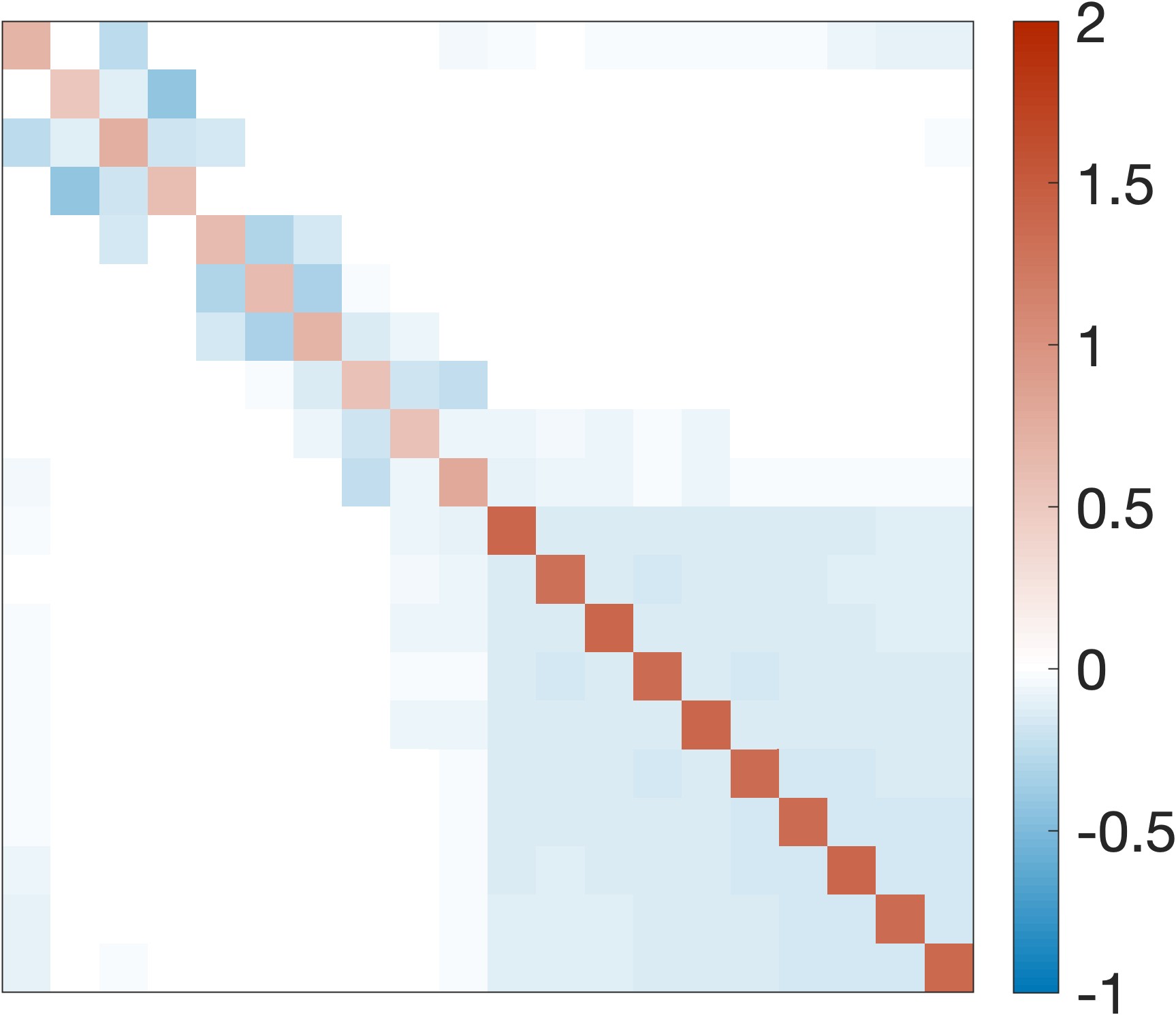
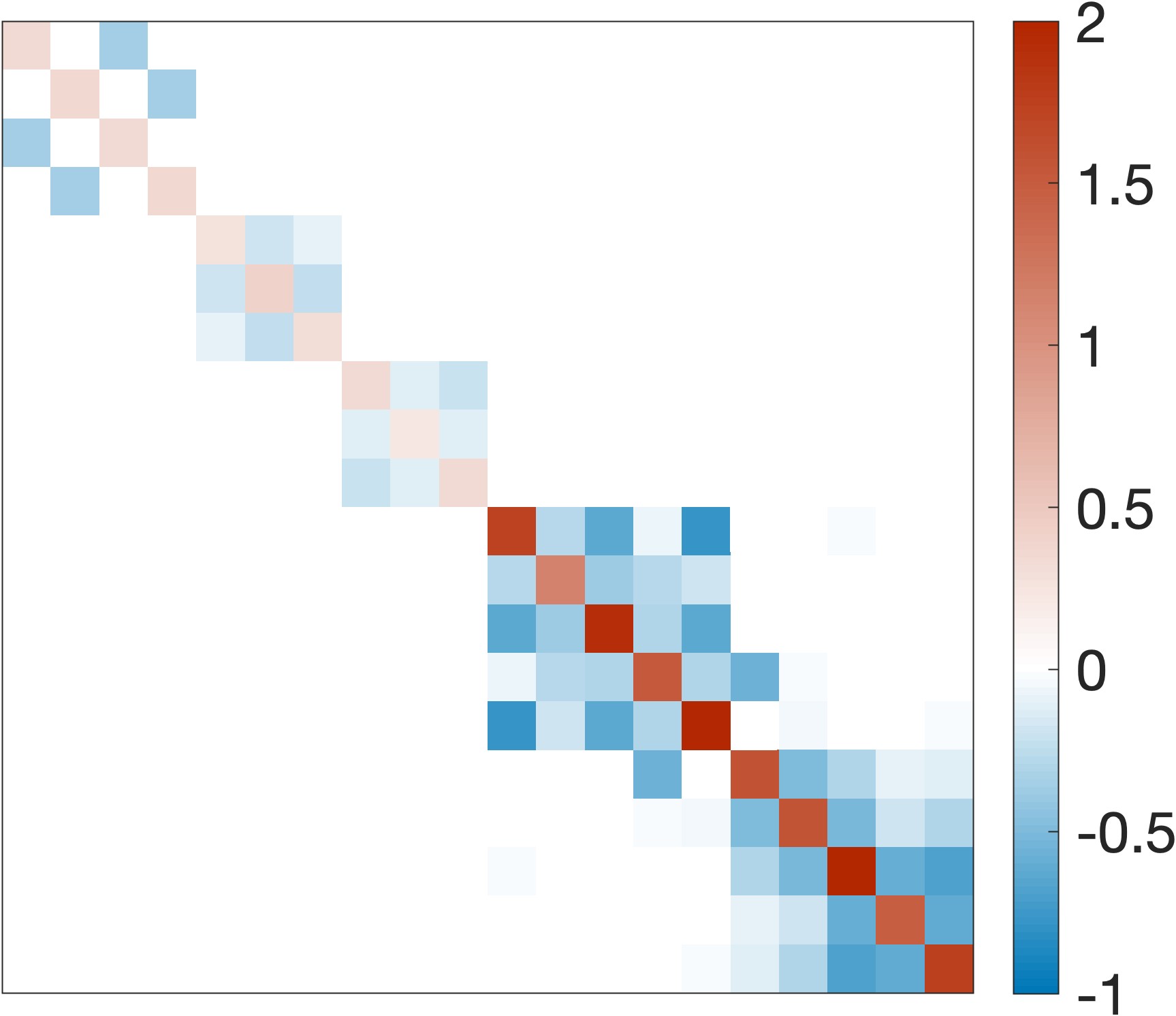
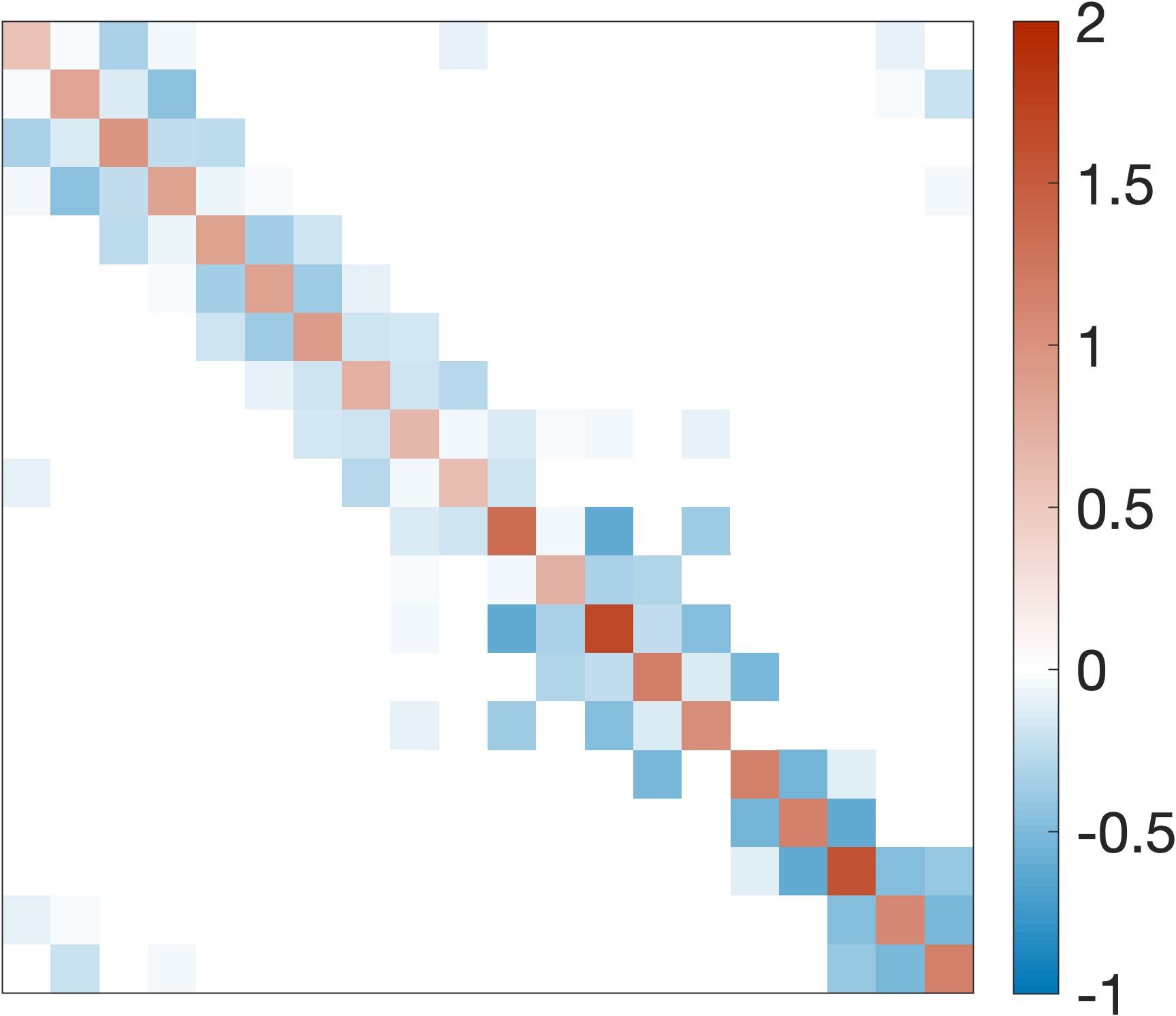
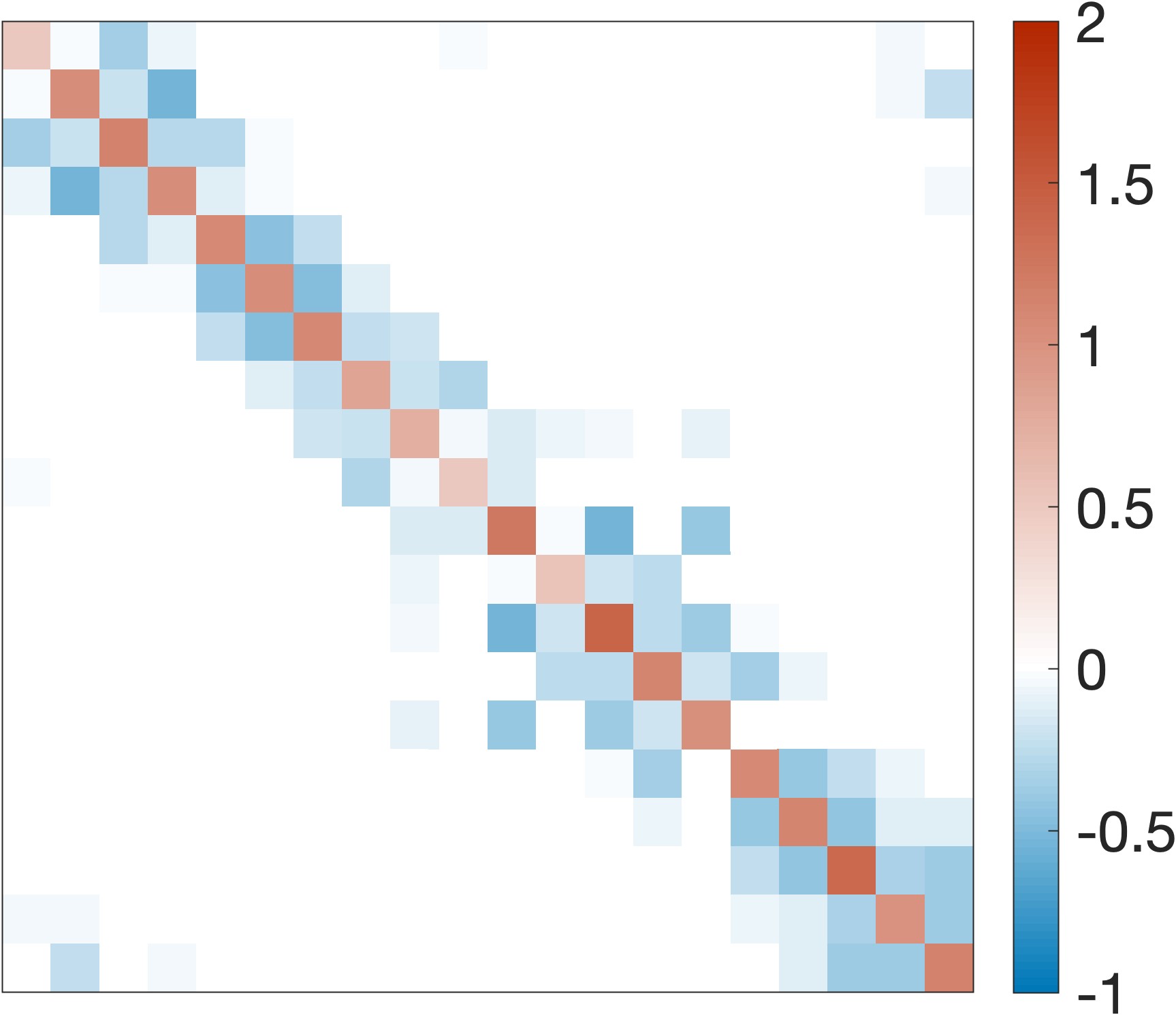
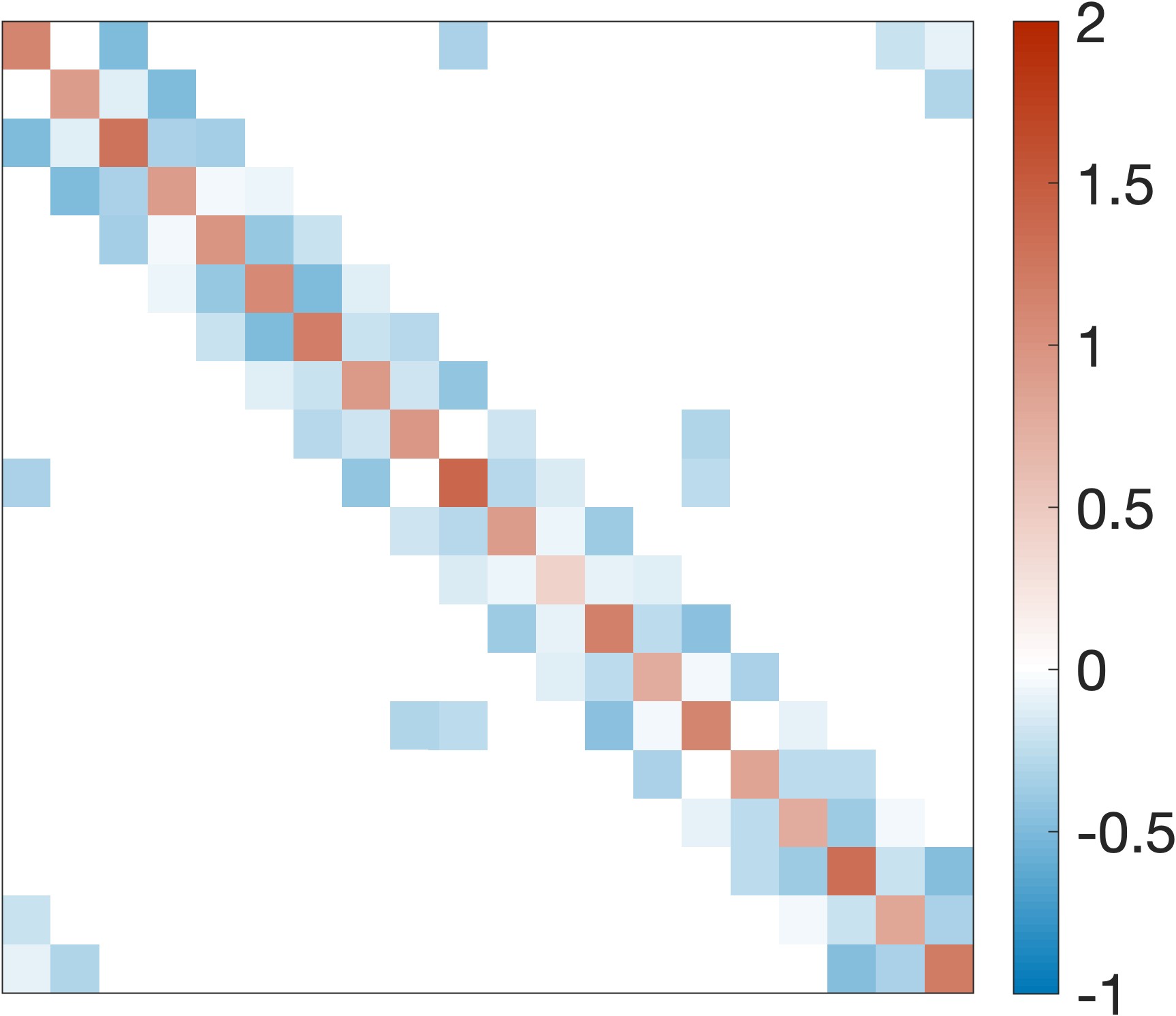
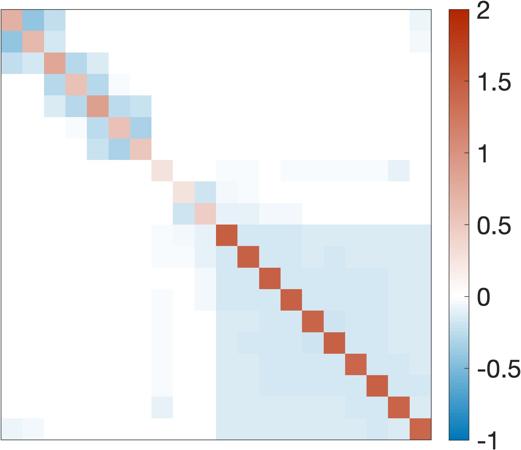
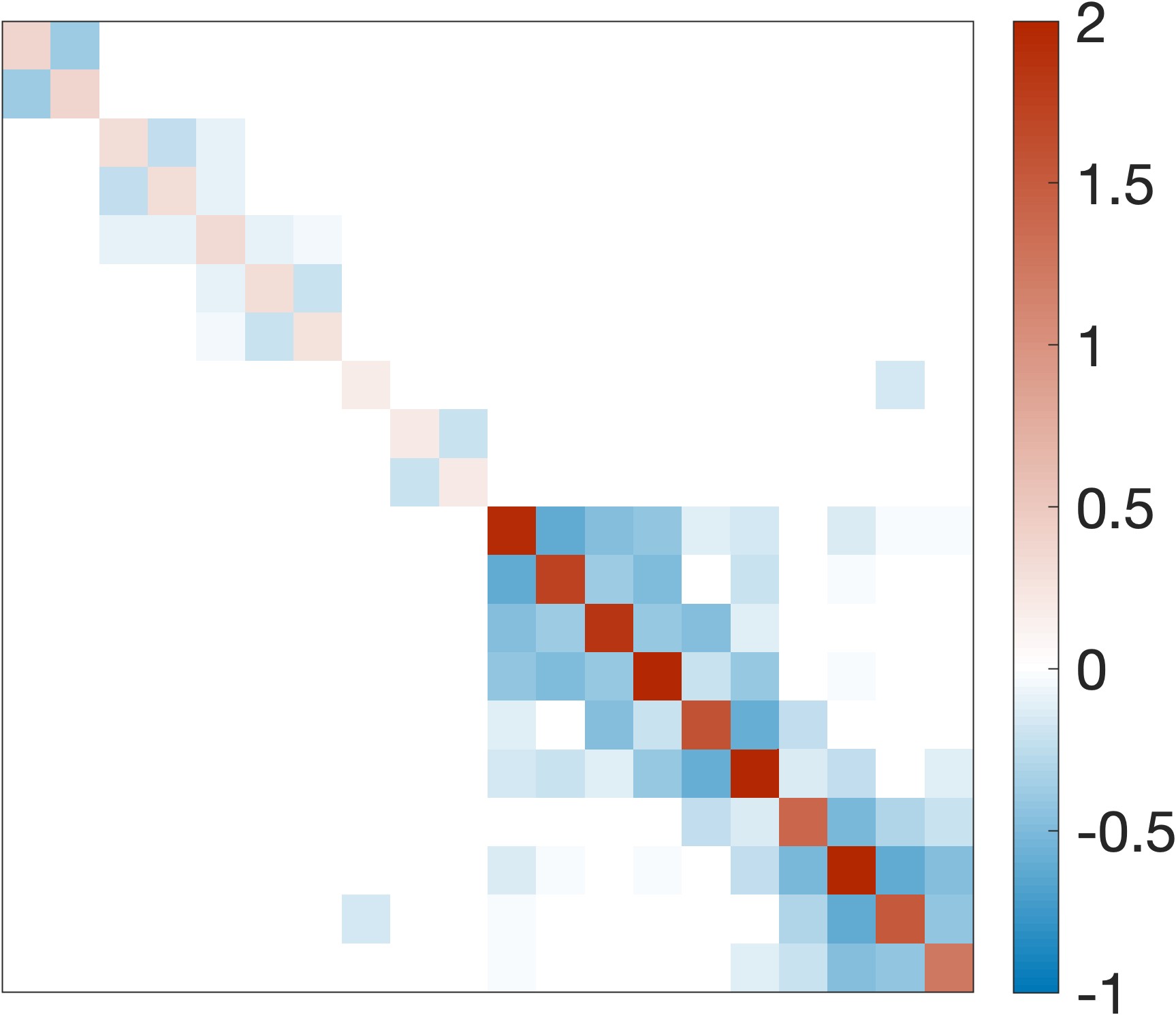
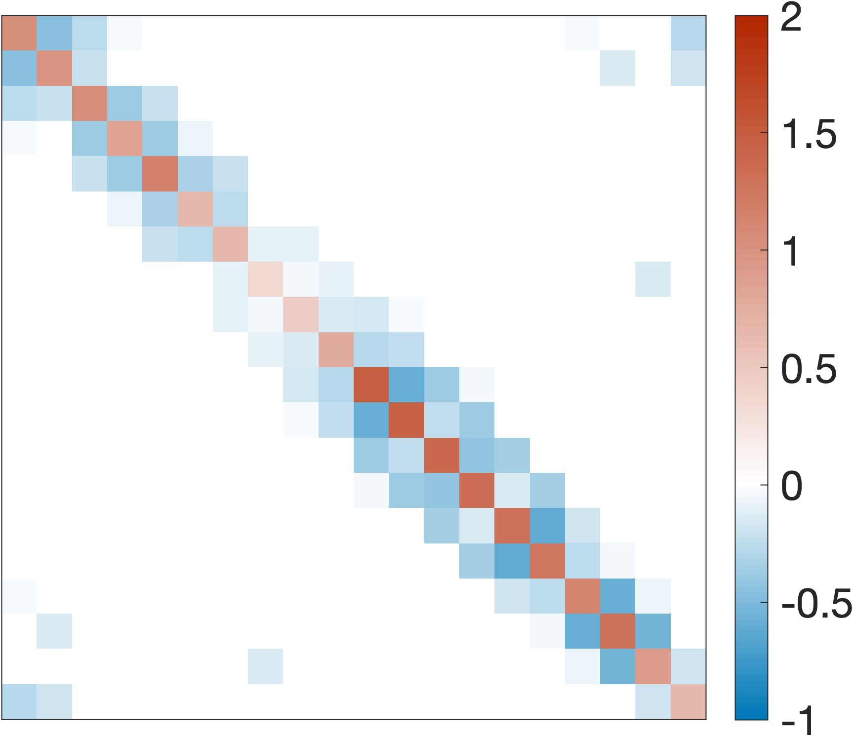
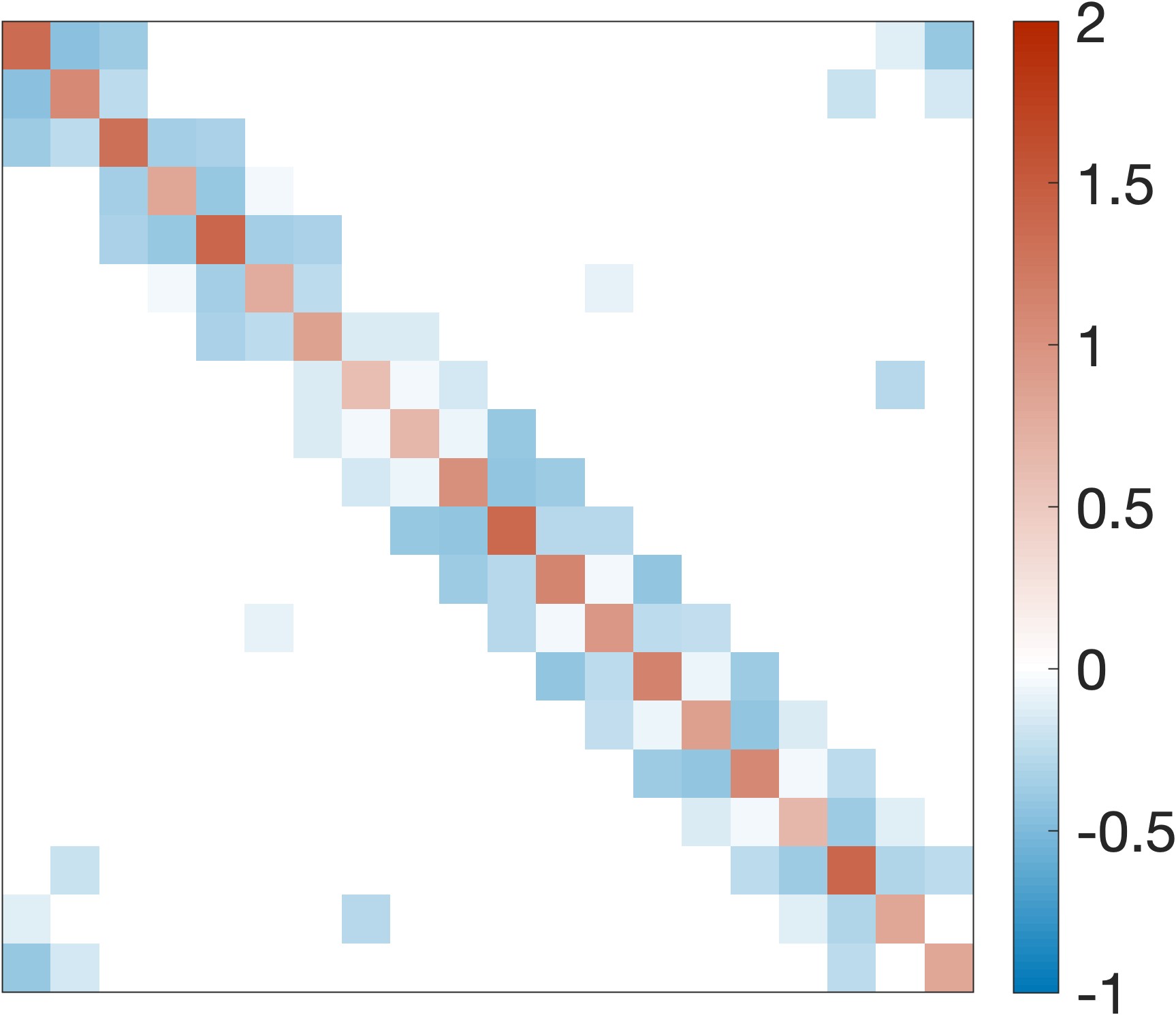
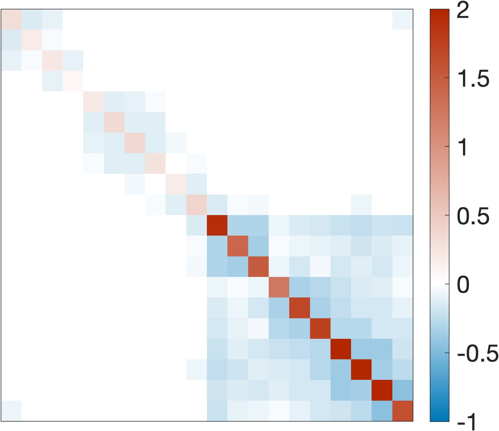
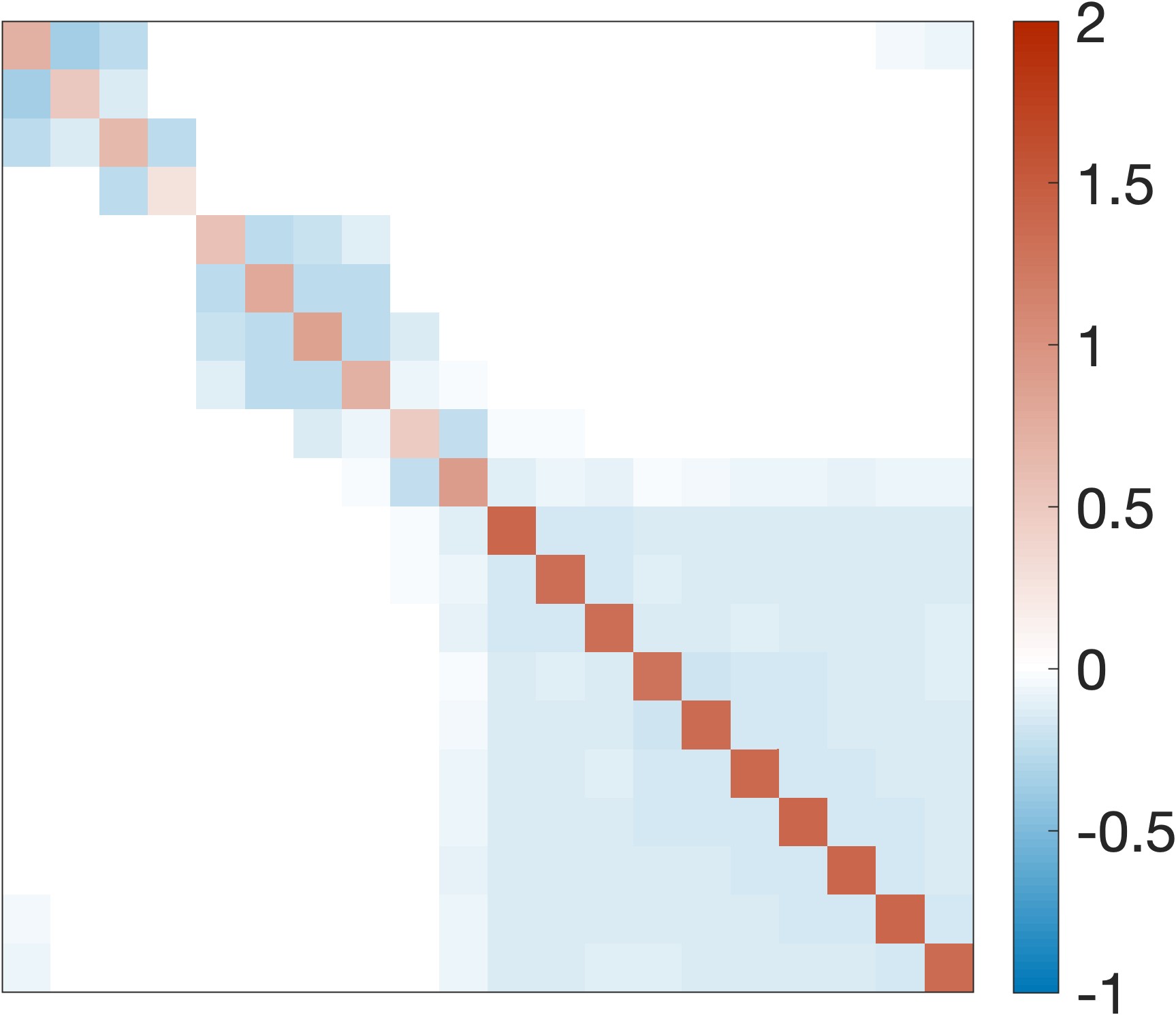
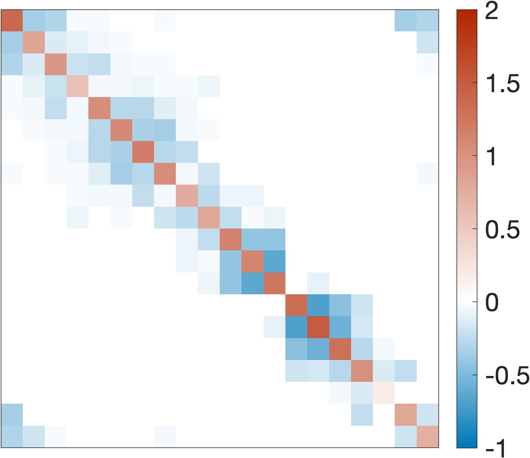
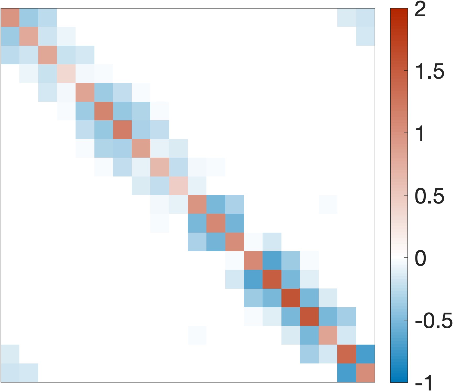
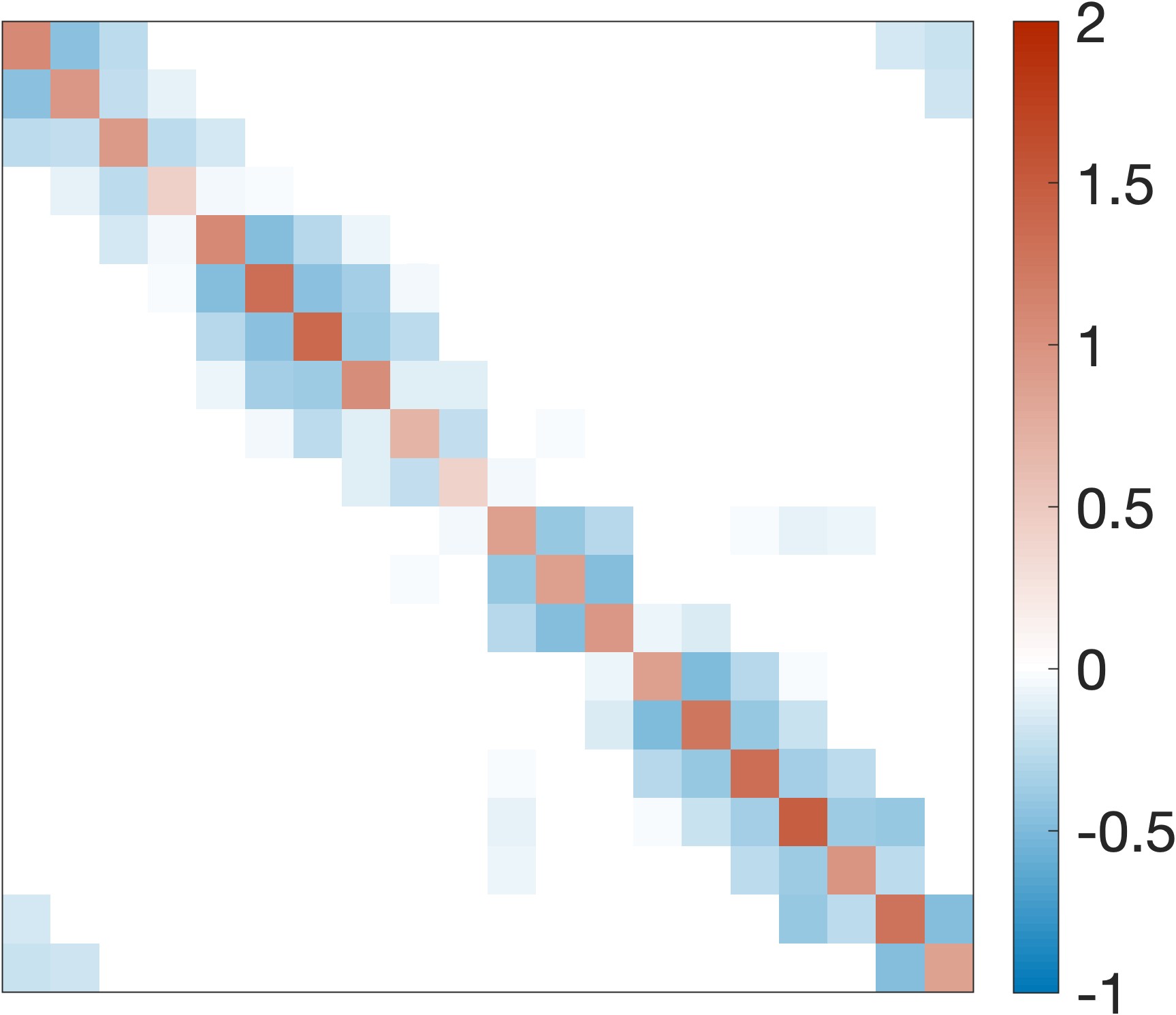
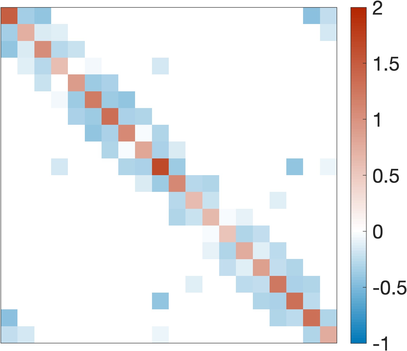
Figure 7: Graph Laplacians estimated by different methods and the ground truth Watts-Strogatz small-world graph Laplacian (K=2, p=0.1).

Appendix H Denoised Neural Signals

We visualize the average spiking activity and the averaged denoised signals for all 8 conditions in Fig. 8. The denoised signals are the exponential of learn smooth representation $Y$, which can be considered as the firing rate of neurons. Note that GLEN-TV smooth the signals both spatially and temporally.

	Average Spiking	Average Denoised Signals
$0^{\circ}$
$45^{\circ}$
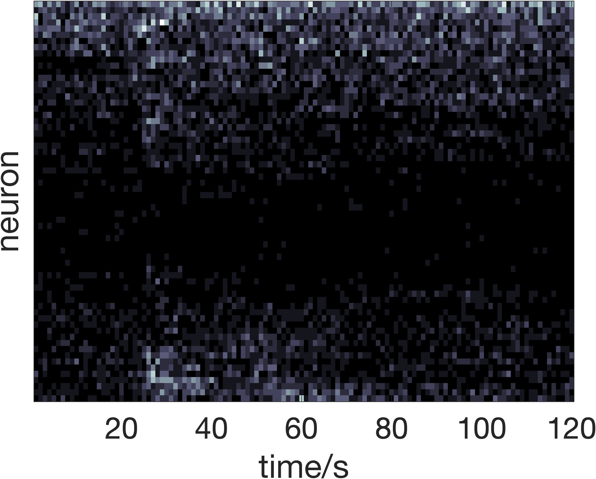
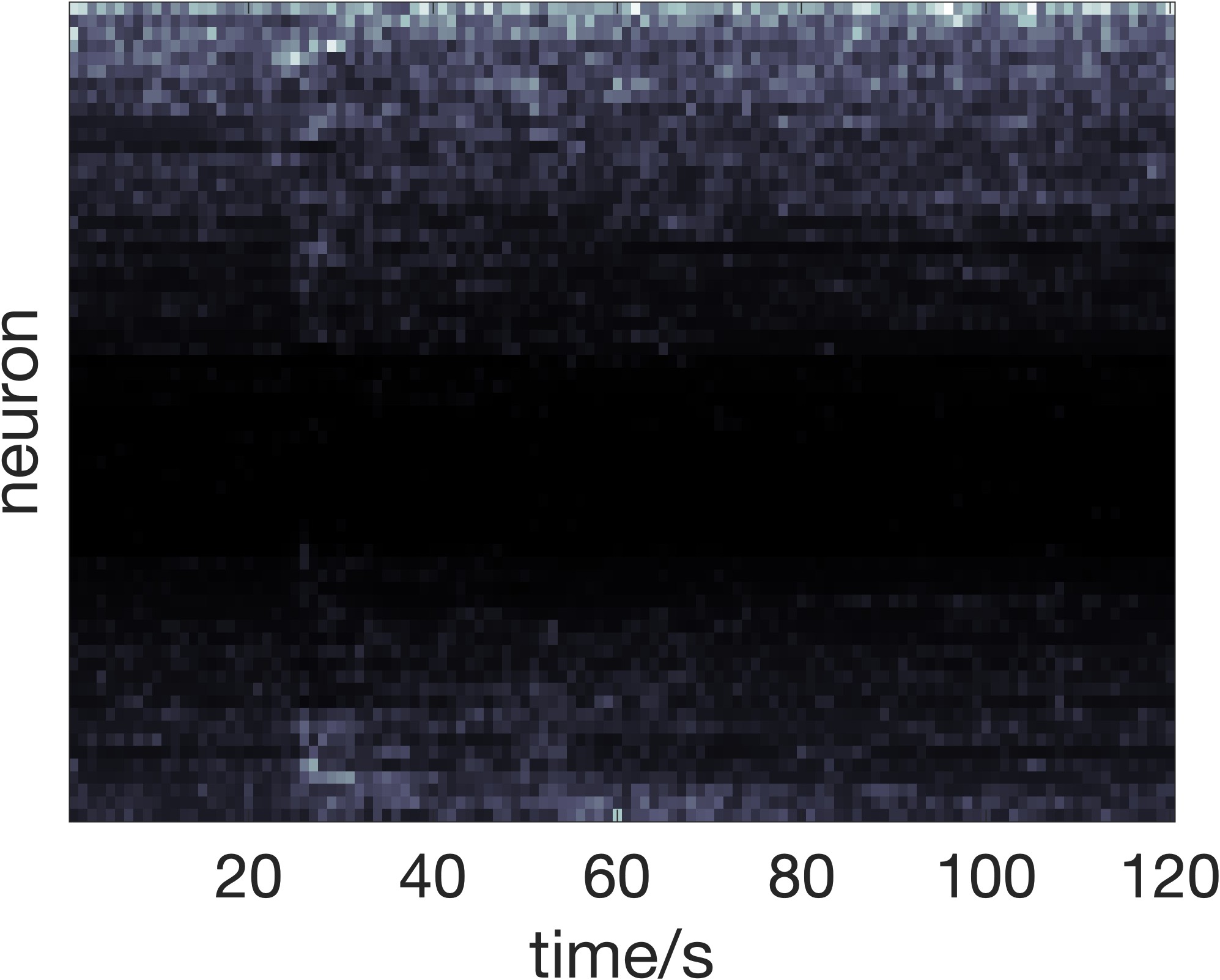
$90^{\circ}$
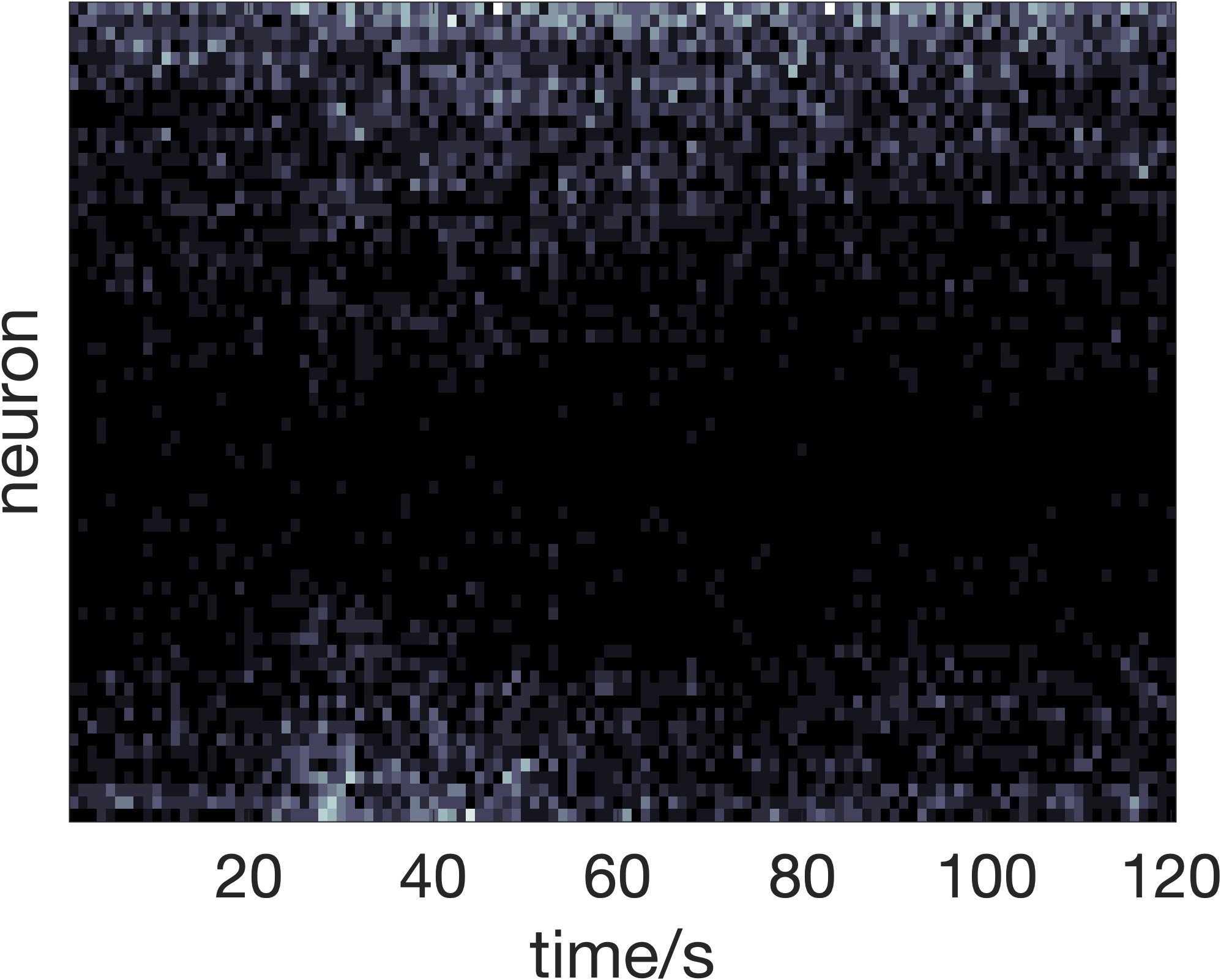
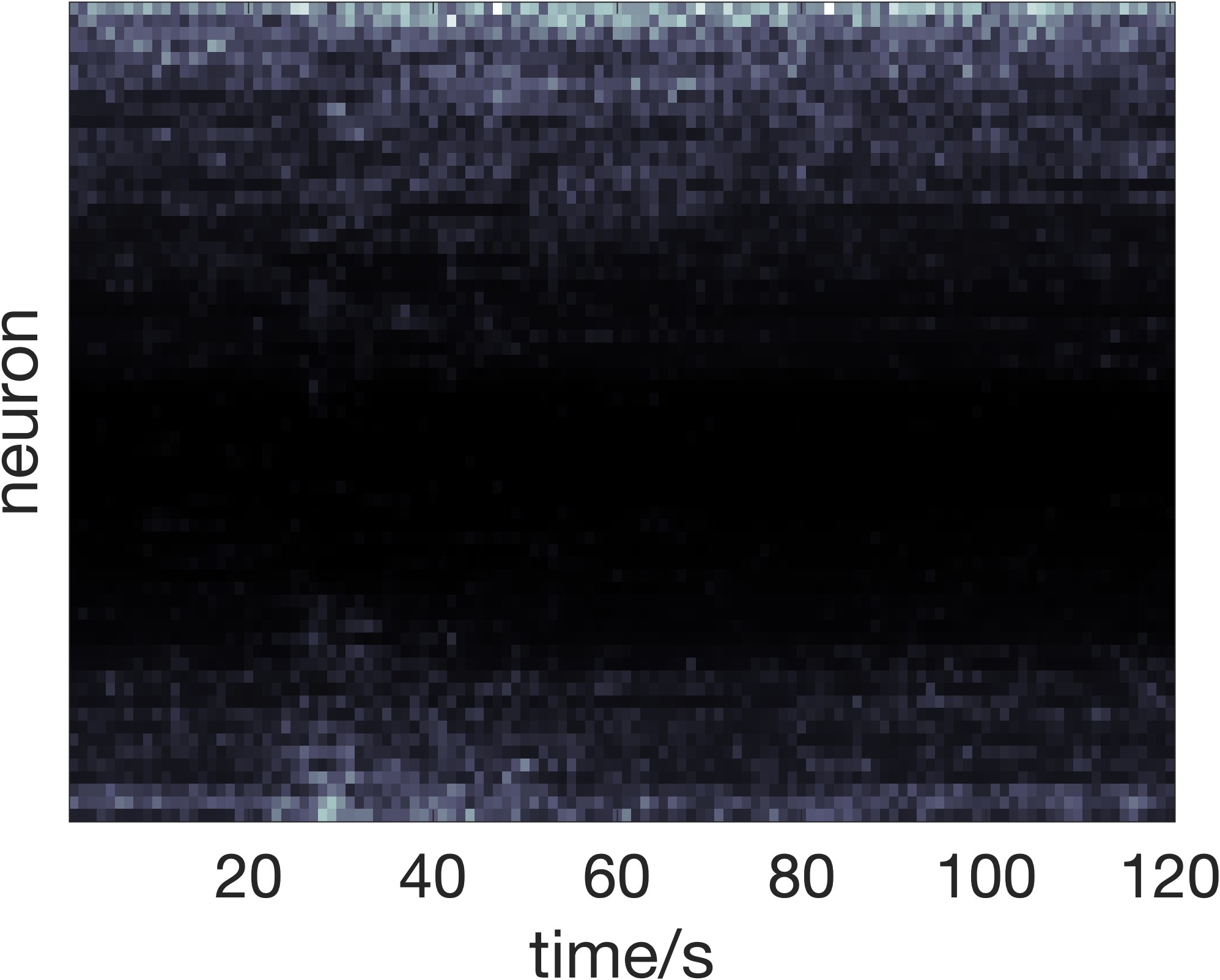
$135^{\circ}$

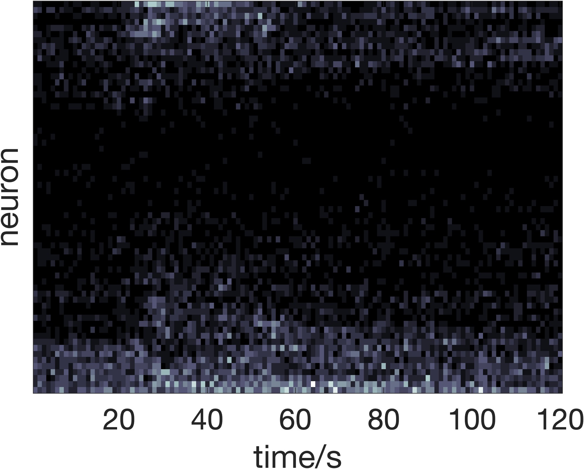
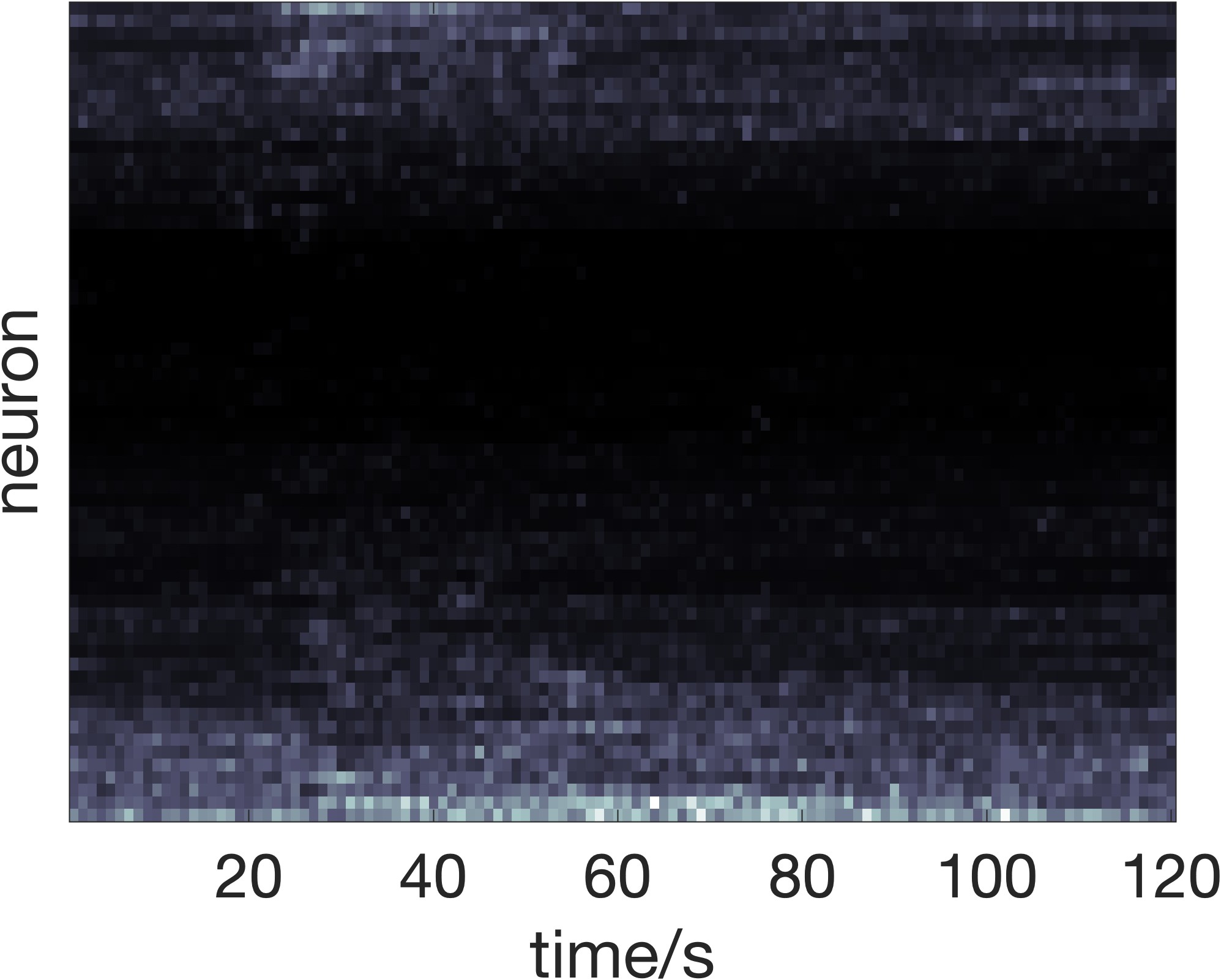
	Average Spiking	Average Denoised Signals
$180^{\circ}$
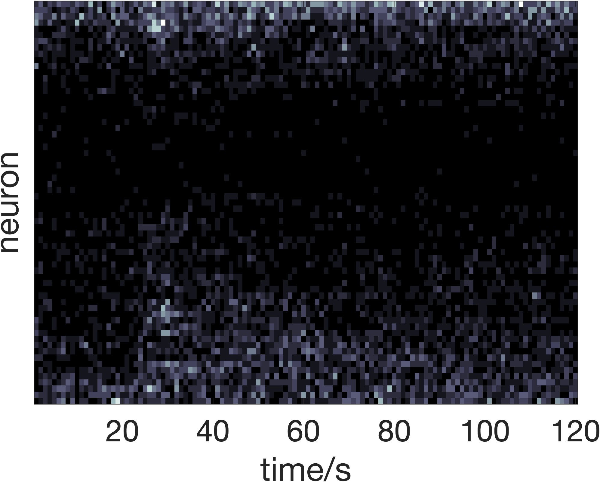
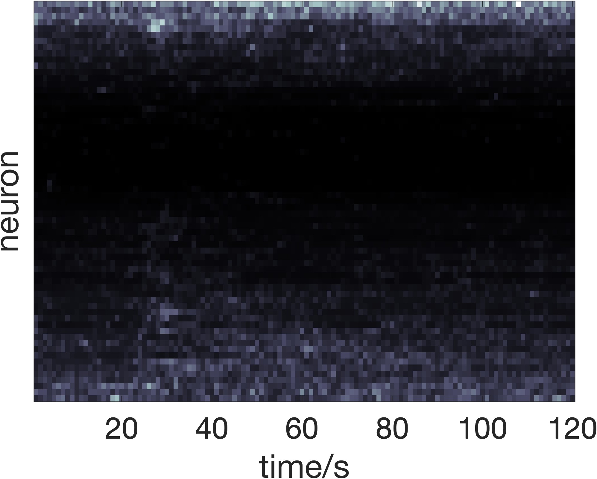
$225^{\circ}$
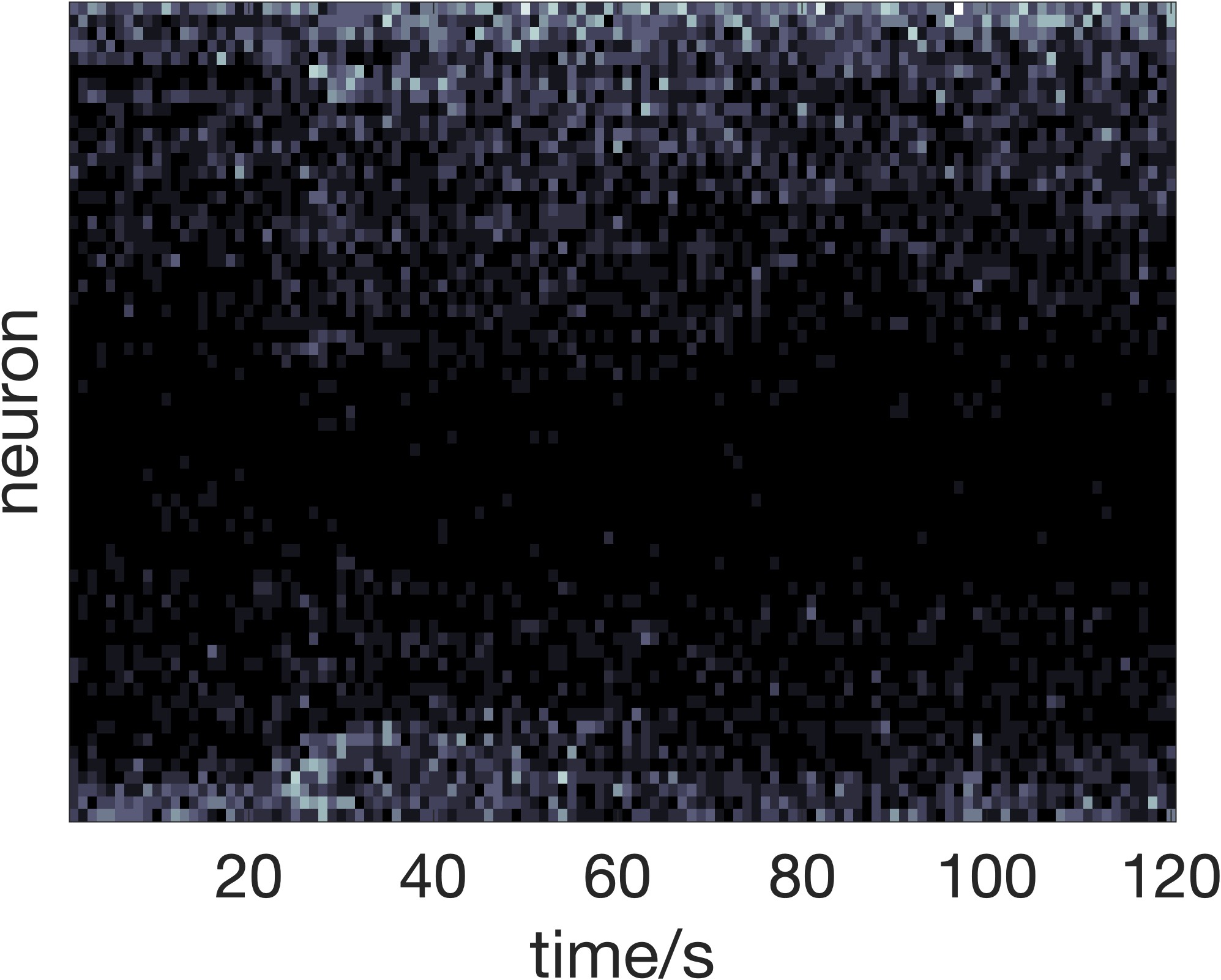
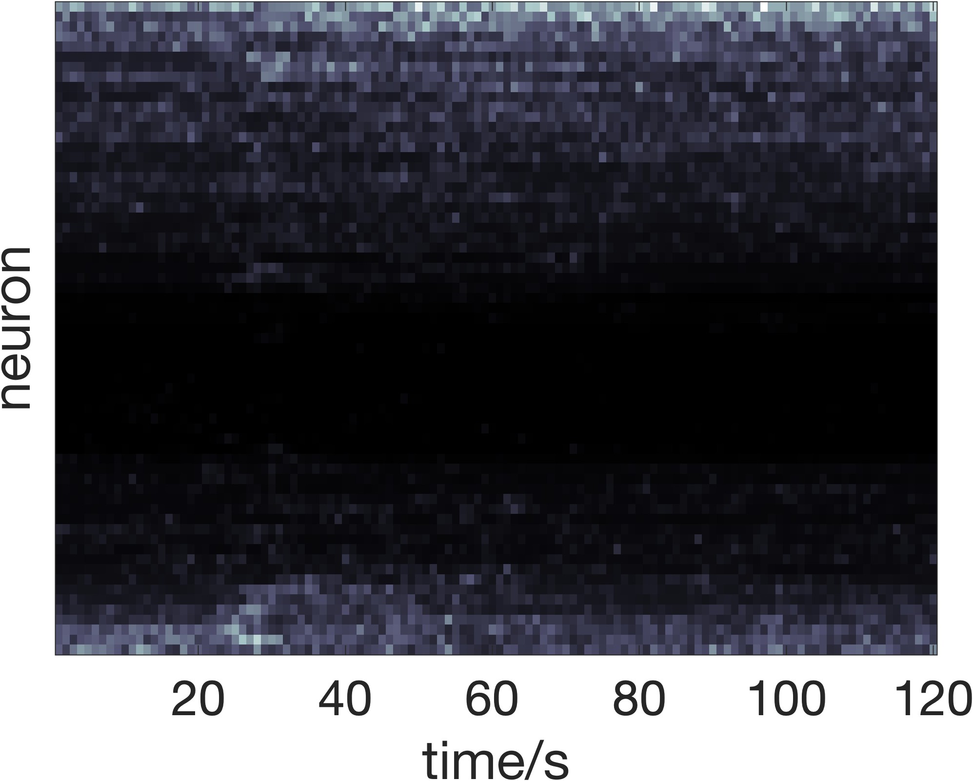
$270^{\circ}$
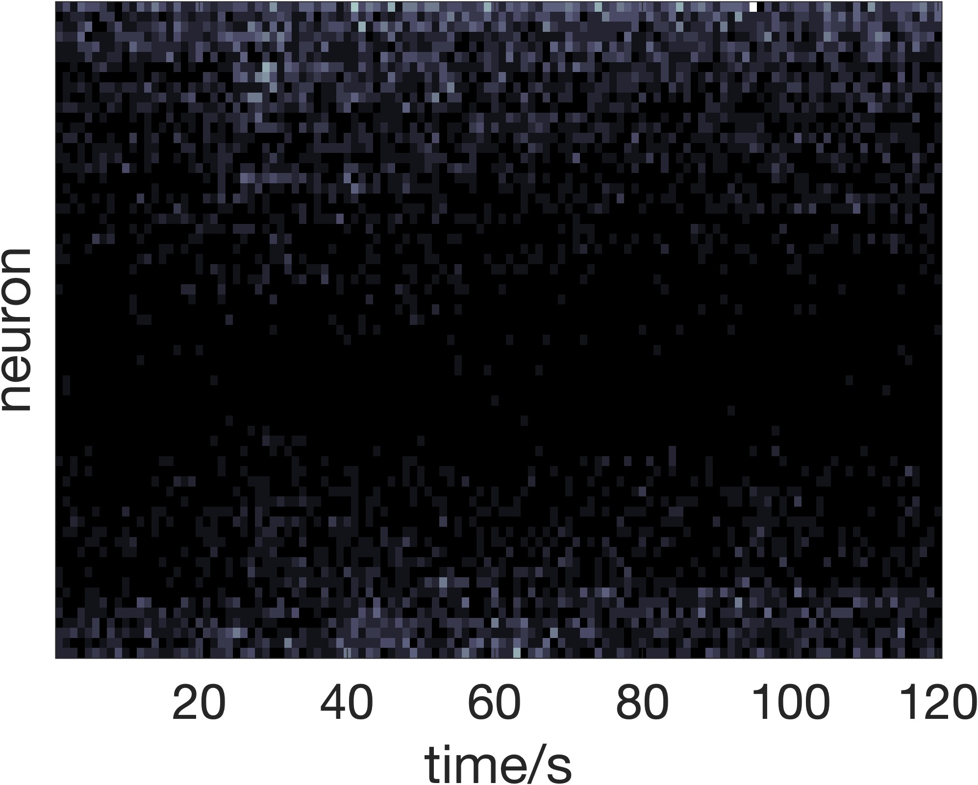
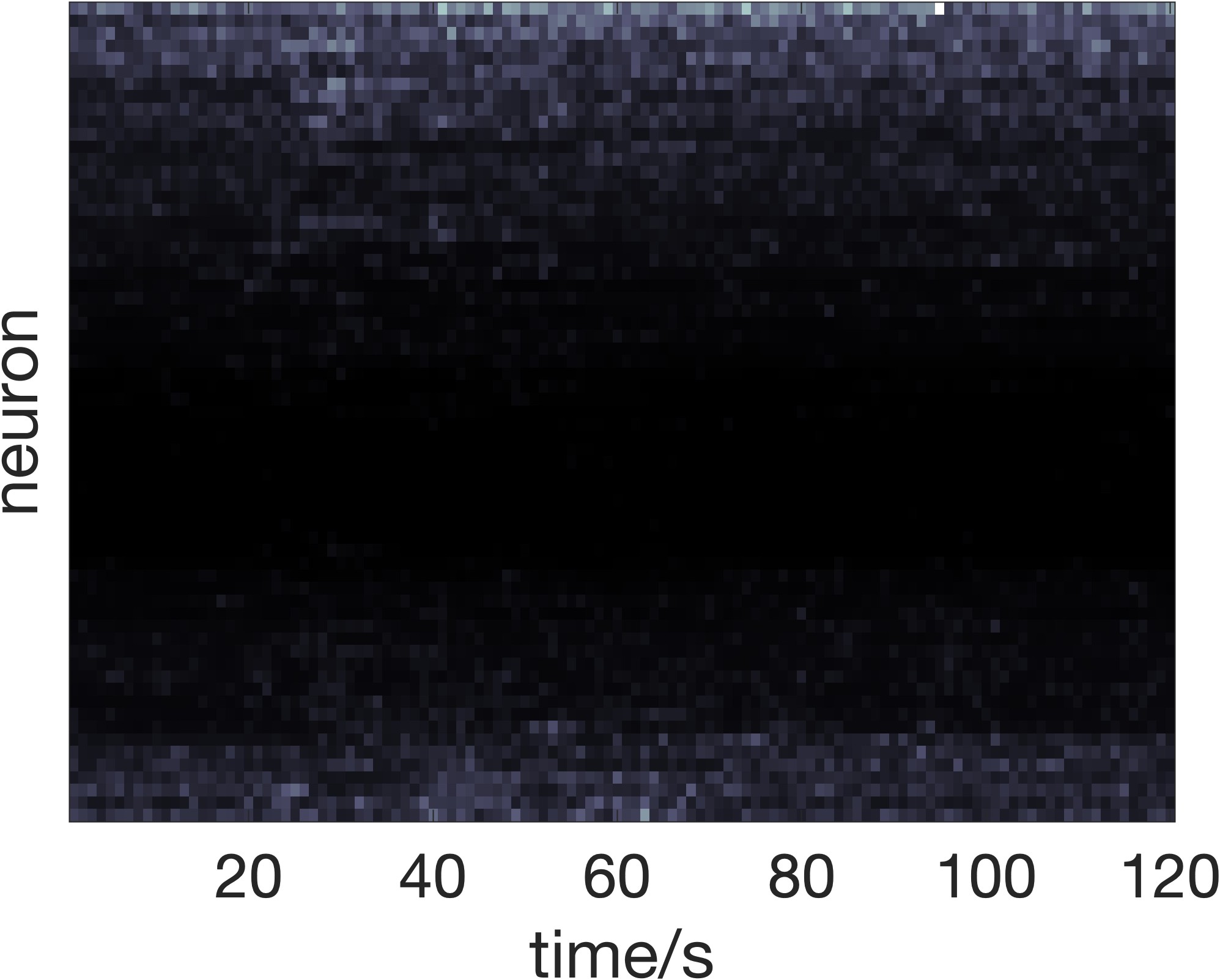
$315^{\circ}$

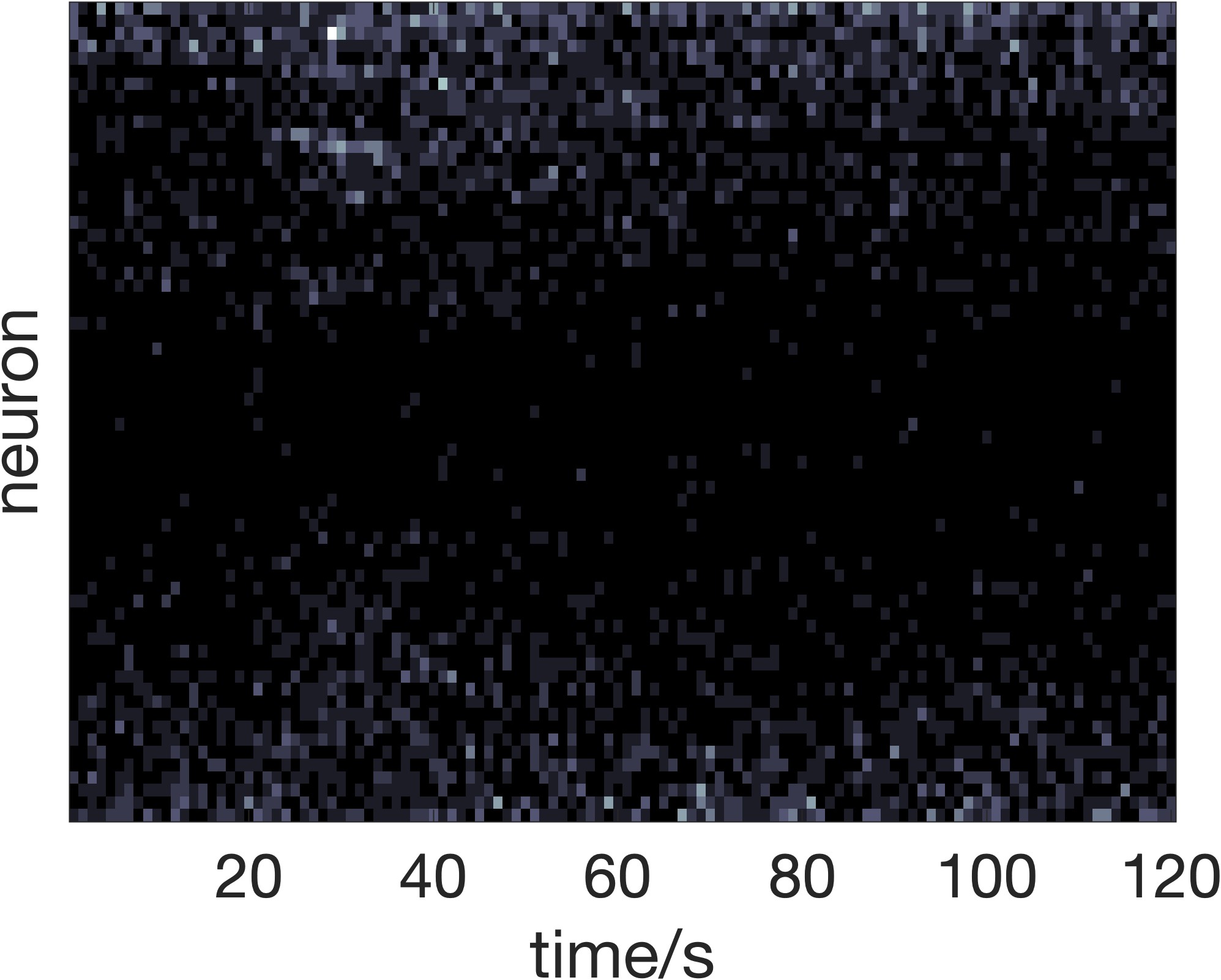
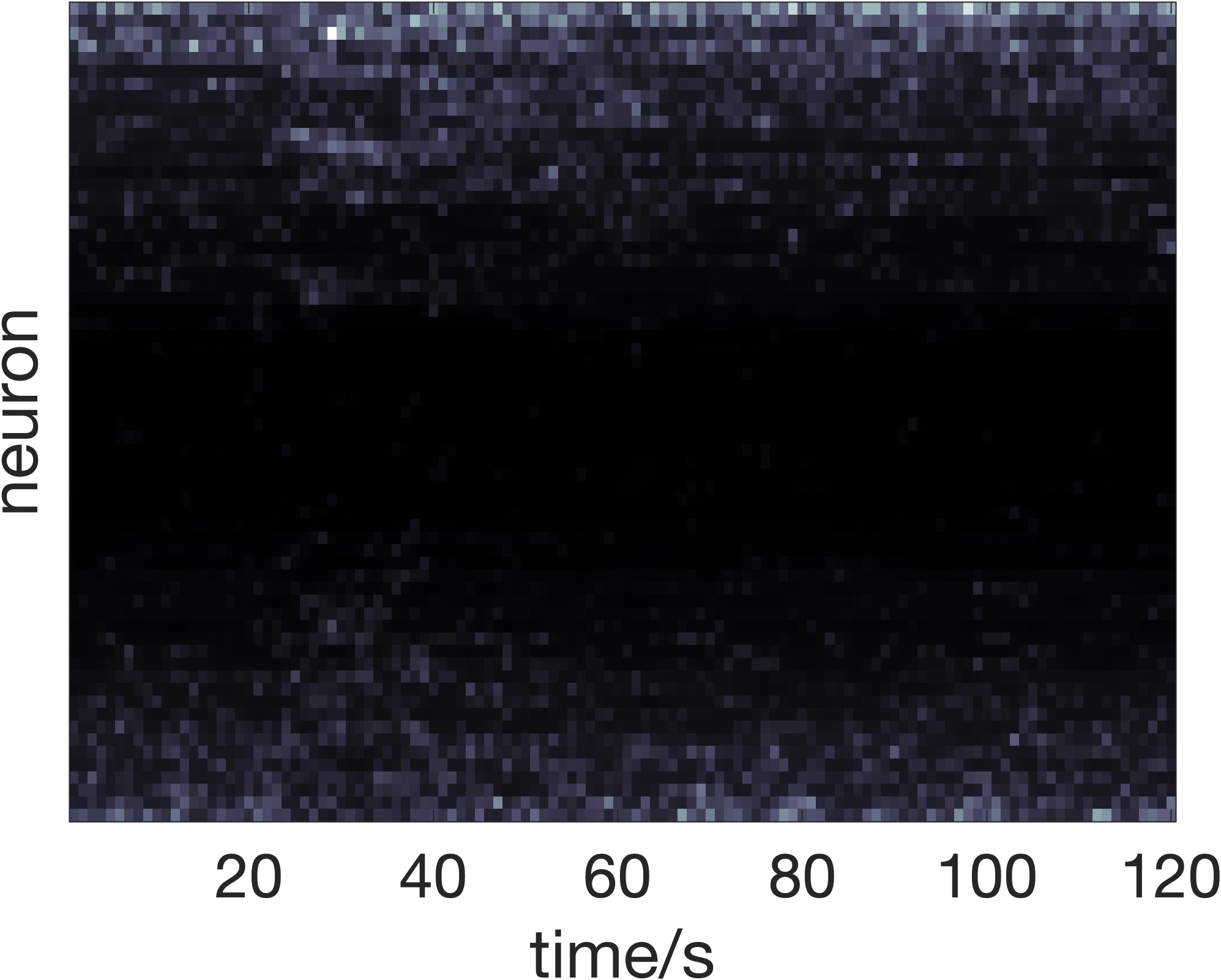
Figure 8: Average of raw neural spiking data compared against average denoised signals by GLEN-TV, for each target direction shown on the left. Brighter indicates higher firing rate.

References

- Aitchison & Ho (1989) Aitchison, J. and Ho, C. The multivariate Poisson-log normal distribution. Biometrika, 76(4):643–653, 1989.
- Aitchison & Shen (1980) Aitchison, J. and Shen, S. M. Logistic-normal distributions: Some properties and uses. Biometrika, 67(2):261–272, 1980.
- Banerjee et al. (2008) Banerjee, O., El Ghaoui, L., and d’Aspremont, A. Model selection through sparse maximum likelihood estimation for multivariate Gaussian or binary data. JMLR, 9:485–516, 2008.
- Biswas et al. (2016) Biswas, S., Mcdonald, M., Lundberg, D. S., Dangl, J. L., and Jojic, V. Learning microbial interaction networks from metagenomic count data. Journal of Computational Biology, 23(6):526–535, 2016.
- Buciulea et al. (2022) Buciulea, A., Rey, S., and Marques, A. G. Learning graphs from smooth and graph-stationary signals with hidden variables. IEEE Transactions on Signal and Information Processing over Networks, 8:273–287, 2022.
- Bullmore & Sporns (2009) Bullmore, E. and Sporns, O. Complex brain networks: graph theoretical analysis of structural and functional systems. Nature reviews neuroscience, 10(3):186–198, 2009.
- Chiquet et al. (2019) Chiquet, J., Robin, S., and Mariadassou, M. Variational inference for sparse network reconstruction from count data. In ICML, pp. 1162–1171. PMLR, 2019.
- Cipra (1987) Cipra, B. A. An introduction to the Ising model. The American Mathematical Monthly, 94(10):937–959, 1987.
- Dong et al. (2016) Dong, X., Thanou, D., Frossard, P., and Vandergheynst, P. Learning Laplacian matrix in smooth graph signal representations. IEEE Trans. Signal Process., 64(23):6160–6173, 2016.
- Dong et al. (2019) Dong, X., Thanou, D., Rabbat, M., and Frossard, P. Learning graphs from data: A signal representation perspective. IEEE Signal Process. Mag., 36(3):44–63, 2019.
- Egilmez et al. (2017) Egilmez, H. E., Pavez, E., and Ortega, A. Graph learning from data under Laplacian and structural constraints. IEEE J. Sel. Topics Signal Process., 11(6):825–841, 2017.
- Friedman et al. (2008) Friedman, J., Hastie, T., and Tibshirani, R. Sparse inverse covariance estimation with the graphical lasso. Biostatistics, 9(3):432–441, 2008.
- Grassi et al. (2017) Grassi, F., Loukas, A., Perraudin, N., and Ricaud, B. A time-vertex signal processing framework: Scalable processing and meaningful representations for time-series on graphs. IEEE Trans. Signal Process., 66(3):817–829, 2017.
- Hammond et al. (2011) Hammond, D. K., Vandergheynst, P., and Gribonval, R. Wavelets on graphs via spectral graph theory. Applied and Computational Harmonic Analysis, 30(2):129–150, 2011.
- Hu et al. (2015) Hu, C., Cheng, L., Sepulcre, J., Johnson, K. A., Fakhri, G. E., Lu, Y. M., and Li, Q. A spectral graph regression model for learning brain connectivity of Alzheimer’s disease. PloS One, 10(5):e0128136, 2015.
- Humbert et al. (2021) Humbert, P., Le Bars, B., Oudre, L., Kalogeratos, A., and Vayatis, N. Learning laplacian matrix from graph signals with sparse spectral representation. The Journal of Machine Learning Research, 22(1):8766–8812, 2021.
- Kalofolias (2016) Kalofolias, V. How to learn a graph from smooth signals. In AISTATS, pp. 920–929. PMLR, 2016.
- Kalofolias & Perraudin (2017) Kalofolias, V. and Perraudin, N. Large scale graph learning from smooth signals. arXiv preprint arXiv:1710.05654, 2017.
- Kemp & Tenenbaum (2008) Kemp, C. and Tenenbaum, J. B. The discovery of structural form. Proceedings of the National Academy of Sciences, 105(31):10687–10692, 2008.
- Kumar et al. (2020) Kumar, S., Ying, J., de Miranda Cardoso, J. V., and Palomar, D. P. A unified framework for structured graph learning via spectral constraints. JMLR, 21(22):1–60, 2020.
- Kurtz et al. (2015) Kurtz, Z. D., Müller, C. L., Miraldi, E. R., Littman, D. R., Blaser, M. J., and Bonneau, R. A. Sparse and compositionally robust inference of microbial ecological networks. PLoS Computational Biology, 11(5):e1004226, 2015.
- Lake & Tenenbaum (2010) Lake, B. and Tenenbaum, J. Discovering structure by learning sparse graphs. In Proceedings of the 32nd Annual Conference of the CSS, 2010.
- Latora & Marchiori (2002) Latora, V. and Marchiori, M. Is the boston subway a small-world network? Physica A: Statistical Mechanics and its Applications, 314(1-4):109–113, 2002.
- Liu et al. (2019) Liu, Y., Yang, L., You, K., Guo, W., and Wang, W. Graph learning based on spatiotemporal smoothness for time-varying graph signal. IEEE Access, 7:62372–62386, 2019.
- Maretic et al. (2017) Maretic, H. P., Thanou, D., and Frossard, P. Graph learning under sparsity priors. In IEEE International Conference on Acoustics, Speech and Signal Processing (ICASSP), pp. 6523–6527, 2017.
- Mateos et al. (2019) Mateos, G., Segarra, S., Marques, A. G., and Ribeiro, A. Connecting the dots: Identifying network structure via graph signal processing. IEEE Signal Process. Mag., 36(3):16–43, 2019.
- Navarro et al. (2020) Navarro, M., Wang, Y., Marques, A. G., Uhler, C., and Segarra, S. Joint inference of multiple graphs from matrix polynomials. J. Mach. Learn. Res., 23:1–35, 2020.
- Ortega et al. (2018) Ortega, A., Frossard, P., Kovačević, J., Moura, J. M., and Vandergheynst, P. Graph signal processing: Overview, challenges, and applications. Proceedings of the IEEE, 106(5):808–828, 2018.
- Park et al. (2017) Park, Y., Hallac, D., Boyd, S., and Leskovec, J. Learning the network structure of heterogeneous data via pairwise exponential Markov random fields. In AISTATS, pp. 1302–1310. PMLR, 2017.
- Pasdeloup et al. (2017) Pasdeloup, B., Gripon, V., Mercier, G., Pastor, D., and Rabbat, M. G. Characterization and inference of graph diffusion processes from observations of stationary signals. IEEE Trans. Signal Inf. Process, 4(3):481–496, 2017.
- Pei et al. (2021) Pei, F., Ye, J., Zoltowski, D., Wu, A., Chowdhury, R. H., Sohn, H., O’Doherty, J. E., Shenoy, K. V., Kaufman, M. T., Churchland, M., et al. Neural latents benchmark’21: Evaluating latent variable models of neural population activity. arXiv preprint arXiv:2109.04463, 2021.
- Perraudin et al. (2014) Perraudin, N., Paratte, J., Shuman, D., Martin, L., Kalofolias, V., Vandergheynst, P., and Hammond, D. K. Gspbox: A toolbox for signal processing on graphs. arXiv preprint arXiv:1408.5781, 2014.
- Robins et al. (2007) Robins, G., Pattison, P., Kalish, Y., and Lusher, D. An introduction to exponential random graph (p*) models for social networks. Social networks, 29(2):173–191, 2007.
- Rue & Held (2005) Rue, H. and Held, L. Gaussian Markov random fields: theory and applications. Chapman and Hall/CRC, 2005.
- Saboksayr & Mateos (2021) Saboksayr, S. S. and Mateos, G. Accelerated graph learning from smooth signals. IEEE Signal Processing Letters, 28:2192–2196, 2021.
- Sardellitti et al. (2019) Sardellitti, S., Barbarossa, S., and Di Lorenzo, P. Graph topology inference based on sparsifying transform learning. IEEE Transactions on Signal Processing, 67(7):1712–1727, 2019.
- Segarra et al. (2017) Segarra, S., Marques, A. G., Mateos, G., and Ribeiro, A. Network topology inference from spectral templates. IEEE Trans. Signal Inf. Process, 3(3):467–483, 2017.
- Sensors (2017) Sensors, B. W. S.-A. City of chicago— data portal.(nd). retrieved april 25, 2017, 2017.
- Shafipour et al. (2021) Shafipour, R., Segarra, S., Marques, A. G., and Mateos, G. Identifying the topology of undirected networks from diffused non-stationary graph signals. IEEE Open Journal of Signal Processing, 2:171–189, 2021.
- Slawski & Hein (2015) Slawski, M. and Hein, M. Estimation of positive definite M-matrices and structure learning for attractive Gaussian Markov random fields. Linear Algebra and its Applications, 473:145–179, 2015.
- Thanou et al. (2017) Thanou, D., Dong, X., Kressner, D., and Frossard, P. Learning heat diffusion graphs. IEEE Trans. Signal Inf. Process, 3(3):484–499, 2017.
- Trinajstic (2018) Trinajstic, N. Chemical graph theory. CRC press, 2018.
- Yang et al. (2012) Yang, E., Allen, G., Liu, Z., and Ravikumar, P. Graphical models via generalized linear models. Advances in neural information processing systems, 25, 2012.
- Yang et al. (2015) Yang, E., Ravikumar, P., Allen, G. I., and Liu, Z. Graphical models via univariate exponential family distributions. JMLR, 16(1):3813–3847, 2015.
- Yu et al. (2004) Yu, J., Smith, V. A., Wang, P. P., Hartemink, A. J., and Jarvis, E. D. Advances to Bayesian network inference for generating causal networks from observational biological data. Bioinformatics, 20(18):3594–3603, 2004.
- Zhang & Poole (1996) Zhang, N. L. and Poole, D. Exploiting causal independence in Bayesian network inference. JAIR, 5:301–328, 1996.