Inertial randomized Kaczmarz algorithms for solving coherent linear systems
Abstract
In this paper, by regarding the two-subspace Kaczmarz method [20] as an alternated inertial randomized Kaczmarz algorithm we present a new convergence rate estimate which is shown to be better than that in [20] under a mild condition. Furthermore, we accelerate the alternated inertial randomized Kaczmarz algorithm and introduce a multi-step inertial randomized Kaczmarz algorithm which is proved to have a faster convergence rate. Numerical experiments support the theory results and illustrate that the multi-inertial randomized Kaczmarz algorithm significantly outperform the two-subspace Kaczmarz method in solving coherent linear systems.
Keywords: System of linear equations, randomized Kaczmarz algorithm, inertial randomized Kaczmarz algorithm, inertial extrapolation, two-subspace Kaczmarz method.
1 Introduction
Let be the real vector space of -dimensional column vectors with usual inner product and norm , respectively. We consider the following system of linear equations:
| (1) |
where , and . Denote by , the row vectors of , then the linear equations in the system (1) can be expressed as , . As is known to all, associated with each equation , there is a hyperplane defined by
The orthogonal projection operator from onto the hyperplane assigns to each the unique point in closest to , denoted by (see (7) below for its closed expression).
Kaczmarz algorithm is one of the most popular methods to solve (1) (see, e.g., [15], [6, Chapter 8]), which can be expressed in terms of the operators as follows:
where . Because Kaczmarz algorithm uses only single equation at each iteration step, it is also called a row-action [5, 7] or sequential method. If the system (1) is consistent, the sequence generated by Kaczmarz algorithm converges to the solution closest to the initial value .
The convergence speed of Kaczmarz algorithm heavily depends on the ordering of the equations. In selecting the equation ordering, the important thing is to avoid particularly bad ordering, in which case the hyperplanes and are nearly parallel [13], i.e., and is highly correlated (its definition is given later). Furthermore, it is very difficult to estimate the convergence rate of Kaczmarz algorithm.
To overcome this difficulty, Strohmer and Vershynin [24] proposed the following randomized Kaczmarz algorithm.
Strohmer and Vershynin proved that Algorithm 1 converges linearly in expectation when the linear system (1) is consistent and is a full column rank matrix with . Later, Ma and Needell et al. [17] showed that whether the matrix satisfies with full column rank, or with full row rank, Algorithm 1 converges linearly in expectation to the minimum norm solution of the linear system (1). Furthermore, Gower and Richtárik [9] proved that even if the full rank assumption imposed on the matrix is removed, the convergence result of Algorithm 1 still holds. Precisely, their convergence result is as follows.
Theorem 1.1.
Highly correlated linear systems are often encountered in engineering practice, for example sampling in geophysics which is the reconstruction of a bandlimited function from nonuniformly spaced since it can be physically challenging to take uniform samples. When the sampling is expressed as a system of linear equations, the sampling points form the rows of a matrix which are close together and therefore the corresponding rows will be highly correlated.
The quantity
is generally used to measure the coherence between the rows of the matrix . The larger means the higher coherence between row vectors of . Hereafter, is called the coherence constant of , and the linear system (1) is called coherent if . It is easy to see that when is large, the convergence speed of Kaczmarz algorithm (even randomized Kaczmarz algorithm) is relatively slow, regardless of the order of equations. Therefore, it is of great significance to present accelerated versions of the randomized Kaczmarz algorithm which can effectively solve the coherent linear systems.
In [20], Needell and Ward introduced so called two-subspace Kaczmarz method based on the idea of the orthogonalization, where the matrix is standardized which means that each of its rows has unit Euclidean norm before the implementation of the method.
The convergence rate estimate was established when is a full rank standardized matrix with in [20]. In fact the full rank assumption can be removed as Theorem 1.1 and the convergence results is given as follows.
Theorem 1.2.
Assume that the linear system (1) is consistent. Let the initial guess be selected in arbitrarily. Let be the sequence generated by the two-subspace Kaczmarz method. Then
| (3) |
where and
Comparing the estimates (2) and (3), it is easy to see that the two-subspace Kaczmarz method improves the randomized Kaczmarz algorithm if any rows of are highly correlated.
The inertial extrapolation firstly introduced by Polyak [22] has been widely used to accelerate the convergence speed of iterative algorithms (see, e.g., [8] and [11]) since the cost of each iteration stays basically unchanged. To introduce the inertial extrapolation, we start by introducing the term “basic algorithm”. Consider the algorithmic operator working iteratively by
| (4) |
which is denoted as the basic algorithm. The inertial version of the basic algorithm (4) is defined as follows:
| (5) |
where is referred to as the inertial term and as the inertial parameter. The main feature of inertial type methods is that the next iterate is defined by making use of the previous two iterates. The inertial parameter sequence is key to inertial type algorithms and a careful choice is known to accelerate the convergence rate of the objective function from to or for a large class of first-order algorithms of the convex optimization (see [1, 4, 21] for details). Since its inception, inertial type method has received a great deal of attention of many authors, who improved it in various ways. Mu and Peng [18] firstly introduced alternated inertial methods applying inertia every other iteration, which was extended to solve the composite convex optimization problem [14] and variational inequalities [23]. Recently multi-step inertial methods [16] were proposed based on the idea of using previous more than two iterates to accelerate the convergence rate.
The purpose of this paper is three folds. Firstly, we give a new convergence rate estimate of the two-subspace Kaczmarz method by rewriting it as an alternated inertial randomized Kaczmarz algorithm and show that it is better than that in [20] under a mild condition. Secondly, we introduce a multi-step inertial randomized Kaczmarz algorithm by combining the inertial extrapolation and the randomized Kaczmarz algorithm and its convergence rate is proved to be faster than the two-subspace Kaczmarz method. Finally, numerical experiments support the theory results and illustrate that the proposed algorithm outperform the two-subspace Kaczmarz method in solving coherent linear systems.
The paper is structured as follows. In the next section, we introduce some fundamental concepts and tools, which are needed in the subsequent sections. In Section 3, we rewrite the two-subspace Kaczmarz method as the alternated inertial randomized Kaczmarz algorithm and present a new convergence rate. In Section 4, we propose the multi-step inertial randomized Kaczmarz algorithm as a further extension of the alternated inertial randomized Kaczmarz algorithm. Numerical experiments are presented in Section 5 to show the efficiency and advantage of our proposed algorithm.
2 Preliminaries
In this section, some fundamental tools are listed that will be used in the convergence analysis of the proposed methods.
We will use the following notations:
-
and denote two index sets, respectively.
-
denotes the minimum nonzero eigenvalue of .
-
denotes the Frobenius norm of .
-
and denote two constants, respectively.
-
denotes the minimum norm solution of the problem (1).
-
and denote the full expectation and the conditional expectation of a random variable, respectively.
For a given nonempty closed convex subset of , the projection operator onto is the mapping from to that assigns to each the unique point in , denoted , closest to that is,
A subset of is called a hyperplane if is of the form
| (6) |
where is a fixed nonzero vector in and is a number in . Obviously, a hyperplane is closed and convex, and we have the following closed-form formula for projections onto a hyperplane (see [3, Chapter 25] or [12]).
Lemma 2.1.
Let be a hyperplane of the form (6). Then, for any , we have
| (7) |
In what follows, we denote by the projection operator onto
The following property is a well-known characterization of projections.
Lemma 2.2.
([10, Section 3]) Let be a closed convex subset of Given and . Then if and only if
| (8) |
Moreover, if is a hyperplane, then if and only if
| (9) |
Lemma 2.3.
Throughout the rest of this paper, all discussions are based on the following two basic assumptions:
-
(H1)
The system of linear equations (1) is consistent, that is, its solution set, denoted by , is nonempty.
- (H2)
3 Alternated inertial randomized Kaczmarz algorithm
In this section, we will give a better convergence rate estimate of the two-subspace Kaczmarz method than (3) by regarding it as an alternated inertial randomized Kaczmarz algorithm.
To this end, we first introduce an alternated inertial randomized Kaczmarz algorithm as follows.
| (11) |
| (12) |
| (13) |
Remark 3.1.
We give three important characteristics of Algorithm 3.
(i) given by (12) is well-defined for all . Indeed, since can be guaranteed by Algorithm 3, it is easy to see that under the assumption (H2).
(ii) Algorithm 3 is essentially an alternated inertial algorithm. In fact, from (11) and (7), we get
| (14) |
Obviously, in the case where , we have
| (15) |
where
| (16) |
Consequently, (13) can be rewritten as the form
| (17) |
The formula (17) means that there is an inertial extrapolation in . Since there is no inertial extrapolation in , Algorithm 3 is an alternated inertial algorithm.
(iii) When is standardized, it is easy to verify that Algorithm 3 equals to the two-subspace Kaczmarz method. The reason that we prefer the form of Algorithm 3 instead of the two-subspace Kaczmarz method in this section is that the former is convenient for us to make full use of the properties of the projection operator to analyze the convergence rate more precisely, which can be seen from Lemma 3.1 and its proof below.
We now give the following fundamental result, which is crucial to estimate the convergence rate of Algorithm 3.
Lemma 3.1.
Let be the sequence generated by Algorithm 3. Then for any and , the following statements hold:
-
(i)
-
(ii)
;
-
(iii)
;
-
(iv)
The inertial parameter sequence in (12) is optimal in the sense that makes obtain its minimum value;
-
(v)
-
(vi)
Proof.
| (18) | ||||
(ii) From (14), we have
(iii) Noting , this conclusion is a direct consequence of (14).
(iv) Obviously, in order to make Algorithm 3 obtain the optimal convergence rate, for the current , should be chosen such that reaches its minimum value. To show that the inertial parameter sequence in (12) is optimal, it suffices to verify that
holds for all .
Similar to the derivation of (18), we get
Using (iii), one has
On the other hand,
Combining above three equalities, we have
| (19) | ||||
Set
| (20) | ||||
For the current iterate , noting that
is a constant, it is easy to see from (19) and (20) that, reaching its minimum value is equivalent to the function reaching its minimum value. Note that is a quadratic function of , therefore, minimizing yields that the th optimal inertial parameter is given by (12).
(v) The conclusion can be obtained directly by setting in (19).
Remark 3.2.
(i) Lemma 3.1 (iv) provides a reference for us to find , whose idea is just the selection strategy of inertial parameters in some inertial type algorithms.
(ii) The accelerating convergence effect of Algorithm 3 can be clearly shown by (v) and (vi) of Lemma 3.1. In fact, the iterative sequence generated by Algorithm 1 only holds
and
While, due to the inertia extrapolation, the iterative sequence generated by Algorithm 3 has smaller and bigger . Indeed, from (v) and (vi) of Lemma 3.1, we get
and
Obviously, the larger , the better the acceleration effect of Algorithm 3.
Finally we analyze the convergence rate of Algorithm 3, i.e, the two-subspace Kaczmarz method as follows.
Theorem 3.1.
Choose arbitrarily and let be a sequence generated by Algorithm 3. Then converges linearly in expectation to the minimum norm solution . Precisely, for all , there holds the convergence rate estimate:
| (22) |
Proof.
Without losing generality, we assume that the system of equations (1) has been standardized, that is, holds for each . In this case, it is very easy to see that , , and hold. Consequently, Step 1 of Algorithm 3 is to select uniformly at random, i.e., with probability .
Note that holds for all , we have from (i) and (v) of Lemma 3.1 that
| (23) |
and
| (24) |
hold for all , respectively. By (24) and the definition of conditional expectation, we have
Although Algorithm 3 is equivalent to the two-subspace Kaczmarz method when is standardized, the proof of Theorem 3.1 is completely different from that of Theorem 1.2, and the former is simpler. Furthermore, the convergence rate estimate (22) and (3) are different and obviously, (22) is better than (3) in at least two aspects:
- (i)
- (ii)
Further, we can prove that (22) is better than (3) under a mild condition.
Proof.
For convenience, we assume that the system of equations (1) has been standardized, i.e., for all . Also, and are simply expressed as and , respectively. Hence (22) and (3) become
| (31) |
and
| (32) |
respectively. Note that
to prove the desired conclusion, from (31) and (32), we need to show that
| (33) |
holds for all Since and , to show (33), it suffices to verify
that is,
| (34) |
Define a real function:
| (35) |
It is easy to verify that obtains its minimum value at and this implies that proving (34) is equivalent to proving . To prove , from (35), it suffices to verify that
| (36) |
holds. Indeed, it is very easy to verify that (36) is equivalent to the condition This completes the proof. ∎
Remark 3.3.
A great deal of matrices satisfy the condition , for example, the row full rank matrix, and column full rank matrix with .
4 Multi-step inertial randomized Kaczmarz algorithm
The alternated inertial randomized Kaczmarz algorithm is computationally efficient and simple to implement, but this method still could be accelerated. In this section, we accelerate the alternated inertial randomized Kaczmarz algorithm based on the idea in multi-step inertial algorithms and thus name it as the multi-step inertial randomized Kaczmarz algorithm.
| (37) |
| (38) |
| (39) |
| (40) |
Remark 4.1.
There are two illustrations to Algorithm 4.
(i) Algorithm 4 is essentially a multi-step inertial algorithm. For each , noting , we get
| (41) |
It is easy to see from (39) and (41) that, in the case , (39) can be rewritten as the form:
| (42) |
where
| (43) |
Consequently, (40) is of the form:
| (44) |
It is easy to see from (42) and (44) that constructing involves , hence Algorithm 4 is a multi-step inertial algorithm (see, e.g. [8]).
Lemma 4.1.
The inertial parameter sequence in (38) is optimal in the sense that, for each , makes obtain its minimum value for arbitrary .
Proof.
Lemma 4.2.
Let be the sequence generated by Algorithm 4. Then for any and , the following statements hold:
-
(i)
(51) -
(ii)
(52)
Proof.
Theorem 4.1.
Choose arbitrarily and let be a sequence generated by Algorithm 4. Then converges linearly in expectation to the minimum norm solution . Precisely, for all , there holds the following statement:
| (54) |
Proof.
| (55) | ||||
For any , from (51), we have
| (56) |
From Step 1 of Algorithm 4 and (56), we get
| (57) | ||||
On the other hand, from (47), it yields . This together with Lemma 2.3 leads to
| (58) | ||||
Combining (57) and (58), it yields
| (59) |
Hence, taking the full expectation at both sides of (60), we obtain
| (60) |
Using mathematical induction, (54) follows from (55) and (60). ∎
Remark 4.2.
5 Numerical Results
In this section, we perform several experiments to compare the convergence speed of the multi-step inertial randomized Kaczmarz algorithm (denoted as MIRK) with that of the two-subspace Kaczmarz method (denoted as TSK).
We use “IT” and “CPU” to represent the arithmetical averages of the required numbers of iteration steps required and the elapsed CPU times taken to run the algorithms 50 times, respectively. The speed-up of MIRK against TSK is defined by
To test methods, we construct various types of matrices and set the entries of to be independent identically distributed uniform random variables on some interval . Changing the value of will appropriately change the coherence of .
In the implementation of the methods, we use the function to randomly generate a solution vector , and take the right-hand side as . This ensures that the randomly generated matrices constitute a solvable system of equations . For each matrix construction, two algorithms are run with the initial vector and the same fixed matrix, and terminated once the relative solution error, defined by
at the current , satisfies . In addition, all experiments are carried out using MATLAB (version R2018a) on a personal computer with 2.30 GHz central processing unit (Intel(R) Core(TM) i5-6300HQ CPU), 12.00GB memory, and Windows operating system (Windows 10).
| 0.9 | 0.5 | 0.1 | -0.4 | ||
| TSK | CPU | 3.5000 | 3.3125 | 3.1719 | 2.2188 |
| IT | |||||
| MIRK | CPU | 2.4844 | 2.4688 | 2.4063 | 2.2031 |
| IT | |||||
| speed-up | 1.4088 | 1.3417 | 1.3182 | 1.0071 | |
| 0.9 | 0.5 | 0.1 | -0.2 | ||
| TSK | CPU | 3.4531 | 3.3594 | 2.9375 | 2.7031 |
| IT | |||||
| MIRK | CPU | 2.7969 | 2.7344 | 2.6563 | 2.6250 |
| IT | |||||
| speed-up | 1.2346 | 1.2286 | 1.1059 | 1.0298 | |
(a)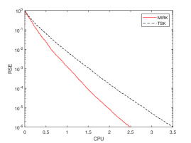 (b)
(b)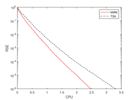 (c)
(c)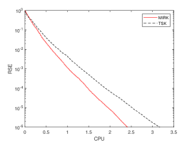 (b)
(b)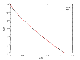
(a)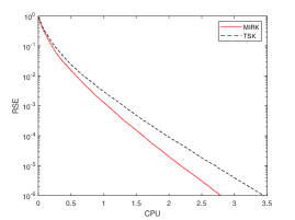 (b)
(b)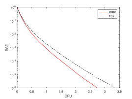 (c)
(c)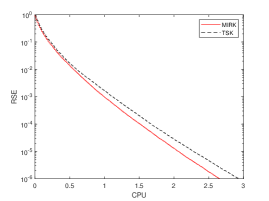 (b)
(b)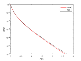
(a)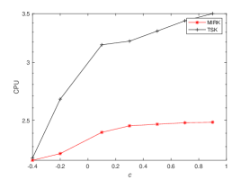 (b)
(b)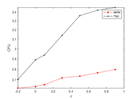
(a) (b)
(b)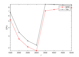
We firstly take the matrix sizes as and , and change the values of . The numbers of iteration steps and the computing times for both MIRK and TSK methods are reported in Tables 1-2, from which we see that the MIRK algorithm always outperforms the TSK method for big in terms of CPU time, whether is fat or thin. According to the data, the speed-up becomes larger as goes close to 1. When the matrix is fat, the maximum speed-up can be 1.4088. When the matrix is thin, the maximum speed-up can be 1.2346. The data in Tables 1-2 is displayed directly in Figures 1-2 which depict the curves of the relative solution error versus CPU time for the different rows and columns of matrix and different values of . It can be concluded from the figures that when , the two methods have the largest difference in the decay of the relative solution error and the MIRK algorithm is obviously better than the TSK method. The improvement effect of the MIRK algorithm over the TSK method is weakened when successively decreases or even takes a negative value. It is observed that the drop curves almost coincide in Figure 1(d) () and Figure 2(d) (), which means that the improvement effect disappears. These can also be seen in Figure 3, which illustrats that the bigger is, the more obvious improvement effect of the MIRK algorithm over the TSK method.
| 2000 | 3000 | 4000 | 5000 | ||
| TSK | CPU | 4.2719 | 3.4356 | 8.9900 | 10.5266 |
| IT | |||||
| MIRK | CPU | 3.0731 | 2.5031 | 6.7650 | 7.8109 |
| IT | |||||
| speed-up | 1.3901 | 1.3725 | 1.3289 | 1.3477 | |
| 2000 | 3000 | 4000 | 5000 | ||
| TSK | CPU | 3.3872 | 2.1891 | 8.8016 | 8.6222 |
| IT | |||||
| MIRK | CPU | 2.7056 | 1.8053 | 7.4206 | 7.8966 |
| IT | |||||
| speed-up | 1.2519 | 1.2126 | 1.1861 | 1.0919 | |
(a)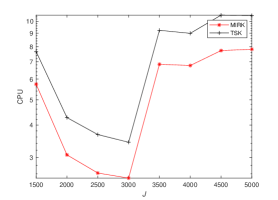 (b)
(b)
We also fix and observe the performance of two algorithms for different row and and column of . We set and change the values of in Table 3, which shows that in the fat case the speed-up can attain at most 1.3901 and least 1.3289. We fix and change the values of in Table 4 which illustrates that in thin case, the speed-up can be at most 1.2519 and at least 1.0919. It is concluded that the improvement effect is better for the fat case and decreases as becomes fatter or thinner. The above observations are visually plotted in Figure 4 which shows that the curves of the CPU time versus or of the MIRK algorithm are always lower than those of the TSK method no matter what the size of the matrix is.
6 Some concluding remarks
In this paper, we firstly give a new convergence rate of the two-subsapce Kaczmarz method by regarding it as an alternated inertial randomized Kaczmarz algorithm. Secondly, we provide a multi-step inertial randomized Kaczmarz algorithm which accelerates the alternated inertial randomized Kaczmarz algorithm. The preliminary numerical examples are presented to support the theory results.
References
- [1] Attouch, H., Peypouquet, J., The rate of convergence of Nesterov’s acclerated forward-backward method is actually faster than , SIAM J. Optim. 26(3), (2016), 1824–1834.
- [2] Bai, Z.Z., Wu, W.T., On greedy randomized Kaczmarz method for solving large sparse linear systems, SIAM J. Sci. Comput., 40, (2018), A592-A606.
- [3] Bauschke, H.H., Combettes, P.L., Convex analysis and monotone operator theory in Hilbert spaces. Springer 2010.
- [4] Beck, A., Teboulle, M., A fast iterative shrinkage-thresholding algorithm for linear inverse problems, SIAM J. Imaging Sci. 2(1)(2009), 183–202.
- [5] Browne, J., DePierro, A., A row-action alternative to the EM algorithm for maximizing likelihoods in emission tomography, IEEE Trans. Med. Imag. 15, (1996), 687–699.
- [6] Byrne, C.L., Iterative Optimization in Inverse Problems. CRC Press, Boca Raton (2014).
- [7] Censor, Y., Row-action methods for huge and sparse systems and their applications. SIAM Review. 23, (1981), 444–464.
- [8] Dong, Q.L., Huang, J., Li, X.H., Cho, Y.J., Rassias, Th.M., MiKM: Multi-step inertial Krasnosel’skiǐ–Mann algorithm and its applications, J. Global Optim. 73(4), (2019), 801–824.
- [9] Gower, R. M., Richtárik, P., Stochastic dual ascent for solving linear systems, arXiv: 1512.06890(2015), 28pages.
- [10] Goebel, K., Reich, S., Uniform convexity, hyperbolic geometry and non-expansive mappings. M. Dekker (1984).
- [11] Goldstein, T., O’Donoghue, B., Setzer, S., Baraniuk, R., Fast alternating direction optimization methods, SIAM J. Imaging Sc., 7(3), (2014), 1588–1623.
- [12] He, S.N., Yang, C.P., Duan, P.C., Realization of the hybrid method for Mann iterations. Applied Mathematics and Computation. 217, (2010), 4239–4247.
- [13] Herman, G.T., Meyer, L., Algebraic reconstruction technique can be made computationlly efficient, IEEE T. Med. Imaging, 12, (1993), 600–609.
- [14] Iutzeler, F., Malick, J., On the proximal gradient algorithm with alternated inertia, J. Optimiz. Theory App. 176, (2018), 688–710.
- [15] Kaczmarz, S., Angenäherte Auflösung von Systemen linearer Gleichungen, Bull. Int. Acad. Polon. Sci. Lett. A, 35, (1937), 355–357.
- [16] Liang, J.W., Convergence Rates of First–Order Operator Splitting Methods. Optimization and Control [math.OC]. Normandie Université; GREYC CNRS UMR 6072, 2016. English.
- [17] Ma, A., Needell, D., Ramdas, A., Convergence properties of the randomized extended Gauss-Seidel and Kaczmarz methods, SIAM J. Matrix Anal. Appl., 36, (2015), 1590–1604.
- [18] Mu, Z., Peng, Y., A note on the inertial proximal point method, Stat. Optim. Inf. Comput. 3, (2015), 241–248.
- [19] Needell, D., Tropp, J.A., Paved with good intentions: analysis of a randomized block Kaczmarz method, Linear Algebra Appl. 441, (2014), 199–221.
- [20] Needell, D., Ward, R., Two-subspace projection method for coherent overdetermined systems, J. Fourier Anal. Appl., 19, (2013), 256–269.
- [21] Nesterov, Y.E., A method for solving the convex programming problem with convergence rate , Dokl. Akad. Nauk SSSR, 269, (1983), 543–547 (in Russian).
- [22] Polyak, B.T., Some methods of speeding up the convergence of iteration methods, U.S.S.R. Comput. Math. Math. Phys. 4, (1964), 1–17.
- [23] Shehu, Y., Iyiola, O.S., Projection methods with alternating inertial steps for variational inequalities: weak and linear convergence, Appl. Numer. Math. 157, (2020), 315–337.
- [24] Strohmer, T., Vershynin, R., A randomized Kaczmarz algorithm with exponential convergence, J. Fourier Anal. Appl., 15, (2009), 262–278.