Classical and Bayesian error analysis of the relativistic mean-field model for doubly magic nuclei

Abstract

The information-geometric statistical analysis on the stability of model reductions, reported previously [Imbrišak and Nomura, Phys. Rev. C 107, 034304 (2023)] with a focus on the manifold boundary approximation method in the application to the nuclear density-dependent point-coupling model of infinite nuclear matter, is extended to the numerically more challenging case of finite nuclei. A simple procedure is presented for determining the binding energies of doubly magic nuclei within the relativistic mean-field framework using the Woods-Saxon potential. The proposed procedure, employing the Fisher information matrix combined with algorithmic differentiation, is shown to provide reliable estimates of parameter uncertainties of the nuclear energy density functional for finite nuclei, while reducing the time-consuming sampling of the parameter space, which would be required in the numerically more involved Bayesian statistical techniques.

I Introduction

The nuclear energy density functionals (EDFs) are a widely used framework for describing nuclear structure phenomena. Many such EDFs are based on the relativistic mean-field (RMF) Lagrangian in the finite-range meson-exchange model [1]. The density-dependent meson-nucleon couplings have been successfully applied in this framework to describe asymmetric nuclear matter [2]. Alternatively, since the exchange of heavy mesons cannot be resolved at low energies, the self-consistent RMF framework can be formulated in terms of point-coupling nucleon interactions. This approach yields comparable results to the meson-exchange coupling approach for finite nuclei [3, 4]. For example, the successful phenomenological finite-range interaction, denoted as the density-dependent meson-exchange (DD-ME2), is mapped to the point-coupling framework by relating the strength parameter of the isoscalar-scalar derivative term to different values of the mass of the phenomenological $\sigma$ meson in the DD-ME2 model [5]. The resulting “best-fit model”, such as the density-dependent point-coupling (DD-PC1) functional (see e.g., [6]), requires the fine-tuning of the density dependence of the isoscalar-scalar and isovector-vector interaction terms to nuclear matter and ground-state properties of finite nuclei.

The issue of uncertainty quantification and error propagation in nuclear EDFs has recently attracted attention, focusing on the study of error estimates by statistical analysis [7, 8], assessment of systematic errors [9, 10], and correlation analysis [11, 10]. However, statistical analysis is more challenging for the point-coupling models since they are found to exhibit an exponential range of sensitivity to parameter variations [6]. This behavior is found to be a feature of imprecise models, that is, models that depend only on a few rigidly constrained combinations of the parameters [12].

Recent advancements [13, 14, 15, 16] in the understanding of the behavior of model uncertainties have yielded new approaches, such as the manifold boundary approximation method (MBAM) [17]. MBAM is a systematic procedure for reducing model uncertainties by constructing progressively more precise lower-dimensional models from an initial imprecise higher-dimensional model. This construction is based on the concepts from information geometry - an interdisciplinary field that introduces differential geometry concepts to statistical problems [18, 19].

MBAM has already been used to systematically construct effective nuclear density functionals of successively lower dimensions and smaller impact of uncertainty. This method was illustrated on the DD-PC1 functional evaluated for pseudodata for infinite symmetric nuclear matter in Ref. [20]. In Ref. [21], this analysis was extended to calculate the derivatives of observables with respect to model parameters, and it has become possible to apply the MBAM to realistic models constrained not only by the pseudo-data related to the nuclear matter equation of state but also by observables measured in finite nuclei. In our recent paper [22] we investigated the overall stability of the MBAM procedure applied in the reduction of nuclear structure models using methods of information geometry and Monte Carlo simulations. In the illustrative application to the DD-PC1 model of the nuclear EDF, we found that the main conclusions obtained by using the MBAM method are stable under the variation of the parameters within the $1\sigma$ confidence interval of the best-fitting model.

In contrast to the simple case of infinite nuclear matter, where one would have to solve only a simple iterative procedure to obtain the Dirac mass and binding energy, finite nuclei require a careful description of the nuclear many-body problem. Broadly speaking, statistical analysis can be performed either in the Bayesian framework, i.e., by employing elaborate Monte Carlo simulations, or in the “classical” framework, found by computing the Fisher information matrix (FIM) and its inverse (the covariance matrix) from the chosen statistical model (see, e.g., [10]). The latter approach should be, in principle, less time-consuming than running an extensive Monte Carlo simulation. However, when computing the FIM, one has to constrain the first derivatives of the chosen statistical model, either numerically or analytically. Attempting a simple extension of existing implementations of RMF FORTRAN codes [23, 24, 25, 26] would introduce uncertainties due to employing numerical differentiation. We, therefore, intend to implement a simple proof-of-concept version of a finite nucleus code in PYTHON, in which well-tested libraries for algorithmic differentiation (AD) exist.

The analysis presented below is based on a procedure for determining the RMF binding energies, starting from a simple and widespread [25, 26] assumption of a Woods-Saxon potential, often used to compute the starting point for density-dependent potentials. This paper compares numerically estimating parameter errors using a chosen Bayesian statistical technique - the Markov chain Monte Carlo (MCMC) to the faster method of directly determining the covariance matrix without sampling but using the AD-determined FIM.

The paper is organized as follows. In Sec. II, we give an overview of the RMF procedure implemented in the present analysis, and in Sec. III we describe the inputs used for our PYTHON routines. In Sec. IV we present the results of our statistical analysis. Finally, conclusion is given in Sec. V.

II Numerical implementation of the RMF procedure

In this section, we briefly overview the overall relativistic Lagrangian (Sec. II.1) and the chosen pairing model (Sec. II.2). We describe the matrix elements for the Dirac equation for the proton and neutron single-particle energies in the spherical system (Sec. II.3). and the functional form of the Woods-Saxon potential that is implemented in our PYTHON codes (Sec. II.4).

II.1 Relativistic Lagrangian

The relativistic Lagrangian governing point-coupling models is based on a set of bilinear currents

$$\bar{\psi}\mathcal{O}_{\tau}\Gamma\psi,\mathcal{O}_{\tau}\in\{1,\tau_{i}\},\Gamma\in\{1,\gamma_{\mu},\gamma_{5},\gamma_{5}\gamma_{\mu},\sigma_{\mu\nu}\}\;,$$ (1)

where $\psi$ is the Dirac spinor, used to describe nucleons, $\tau_{i}$’s are the Pauli matrices for isospin, and $\Gamma$ represents the Dirac matrices. The resulting Lagrangian may be divided into the free-particle $\mathcal{L}_{free}$, bilinear current $\mathcal{L}_{4f}$, bilinear current derivative $\mathcal{L}_{der}$, and the electromagnetic $\mathcal{L}_{em}$, components [27]:

$$\mathcal{L}=\mathcal{L}_{free}+\mathcal{L}_{4f}+\mathcal{L}_{der}+\mathcal{L}_{em}.$$ (2)

The interacting parts of the Lagrangian are composed of four types of fermion interactions: the isoscalar-scalar $(\bar{\psi}\psi)^{2}$, isovector-vector $(\bar{\psi}\gamma_{\mu}\psi)(\bar{\psi}\gamma^{\mu}\psi)$, isovector-scalar $(\bar{\psi}\vec{\tau}\psi)\cdot(\bar{\psi}\vec{\tau}\psi)$, and the isovector-vector type $(\bar{\psi}\vec{\tau}\gamma_{\mu}\psi)\cdot(\bar{\psi}\vec{\tau}\gamma^{\mu}\psi)$.

In the point-coupling models, the interacting terms are added to the Lagrangian by multiplying the bilinear currents by their respective couplings (denoted by $\delta_{S}$, $\alpha_{S}$, $\alpha_{V}$, $\alpha_{TS}$ and $\alpha_{TV}$) that are dependent on the baryon density, $\hat{\rho}$, defined as

$$\hat{\rho}u^{\mu}=\bar{\psi}\gamma^{\mu}\psi\;,$$ (3)

where $u^{\mu}$ is the four-velocity $u^{\mu}=(1-v^{2})^{-1/2}(1,\vec{v})$. The considered class of point-coupling models employs only second-order terms, disregarding, e.g., six-fermion and eight-fermion vertices but, instead, promotes the coupling constants to functions of nucleon density [27]. These models are built on the same building blocks as in the meson-exchange models, wherein the single-particle properties are tied to the three meson fields: the isoscalar-scalar $\sigma$ meson, the isoscalar-vector $\omega$ meson, and the isovector-vector $\rho$ meson, without the isovector-scalar term [5].

II.2 Pairing

Pairing is a crucial nuclear correlation in open-shell nuclei and is, therefore, necessary to describe nuclei that are not doubly magic [28]. Although it is not necessary to include pairing for the set of doubly magic nuclei, we do not restrict our codes in that manner. This is to ensure that the analysis presented below can be easily extended to future work dealing with open-shell nuclei where pairing correlations play a role. In the constant gap approximation [29], each single-particle state is occupied according to the occupation probability, $v_{i}^{2}$, calculated by using the BCS formula

$$v_{i}^{2}=\frac{1}{2}\left[1-\frac{\epsilon_{i}-\lambda}{\sqrt{(\epsilon_{i}-\lambda)^{2}+\Delta^{2}}}\right]\;,$$ (4)

where $\lambda$ is the chemical potential and $\Delta$ is the gap parameter. The chemical potential is determined separately for protons and neutrons by finding a solution to the equations for the chemical potentials for protons and neutrons,

$$\sum\limits_{i}v_{i,p}^{2}(\lambda_{p}) =Z$$ (5)

$$\sum\limits_{i}v_{i,n}^{2}(\lambda_{n}) =N\;,$$ (6)

so that the total numbers of neutrons and protons are conserved. The pairing energy can then be computed from a simple expression

$$E_{pair}=-G\sum\limits_{i}(v_{i}u_{i})^{2}\;,$$ (7)

where $u_{i}$ is the unoccupation amplitude satisfying $u_{i}^{2}=1-v_{i}^{2}$, and $G$ is a constant determined from the self-consistency condition

$$\Delta=G\sum\limits_{i}u_{i}v_{i}.$$ (8)

Since the sum necessary for computing the pairing energy diverges, one often introduces cutoff energy [28, 23].

II.3 The spherical system

The procedure is based on solving the Dirac equation for the single-particle energies for protons and neutrons in the spherical system. First, the single-particle wavefunction is decomposed into the isospin wavefunction $\chi_{t_{i}}(t)$, the spin wavefunction $\chi_{1/2}(s)$, the angular momentum wavefunction, $Y_{l}(\theta,\phi)$, and two spinor radial components, $f(r)$ and $g(r)$. Due to symmetry considerations, the solutions are separable in terms of the total angular momentum $j$, and parity $\pi$, yielding the following relations:

$$l(j,\pi) =j+\pi/2\;,$$ (9)

$$\widetilde{l}(j,\pi) =j-\pi/2\;,$$ (10)

$$\kappa(j,\pi) =\pi(j+1/2)\;.$$ (11)

The maximal radial quantum number needs to be truncated in practical calculations to obtain finite matrices. The maximum radial quantum number for the expansion of radial functions $f$ and $g$ ($n_{max}$ and $\widetilde{n}_{max}$, respectively) are determined as functions of the final major shell quantum number $N_{F}$. The value of the maximal radial quantum number of the function $g$ is greater than the maximal value for $f$ to avoid spurious solutions. These states of a high radial quantum number close to the Fermi surface arise from the lack of coupling for the $f_{n_{max}}$ state to the $g$ states through the $\mathbf{\sigma}\cdot\nabla$ term when a truncation of the quantum number is applied [23, 24, 25], i.e.,

$$n_{max} =\frac{N_{F}-l(j,\pi)}{2}$$ (12)

$$\widetilde{n}_{max} =N_{F}+1\;.$$ (13)

In this separation, a joint spin and angular momentum quantum numbers, $|ljm\rangle$, are represented with the two-dimensional spinor

$$\Phi_{ljm}(\theta,\phi,s)=\left[\chi_{1/2}(s)\otimes Y_{l}(\theta,\phi)\right]_{jm}\;.$$ (14)

The full wavefunction can then be written as

$$\psi(r,\theta,\phi,s,t)=\begin{pmatrix}f(r)\Phi_{ljm}(\theta,\phi,s)\\ ig(r)\Phi_{\widetilde{l}jm}(\theta,\phi,s)\end{pmatrix}\;.$$ (15)

After separating the isospin, spin, and angular momentum components, one can use the simplified Hamiltonian for a single $(j,\pi)$ block for protons and neutrons, whose solution depends only on the radial coordinate

$$\psi_{j\pi}(r)=\begin{pmatrix}f_{j\pi}(r)\\ ig_{j\pi}(r)\end{pmatrix}\;.$$ (16)

Both $f$ and $g$ functions are expanded using the relativistic quantum harmonic oscillator basis

$$R_{n,l}=N_{n,l}L_{n}^{l+1/2}(\xi^{2})\xi^{l}e^{-\xi^{2}/2}\;,$$ (17)

where the radial coordinate has been rescaled to a dimensionless quantity $\xi$ using the scaling parameter $b_{0}=\sqrt{1.011A^{1/3}}$. The expansion includes a finite range of radial quantum numbers that are different for $f$ and $g$ functions

$$\begin{pmatrix}f\\ g\end{pmatrix}=\begin{pmatrix}\sum\limits_{n}^{n_{max}}f_{n}R_{n,l}\\ \sum\limits_{\widetilde{n}}^{\widetilde{n}_{max}}g_{\widetilde{n}}R_{\widetilde{n},\widetilde{l}}\end{pmatrix}\;.$$ (18)

The limits $n_{max}$ and $\widetilde{n}_{max}$ are dependent on the total quantum number $N_{F}$ and angular momentum.

For each $(j,\pi)$ block, the Dirac equation is solved using the effective mass $M$ and potential $V$. The aforementioned ansatz, $\psi=(f(r),ig(r))$, yields the following matrix equation:

$$\begin{pmatrix}V+M-m&\hbar c\left(\partial_{r}-\frac{\kappa-1}{r}\right)\\ -\hbar c\left(\partial_{r}+\frac{\kappa+1}{r}\right)&V-M-m\end{pmatrix}\begin{pmatrix}f\\ g\end{pmatrix}_{j\pi}=\epsilon\begin{pmatrix}f\\ g\end{pmatrix}_{j\pi}.$$ (19)

Using the relativistic harmonic oscillator basis introduced in Eq. (17), this matrix equation can be structured as

$$\begin{pmatrix}A&B^{T}\\ B&-C\end{pmatrix}\begin{pmatrix}f_{1}\\ \vdots\\ g_{\widetilde{n}_{max}}\end{pmatrix}=\epsilon\begin{pmatrix}f_{1}\\ \vdots\\ g_{\widetilde{n}_{max}}\end{pmatrix},$$ (20)

using three matrices $A_{nn^{\prime}}$, $B_{\widetilde{n},n^{\prime}}$ and $C_{\widetilde{n},\widetilde{n}^{\prime}}$:

$$A_{n,n^{\prime}} =\int\limits_{0}^{\infty}r^{2}drR_{n,l}R_{n^{\prime},l}(V+M-m)$$ (21)

$$B_{\widetilde{n},n^{\prime}} =\hbar c\int\limits_{0}^{\infty}r^{2}drR_{\widetilde{n},\widetilde{l}}\left(-\partial_{r}-\frac{\kappa+1}{r}\right)R_{n^{\prime},l}$$ (22)

$$C_{\widetilde{n},\widetilde{n}^{\prime}} =\int\limits_{0}^{\infty}r^{2}drR_{\widetilde{n},\widetilde{l}}R_{\widetilde{n}^{\prime},\widetilde{l}}(M+m-V).$$ (23)

Once the wave functions are known, the pairing is introduced as an additional weight to the density of each eigenstate, $v_{i}^{2}$, as outlined in Sec. II.1 using Eq. (6).

II.4 The Woods-Saxon potential

We shall apply the finite nucleus procedure to the simple case of the Woods-Saxon potential. The Woods-Saxon potential is also the first step for more complex density-dependent potentials. The shape of the Woods-Saxon potential is known, and this potential does not depend on the nucleon densities. Therefore, unlike density-dependent potentials, the procedure need not be run iteratively, thus reducing computational complexity for various numerical tests.

The shape of the potential has been adapted from [30], the authors of which developed a relativistic equivalent of the simple Woods-Saxon potential. In their model, a set of 12 parameters was used to constrain the shape of the Woods-Saxon potential by describing both the potential and the effective mass. Their model accomplishes this by introducing four different potentials - the normal ($U_{p}$ and $U_{n}$) and spin-orbit potentials ($W_{p}$ and $W_{n}$) for protons and neutrons. These potentials were tied to the vector, $V$, and scalar, $S$, potentials in the Dirac equation by considering their nonrelativistic limit as

$$U =V+S$$ (24)

$$W =V-S\;.$$ (25)

The strengths of all four potentials are regulated by the overall potential strength $V_{0}$ and modulating factors for different numbers of protons and neutrons, $\kappa$, and for the strength of the spin-orbit contribution, $\lambda_{p}$ and $\lambda_{n}$. The shape of the potentials is regulated by four diffusivities, $a_{p}$, $a_{n}$, $a^{ls}_{p}$ and $a^{ls}_{n}$, and four radii $R_{0}^{n}$, $R_{0}^{p}$, $R_{0,ls}^{n}$, and $R_{0,ls}^{p}$. The resulting potentials are given as follows:

$$U_{p}(r) =\frac{V_{0}\left(1+\kappa\frac{N-Z}{A}\right)}{1+e^{\frac{r-R_{0}^{p}A^{1/3}}{a_{p}}}}+U_{C}(r)$$ (26)

$$U_{n}(r) =\frac{V_{0}\left(1-\kappa\frac{N-Z}{A}\right)}{1+e^{\frac{r-R_{0}^{n}A^{1/3}}{a_{n}}}}$$ (27)

$$W_{p}(r) =\frac{V_{0}\lambda_{p}\left(1+\kappa\frac{N-Z}{A}\right)}{1+e^{\frac{r-R_{0,ls}^{p}A^{1/3}}{a^{ls}_{p}}}}+W_{C}(r)$$ (28)

$$W_{n}(r) =\frac{V_{0}\lambda_{n}\left(1-\kappa\frac{N-Z}{A}\right)}{1+e^{\frac{r-R_{0,ls}^{n}A^{1/3}}{a^{ls}_{n}}}}.$$ (29)

An additional component describing the repulsive Coulomb potential $U_{C}$, is added to the potential of protons using the homogeneously charged sphere potential

$$U_{C}(r) =\begin{cases}Ze^{2}\left(\frac{3}{R_{0}^{p}A^{1/3}}-\frac{r^{2}}{(R_{0}^{p})^{3}A}\right),&r\leq R_{0}^{p}A^{1/3}\\ \frac{Ze^{2}}{r},&r>R_{0}^{p}A^{1/3}\end{cases}$$ (30)

$$W_{C}(r) =\begin{cases}Ze^{2}\left(\frac{3}{R_{0}^{p}A^{1/3}}-\frac{r^{2}}{(R_{0}^{p})^{3}A}\right),&r\leq R_{0}^{p}A^{1/3}\\ \frac{Ze^{2}}{r},&r>R_{0}^{p}A^{1/3}\end{cases}.$$ (31)

II.5 Fisher information matrix

We want to compute error estimates for the problem of fitting a model $f^{a}(\mathbf{p})$ to measurements $y^{a}$, assuming measurement errors $\sigma^{a}$. Here, we use indices from the beginning of the Latin alphabet for $N_{m}$ measurements, and the Greek letters for $N_{p}$ model parameters [labeled as $\mathbf{p}=(p^{1},\cdots,p^{N_{p}})$]. In the standard maximum likelihood method, the best-fitting value of $p^{\mu}$ is found by minimizing the $\chi^{2}$ value,

$$\chi^{2}(\mathbf{p})=\sum\limits_{a=1}^{N_{m}}\left(\frac{y^{a}-f^{a}(\mathbf{p})}{\sigma^{a}}\right)^{2}\;.$$ (32)

A useful derived quantity is the reduced $\chi^{2}$ value $\chi^{2}_{red}=\chi^{2}/(N_{m}-N_{p})$, which should be close to $1$ for models that are neither overfitted nor underfitted.

We find parameter uncertainties using the Cramer-Rao bound on the covariance matrix $\sigma$, which is based on the inverse of the FIM, denoted by $g_{\mu\nu}$ [19]:

$$g_{\mu\nu}(\mathbf{p})=\sum\limits_{a}\frac{\partial_{\mu}f^{a}\partial_{\nu}f^{a}}{\left(\sigma^{a}\right)^{2}}\;.$$ (33)

We compute model derivatives using algorithmic differentiation implemented in the AUTOGRAD package. Using AD procedures, we eliminate numerical errors related to using numerical differentiation approximations.

III Input selection

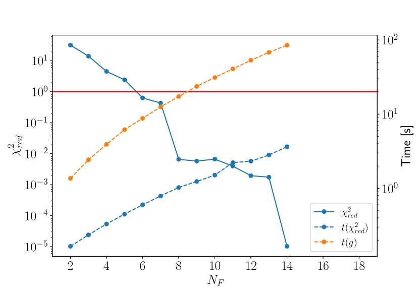
Figure 1: Reduced $\chi^{2}_{red}$ value of the finite-nucleus model as a function of $N_{F}$ for the Woods-Saxon potential. The dashed lines represent the execution time of the $\chi^{2}_{red}$ function and the computation time of the Woods-Saxon FIM.

Table 1: The data set consisting of the charge radii, $r_{ch}$, and single neutron, $\epsilon_{n}$, and proton, $\epsilon_{p}$, energies for occupied states. The single-particle energies are computed using the Woods-Saxon potential as determined in Ref. [30].

Nucleus	$r_{ch}$ (fm)
4He	1.65
16O	2.41
40Ca	3.29
	$\epsilon_{n}$ (MeV)
	$1s_{1/2}$	$1p_{3/2}$	$1p_{1/2}$	$2s_{1/2}$	$1d_{5/2}$	$1d_{3/2}$
4He	$-$25.30
16O	$-$43.20	$-$24.68	$-$19.04
40Ca	$-$53.34	$-$39.40	$-$35.40	$-$24.95	$-$18.51	$-$17.42
	$\epsilon_{p}$ (MeV)
	$1s_{1/2}$	$1p_{3/2}$	$1p_{1/2}$	$2s_{1/2}$	$1d_{5/2}$	$1d_{3/2}$
4He	$-$24.95
16O	$-$40.08	$-$22.39	$-$18.36
40Ca	$-$45.80	$-$33.08	$-$30.32	$-$19.53	$-$14.96	$-$13.23

Figure 2: Relative error of the different FIM components, color-coded as a function of $N_{F}$ and numerical derivative step $h$. The relative error compares the AD-derived FIM estimate, $g_{\mu\nu}^{(A)}$, to the numerical estimate $g_{\mu\nu}^{(N)}$. On the bottom-right panel, the sum of all relative errors, $\sum_{\mu\nu}R(g_{\mu\nu})$, is plotted.

We analyze the statistical properties of the RMF procedure on charge-radius, $r_{ch}$, and single-particle energy data. To this end, we choose a set of doubly magic nuclei: ⁴He, ¹⁶O, and ⁴⁰Ca. Since the parameter space consists of 12 parameters and only three nuclei, the chosen data set consists of their charge-radii and the single-particle energies of protons and neutrons for occupied states, computed using the values of Ref. [30]. For statistical analyses, these parameter values were taken as the best-fitting values for the Woods-Saxon potential.

Using charge radii and the energies of the occupied single-particle states results in 23 data points, ensuring enough degrees of freedom for a twelve-parameter model. A further simplification comes from the fact that the proton and neutron numbers are the same in all three nuclei, excluding the parameter $\kappa$ and thereby reducing the parameter space to 11 dimensions. We compute the charge-radius, $r_{ch}$, from the root-mean-square radius, $\langle r^{2}\rangle$, (as in, e.g., [26]) using the proton density distribution, as $r_{ch}=\sqrt{\langle r^{2}\rangle+0.64}$. A homoscedastic error of $0.1\,\mathrm{fm}$ and $0.1\,\mathrm{MeV}$ has been chosen arbitrarily since the data set consists of the model evaluation and not of spectral measurements. The difference in charge radius and single-particle energy values is smaller than the chosen error.

The corresponding reduced $\chi^{2}_{red}$ value of the finite-nucleus model as a function of $N_{F}$ for the Woods-Saxon potential is shown in Fig. 1. The choice of a different error would only shift the $\chi^{2}_{red}$ curve upwards or downwards. The figure also shows the execution time as a function of the maximal total quantum number $N_{F}$, displayed as a dashed line. The simple relation $\chi^{2}_{red}\approx 1$ should hold to minimize the impact of overfitting and underfitting. The model accomplishes this near $N_{F}\approx 5$. Since the execution time of the $\chi^{2}_{red}$ function rises progressively with a larger $N_{F}$, the value of the $N_{F}$ parameter is set to 5 for statistical analyses. The execution time for the FIM matrix for this model shows similar behavior. The chosen data set is shown in Table 1 and is computed using a $N_{F}=15$, which is set outside the examined $N_{F}$ range in Fig. 1 in order to avoid the artificial $\chi^{2}=0$ data point. The value of $N_{F}$ is chosen to be large enough so that the values of all computed parameters differ by less than $10\%$ of the adopted value for the homoscedastic error between neighboring values of $N_{F}$.

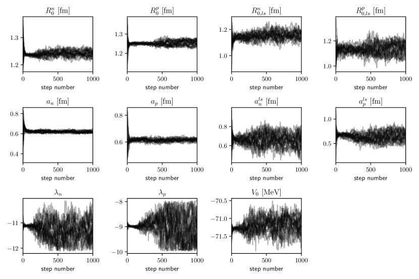
Figure 3: Values of the individual Markov chains of the MCMC sampling as a function of the MCMC step.

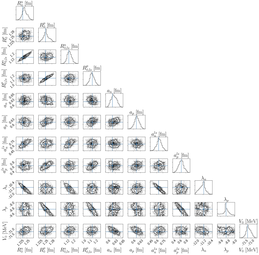
Figure 4: MCMC-derived sampling of the Woods-Saxon potential shown as two-dimensional sections of the parameter space.

Table 2: Results of the Woods-Saxon potential fitting using the FIM-based techniques and the MCMC method for the charge radius and single-particle energy data set given in Table 1. In the last two columns shown are $Z$ scores defined in Eq. (35).

Parameter	Ref. [30]	$\sigma_{\textnormal{MCMC}}$	$\sigma_{\textnormal{FIM}}$	MCMC interval	Confidence	$|Z(\sigma_{\textnormal{MCMC}})|$	$|Z(\sigma_{\textnormal{FIM}})|$
$R_{0}^{n}$ (fm)	1.2334	0.0095	0.0112	$1.24\pm 0.01$	[ 1.23, 1.25 ]	0.79	0.66
$R_{0}^{p}$ (fm)	1.2496	0.0108	0.0168	$1.25\pm 0.01$	[ 1.24, 1.26 ]	0.28	0.18
$R_{0,ls}^{n}$ (fm)	1.1443	0.0273	0.0320	$1.15\pm 0.03$	[ 1.13, 1.18 ]	0.27	0.23
$R_{0,ls}^{p}$ (fm)	1.1401	0.0389	0.0563	$1.14\pm 0.04$	[ 1.10, 1.18 ]	0.11	0.07
$a_{n}$ (fm)	0.6150	0.0097	0.0098	$0.62\pm 0.01$	[ 0.61, 0.63 ]	0.56	0.55
$a_{p}$ (fm)	0.6124	0.0107	0.0108	$0.61\pm 0.01$	[ 0.60, 0.63 ]	0.20	0.20
$a^{ls}_{n}$ (fm)	0.6476	0.0601	0.0746	$0.66\pm 0.06$	[ 0.60, 0.72 ]	0.23	0.18
$a^{ls}_{p}$ (fm)	0.6469	0.0848	0.1271	$0.64\pm 0.08$	[ 0.56, 0.72 ]	0.05	0.03
$\lambda_{n}$	$-$11.1175	0.3391	0.4167	$-11.3\pm 0.3$	[ $-$11.65, -10.98 ]	0.49	0.39
$\lambda_{p}$	$-$8.9698	0.4287	0.7025	$-9.0\pm 0.4$	[ $-$9.47, $-$8.61 ]	0.07	0.04
$V_{0}$ (MeV)	$-$71.2800	0.1941	0.2228	$-71.2\pm 0.2$	[ $-$71.37, $-$70.99 ]	0.45	0.39
$\kappa$	0.4616

IV Results

We apply the finite nucleus procedure to compute parameter uncertainties for the Woods-Saxon potential. We estimate errors of the model parameters obtained by computing the diagonal elements of the FIM, $\sigma_{\textnormal{FIM}}$, as presented in Table 2. Below we compare the values of the FIM components computed using AD and those computed using numerical differentiation. We also compare the FIM-derived error estimates to those of the MCMC technique.

The numerical differentiation is compared to the one that employs a symmetric differentiation step $h$. Figure 2 shows the relative error, $R$, for the different components of the FIM, which is computed as

$$R(g_{\mu\nu})=\left|\frac{g_{\mu\nu}^{(A)}-g_{\mu\nu}^{(N)}}{g_{\mu\nu}^{(A)}}\right|\;.$$ (34)

Here, $g_{\mu\nu}^{(A)}$ is our AD-derived FIM estimate of the $\mu\nu$ matrix component of the FIM, and $g_{\mu\nu}^{(N)}$ is the numerical estimate computed with a differentiation step $h$. In Fig. 2 we show these relative errors computed for different values of $h$ and $N_{F}$. For very small values of $h<10^{-7}$ the numerical errors due to floating point precision accumulate, while for $h>10^{-2}$ the finite difference approximation tends to break down. This behavior is observed for all $N_{F}$, and the relative error values do not depend strongly on $N_{F}$. To assess the overall worst-case error scenario, we compute the sum of all relative errors, $\sum_{\mu\nu}R(g_{\mu\nu})$. This quantity is shown in the bottom right panel of Fig. 2, and suggests that the optimal $h$ is consistently $h\approx 10^{-4}$ for the entire range of $N_{F}$. We conclude that the AD implementation provides accurate estimates of the FIM and that any discrepancy to the numerical derivative can be attributed to the inherent issues of numerical derivatives.

We use the MCMC technique to sample the $\chi^{2}$ posterior distribution, as implemented in the package EMCEE [31]. We use samples of 24 Markov chains of length 1000. The number of initialized chains is chosen to fulfill the MCMC requirement that the number of Markov chain walkers be greater than the number of dimensions of the parameter space. In Fig. 3 we plot the values of the MCMC samples of the parameter space as a function of the step in the Markov chain in which they are produced. We see that the values stabilize after $\approx 50$ initial steps, indicating the expected burn-in phase for the MCMC method [31]. The sampled data points corresponding to the initial 50 steps are excluded from further analysis.

In Fig. 4 we show both the two-dimensional and one-dimensional marginal distributions of the MCMC samples in the parameter space. The blue lines show the value expected from the literature, which is well aligned with the distribution of the MCMC samples in all panels in Fig. 4. The error estimates computed with MCMC sampling are listed alongside the FIM-based technique in Table 2. The medians and the $1\sigma$ confidence interval derived with the MCMC sampling are well aligned with the estimates in Ref. [30]. To assess the degree of statistical differences between the parameters estimated in Ref. [30], $p^{\mu}_{0}$, and the MCMC-based best-fitting parameter values of our data set, $p^{\mu}$, we list in the last two columns of Table 2 the $Z$ scores, defined by

$$Z^{\mu}(\sigma)=\frac{p^{\mu}_{0}-p^{\mu}}{\sigma}\;.$$ (35)

We find that the differences are generally not statistically significant (i.e., they are less than $1\sigma$), regardless of whether $\sigma_{\textnormal{FIM}}$ or $\sigma_{\textnormal{MCMC}}$ is considered. The FIM method is based on the assumption of the Gaussianity of errors, while the MCMC algorithm is not constrained in that way. Using longer MCMC chains would remove the remaining numerical differences between $\sigma_{\textnormal{FIM}}$ and $\sigma_{\textnormal{MCMC}}$ in Table 2. Choosing to compute error estimates via MCMC sampling over FIM would only be useful if there is a need to analyze the impact of non-Gaussian errors.

In contrast to simply considering the diagonal elements of the FIM inverse, by reliably computing the FIM with the aid of AD, one can perform error analysis without invoking the time-consuming sampling of the parameter space. The resulting estimates, $\sigma_{\textnormal{FIM}}$, are in agreement with the MCMC estimates, $\sigma_{\textnormal{MCMC}}$, as shown in Table 2.

V Conclusion

Uncertainties related to parameter estimation for nuclear EDFs have recently become a topic under rigorous investigations. By extending our previous study of [22], in which methods of information geometry was applied to EDFs in the case of infinite nuclear matter, in this work we have presented a statistical analysis of a simple procedure for determining the RMF binding energies for a set of doubly-magic nuclei with the Woods-Saxon potential. We have compared error estimates between the faster procedure that employs the FIM and the numerically more challenging Bayesian MCMC method. Even in the complex case of finite nuclei, EDF parameter uncertainties can be reliably estimated by using the FIM combined with algorithmic differentiation. The proposed approach to error analysis has the advantage of avoiding the time-consuming sampling of the parameter space, which would otherwise be required in Bayesian statistical techniques.

In our next step, by using the optimized Woods-Saxon potential resulting from the present analysis, we will apply nuclear structure codes to give error estimates for the point-coupling models, such as the universal EDF DD-PC1, for a realistic study of finite nuclei. Work along this line is in progress, and will be reported elsewhere.