$QFactor$: A Domain-Specific Optimizer for Quantum Circuit Instantiation

Abstract

We introduce a domain-specific algorithm for numerical optimization operations used by quantum circuit instantiation, synthesis, and compilation methods. $QFactor\$uses a tensor network formulation together with analytic methods and an iterative local optimization algorithm to reduce the number of problem parameters. Besides tailoring the optimization process, the formulation is amenable to portable parallelization across CPU and GPU architectures, which is usually challenging in general purpose optimizers (GPO). Compared with several GPOs, our algorithm achieves exponential memory and performance savings with similar optimization success rates. While GPOs can handle directly circuits of up to six qubits, $QFactor\$can process circuits with more than 12 qubits. Within the BQSKit optimization framework, we enable optimizations of 100+ qubit circuits using gate deletion algorithms to scale out linearly with the hardware resources allocated for compilation in GPU environments.

I Introduction

Quantum compilers have many purposes, but none are more critical than reducing circuit gate count. This goal is especially true in the Noisy Intermediate-Scale Quantum (NISQ) era, where each gate can have a high cost in additional error rates. Compilation approaches that use numerical optimization, commonly named instantiation-based methods, are heavily used in quantum program development and optimization. Hybrid quantum-classical algorithmic workflows such as VQE [1] and QAOA [2] repeatedly instantiate parameterized quantum circuit (PQC) ansatz, which have gates represented in their parameterized form, e.g., $R_{x}(\theta)$. Circuit instantiation is directly supported by popular compilation infrastructures such as IBM Qiskit [3], Google Cirq [4], or Tket [5]. Instantiation is also an important step in circuit synthesis tools such as BQSKit [6, 7, 8, 9], NACL [10], Squander [11, 12], and CPFlow [13].

Quantum compilation and synthesis algorithms that utilize numerical optimizers to perform instantiation follow a simple paradigm. First, they will propose a candidate parameterized circuit template and, second, use numerical instantiation to ”best” fit the circuit parameters to the target. One can find a solution by repeating this process as often as necessary. The scalability of the underlying general-purpose numerical optimizer (GPO) limits the scalability of this compilation strategy. This limitation, in turn, limits the number of qubits and gates that instantiation-based methods can directly handle.

This paper makes the following contributions:

• We introduce Quantum Fast Circuit Optimizer ($QFactor$), a domain-specific optimizer for quantum circuit instantiation, usable in multiple custom or generic compilation workflows, designed to improve their scalability and efficacy.

• We enable optimization approaches based on gate deletion heuristics to scale out when running in hybrid (CPU+GPU) distributed memory environments.

• We provide valuable feedback about the strategy to architect instantiation-based compilation workflows able to handle huge circuits.

The main idea behind $QFactor\$is based on lessons learned from machine learning algorithms that heavily use tensor network formulations, combined with our experience developing scalable quantum synthesis infrastructures. Tensor network algorithms have been also extensively used to simulate quantum circuits [14, 15, 16, 17, 18]. All existing instantiation-based synthesis approaches [6, 7, 8, 9, 10, 11, 12, 13, 19] use general-purpose optimizers and parameterized gate representations. For example, the parameterization for a rotation is:

$$R_{Y}(\theta)=e^{-i\theta Y/2}=\begin{pmatrix}\cos{\frac{\theta}{2}}&-\sin{\frac{\theta}{2}}\\ \sin{\frac{\theta}{2}}&\cos{\frac{\theta}{2}}\end{pmatrix}$$ (1)

In contrast, $QFactor\$uses a tensor network formulation, which does not require explicit parameterization, enabling the algorithm to work at the unitary rather than the parameter level. This perspective change drastically reduces the total number of optimized parameters compared to GPOs, because each gate may have many parameters but only one unitary.

We provide a CPU-based implementation written in Rust, together with a Python implementation written using JAX [20]. The Rust implementation is serial, while the Python/JAX implementation benefits from auto-parallelization. For validation we use a suite of algorithms whose implementation ranges from five to 400 qubits, with a total gate count as high as $\approx 170,000$ gates, as shown in Table III.

We first evaluate the instantiation performance of $QFactor\$against Ceres [21] and LBFGS [22, 23, 24]. The GPO’s have good performance for circuits up to 6-7 qubits, while $QFactor\$can process circuits with more than 12 qubits. Best performance is achieved on GPU based systems, which outperform CPUs by 4$\times$ in the bigger circuits. Scalability is problem dependent, and we conjecture that the new formulation is limited only by GPU memory size. The success rate of $QFactor\$is similar to that of GPOs for circuits evaluated.

To leverage $QFactor$’s advantages in circuit instantiation, we incorporated it into BQSKit‘s [6] gate deletion based optimization [9] pipeline, which can handle circuits with 100s of qubits. To ensure scalability for large qubit and depth count circuits, BQSKit partitions these into smaller panels which are then directly optimized. When comparing configurations of this approach using GPOs or $QFactor$, $QFactor\$improves the optimized circuit quality by enabling the usage of bigger partitions, thus reducing U3 and CNOT gate count, in some cases, by more than $30\%$ . Furthermore, $QFactor\$appears to scale linearly with resources on GPU based systems, while all the other CPU based implementations suffer from load balancing problems.

Given their efficacy in optimizing circuits, infrastructures similar to BQSKit are very attractive for NISQ systems, where gate count and circuit depth affect fidelity. The capability to directly instantiate bigger circuits enables us to draw very useful conclusions to guide the architecture of such hierarchical transformation approaches that combine partitioning and instantiation. The memory footprint of instantiation scales exponentially with qubits, and it is therefore limited by the memory capacity of a system. At the high-end qubit count (e.g. IBM Osprey with 433 qubits) a legitimate question is whether we should strive to develop even more scalable direct instantiation methods or have we already reached diminishing returns. Our experimental data empirically indicates that the latter might be the case: benefits seem to saturate when using partitions with more than 8-9.

Besides the benefits showcased in this paper, $QFactor\$is definitely very useful and enables other optimization approaches. We have formulated the prototype algorithm in Python circa 2021 and have since used it in optimization of convolutional neural networks and unitary compilation [25], state preparation [26], learning fast scramblers [27] and in conjunction with variable ansatz techniques [28]. Furthermore, as the performance gap between GPUs and CPUs is likely to increase, the availability of a scalable domain specific optimizer for instantiation bodes well for the future of hierarchical synthesis approaches.

The organization of this paper is as follows. Section II introduces the background concepts. Section III provides a detailed description of the algorithm, while Section IV covers all the implementation details. The evaluation methods and results are presented in Section V, and the discussion of the results is presented in Section VI. Finally, Section VII provides the conclusion of the paper.

II Background

Parameterized Circuit Instantiation: Instantiation is the process of finding the parameters for a circuit’s gates that make it to most closely implement a target unitary. For a $n$-qubit parameterized quantum circuit $C:\mathbb{R}^{k}\mapsto U(N)$ and a target unitary $V\in U(N)$, where $N=2^{n}$, solve for

$$\operatorname*{argmax}_{\alpha}{|\mathrm{Tr}(V^{\dagger}C(\alpha))|}$$

where $k$ is the number of gate parameters in the circuit, and $U(N)$ is the set of all $N\times N$ unitary matrices. This definition is very general and considers the parameterized circuit as a parameterized unitary operator, see Figure 1. The $|\mathrm{Tr}(V^{\dagger}C(\alpha))|$ component measures the Hilbert-Schmidt inner product, which physically represents the overlap between the target unitary and the circuit’s operator. The maximum value this can have is equal to $N$, the dimension of the matrix, and this occurs when $C(\alpha)$, the unitary of the circuit with gate parameters $\alpha$, is equivalent to $V$ the target unitary up to a global phase.

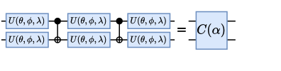
Figure 1: This is an example of a parameterized quantum circuit on the left. It is composed of three-parameter universal single-qubit rotations and two-qubit CNOT gates. For direct simulation, we can represent the circuit by its unitary operator shown on the right, which is calculated by tensor contraction of all of its gates. Furthermore, we can represent parameterized circuits by a parameterized unitary $C(\alpha)$, which can be instantiated to some other unitary $V$ by solving for the parameters $\alpha$ that maximize the overlap of $C(\alpha)$ and $V$. This can be accomplished with analytic methods in specific cases and gradient descent or other numerical methods in the general case.

Techniques that perform instantiation are ubiquitously deployed in quantum compiler toolchains from industry and academia. The most common form is the KAK [29] decomposition, which uses analytic methods to produce the two-qubit circuit that implements any two-qubit unitary. KAK uses a native gate set composed of single-qubit rotations and CNOT gates.

Recently, bottom-up approaches to quantum synthesis have been successful through numerical instantiation [8, 7, 10, 11, 12, 30]. When compared to KAK, they handle circuits of more than two qubits, roughly up to 6-7 qubits, albeit with large runtime overhead. When compared against commercial compilers such as Qiskit, Cirq, and Tket, direct synthesis techniques have been shown to provide higher quality circuits. Rather than fixed mathematical identities, these techniques employ a numerical optimizer to closely approximate a solution to the instantiation problem. This is done by minimizing a cost function, often the unitary error or distance between the circuit’s unitary and a target unitary. This is given by the following formula using the same notation as before.

$$\Delta(C(\alpha),V)=1-\frac{|\mathrm{Tr}(V^{\dagger}C(\alpha))|}{N}$$

Other variations of this distance function include:

$$\Delta_{f}(C(\alpha),V)=1-\frac{\mathrm{Re}(\mathrm{Tr}(V^{\dagger}C(\alpha)))}{N}$$

and

$$\Delta_{p}(C(\alpha),V)=\sqrt{1-\frac{|\mathrm{Tr}(V^{\dagger}C(\alpha))|^{2}}{N^{2}}}$$

All three cost functions have a range of $[0,1]$, and as they approach zero, the circuit’s unitary approaches $V$.

Numerical Optimization in Instantiation: Synthesis tools can use either derivative-free or gradient-based general purpose optimizers when the problem formulation allows it. For example, Davis et al [8] discuss derivative-free (CMA-ES, COBYLA, and BOBYQA) and gradient-based optimization (BFGS and Levenberg-Marquardt) for a synthesis algorithm that uses $U3(\theta,\phi,\lambda)$ parameterized single-qubit gates. They report that the Ces [21] implementation of Levenberg-Marquardt with gradients provides up to $100\times$ execution time improvements when compared to the implementation of COBYLA provided in scipy, with better scaling as the number of variables increases. Many quantum compiling frameworks utilize gradient-descent optimizers such as L-BFGS [23, 24] and least-squares optimizers such as Levenberg Marquardt [31] for certain compilation objectives.

Lavrijsen et al [32] provide a thorough study of optimizers appropriate for hybrid quantum-classical variational algorithms, which perform instantiation in their classical step. They evaluate (hybrid) mesh algorithms (ImFil [33], NOMAD [34]); local fit (SnobFit [35]); and trust region algorithms (PyBobyqua [36, 37]).

Overall, all these instantiation studies agree that the scalability of the numerical optimizer with circuit size is the biggest bottleneck. Improving it can only lead to shorter time to solution with better quality results. Based on our previous experiences and literature recommendations, in this study we choose to compare against the gradient-descent L-BFGS [24, 23] optimizer and the Levenberg-Marquardt [31] least-squares optimizer.

Partitioning and Resynthesis: Approaches that numerically optimize the parameters of a circuit by simulating it encounter exponential-scaling issues with the increase in qubits and circuit depth. As a result, direct methods are often limited to low dimensionality problems with few qubits and shallow circuits. Hierarchical approaches can overcome these scaling issues. These methods will group closely located gates into fixed-width blocks and then resynthesize or transform them with numerical optimization-based strategies. This process is illustrated in Figure 2.

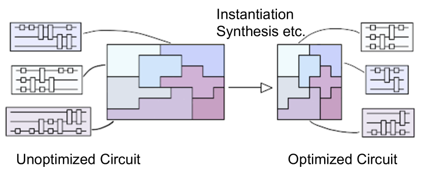
Figure 2: Hierarchical synthesis or instantiation based circuit optimization. Both partitioning strategy and quality of numerical optimization determine performance and final output quality.

Approaches that follow this similar partitioning-driven flow, such as QGO [38] and BQSKit [6], have been shown to scale to 1000s of qubits, but could only use three qubit partitions due to slow numerical optimization. Their behavior is likely influenced by the block size for both result quality and completion time. The number of qubits chosen per block makes an impact, because more qubits are likely to capture more domain-level physical interactions, leading to better optimization opportunities. On the other hand, larger blocks require more memory since they need to be represented by exponentially larger matrices, and they require more processing time due to the increase in the number of parameters. Improving instantiation is likely to lead to improved compilation performance, as well as output circuit quality.

III Algorithm

$QFactor\$simplifies the circuit’s parameter complexity by directly updating (possibly multi-qubit) unitary gates without parameterizing them internally. The optimization is done by performing an iterative sweep through all the gates. During every step, $QFactor\$locally optimizes each gate. This ability to treat each gate as a unitary without parameterization during optimization sets $QFactor\$apart from other general-purpose optimizers and makes it particularly effective.

Given $2^{n}\times 2^{n}$ unitary $V$, $QFactor\$finds unitaries $u_{1},\ldots,u_{p}$ such that the Froebenius norm between $V$ and unitary $U\equiv u_{1}\cdot\ldots\cdot u_{p}$ is minimized.

$$||U-V||^{2}=2^{n+1}\left(1-\frac{1}{2^{n}}\mathrm{Re}\mathrm{Tr}(V^{\dagger}U)\right)\ .$$ (2)

Note that the “$\cdot$” in $u_{1}\cdot u_{2}$ represents tensor contraction, as shown in Fig. 3(a). Formally, the operation is properly defined only when information on all qubits participating in any $u_{k}$ is given. We drop that information for simplicity. Since all gates $u_{k}$’s enter Eq. (2) linearly, $\mathrm{Tr}(V^{\dagger}U)$ can be written as $\mathrm{Tr}(\mathcal{E}u_{k})$, where $\mathcal{E}$, so-called environment matrix [39], does not depend on $u_{k}$, see Fig. 3(b) and (c). This fact is used in optimization over $u_{k}$’s, as described later in Section III-A.

Figure 3: Tensor network calculations used in $QFactor$. (a) An example of a tensor contraction. Three-qubit gate $u_{1}$ is contracted with two-qubit gate $u_{2}$ to form gate $U=u_{1}\cdot u_{2}$. (b) Four-qubit example of a cost function in Eq. (2) (up to constant factors). Here, $U=u_{1}\cdot u_{2}\cdot u_{3}$. The value of $\mathrm{Tr}(V^{\dagger}U)$ is represented as a tensor network. Bent qubit line represents partial trace. $\mathrm{Tr}(V^{\dagger}U)$ can be written as $\mathrm{Tr}(\mathcal{E}u_{2})$, where the transpose of environment matrix $\mathcal{E}$ is defined in (c). Tensor $T$ is constructed in the process of computing environment matrix $\mathcal{E}$, $T=u_{3}\cdot V^{\dagger}\cdot u_{1}$.

The problem is thus to find

$$\operatorname*{argmin}_{\{u_{k}\}}||u_{1}\cdot\ldots\cdot u_{p}-V||$$ (3)

or equivalently

$$\operatorname*{argmax}_{\{u_{k}\}}\mathrm{Re}\mathrm{Tr}(V^{\dagger}u_{1}\cdot\ldots\cdot u_{p})\ .$$ (4)

III-A Optimization Algorithm

The algorithm uses the fact that the local optimization problem

$$\operatorname*{argmax}_{u\mathrm{-unitary}}\mathrm{Re}\mathrm{Tr}(\mathcal{E}u)$$ (5)

can be solved exactly for any arbitrary environment matrix $\mathcal{E}$. As shown in Alg. 1, $QFactor\$iteratively calculates the environment matrix for each gate and optimizes its unitary, thus gradually improving the implementation of the circuit.

$QFactor\$updates unitaries $u_{k}$ sequentially and individually. It starts with $u_{1}$ and proceeds to the right, updating $u_{p}$ in the final step. It then updates the unitaries in the opposite direction. This sequence of updates forms one iteration of the algorithm and is called TwoSidedSweep. Every individual update of a given $u_{k}$ is done by calculating it’s enviorment, see Fig 3(c) and then using the SVD update described and proved in Section III-A1. This update is referenced as OptimizeGate in Alg. 1.

Naively, one needs to recalculate each environment matrix for each of the gates after a gate update. $QFactor\$has an optimization that reduces both the memory and runtime complexity of these calculations by reusing previous calculations. It represents $V^{\dagger}U$ as a tensor, which we call the circuit tensor. $QFactor\$sweeps over the gates with a “peephole” by applying the gates or their inverse to the left or to the right of the tensor according to the algorithm phase. Applying a gate is simply contracting the circuit tensor with the gate tensor, as seen in Fig. 3(a). Applying the inverse of a gate removes it from the tensor, and by tracing all the other legs of the circuit tensor we create the environment or ”peephole”, as can be seen in Fig 3(c). The initial creation of the circuit tensor and the sweeping procedure can be seen in Alg. 1 at InitCircuitTensor and TwoSidedSweep respectively. The tracing procedure is referenced as CalcEnvMat in Alg. 1.

The $QFactor\$algorithm is designed such that every iteration does not increase the cost function; rather, it can only decrease or reach a plateau. To facilitate termination, the algorithm employs a mechanism composed of multiple criteria. The primary criterion for termination is achieving the goal of instantiating the parameterized circuits to the target unitary within a given tolerance. Additionally, the algorithm terminates when it detects that it has reached a plateau or when it has completed a maximum number of iterations. For a detailed explanation of the hyperparameters that influence the algorithm behavior, please refer to Section III-A2.

III-A1 Local Optimality Proof

Let us write singular value decomposition of $\mathcal{E}$ as $\mathcal{E}=XDY^{\dagger}$, with unitary $X$, $Y$ and diagonal, real, non-negative $D$.

We have

$$\mathrm{Re}\mathrm{Tr}(\mathcal{E}u) =\mathrm{Re}\mathrm{Tr}(XDY^{\dagger}u)$$

$$=\mathrm{Re}\mathrm{Tr}(DY^{\dagger}uX)=\mathrm{Re}\mathrm{Tr}(DW)$$ (6)

for some unitary $W$.

Finally,

$$\mathrm{Re}\mathrm{Tr}(DW)=\sum_{j}D_{jj}\mathrm{Re}W_{jj}\leq\sum_{j}D_{jj}\ .$$ (7)

$\sum_{j}D_{jj}\mathrm{Re}W_{jj}$ is maximized by setting all $W_{jj}=1$. $W$ is unitary, so the maximum is achieved at $W=\mathrm{I}$, the identity matrix. This means that the unitary that solves (5) is given by

$$u_{\textrm{new}}=YX^{\dagger}\ .$$ (8)

III-A2 $QFactor$’s Hyperparameters

$QFactor\$has the following hyperparameters that control the termination conditions of the algorithm, and update policy and randomization:

• dist_tol - When the distance between the target unitary to the current circuit reaches dist_tol, the algorithm stops. We calculate the distance as $||u_{1}\cdot\ldots\cdot u_{k}-V||$.

• diff_tol_a and diff_tol_r - The algorithm will terminate if $|c_{i}|-|c_{i-1}|\leq\textit{diff\_tol\_a}+\textit{diff\_tol\_r}*|c_{i}|$ where $c_{j}$ is the cost function value after iteration $j$.

• long_diff_count and long_diff_r - Control the long plateau detection mechanism. The algorithm will terminate if over the course of long_diff_r iterations, the cost function did not decrease by long_diff_r, i.e. the condition

  $$|c_{i}|-|c_{i-\textit{long\_diff\_count}}|\leq\textit{long\_diff\_r}*|c_{i-\textit{long\_diff\_count}}|$$

  must be met to continue the optimization. Here $c_{j}$ is the cost function value after iteration $j$.

• min_iter - Sets the minimum amount of iterations for $QFactor\$to complete before stopping.

• max_iter - Sets the maximum amount of iterations. The algorithm will always stop when it reaches this limit.

• reset_iter - In order to conserve memory, the algorithm (effectively) performs operations that should evaluate to identity. For example, it applies gate $u$ to compute environment and then applies $u^{\dagger}$ at a later step. This builds rounding error over many iterations, which can be observed in practice. Thus, for numerical stability, we reset the circuit tensor every reset_iter iterations. Choosing small values for this configuration parameter has a performance impact. From our experience setting it to 40, has minimal performance impact and provides a wide safety margin.

• multistarts and seed - To overcome the local minimum problem, one can run $QFactor\$with various initial gate unitaries, in the hope that at least one of the runs will lead to a good solution. The initial random unitaries for each gate are controlled by a seed parameter.

• Beta - Is a regularization parameter that controls the retention of the old value in the gate update step. Instead of performing the SVD operation on the environment $\mathcal{E}$, it is done on

  $$(1-\beta)\mathcal{E}+\beta*u^{\dagger}$$

  This parameter is useful in overcoming slow convergence for circuits that have dependency between gates, and the local optimization fails to realize it. At the limits, setting $\beta=0$ corresponds to a “full” update described above, while $\beta=1$ results in no update.

From our experience, here are some good initial hyperparameters values: dist_tol $=10^{-10}$, diff_tol_a $=0$, diff_tol_r $=10^{-5}$, long_diff_count $=100$, long_diff_r $=0.1$, min_iter $=0$, max_iter $=10^{5}$, reset_iter $=40$, multistarts $=8$, $\beta=0$. By modifying the above mentioned hyperparameters, one can easily adjust the tradeoff between result quality and execution time. If one wishes to get results faster, decrease max_iter, increase diff_tol_r and diff_tol_a. Alternately, one might increase $\beta$ or multistarts to find better results with additional execution overhead.

III-A3 Specializing Gates Sets

Besides using general unitaries as the gate set, $QFactor\$can use more specific parameterized gates. For example, one can target a trapped ion quantum computer that has the single qubit gates $GPI(\theta)$ [40] and $R_{z}(\theta)$ and the Mølmer-Sørenson entangling gate $MS(\phi_{1},\phi_{2})$ [41]. In those situations, the SVD approach isn’t viable and we need to directly find $\operatorname*{argmax}_{\theta}\mathrm{Re}\mathrm{Tr}(\mathcal{E}G(\theta))$. This is an easy task, as we can analytically calculate a formula that gives the maximum for a given environment. For example, let’s examine the calculation needed for optimizing the $R_{z}$ gate. The unitary of $R_{z}(\theta)$ is given by

$$Rz(\theta)=\left(\begin{array}[]{cc}1&0\\ 0&e^{i\theta}\end{array}\right)$$

Hence, we need to find $\theta$ that maximizes

$$\mathrm{Re}\mathrm{Tr}(\mathcal{E}Rz(\theta)) =\mathrm{Re}\mathrm{Tr}\left(\left(\begin{array}[]{cc}\mathcal{E}_{0,0}&\mathcal{E}_{0,1}\\ \mathcal{E}_{1,0}&\mathcal{E}_{1,1}\end{array}\right)*\left(\begin{array}[]{cc}1&0\\ 0&e^{i\theta}\end{array}\right)\right)$$

$$=-\mathrm{Re}(\mathcal{E}_{1,1})\cos{\theta}+\mathrm{Img}(\mathcal{E}_{1,1})\sin{\theta}$$

When $\mathrm{Re}(\mathcal{E}_{1,1})>0$ and $\mathrm{Img}(\mathcal{E}_{1,1})\neq 0$ the maximum is achieved by:

$$\theta_{\textrm{new}}=\arctan{\frac{\mathrm{Re}(\mathcal{E}_{1,1})}{\mathrm{Img}(\mathcal{E}_{1,1})}}$$

Algorithm 1 $QFactor$

function InitCircuitTensor(target unitary, unitaries, locations)

     $ct\leftarrow reshaped\leavevmode\nobreak\ target\leavevmode\nobreak\ unitary$

     for $(u,l)\in(unitaries,locations)$ do

         $ct\leftarrow\textsc{ApplyRight}(ct,u,l,inverse=False)$

     end for

     return $ct$

end function

function TwoSidedSweep(circuit tensor, unitaries, locations, gates)

     $ct\leftarrow\text{circuit tensor}$

     $newUs$ $\leftarrow$ empty list

     for $(u,l,g)\in reversed(unitaries,locations,gates)$ do

         $ct\leftarrow\textsc{ApplyRight}(ct,u,l,inverse=True)$

         $env\leftarrow\textsc{CalcEnvMat}(ct,l)$

         $u_{opt}\leftarrow\textsc{OptimizeGate}(g,env)$

         $newUs$ $\leftarrow$ PrependtoList($newUs$, $u_{opt}$)

         $ct\leftarrow\textsc{ApplyLeft}(ct,u_{opt},l,inverse=False)$

     end for

     $finalUs$ $\leftarrow$ empty list

     for $(u,l,g)\in(newUs,locations,gates)$ do

         $ct\leftarrow\textsc{ApplyLeft}(ct,u,l,inverse=True)$

         $env\leftarrow\textsc{CalcEnvMat}(ct,l)$

         $u_{opt}\leftarrow\textsc{OptimizeGate}(g,env)$

         $finalUs$ $\leftarrow$ AppendtoList($finalUs$, $u_{opt}$)

         $ct\leftarrow\textsc{ApplyRight}(ct,u_{opt},l,inverse=False)$

     end for

     return $ct$, $finalUs$

end function

function Qfactor(target unitary, initial unitaries, locations, gates, termination conditions)

     $ct\leftarrow$ InitCircuitTensor(target unitary, initial unitaries, locations)

     $unitaries\leftarrow$ initial unitaries

     repeat

         $ct$, $unitaries\leftarrow$ TwoSidedSweep($ct$, $unitaries$, locations, gates)

         calculate cost function and detect a plateau

     until termination conditions not met

     return $unitaries$

end function

IV $QFactor\$Implementation

We implemented $QFactor\$as a standalone optimizer in Python (https://github.com/BQSKit/qfactor) and Rust (https://github.com/BQSKit/bqskitrs). These are serial CPU based implementations. We also provide a parallel version using JAX [20]. All $QFactor$’s implementations have also been incorporated into the BQSKit compilation infrastructure at https://github.com/BQSKit/bqskit.

IV-A Migrating to GPU using JAX

GPUs have been shown to significantly outperform CPUs for tensor network formulations, due to their ability to execute more operations in parallel. We have ported the $QFactor\$Python implementation to a GPU implementation using the JAX framework [20]. This allows us to seamlessly parallelize the instantiation across different multistarts and JIT our code to better utilize the GPU, while still working at a high level of representation in Python. To fully utilize the GPU, even when using small partitions that don’t saturate the GPU, we use NVIDIA’s MPS [42], which enables different processes to share GPU resources and dynamically allocate them according to the changing load of each process.

In contrast to the CPU implementation, where the instantiation using different starting conditions is done in sequence, on the GPU all the multistarts are done in parallel - this raises the question of when should the optimization be terminated. Of course, if one of the multistarts was able to converge to the correct solution, we can stop and return that result. The tricky case is termination by plateau detection. As explained in Section III, $QFactor\$can get stuck in local minima, so the heuristic of plateau detection needs to take into account the parallel multistarts and terminate only if all of them have hit a plateau.

V Evaluation

We evaluate $QFactor\$on a set of benchmarks that represent real circuits ranging from four to 400 qubits and containing up to $\approx 200,000$ gates, as illustrated in Table III. We use circuits that implement classical operations (multiply, add) [43], the HHL, Shor [44] and Grover algorithms [45], variational algorithms (VQE and QAOA) [2, 46], Quantum Phase Estimation circuits, Heisenberg and Hubbard models [47, 48], and Transverse Field Ising Model circuits [49, 50].

After gathering all the benchmarks, we standardized them to the U3 and CNOT gate-set. We accomplish that by using the Qiskit [3] compiler with no optimizations (O0). The standardized benchmarks can be found in the qce23 benchmark repository on GitHub [51].

We compare against two leading general-purpose numerical optimizers, which we will refer to as CERES [21] and LBFGS [23, 22, 24]. These are production quality, ubiquitously used optimizers. Furthermore, their hyperparameters have been carefully tuned by Davis et al [8, 52] for instantiation in BQSKit.

We study the performance of each implementation on both CPUs and GPUs, and we benchmark serial execution, single device (CPU or GPU), as well as strong scaling in distributed memory. For strong scaling we use the BQSKit internal runtime support instead of relying on JAX. Also, while JAX can support auto-parallelization for CPU, it’s performance is notoriously bad, also true for our experiments. Therefore we do not evaluate $QFactor\$implemented in JAX on CPUs. Note also that for large circuits that are partitioned, while the workload is embarrassingly parallel, strong scaling behavior is ultimately determined by load balancing.

We first compared the ability to solve instantiations for each optimizer. In these experiments, we assign a time budget to each instantiation request and measure the success rate (defined as finding a solution) on a set of circuits. The results are presented in Section V-A. To evaluate practical usage in circuit transformations, we also assess the quality of each optimizer based on the U3 and CNOT gate reduction in circuits produced by a new BQSKit hierarchical gate deletion pass implemented using $QFactor$. This workflow is discussed in Section V-B.

In our comparison, we denote the Rust and Python+JAX implementations of $QFactor\$by QF-RUST and QF-JAX respectively. To distinguish parallel CPU runs, we suffixed the instantiator name with ’_P’.

The evaluation shows that when comparing LBFGS against CERES, while the former is slightly slower for serial execution on CPUs, they exhibit similar quality for parallel executions. Therefore, we select CERES for most comparisons, omitting detailed LBFGS results for brevity.

Evaluation Setup: Our evaluation was done on NERSC’s Perlmutter[53] supercomputer, which has two node flavors: hybrid GPU-CPU or pure CPU. Each hybrid node has one AMD EPYC 7763 64-core processor, 256GB DDR4 DRAM, and four NVIDIA A100 40GB GPUs, while each CPU node has two AMD EPYC 7763 64-core processors and 512GB DDR4 DRAM. The CPU-only workloads(CERES, LBFGS, and QFACTOR-RUST) were run on the CPU nodes, while the GPU workload, JAX implementation of $QFactor\$, ran on the GPU nodes. To better utilize the GPUs we setup an NVIDIA MPS server for each GPU on the node, and each $QFactor\$process is instructed to use only a single GPU, leveraging NVIDIA’s CUDA_VISIBLE_DEVICES environment variable.

Each instantiation operation is configured to sample multistarts=32 different starting points. For parallel execution on CPUs we allocate all the cores available. On GPUs we use the entire device, but it requires a more careful decision about the degree of parallelism allowed. Here, there is a tradeoff between partition size and the number of jobs allowed to execute in parallel. Partition “volume” (qubits and gate count) determines both the memory footprint and the amount of hardware resources required for a single job. For a given qubit count, shallow circuits are likely to require fewer execution units than deep circuits. After experimentation, for GPUs we have chosen the set of defaults described in Table I.

The other $QFactor\$hyperparameters used are: dist_tol = $10^{-10}$, diff_tol_a=0, diff_tol_r=$10^{-5}$, long_diff_count=100, long_diff_r=$0.1$, min_iter=0, reset_iter=40, multistarts=32, seed=None, Beta=0.

Partition Size	Workers per GPU
3,4	10
5	8
6	4
7	2
8 and more	1

Table I: Relation between the instantiated partition size and the amount of workers spawned for every GPU

V-A Circuit Instantiation: Runtime and Success Rate

We study $QFactor$’s runtime and success rate efficacy by using it as a standalone instantiation tool on a set of circuits generated by partitioning the input set in Table III into “tiles” ranging from three to 12 qubits. The dataset comprises of 1727 partitions obtained by randomly selecting 10 partitions for every benchmark and partition size. Figures 5 and 5 together with Table II summarize our findings.

Figure 4: Average instantiation time normalized to QF-JAX instantiation time (left-hand side y-axis), together with normalized success rate (right-hand side y-axis), showing the strength of $QFactor\$for larger circuits.

Figure 5: Average instantiation time normalized to QF-JAX instantiation time, in log scale. Lower is faster. While there are some differences in serial execution time between LBFGS and CERES, these wash out in parallel executions (LBFGS_P and CERES_P).

Partition size	Instantiation name
	CERES_P	QF-JAX	QF-RUST_P
3	1.00	0.87	1.00
4	1.00	0.83	1.00
5	1.00	0.78	0.98
6	0.97	0.74	0.86
7	0.93	0.68	0.66
8	0.69	0.58	0.60
9	0.50	0.51	0.53
10	0.30	0.42	0.38
11	0.10	0.27	0.29
12	0.01	0.14	0.16

Table II: Instantiation success rate comparison. $QFactor\$has a better succuss rate in partitions with more than 8 qubits. For the small partitions, the platue detection mechanism in $QFactor\$is the main cause of unsuccessful intantiation.

We give each optimizer a time budget of 10 minutes for circuits with up to 8 qubits and 2 hours for all the rest. We set the distance target $||u_{1}\cdot\ldots\cdot u_{k}-V||$ to $10^{-10}$, as previous studies [8, 54] have shown that this is enough to guarantee good output fidelity when running on NISQ devices, as well as when simulating a perfect QPU. We measure the success rate of each optimizer to find a solution within the time budget.

Figure 5 shows a comparison of the average instantiation time plotted against the left-hand side y-axis and success rate plotted against the right-hand side y-axis. The results indicate clearly that for the high volume circuits, in our data set, for partitions with more than six qubits $QFactor\$outperforms CERES in performance, and for partitions with more than eight qubits $QFactor\$also has a better success rate. At the bigger partition sizes, the GPU implementation of $QFactor\$outperforms the Rust based CPU implementation by an order of magnitude. A detailed comparison of the success rate is given in Table II.

For circuits with fewer than six qubits in our data set, the behavior is more nuanced. For the three qubit circuits, results clearly indicate that CERES offers the best behavior. For the circuits with four to six qubits, the results seem to indicate that CERES is also best, e.g. 4-5 times faster and with a 2%-22% better success rate for five qubit circuits.

However, these results are skewed by the procedure used to generate the benchmarking input set: we draw small “circuits” from partitions of high qubit count circuits associated with proper algorithms, e.g. tfim400. Due to the circuit structure of the algorithms, our sample data set contains mostly circuits with a relatively low volume. For example, the average number of U3s and CNOTs in our sample of five-qubit circuits is 50 and 38 respectively. In contrast, the four-qubit hub4 Hubbard model circuit contains 155 and 180 U3s and CNOTs respectively.

For small volume circuits, CERES indeed does best in terms of success rate and performance. For high volume circuits $QFactor\$offers much better performance, again by orders of magnitude. For example for the hub4 Hubbard model circuit, which uses four qubits and contains 335 gates, $QFactor\$is 5 times faster. The success rates of $QFactor\$and CERES are comparable across all four and five qubit circuits we studied, with slight differences for six qubit circuits. Most of the differences can be attributed to the plateau detection heuristic in $QFactor$, which is not yet well tuned. As using numerical optimizers requires judicious tuning of their parameters, we expect to be able to improve $QFactor\$convergence.

We also note that for small-volume partitions, the GPU implementation of $QFactor\$has significant overhead due to the JIT compilation of JAX, and booting up the GPU.

Interestingly, because the GPU implementation continues to iterate over all the multistarts in parallel, even when in some of them the plateau detection heuristic is triggered, the GPU might be able to escape local minima, where it wasn’t an option in the sequential flow. We actually see this happening in our experiments, where the GPU implementation improves the quality of results over the Rust implementation although inherently they do the same exact calculations.

Overall, the data indicates that when doing instantiation using parameterized gate encodings, CERES and LBFGS are the preferred solution for any three-qubit circuit. For four- to six-qubit circuits, the volume matters. For low volume, CERES and LBFGS are preferred. For mid-volume circuits, if speed is a concern, the CPU based implementation of $QFactor\$is recommended, while there are still unexplored trade-offs with respect to the quality of the solution. The GPU implementation of $QFactor\$is the only solution for high volume circuits.

V-B Circuit Optimization Scaling

We have integrated $QFactor\$into the re-synthesis gate deletion workflow presented in [9]. The flow first partitions the circuit, and then performs a uni-directional sweep trying to delete one gate at a time while re-instantiating the reduced partition to its original unitary. This divide-and-conquer technique transforms compilation into an embarrassingly parallel task. In this context, we are interested to understand the scaling of large circuit compilations, as well as assessing $QFactor$’s efficacy as a numerical optimizer, which is captured directly by the number of deleted gates within a circuit.

We use four big circuits (vqe12, adder63, heisenberg64 and shor26) and execute on up to six Perlmutter CPU nodes and on one to 36 GPUs for the GPU implementation. As $QFactor\$can handle high volume circuits, this allows us to partition the input circuits into panels of increasing volume, ranging from three to nine qubits, and the number of gates in the partitions ranges up to 515, similar in size to some of the original benchmark circuits, see Table III. The average partition gate count is $66$ for partitions of 7 qubits. In these experiments, we set a time limit of 11 hours for the compilation jobs.

Figure 6 shows the performance scaling results. Most of the trends are explained by the instantiation performance results, for brevity we omit a detailed evaluation. Overall, for the circuit volumes they work best, all optimizers enable strong scaling of the compilation workflow. The strong scaling limit is determined by the number of partitions in the large circuit that is compiled: jobs that partition large circuits into small panels scale “better” than jobs that use larger partitions. Strong scaling for CPU based instantiators seems to be sensitive to load balancing between the workers. This sensitivity does not appear in the low volume partitions regime where they are at their best. The GPU based implementation shows the best scaling and it seems insensitive to load balancing issues.

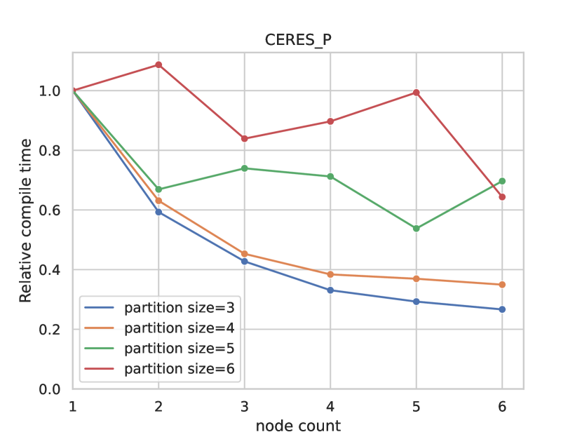
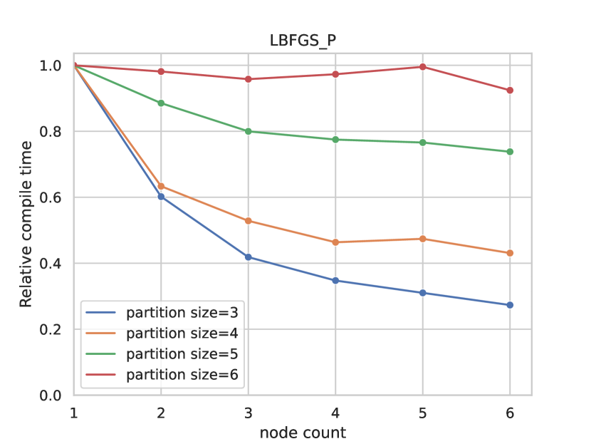
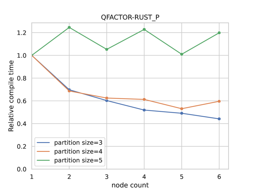
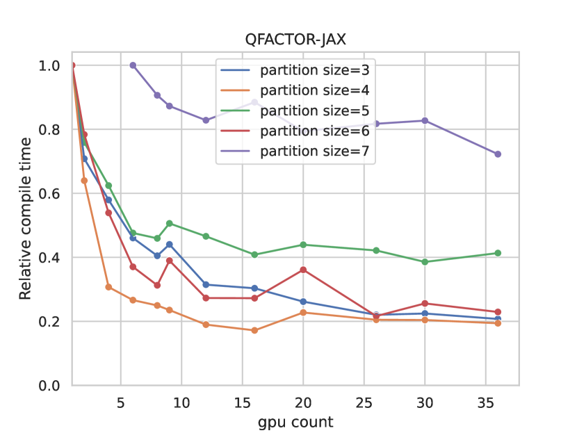
Figure 6: Strong scaling of compilation of large circuits. Relative compilation run time of different instantiators, across various partition sizes with varying resources, showing strong parallelization. Performance is normalized to either 1 CPU node, or to 1 GPU device respectively, unless it timed out, then it’s for 2 resources.

V-C Circuit Optimization Efficacy

To assess efficacy we measure the number of gates deleted by this pass for increasing partition size and report their average. For each flow configuration, we use the same input set of circuits. Due to the 11 hours compilation time limit and the differences in execution time between optimizers, we note that increasing the partition size decreases the number of successful jobs due to timeouts. We also don’t initiate a circuit compilation with a bigger partition size, if a lower one timed out. Furthermore, for a given partition size we note that a different set of circuits may be successfully optimized by a flow configuration.

Figure 7 presents the average reduction in U3 and CNOT gates when increasing the number of qubits within a partition. As shown, the ability to process nine qubit partitions leads to $4\times$ and $2\times$ increases in the number of U3 and CNOT gates deleted, respectively. The GPU implementation of $QFactor\$is the only instantiator that didn’t cause a time out for partition sizes of 8 and 9. For three- to five-qubit partitions the quality of output is comparable. We also note that $QFactor\$and LBFGS particularly struggle on the Hubbard model circuits, while CERES is able to find a more efficient implementation. For $QFactor\$hyperparameter tuning may be used to improve efficacy.

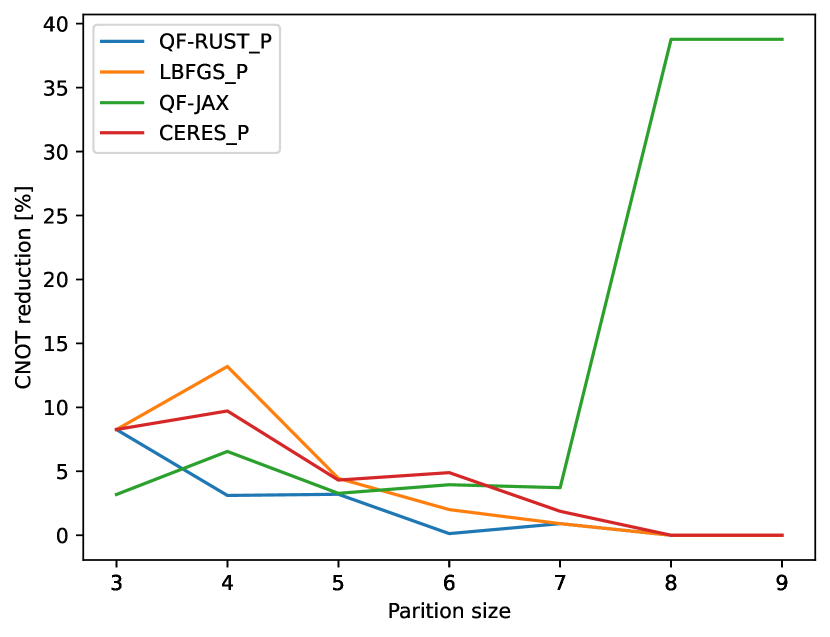
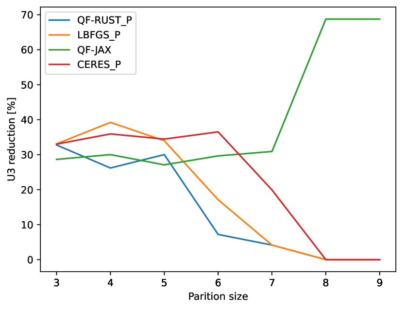
Figure 7: Average percentage of CNOT and U3 reduction in the gate deletion flow.

For a more detailed understanding of the dynamics, we split the input circuits by size into three buckets: small - up to 9 qubits, medium - 10-36 qubits, and large - 36 and above qubits. The data is presented in Figure 8. For the small circuits, due to its better scalability $QFactor\$reduces gate count by an “average” of 40%, and CERES by an ”average” of 25%.

The dynamics for 3- to 6-qubit partitions for both optimizers are explained by the composition of the data set: for small circuits a partition may cover a very large fraction of the original circuit, thus capturing complex physical interactions present in the domain science problem formulation. On the other hand, when partitioning a larger circuit, the partitions are likely to be themselves ”simple” circuits. Intuitively, the bigger the fraction of a circuit a partition covers, the bigger the chance it may capture complex interactions between qubits as determined by the domain science behind the particular algorithm. This also explains some of the differences in the quality of optimization between the medium and large circuits buckets. The impact of circuit size and the time limit can also be observed: large circuits have more partitions and their jobs time out more when increasing partition size, as they form more complex partitions.

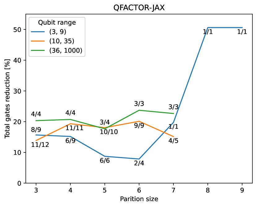
Figure 8: Average percentage of total gate reduction in the gate deletion flow divided into buckets according to the amount of qubits in the circuit, CERES_P and QF-JAX are shown. For each data partition size and bucket, also show how many circuits were successful.

Circuit	U3	CNOT
adder9	64	98
add17	348	232
adder63	2885	1405
mult8	210	188
mult16	1264	1128
grover5	80	48
hhl8	3288	2421
shor26	20896	21072
hub4	155	180
hub18	1992	3541
heis7	490	360
heis8	570	420
heis64	5050	3780
tfim8	428	280
tfim16	916	600
tfim400	88235	87670
qae11	176	110
qae13	247	156
qae33	1617	1056
qae81	7341	4840
qaoa5	27	42
qaoa10	40	85
qaoa12	90	198
vqe5	132	91
vqe12	4157	7640
vqe14	10792	20392
qpe8	519	372
qpe10	1681	1260
qpe12	3582	2550

Table III: Benchmarks and their gate counts, upper bound of $\approx 200,000$. The name suffix represents the number of qubits in the circuit, up to 400 qubits.

VI Discussion

The results indicate that $QFactor\$greatly accelerates the performance of instantiation and it enables us to handle larger volume circuits. Both general-purpose optimizers and $QFactor\$scale exponentially with parameters. Instantiation with GPO algorithms use parameterized gates: CERES and LBFGS formulations treat an U3 gate as three parameters. $QFactor\$treats it as a single parameter benefiting from memory reduction and is most likely simpler to optimize objective functions. Moreover, $QFactor\$can be generalized to treat multi-qubit ($n>2$) unitaries as a single parameter for further scalability improvements, while GPOs still have to represent these with $O(2^{n})$ parameters. This generalization is likely to improve the performance of $QFactor\$even further.

Figure 7 shows the evolution with partition size of the quality of solutions generated by the gate deletion workflow. These clearly indicate that when incorporated into circuit optimization compiler passes, $QFactor\$improves the quality of the generated circuit when compared against general-purpose optimizers.

The observed dynamics of compilation time and output circuit quality with $QFactor\$enable us to draw very useful conclusions with respect to architecting instantiation or synthesis based workflows for large circuits.

The improvement in gate count reduction seems to grow with the partition size, while numerical optimization algorithms usually scale exponentially. This opens the door for configuring compiler workflows based on tradeoffs between output quality and compilation speed. Furthermore, if compilation speed is important, generating three qubit partitions seems to provide a good default.

Another very interesting question is finding the partition size that maximizes the quality of large circuit optimizations: Is it a function of circuit size and structure? The answer may guide future research attempts to scale direct unitary instantiation (numerical optimization) and synthesis algorithms (search over circuit structures and numerical optimization) with qubits.

A partial answer provided by this study is that, for circuits with many qubits, the efficacy of circuit optimizations using instantiation saturates with partitions of 5-7 qubits. These partitions seem to be the sweet spot for numerical optimization with $QFactor$or CERES. While for this submission we show results for gate deletion in large circuits using partitions up to 9 qubits, we have started experiments for partitions up to 12 qubits to understand better the $QFactor\$dynamics.

This needs more investigation, and the reasoning is more subtle. The real metric is probably the ratio of circuit gates to partition gates rather than number of qubits, augmented by structure imposed by domain science. Algorithms are written in terms of qubit interactions. Whenever a partition captures the totality of interactions between groups of qubits, direct optimization will see great benefits. Otherwise, we expect to see the same saturation in the quality of the circuit optimization.

Based on these considerations, and to conserve the limited Perlmutter supercomputing allocation, we have stopped our instantiation experimentation at partitions with only 12 qubits. The experimental data clearly indicates that $QFactor\$is able to process even larger circuits. Note that we have used +20K hybrid GPU node hours and +13K CPU node hours. This amounts to $20K\times(4GPUs+64\ cores)$ and $13K\times 128\ cores$ physical resources. We thank the NERSC directorate for allowing us to run on their discretionary allocation.

Due to the tensor network formulation, our algorithm formulation benefits greatly from GPU acceleration. We have not tuned at all the GPU resource allocation strategy for compilations of four- to 12 qubit circuits. As both the number of qubits and the number of gates determines performance, additional improvements are likely to be had by a more judicious resource allocation on GPUs.

Numerical optimization behavior is notoriously fickle and requires customization for the problem at hand. For this study we performed only minimal tuning of the $QFactor\$parameters. As each instantiated circuit has a different structure, therefore leading to a different optimization surface, we believe we can improve both performance and quality of optimization with parameter tuning.

The results were demonstrated on a U3+CNOT gate set. $QFactor\$is easily portable to other gate sets, all that it requires is providing derivatives. An interesting question remains if adopting a different gate set changes the conclusions of this paper.

VII Conclusion

We introduce $QFactor$, a domain specific optimizer designed for quantum circuit instantiation problems. When compared against general purpose optimizers $QFactor\$scales better and is able to process much larger circuits. When replacing general purpose optimizers with $QFactor\$into a compilation workflow, this capability translates into better optimized circuits. Due to its formulation $QFactor\$is able to execute on GPUs and benefit from their hardware acceleration. Furthermore, the $QFactor\$enabled compiler running on GPUs seems to scale out linearly in distributed memory environments; this does not happen for CPU based compiler workflows, regardless of the numerical optimizer. This bodes well for the more general adoption of synthesis based quantum circuit optimizations: while their efficacy in optimizing circuits is recognized, adoption is hampered by runtime overhead. By significantly improving circuit quality and scaling in distributed memory GPU based environments $QFactor\$provides a first good step into alleviating execution overhead concerns.

References

- [1] J. R. McClean, J. Romero, R. Babbush, and A. Aspuru-Guzik, “The theory of variational hybrid quantum-classical algorithms,” New Journal of Physics, vol. 18, no. 2, p. 023023, 2016.
- [2] E. Farhi, J. Goldstone, and S. Gutmann, “A quantum approximate optimization algorithm,” arXiv preprint arXiv:1411.4028, 2014.
- [3] Q. Developers, “Qiskit: An Open-source Framework for Quantum Computing,” Jan. 2019.
- [4] C. Developers, “Cirq,” Aug. 2021. See full list of authors on Github: https://github .com/quantumlib/Cirq/graphs/contributors.
- [5] S. Sivarajah, S. Dilkes, A. Cowtan, W. Simmons, A. Edgington, and R. Duncan, “t— ket¿: a retargetable compiler for nisq devices,” Quantum Science and Technology, vol. 6, no. 1, p. 014003, 2020.
- [6] E. Younis, C. C. Iancu, W. Lavrijsen, M. Davis, E. Smith, et al., “Berkeley quantum synthesis toolkit (bqskit) v1,” 2021.
- [7] E. Younis, K. Sen, K. Yelick, and C. Iancu, “Qfast: Conflating search and numerical optimization for scalable quantum circuit synthesis,” in 2021 IEEE International Conference on Quantum Computing and Engineering (QCE), pp. 232–243, IEEE, 2021.
- [8] M. G. Davis, E. Smith, A. Tudor, K. Sen, I. Siddiqi, and C. Iancu, “Towards optimal topology aware quantum circuit synthesis,” in 2020 IEEE International Conference on Quantum Computing and Engineering (QCE), pp. 223–234, IEEE, 2020.
- [9] E. Younis and C. Iancu, “Quantum circuit optimization and transpilation via parameterized circuit instantiation,” in 2022 IEEE International Conference on Quantum Computing and Engineering (QCE), (Los Alamitos, CA, USA), pp. 465–475, IEEE Computer Society, sep 2022.
- [10] L. Cincio, K. Rudinger, M. Sarovar, and P. J. Coles, “Machine learning of noise-resilient quantum circuits,” PRX Quantum, vol. 2, no. 1, p. 010324, 2021.
- [11] P. Rakyta and Z. Zimborás, “Approaching the theoretical limit in quantum gate decomposition,” 2021.
- [12] P. Rakyta and Z. Zimborás, “Efficient quantum gate decomposition via adaptive circuit compression,” 2022.
- [13] N. A. Nemkov, E. O. Kiktenko, I. A. Luchnikov, and A. K. Fedorov, “Efficient variational synthesis of quantum circuits with coherent multi-start optimization,” arXiv preprint arXiv:2205.01121, 2022.
- [14] C. Guo, Y. Zhao, and H.-L. Huang, “Verifying random quantum circuits with arbitrary geometry using tensor network states algorithm,” Physical Review Letters, vol. 126, no. 7, p. 070502, 2021.
- [15] T. Nguyen, D. Lyakh, E. Dumitrescu, D. Clark, J. Larkin, and A. McCaskey, “Tensor network quantum virtual machine for simulating quantum circuits at exascale,” ACM Transactions on Quantum Computing, vol. 4, no. 1, pp. 1–21, 2022.
- [16] F. Pan and P. Zhang, “Simulation of quantum circuits using the big-batch tensor network method,” Physical Review Letters, vol. 128, no. 3, p. 030501, 2022.
- [17] J. Chen, E. Stoudenmire, and S. R. White, “The quantum fourier transform has small entanglement,” arXiv preprint arXiv:2210.08468, 2022.
- [18] T. Vincent, L. J. O’Riordan, M. Andrenkov, J. Brown, N. Killoran, H. Qi, and I. Dhand, “Jet: Fast quantum circuit simulations with parallel task-based tensor-network contraction,” Quantum, vol. 6, p. 709, 2022.
- [19] C. Mc Keever and M. Lubasch, “Classically optimized hamiltonian simulation,” Phys. Rev. Res., vol. 5, p. 023146, Jun 2023.
- [20] J. Bradbury, R. Frostig, P. Hawkins, M. J. Johnson, C. Leary, D. Maclaurin, G. Necula, A. Paszke, J. VanderPlas, S. Wanderman-Milne, and Q. Zhang, “JAX: composable transformations of Python+NumPy programs,” 2018.
- [21] S. Agarwal, K. Mierle, and T. C. S. Team, “Ceres Solver,” 3 2022.
- [22] S. G. Johnson, “The nlopt nonlinear-optimization package.”
- [23] D. C. Liu and J. Nocedal, “On the limited memory bfgs method for large scale optimization,” Mathematical programming, vol. 45, no. 1-3, pp. 503–528, 1989.
- [24] J. Nocedal, “Updating quasi-newton matrices with limited storage,” Mathematics of computation, vol. 35, no. 151, pp. 773–782, 1980.
- [25] M. C. Caro, H.-Y. Huang, M. Cerezo, K. Sharma, A. Sornborger, L. Cincio, and P. J. Coles, “Generalization in quantum machine learning from few training data,” Nature communications, vol. 13, no. 1, p. 4919, 2022.
- [26] T. Eckstein, R. Mansuroglu, P. Czarnik, J.-X. Zhu, M. J. Hartmann, L. Cincio, A. T. Sornborger, and Z. Holmes, “Large-scale simulations of floquet physics on near-term quantum computers,” arXiv preprint arXiv:2303.02209, 2023.
- [27] M. C. Caro, H.-Y. Huang, N. Ezzell, J. Gibbs, A. T. Sornborger, L. Cincio, P. J. Coles, and Z. Holmes, “Out-of-distribution generalization for learning quantum dynamics,” arXiv preprint arXiv:2204.10268, 2022.
- [28] M. Bilkis, M. Cerezo, G. Verdon, P. J. Coles, and L. Cincio, “A semi-agnostic ansatz with variable structure for quantum machine learning,” arXiv preprint arXiv:2103.06712, 2021.
- [29] R. R. Tucci, “An introduction to cartan’s kak decomposition for qc programmers,” arXiv preprint quant-ph/0507171, 2005.
- [30] L. Madden and A. Simonetto, “Best approximate quantum compiling problems,” ACM Transactions on Quantum Computing, vol. 3, mar 2022.
- [31] A. Ranganathan, “The levenberg-marquardt algorithm,” Tutoral on LM algorithm, vol. 11, no. 1, pp. 101–110, 2004.
- [32] W. Lavrijsen, A. Tudor, J. Muller, C. Iancu, and W. de Jong, “Classical optimizers for noisy intermediate-scale quantum devices,” in 2020 IEEE International Conference on Quantum Computing and Engineering (QCE), (Los Alamitos, CA, USA), pp. 267–277, IEEE Computer Society, oct 2020.
- [33] C. T. Kelley, Implicit Filtering. Society for Industrial and Applied Mathematics, 2011.
- [34] S. Le Digabel, “Nomad: Nonlinear optimization with the mads algorithm,” ACM Trans. Math. Softw., vol. 37, p. 44, 01 2011.
- [35] W. Huyer and A. Neumaier, “Snobfit - stable noisy optimization by branch and fit,” ACM Trans. Math. Softw., vol. 35, 07 2008.
- [36] C. Cartis, J. Fiala, B. Marteau, and L. Roberts, “Improving the flexibility and robustness of model-based derivative-free optimization solvers,” 2018.
- [37] C. Cartis, L. Roberts, and O. Sheridan-Methven, “Escaping local minima with derivative-free methods: a numerical investigation,” 2019.
- [38] X.-C. Wu, M. G. Davis, F. T. Chong, and C. Iancu, “Reoptimization of quantum circuits via hierarchical synthesis,” in 2021 International Conference on Rebooting Computing (ICRC), pp. 35–46, 2021.
- [39] R. Orús, “A practical introduction to tensor networks: Matrix product states and projected entangled pair states,” Annals of physics, vol. 349, pp. 117–158, 2014.
- [40] K. Wright, K. M. Beck, S. Debnath, J. M. Amini, Y. Nam, N. Grzesiak, J.-S. Chen, N. C. Pisenti, M. Chmielewski, C. Collins, K. M. Hudek, J. Mizrahi, J. D. Wong-Campos, S. Allen, J. Apisdorf, P. Solomon, M. Williams, A. M. Ducore, A. Blinov, S. M. Kreikemeier, V. Chaplin, M. Keesan, C. Monroe, and J. Kim, “Benchmarking an 11-qubit quantum computer,” Nature Communications, vol. 10, p. 5464, Nov. 2019.
- [41] K. Mølmer and A. Sørensen, “Multiparticle entanglement of hot trapped ions,” Phys. Rev. Lett., vol. 82, pp. 1835–1838, Mar 1999.
- [42] NVIDIA, “Multi-process service (mps).” https://docs.nvidia.com/deploy/mps/index.html, 2021.
- [43] H. Khetawat, M. Hassan, A. Neri, A. Rodrigues, and T. Wong, “QArithmetic.”
- [44] P. W. Shor, “Polynomial-time algorithms for prime factorization and discrete logarithms on a quantum computer,” SIAM review, vol. 41, no. 2, pp. 303–332, 1999.
- [45] L. K. Grover, “A fast quantum mechanical algorithm for database search,” in Proceedings of the twenty-eighth annual ACM symposium on Theory of computing, pp. 212–219, 1996.
- [46] A. Kandala, A. Mezzacapo, K. Temme, M. Takita, M. Brink, J. M. Chow, and J. M. Gambetta, “Hardware-efficient variational quantum eigensolver for small molecules and quantum magnets,” Nature, vol. 549, no. 7671, pp. 242–246, 2017.
- [47] S. B. Bravyi and A. Y. Kitaev, “Fermionic quantum computation,” Annals of Physics, vol. 298, no. 1, pp. 210–226, 2002.
- [48] J. Hubbard, “Electron correlations in narrow energy bands,” Proceedings of the Royal Society of London. Series A. Mathematical and Physical Sciences, vol. 276, no. 1365, pp. 238–257, 1963.
- [49] D. Shin, H. Hübener, U. De Giovannini, H. Jin, A. Rubio, and N. Park, “Phonon-driven spin-floquet magneto-valleytronics in mos_2,” Nature Communications, vol. 9, no. 1, p. 638, 2018.
- [50] L. Bassman, C. Powers, and W. A. de Jong, “ArQTiC: A full-stack software package for simulating materials on quantum computers,” 2021.
- [51] “Qce23 qfactor benchmarks.” https://github.com/BQSKit/qce23_qfactor_benchmarks, 2023.
- [52] E. Smith, M. G. Davis, J. Larson, E. Younis, L. B. Oftelie, W. Lavrijsen, and C. Iancu, “Leap: Scaling numerical optimization based synthesis using an incremental approach,” ACM Transactions on Quantum Computing, vol. 4, feb 2023.
- [53] “Perlmutter architecture.” https://docs.nersc.gov/systems/perlmutter/architecture/, 2023.
- [54] T. Patel, E. Younis, C. Iancu, W. de Jong, and D. Tiwari, “Quest: systematically approximating quantum circuits for higher output fidelity,” in Proceedings of the 27th ACM International Conference on Architectural Support for Programming Languages and Operating Systems, pp. 514–528, 2022.