Dark matter search with a strongly-coupled hybrid spin system

Abstract

Observational evidence suggests the existence of dark matter (DM), which comprises approximately $84.4\%$ of matter in the universe. Recent advances in tabletop quantum sensor technology have enabled searches for nongravitational interactions of DM. Our experiment named ChangE utilizes Coupled Hot Atom eNsembles to search for liGht dark mattEr and new physics. We identify a strongly-coupled hybrid spin-resonance (HSR) regime that enhances the bandwidth of ²¹Ne nuclear spin by three orders of magnitude while maintaining high sensitivity. In combination with a self-compensating mode (SC) for low frequencies, we present a comprehensive broadband search for axion-like dark matter with Compton frequencies in the range of $[0.01,1000]$ Hz. We set new constraints on the DM interactions with neutrons and protons, accounting for the stochastic effect. For the axion-neutron coupling, our results reach a low value of $|g_{ann}|\leq 3\times 10^{-10}$ in the frequency range $[0.02,4]$ Hz surpassing astrophysical limits and provide the strongest laboratory constraints in the $[10,100]$ Hz range. For the axion-proton coupling, we offer the best terrestrial constraints for the frequency below 100 Hz.

Introduction. There is evidence of dark matter (DM) from numerous astrophysical and cosmological observations. However, its nature is yet to be understood, which is one of the most important challenges in modern physics. Ultralight pseudoscalar particles, such as axions or axionlike particles (ALPs) Essig:2013lka ; ParticleDataGroup:2020ssz , are well-motivated dark matter candidates, which can be produced via the “misalignment mechanism” to obtain the correct relic abundance Duffy:2009ig ; Marsh:2015xka . The axion is particularly well motivated as it also solves the so-called strong-CP problem by introducing the Peccei-Quinn global symmetry Peccei:1977hh ; Peccei:1977ur ; Weinberg:1977ma ; Wilczek:1977pj ; Vafa:1984xg . It (weakly) couples to other particles Golub:1994cg due the spontaneous braking of this symmetry at a high energy. In this article, we refer to both axions and ALPs as “axions”, so that the coupling to photons, gluons and fermions can span a wide range of parameter space which has been explored in various astrophysical and laboratory experiments Raffelt:1990yz ; Graham:2015ouw ; Safronova:2017xyt .

Regarding the coupling to nucleons, the axion gradient field can be measured as an anomalous magnetic field coupling to the nuclei. In the non-relativistic limit, the gradient interaction can be described by the Hamiltonian

$$\mathcal{H}=g_{aNN}\bm{\nabla}a\cdot\bm{\sigma}_{N},$$ (1)

where $\sigma_{N}$ is the spin of the nucleus which includes fraction of spins of the neutron and proton, and $g_{aNN}$ is the effective axion coupling to the nucleus. Therefore, the anomalous magnetic field due to the axion DM is $\bm{b}_{a}\equiv g_{aNN}\bm{\nabla}a/\gamma_{n}$, where $\gamma_{n}$ is the gyromagnetic ratio of the nuclear spin.

Recent experiments are using various nuclei, including the liquid state experiments using proton and ¹³C wu2019search and gas state sensors based on alkali-noble pairs using ³He bloch2020axion ; bloch2022nasduck ; Bloch:2019lcy ; Lee:2022vvb and ¹²⁹Xe Jiang:2021dby . These terrestrial experiments explore the nuclear precession frequency range from  $\mu$Hz to hundreds of kHz, corresponding to the axion mass range from 10^-22 to 10^-10 eV. In the frequency range from approximately 0.1 Hz to 10 Hz, the ³He comagnetometer sets limits on the axion-neutron coupling to be lower than 10${}^{-9}\,\rm{GeV}^{-1}$ Lee:2022vvb , which is tighter than the astrophysical limits set by the cooling process of supernova Carenza:2019pxu and neutron stars Buschmann:2021juv .

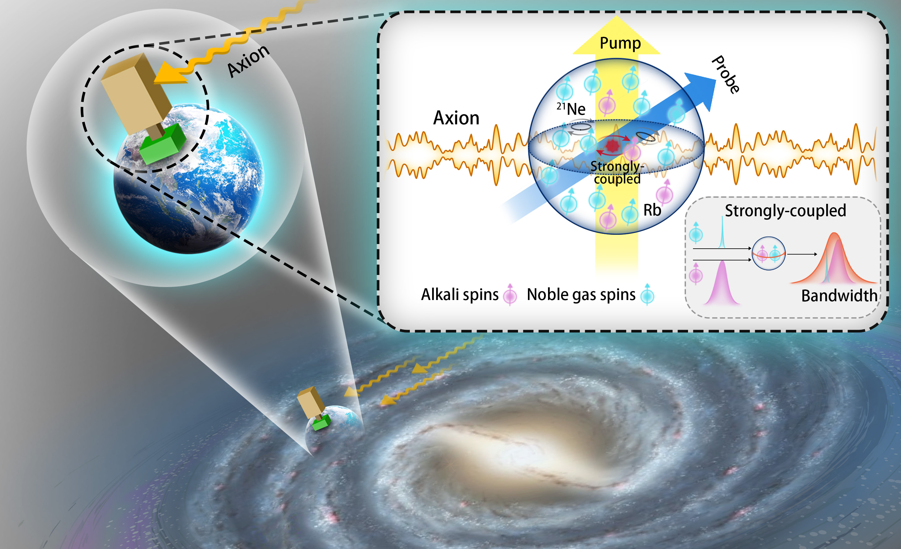
Figure 1: The dark matter detection principle is as follows: (1) Pump light polarizes the alkali electron spins, while spin-exchange collisions with alkali spins polarize the noble-gas nuclear spins. (2) The axion dark matter produced a pseudomagnetic field acting on nuclear spins. The nuclear spins precess due to excitation from the axion field, and this precession is transferred to alkali spins via spin-exchange collisions. (3) The resulting precession of the alkali spins is read out using optical rotation of the probe light. Normally, the measurement bandwidth of noble-gas nuclear spins is narrow due to their small relaxation rate $\Gamma_{n}$, which is several orders of magnitude smaller than that of alkali spins. However, in the HSR regime, the noble-gas spins become strongly coupled with alkali spins. As a result, the interactions with alkali-metal spins significantly broaden the bandwidth of the noble-gas spins.

Typically, to expand the search range for DM with gas-state quantum sensors, a bias magnetic field is applied. In bloch2022nasduck , a spin-exchange-relaxation-free (SERF) magnetometer used with a leading field that is sufficiently high to break the SERF regime, leading to increased spin-exchange relaxation. In Jiang:2021dby , a spin-based amplifier is applied, where the resonance frequency is scanned by adjusting the external magnetic field to match the Larmor frequency with the axion Compton frequency. Resonant searches benefit from high Q factors at the resonant frequency but suffer from narrow bandwidth, typically at the level of 0.01 Hz. Thus, to search for an axion with unknown mass, one needs to scan the frequency with steps corresponding to the narrow bandwidth to cover the target frequency range, rendering resonant searches to be time-consuming.

In this work, we demonstrate a strongly-coupled Hybrid Spin-Resonance (HSR) regime of the alkali-noble sensor with about three orders of magnitude improvement in bandwidth. This bandwidth boost is achieved by hybridizing the noble-gas and alkali spin resonances. Thus the noble-gas spins “mimic” the dynamic performance of alkali spins. Compared to the operation of K-³He spins in the fast-damping regime lee2019new , HSR employs the alkali-noble-gas spin system with stronger Fermi-contact-interaction (FCI). In our experiment with a Rb-²¹Ne mixture, the Fermi-contact field is two orders of magnitude higher than that in the K-³He work lee2019new , which we use to further improve the dynamic performance of the system without compromising its sensitivity. We report a magnetic field sensitivity of 0.78 fT/$\sqrt{\rm{Hz}}$ in the frequency range from 28 to 32 Hz in HSR regime, which represents a significant improvement over the previous work addressing this frequency range Jiang:2021dby . We also tune the comagnetometer to work in the self-compensating regime to measure the exotic field in the frequency range from 0.01 to 10 Hz, whose sensitivity to the pseudomagnetic field coupling to noble-gas spin is about 1.5 fT/$\sqrt{\rm{Hz}}$ around 0.1 to 1 Hz. We operate the alkali-noble sensor in the HSR and SC regimes to measure DM in a broadband from 0.01 to 1000 Hz.

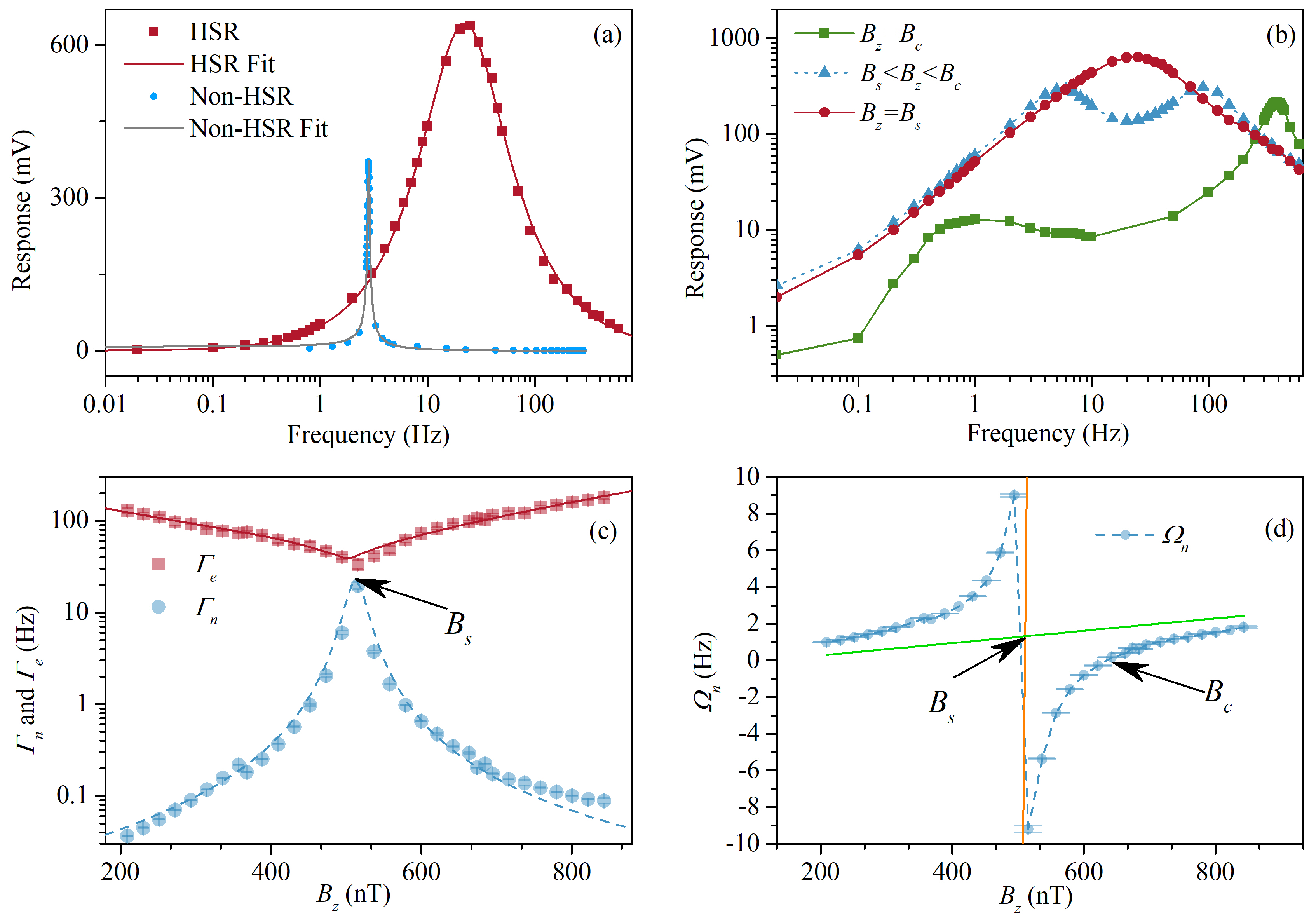
Figure 2: Proof-of-principle demonstration of a hybrid strongly-coupled spin resonance. (a) Comparison of the HSR and non-HSR regimes. The bandwidth of HSR is more than three orders of magnitude higher than for non-HSR. (b) Response to an oscillating magnetic field applied along $\hat{x}$ as a function of the oscillation frequency. Outside the HSR regime, there are two peaks in the response that merge into one broad peak when the bias field $B_{z}$ is tuned to achieve the HSR. $B_{s}$ is the strong-coupling point, $B_{c}$ is the self-compensation point. (c) The change of the relaxation rates $\Gamma_{\rm{e(n)}}$ of the transverse spin components of alkali-metal spins and noble-gas spins. $\Gamma_{\rm{e}}$ decreases as the bias field approaches the HSR value $B_{s}$, while $\Gamma_{\rm{n}}$ increases significantly, by more than three orders of magnitude. The relaxation rates are determined from fitting the response to a step in the $B_{x}$ field to a Bloch-equation model. (d) The precession frequency $\Omega_{\rm{n}}$ of noble-gas nuclear spins as a function of the bias field. The yellow asymptotic line is the precession rate of alkali spins only, while the green asymptotic line is the precession of noble-gas spins. Note the linear vertical scale in (a) and (d) and logarithmic scales in (b) and (c).

Basic Principle of Magnetometer. In this work, we use a ²¹Ne-Rb-K vapor-cell magnetometer, in which the minority potassium atoms are used for “hybrid optical pumping” babcock2003hybrid ; romalis2010hybrid and the mixed-spin ensemble of rubidium and neon are operated in a regime where the two spin species are strongly coupled giving rise to a hybrid magnetic resonance . The alkali-metal atoms (K and Rb) and the ²¹Ne isotope (0.27% natural abundance enriched to 70%) are contained in a spherical 11.4 mm internal diameter glass cell. The alkali-metal atoms are spin-polarized with circularly-polarized light tuned to the potassium D1 line. The spin angular momentum is transferred from the “minority” K atoms to the Rb atoms and the ²¹Ne nuclear spins via spin-exchange (SE) collisions. The hybrid-pumping is used to improve the hyperpolarization efficiency for ²¹Ne nuclear spins and reduce the polarization gradient of alkali-metal spins, which is achieved by optically pumping the optically-thin potassium vapor to avoid strong resonant absorption of the pump light wei2022constraints ; Wei:2022ggs . The precession of polarized ²¹Ne nuclear spins is monitored with optically-thick Rb spins, read out by detecting optical rotation of linearly-polarized probe light detuned to longer wavelengths from the D1 line of Rb.

The spin interactions between hyperpolarized ²¹Ne atoms and spin-polarized alkali-metal atoms are dominated by Fermi-contact interactions, which can be characterized as effective fields ${\bf{\hat{B}^{e/n}}}=\lambda M^{\rm{e/n}}_{0}{\bf{P^{e/n}}}$ due to the magnetization of the other spin species, where $\lambda$ is the Fermi-contact enhancement factor, $M^{\rm{e/n}}_{0}$ is magnetization of alkali-metal (noble-gas) atoms for fully polarization, ${\bf{P^{e/n}}}$ is the collective spin polarization of alkali-metal (noble-gas) spin ensembles. Therefore, the total fields experienced by alkali-metal spins and noble-gas spins are ${\bf{B^{e}}}={\bf{\hat{B}^{n}}}+{\bf{B}}$ and ${\bf{B^{n}}}={\bf{\hat{B}^{e}}}+{\bf{B}}$, respectively, where ${\bf{B}}$ is the applied magnetic field. Typically, owing to the difference in the gyromagnetic ratio of alkali-metal spins and noble-gas nuclear spins, the Larmor frequency of alkali-metal spins at a given field is orders of magnitude higher than that of noble-gas spins.

We find the Larmor frequency of alkali-metal spins can be slowed down by adjusting ${\bf{B}}$ to cancel out ${\bf{\hat{B}^{n}}}$. Meanwhile, the Larmor frequency of noble-gas spins can be simultaneously accelerated, because the noble-gas spins do not feel their own ${\bf{\hat{B}^{n}}}$. In this way, the frequencies of alkali-metal spins and noble-gas spins can be tuned close to each other. Due to the FCI interaction between them, they become strongly coupled in this state and precess together. This is the essence of HSR, where the damping rate of alkali-metal spins is slowed down by noble-gas spins, while that of the noble-gas spins is accelerated by the alkali-metal spins. Therefore, the bandwidth of noble-gas nuclear spins can be increased by orders of magnitude.

We experimentally demonstrate the hybrid strongly-coupled spin resonance as shown in Fig. 2. The response of the alkali-noble-gas spins to an oscillating magnetic field is shown in Fig. 2(a) outside of (blue) and within (red) the strong-coupling regime. In the former case, the bandwidth $\Delta v$ is $\approx$0.01 Hz, which is also the typical bandwidth of spin amplifiers Jiang:2021dby . By operating the noble-gas and alkali-metal spin ensembles in the strong-coupling regime, the response to magnetic field is broadened by three orders of magnitude.

This broadening is achieved by setting the bias field $B_{z}$ to the strong-coupling value $B_{s}\approx-\hat{B}^{n}_{z}$. As shown in Fig. 2(b), when instead we set the bias field $B_{z}$ to other value, such as the self-compensating point $B_{c}=-\hat{B}^{e}_{z}-\hat{B}^{n}_{z}$, there are two separate peaks in the frequency response. The low-frequency one is from noble-gas nuclear spins, while the high-frequency one is from alkali-metal spins. When we set the bias field $B_{z}$ in between the self-compensation point $B_{c}$ and the strong-coupling point $B_{s}$, the response peaks of noble-gas nuclear spins and alkali-metal spins move closer. Finally, When the bias field is set to the strong-coupling point, the two peaks merge.

To present the changes in bandwidth of alkali-metal spins and noble-gas spins, we measure the relaxation rate (damping rate) of the transverse spin component of two spin species respectively. As shown in Fig. 2(c), the damping rate $\Gamma_{\rm{e}}$ of alkali electron spins decreases as the bias field $B_{z}$ approaches the strong-coupling point, while the damping rate $\Gamma_{\rm{n}}$ of noble-gas nuclear spins increases for three orders of magnitude. This result intuitively presents that the alkali-metal electron spins are slowed down by strong coupling with noble-gas nuclear spins, while the noble-gas nuclear spins are speed up. Therefore, the hybrid response peak is no longer contributed by two spin species separately. Rather, the peak is due to the coupled-hybrid spin ensemble. The bandwidth of the HSR is a hybrid combination of $\Gamma_{\rm{e}}$, $\Gamma_{\rm{n}}$, ${\hat{B}^{e}_{z}}$, and ${\hat{B}^{n}_{z}}$, and also depends on the bias field $B_{z}$ (details in Supplementary). As shown in Fig. 2(d), the precession of the spins changes direction at the strong-coupling point $B_{s}$. In this region, the overall magnetic-field response is dominated by the alkali spins. Away from the strong-coupling point, the precession frequency $\Omega_{\rm{n}}$ gradually approaches the asymptotic frequency dependence for uncoupled noble-gas spins, $\Omega_{\rm{n}}=\gamma_{n}B_{z}$.

We now discuss the magnetic and dark-matter sensitivity of the hybrid strongly-coupled resonance regime, see Fig. 3. The sensitivity is calibrated by applying oscillating magnetic fields generated with a magnetic coil. The sensitivity reaches 0.78 fT/Hz^1/2 from 28 to 32 Hz, which is among the most sensitive magnetometers using alkali-metal spins to read out the noble-gas nuclear spins. The sensitivity is more than one order of magnitude better than the state-of-art spin amplification jiang2021floquet . The noise peaks around 6 Hz and from 17 to 23 Hz are due to the vibrations, which is confirmed using a commercial seismometer. The peak at 50 Hz is due to the power line. The magnetic noise of the inner Mn-Zn ferrite shield in the relevant frequency range is estimated to be kornack2007low 2.5 $f^{-1/2}$ fT ($f$ is the frequency in Hz), using the measured relative permeability and geometrical parameters of the shield. Details about vibration and magnetic noise can be found in the supplementary in Ref. wei2022constraints . This means that the estimated magnetic noise from the shield is close to the total noise level. The background noise of the probe with pump light blocked is about 0.2 fT/Hz^1/2 from 28 to 32 Hz, which is significantly smaller than the total noise. The spin-projection noise of alkali spins is calculated to be about 0.09 fT/Hz^1/2 kornack2005nuclear . In HSR, the relationship between the response to ultra-light dark matter field $b^{n}_{x}$ coupling with noble-gas nuclear spins $S^{e}_{x}=K_{b^{n}_{x}}b^{n}_{x}$ and the response to magnetic field $S^{e}_{x}=K_{B_{y}}B_{y}$ is $K_{B_{y}}=K_{b^{n}_{x}}\omega/\hat{\omega}^{n}_{z}$, where $\hat{\omega}^{n}_{z}=\gamma_{n}\hat{B}^{n}_{z}$ , $\omega$ is the frequency of the signal $b^{n}_{x}$. Therefore, we can use the magnetic field to calibrate the response to $b^{n}_{x}$.

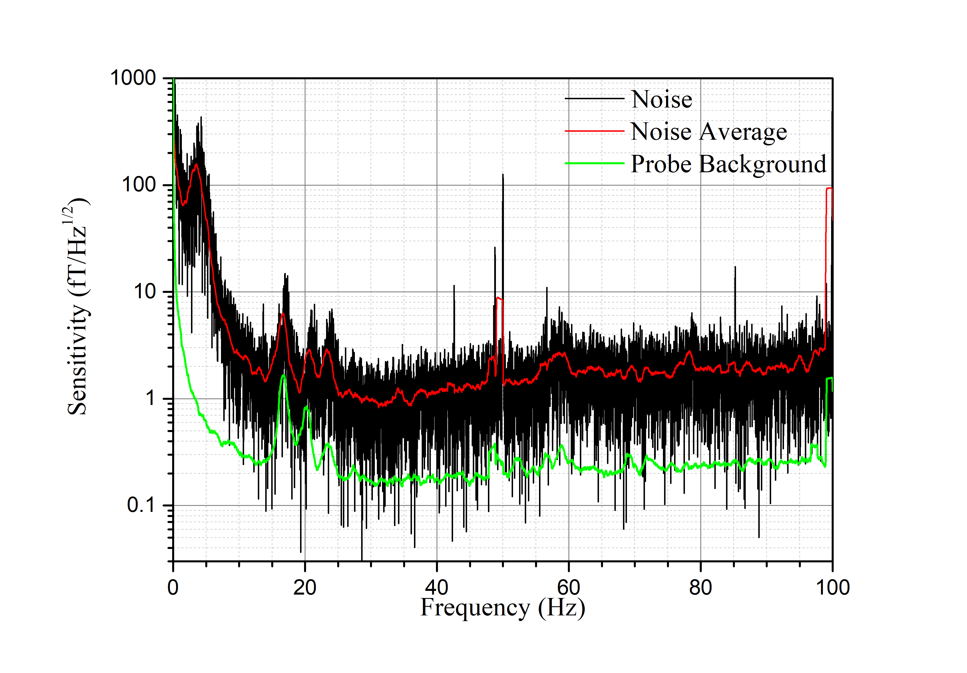
Figure 3: The sensitivity at the strongly coupled hybrid spin resonance to a $\hat{y}$-directed magnetic field is 0.78 fT/Hz^1/2 from 28 to 32 Hz, placing the system among the most sensitive sensors using alkali-metal spins to measure the precession of noble-gas nuclear spins. The noise peaks around 6 Hz, and from 17 to 23 Hz are due to the vibrations, which is verified with a seismometer. The noise peak at 50 Hz is the power-line noise. The background noise of probe with pump light blocked is much smaller than total noise level.

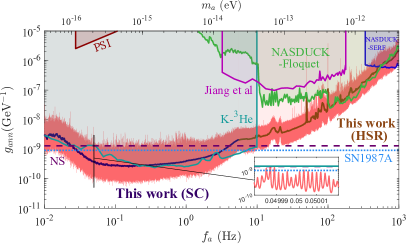
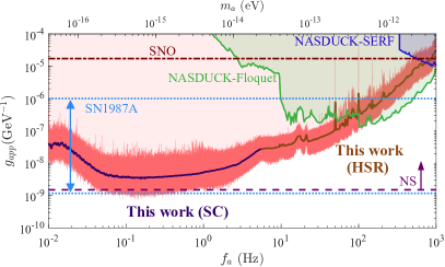
Figure 4: The $95\%$ C.L. upper limits (red lines) for axion-neutron coupling $g_{ann}$ and axion-proton coupling $g_{app}$ from measurements in both the self-compensating (SC) and hybrid spin-resonance (HSR) regimes. The full data of the limits cannot be shown in the figure, but are tabulated in axiondata . To guide the readers’ eye, for each $f_{a}$, the couplings $g_{ann}$ and $g_{app}$ are averaged in a bin from $0.99f_{a}$ to $1.01f_{a}$. We plot the average as the dark blue line in the [0.01, 10] Hz range for the SC data and as the brown line (HSR) for [3, 1000] Hz for HSR data. We also show other terrestrial limits from Jiang et al. Jiang:2021dby , ${\rm K}$-$\ce{{}^{3}He}$ comagnetometer Lee:2022vvb , NASDUCK-Floquet Bloch:2021vnn , NASDUCK-SERF bloch2022nasduck , CASPEr-ZULF wu2019search and PSI Abel:2022vfg . The astrophysical limits from neutron star (NS) cooling Buschmann:2021juv , supernova SN1987A Carenza:2019pxu and solar axion at SNO Bhusal:2020bvx are shown as horizontal lines respectively.

Axion DM Search Results. For higher-frequency signal, we carried out a 209-hr measurement with an $86\%$ duty cycle (Dataset 1), resulting in a measured power spectral density (PSD) data step of $\Delta f=1/(180\,{\rm hr})=1.54\,\rm{\mu Hz}$. Additionally, we performed a 4-hr continuous measurement with a nearly identical setup deployed in an underground laboratory (Dataset 2), which provided better suppression of vibrations and power-line interference. Both measurements were conducted at a fixed bias magnetic field in the HSR regime. Subsequently, we transformed the two data sets into the frequency domain using non-uniform Fast Fourier Transformation (FFT). We employed the log-likelihood ratio (LLR) test to analyze the two data sets separately in the frequency domain for the axion-neutron $g_{ann}$ coupling scenario, accounting for the stochastic effect Lee:2022vvb , as detailed in the Method section. The effective coupling between axion and the nucleus $N$ is given by $g_{aNN}=\xi_{n}g_{{ann}}+\xi_{p}g_{{app}}$, where $\xi_{n}^{\rm Ne}=0.58$ and $\xi_{p}^{\rm Ne}=0.04$ are the spin-polarization fractions for neutron and proton in ${}^{21}{\rm Ne}$ Brown:2016ipd ; Almasi:2018cob . In addition, we investigated the limits on the quadratic coupling scenario (see Methods), following a similar procedure as for linear coupling. We set the spacing of the limits as $\Delta f_{a}/2=1/(2\tau_{a})$, leading to $6.8$ million points forming a frequency grid for the HSR study. Finally, we combined the results from the two data sets and plotted the final results as a function of frequency (the axion mass) in Fig. 4. The results range from $3$ to $1000$ Hz, corresponding to axion masses of $2.07\times 10^{-2}$ to $4.13$ peV.

To measure low-frequency signals, where magnetic noise is particularly significant, we use the self-compensation (SC) regime kornack2005nuclear . In this regime, the noble-gas magnetization automatically compensates low-frequency magnetic fields, leaving alkali spins protected from magnetic noise. The K-³He SC comagnetometers have shown ultrahigh sensitivity of about $\rm{1\,fT/Hz^{1/2}}$ vasilakis2009limits . In our experiment, we use ²¹Ne whose gyromagnetic ratio, $\gamma_{\rm Ne}=(2\pi)\times 3.36\,{\rm MHz/T}$, is one order of magnitude smaller than that of ³He. This results in higher sensitivity to exotic field under the same noise level Wei:2022ggs . The SC comagnetometer can be calibrated by oscillation magnetic field brown2010new using the residual response of the SC magnetometer proportional to the frequency of the oscillation at low frequencies. The frequency response to exotic fields coupling to noble-gas nuclear spins is then calibrated by that of magnetic field, in the same way as it is done in the HSR regime. In the SC regime, data were collected for 132 h (Dataset 3) to search for axion DM in the frequency range of $[0.01,10]$ Hz with 8.2 million data points in the frequency grid. The analysis was similar to that for the data taken in the HSR regime.

For each point in the frequency grid, we calculate the ${\rm LLR}$ and set the $95\%$ limit on $g_{ann}$ by using ${\rm LLR}(g_{ann})=2.71$ ParticleDataGroup:2022pth . Afterward, a post-analysis is carried out (see Methods) to test the significance of the best-fit signal compared to the background-only model and to statistically assess any data points that exceed the $5\sigma$ threshold. With the look-elsewhere effect taken into account, we use ${\rm LLR}>52.1$ for a one-sided global significance of a $5\sigma$ test Lee:2022vvb . Combining the two HSR data sets, we found that only 62 out of 6.8 million tested axion masses surpassed the $5\sigma$ confidence level, a small fraction of the total data set. No further $\geq 5\sigma$ candidates were identified in Dataset 3 (SC). This indicates that the majority of the data are consistent with the white noise background assumption. Nonetheless, a few peaks “survived” and it is possible that they could originate from axion DM. Consequently, we tested the 62 candidates making use of auxiliary measurements away from the HSR regime and the two-stage test. As explained in Methods, the result excluded the 62 candidates as being of DM origin.

In Fig. 4, we set exclusion limits (95% C.L.) in red for $g_{ann}$ and $g_{app}$ couplings. In addition, it is useful to provide an indication of the average sensitivity over a certain frequency range. To this effect, we averaged the couplings $g_{app}$ and $g_{ann}$ in the bin $[0.99f_{a},~{}1.01f_{a}]$ for each $f_{a}$ following Bloch:2021vnn . Note that the other results, for example NASDUCK-SERF Bloch:2021vnn are, in fact, also a result of a similar procedure at those data have numerous ‘candidate’ peaks that are likely due to systematic effects. We emphasize that for the 62 (spurious) candidates and other distinct peaks, quantitative exclusions may be less reliable due to the potential violation of the white noise assumption resulting from the presence of systematic noises. It would be useful to revisit these points in future studies where spurious peaks may arise at different locations with independent setups, thus these regions can be covered.

The HSR limits for $g_{ann}$ reach down to $\mathcal{O}(3\times 10^{-9}\,{\rm GeV}^{-1})$, close to the astrophysics limits and improve on the results from NASDUCK-Floquet Bloch:2021vnn by 1-2 orders of magnitude. The SC limits are comparable to the K-${}^{3}{\rm He}$ results, while providing slightly better constraints for the frequency range of [0.02, 0.2] Hz. This improved sensitivity is due to the smaller gyromagnetic ratio of ${}^{21}{\rm Ne}$ compared to ${}^{3}{\rm He}$, despite the shorter measurement time. Our laboratory limits for $g_{ann}$ are stronger than the astrophysical limits based on the emission of neutron stars Buschmann:2021juv and supernova SN1987A Carenza:2019pxu for low $f_{a}$ and are comparable at intermediate frequencies $\sim\mathcal{O}(10)$ Hz. It is important to note that astrophysical limits are subject to various uncertainties, such as density-dependent coupling, unknown heating mechanisms for neutron stars Beznogov:2018fda ; Buschmann:2021juv ; DiLuzio:2021ysg , and axion production, scattering, and absorption in dense plasma environments, as well as the model dependence of the collapse mechanism for supernovae Chang:2018rso ; Carenza:2019pxu ; Bar:2019ifz . In terms of the axion-proton coupling $g_{app}$, we have achieved the most stringent terrestrial constraints across an extensive frequency range of [0.01, 100] Hz.

Conclusion and outlook. We demonstrate a new HSR regime that can be used for a broadband search for new physics such as dark matter. The embedded alkali SERF magnetometer enables high sensitivity to magnetic fields, and the HSR coupling broadens the bandwidth. We tuned the alkali-noble gas ensembles to different working regimes and searched for dark matter in the frequency range from 0.01 Hz to 1 kHz. We found a number of candidates but rejected them based on their non-compliance with the expected properties of DM signals. We obtained limits that surpass previous laboratory results and, in a certain axion-mass range, those from astrophysics. These limits do not depend on model assumptions used to obtain astrophysical constraints and are therefore significant even for ranges where astrophysical constraints are nominally stronger.

The current dominant source of noise is magnetic noise from the shielding material. To improve the performance of the comagnetometer, additional active magnetic noise compensation loops can be utilized. Using better (for example, superconducting) shielding material or a bigger shielded room can also help since magnetic noise reduces with the shield size. In future work, the HSR/SC magnetometer can be utilized to search for new physics including exotic spin-dependent forces wei2022constraints . A network of HSR/SC magnetometers can work in the intensity interferometry mode if properly oriented, enabling detection of dark matter in a much higher frequency range above the magnetometer bandwidth masia2022intensity .

Appendix A Methods

Data processing. We processed two sets of HSR data, Dataset 1 and 2. Dataset 1 was recorded with a sampling rate of $f_{s}=3598$ Hz and lasted for a total of 209 h. The experiment was located in an above-ground laboratory, with the sensitive axis of the HRS setup pointing to the West. The system was verified to be stable wei2022constraints , and we calibrated it every four hours to check the status during data acquisition. This led to 45 segments of continuous data with a total of 180 h and a duty cycle of $86\%$. Since the data have gaps, one has to use the nonuniform fast Fourier Transformation. To accommodate memory constraints (128 GB of random access memory in the computer we used), we had to down-sample the data by a factor of two, which limited the highest frequency it could accommodate to 900 Hz.

Dataset 2 was taken with a similar setup located in an underground laboratory, where the noise from the surrounding environment was greatly reduced resulting in fewer spurious spectral peaks. The data were continuously sampled with the same rate $f_{s}$ for 4 h. Since there is no downsampling in Dataset 2, it can cover the frequency range up to $f_{s}/2$; we studied the frequencies up to 1000 Hz and Dataset 2 was the only one with which we could access the [900, 1000]] Hz range. Dataset 3 corresponds to the setup operating in the self-compensating regime. The data were taken over 146 h, which is considerably shorter than the 40-day duration of the K-³He data taking in Lee:2022vvb . To make the most of the available data, we calculate the power spectral density (PSD) for each hour separately. We then removed the lowest-quality $10\%$ of the data (specifically, one-hour long data segments showing the largest fluctuations), resulting in a final dataset of 132 h for the analysis. We note that this procedure suppresses transient stochastic signals that are being searched for in experiments like GNOME . The analysis of SC data is similar to that for the HSR data and we have derived DM constraints in the frequency range of [0.01, 10] Hz.

Axion fields. The gradient axion-field can couple with the nucleon magnetic dipole moment, and can be viewed as a pseudomagnetic field. The gradient of the axion in a volume $V$ can be written as

$$\bm{\nabla}a(x)=\sum_{\bm{p}}\sqrt{\frac{2N_{\bm{p}}}{V\omega_{\bm{p}}}}\cos(\omega_{\bm{p}}t-\bm{p}\cdot\bm{x}+\phi_{\bm{p}})\bm{p}\,,$$ (2)

where the sum runs over all modes $\bm{p}$, $\phi_{\bm{p}}$ is the random initial phase related to the mode $\bm{p}$ modeled as a uniform variable in the $[0,\,2\pi]$ interval, $N_{\bm{p}}=\rho_{\rm DM}Vf(\bm{p})(\Delta p)^{3}/\omega_{\bm{p}}$ is the mean occupation number of mode $\bm{p}$. The function $f(\bm{p})$ is the Maxwell-Boltzmann velocity distribution for DM in the Standard Halo Model Bovy:2009dr and is normalized to $\int d\bm{p}f(\bm{p})=1$, and $\rho_{\rm DM}=0.4\,{\rm GeV~{}cm^{-3}}$ is an estimate of local DM energy density deSalas:2020hbh . Possibilities of local enhancement of both the density and coherence time of the dark matter field have been considered (see, for example, Banerjee:2019xuy ). Nevertheless, we present our analysis based on the Standard Halo Model. The sum over all $\bm{p}$ modes leads to a stochastic pattern Foster:2017hbq ; Centers:2019dyn ; Lisanti:2021vij ; Gramolin:2021mqv ; Lee:2022vvb , which can be noticed for an experiment duration longer than the characteristic coherence time $\tau_{a}\approx m_{a}^{-1}\sigma_{v}^{-2}\hbar$ Derevianko:2016vpm with the DM velocity dispersion $\sigma_{v}=220/\sqrt{2}\,{\rm km/s}$. We account for the stochastic effects in the analysis following the frequency-domain likelihood-based formalism of Ref. Lee:2022vvb .

Search for Axion Signals. The signal measured in a time sequence can be expressed as the projection of this pseudomagnetic field in the direction of the magnetic moment $\hat{m}$ at discrete points in time:

$$\beta_{j}=\frac{g_{aN}}{\gamma_{N}}\,\bm{\nabla}a(j\Delta t)\cdot\hat{\mathbf{m}}(j\Delta t)\,,$$ (3)

where $\Delta t=1/(3598\,{\rm Hz})$ is the sampling interval time, and $j$ is an integer, with $j=N$ corresponding to the total measurement time. As a result of the Earth rotation, the sensitive axial $\hat{m}(t)$ changes with time. The daily modulation effect caused by the Earth rotation can be expressed as

$$\hat{\mathbf{m}}_{i}(j\Delta t)\approx\mathbf{C}_{i}\cos(\omega_{e}j\Delta t+\theta_{i})+\mathbf{D}_{i}\,,$$ (4)

where $\omega_{e}$ is the angular frequency of the Earth rotation, and the parameters $\mathbf{C}_{i}$, $\mathbf{D}_{i}$, and $\theta_{i}$ are determined by the location, the sensitive axis, and the starting time of the experiment respectively. The index $i$ runs from an orthonormal coordinate system $\{\hat{u},\hat{v},\hat{s}\}$ Lee:2022vvb , where $\hat{v}$ is parallel to the Earth’s velocity respect to the Sun. The parameters for Dataset 1 and 2 are given in Table 1.

	$\mathbf{C}_{i}$	$\mathbf{D}_{i}$	$\theta_{i}$ (DS-1)	$\theta_{i}$ (DS-2)	$\theta_{i}$ (DS-3)
$\hat{u}$	0.89	0	0.37	2.0	-2.9
$\hat{v}$	0.67	0	$-0.59$	1.0	2.5
$\hat{s}$	0.88	0	$-1.5$	0.12	1.6

Table 1: The parameters for the experiment setup. $C_{i}$ and $D_{i}$ are the same for Dataset (DS) 1, 2 and 3, because they are taken at nearly the same location. $D_{i}=0$ because the sensitive axis points to the West. The phases $\theta_{i}$ (DS-1, DS-2, DS-3) are determined by the starting time of each data set.

We now briefly introduce the method for setting the limits below, which is based on Ref. Lee:2022vvb . The time sequence of ${\beta_{1},\beta_{2},\cdots,\beta_{N}}$ follows a multivariate normal distribution with zero means due to the uniform random phase $\phi_{p}$ contained in each ${\bf p}$ mode of the axion, in accordance with the central limit theorem. As a result, the upper limits on axion coupling $g_{N}$ must utilize the statistical properties.

The Fourier transform of the time series $\beta_{j}$ produces a complex variable $\tilde{\beta}_{k}$, which follows a multivariate normal distribution. The frequency series can be redefined in terms of its real and imaginary parts,

$$A_{k}=\frac{2}{N}{\rm Re}[\tilde{\beta}_{k}],\quad B_{k}=-\frac{2}{N}{\rm Im}[\tilde{\beta}_{k}].$$ (5)

Since $A_{k}$ and $B_{k}$ have zero means, their statistical properties are coded in the covariance matrix ${\rm Cov}\left[A_{k},A_{r}\right]$, ${\rm Cov}\left[B_{k},A_{r}\right]$, ${\rm Cov}\left[A_{r},B_{k}\right]$ and ${\rm Cov}\left[B_{k},B_{r}\right]$. Their calculations are detailed in Ref. Lee:2022vvb . Furthermore, if the duration of data taking $T$ is much greater than the coherence time $\tau_{a}$, the covariance matrix calculation can be significantly simplified.

The experimental background within a sufficiently narrow bandwidth can be modeled as Gaussian white noise with a zero mean and variance $\sigma_{b}^{2}$. Let the measured data in the frequency domain be the vector ${\bf d}=\left\{A_{k},B_{k}\right\}$, and its variance matrix be $\Sigma=\Sigma_{a}+\sigma_{b}^{2}\cdot\mathbbm{1}$, where $\Sigma_{a}$ is the variance matrix from the axion signal, and $\mathbbm{1}$ is the identity matrix from the white noise. Since both the signal and the background are multivariate Gaussian random variables, one can construct the likelihood function as Derevianko:2016vpm ; Lee:2022vvb ,

$$L(\textbf{d}|g_{aNN},\sigma_{b}^{2})=\frac{1}{\sqrt{(2\pi)^{2N}\mathrm{det}(\Sigma)}}\mathrm{exp}\left(-\frac{1}{2}\textbf{d}^{T}\Sigma^{-1}\textbf{d}\right).$$ (6)

We explore if there are possible axion DM signal in the data. For a quantitative analysis of possible axion candidates, we define the following test statistics to test the significance of a best-fit signal compared to the background only model Lee:2022vvb ,

$${\rm LLR}_{\text{discover}}=\begin{cases}-2\ln\left[\frac{L(0,{\tilde{\sigma}_{b}})}{L(\hat{g},\hat{\sigma}_{b})}\right],&\hat{g}\geq 0\\ 0,&\hat{g}<0,\end{cases}$$ (7)

where $\tilde{\sigma}_{b}$ maximizes ${\rm LLR}$ without the signal, while $\hat{g}$ and $\hat{\sigma}_{b}$ maximize ${\rm LLR}$ for two variables’ marginalization.

Taking into account the look-elsewhere effect, we conservatively estimate that ${\rm LLR}>52.1$ corresponds to a one-sided global significance of $5\sigma$. We found that out of the $6.8$ million tested masses, 36600 candidates exceeded the $5\sigma$ confidence level, which accounts for approximately $0.3\%$ of Dataset 1. We further checked these candidates in Dataset 2 to determine if they still passed the $5\sigma$ threshold. Consequently, the number of candidates decreased to 62, indicating that most of the candidates originated from systematics in Dataset 1, and Dataset 2 had superior noise control in the clean underground environment. In the SC regime, no $5\sigma$ candidates were found in Dataset 3. This implies that the majority of the data aligns with the white noise background assumption, whereas a small portion could potentially be attributed to dark matter.

Therefore, a post-analysis of the 62 frequencies is necessary to further explore their potential as dark matter candidates. The smallest frequency among the 62 points is 46.7 Hz, while the largest is 363.3 Hz. Interestingly, the vibration peaks around 20 Hz and the electrical peaks with 50 Hz harmonics did not pass the $5\sigma$ threshold because they are significantly broader than the expected axion width. The remaining candidate signals are further tested by tuning the system away from the HSR. This is done by tuning the magnetic field away from the strong-coupling value, where the real axion signals should not be present. We focus on the 62 candidate frequencies and their vicinity, $f_{a}\pm 0.27\,{\rm mHz}$, and perform a statistical check to see if the background-only model at $f_{a}$ has an excess of $5\sigma$. If this is the case, the candidate is likely from systematics and we exclude the possibility of it originating from DM, as no amplification is applied to the signal.

Furthermore, we divided Dataset 1 into two parts, each with an equal duration of 90 hours, and calculated the ${\rm LLR}$ separately for the 62 frequencies. This duration is significantly longer than the coherence time for $f_{a}>10$,Hz. Therefore, if there is a DM candidate, the ${\rm LLR}$ for both parts of the data should exceed $23.7$ (5,$\sigma$) without considering the look-elsewhere effect. The flowchart for this analysis is available in the Supplemental Material. Ultimately, we excluded all 62 candidates as being of DM origin through the redundant measurement and two-stage test.

Calculation of axion limits. To set a quantitative limit, one can use the log-likelihood ratio (LLR) below Lee:2022vvb

$${\rm LLR}(g_{aNN})=\begin{cases}-2\log\left[\frac{L(g_{aNN},{\tilde{\sigma}_{b}})}{L(\hat{g},\hat{\sigma}_{b})}\right],&\hat{g}\leq g_{\rm aNN}\\ 0,&\hat{g}>g_{\rm aNN}\end{cases}$$ (8)

where $\tilde{\sigma}_{b}$ maximizes $L$ for a fixed nucleus coupling $g_{aNN}$. In order to establish an upper limit, ${\rm LLR}=0$ if $\hat{g}>g_{aNN}$. The $95\%$ CL upper limits are set by finding the value of $g_{aNN}$ where ${\rm LLR}(g_{aNN})=2.71$. Finally, we calculate the two sets of data separately and choose the stronger limits on $g_{aNN}$ among the two. By applying the spin polarization fractions in ${}^{21}{\rm Ne}$, the limits on the nucleus coupling $g_{aNN}$ can be converted to nucleon couplings $g_{ann}$ and $g_{app}$, resulting in the final outcome displayed in Fig. 4.

In Fig. 4, for $f_{a}\in[3,30]$ Hz, the sensitivity to $g_{ann}$ remains approximately constant at a level of about $3\times 10^{-9}\,{\rm GeV}^{-1}$, while for $f_{a}\in[30,1000]$ Hz, it is roughly proportional to $f_{a}^{2}$. The shape of the curve is determined by the sensitivity to the magnetic field $B_{y}$ and the ratio between the two responses $K_{B_{y}}/K_{b_{x}^{n}}\propto\omega_{a}$. Neglecting the stochastic effect, the sensitivity to the axion signal at frequency $f_{a}$ can be calculated from the square root of PSD, denoted as $\sigma_{B}$ which is the standard deviation of $B_{y}$. The $95\%$ confidence level (CL) limit can be obtained by roughly letting $g_{ann}\approx(2.7\sigma_{B}K_{B_{y}}/K_{b_{x}^{n}})/(\xi_{n}\sqrt{\rho_{DM}}v_{\rm DM}/\gamma_{N})$. Therefore, the coupling $g_{ann}$ is proportional to $f_{a}\sigma_{B}$. As shown in the Supplementary Material, $\sigma_{B}$ is proportional to $f_{a}^{-1}$ for $f_{a}\in[3,30]$ Hz, flat for $f_{a}\in[30,50]$ Hz, and proportional to $f_{a}$ for $f_{a}\in[50,1000]$ Hz. Including the stochastic effect will enlarge the coupling $g_{ann}$ by a factor of a few, but it has no significant dependence on $f_{a}$. Therefore, the slope of $g_{ann}$ in the final results matches the simple estimation above quite well.

In alkali-noble gas hybrid sensors, the energy resolution for measuring the shifts of the levels of the noble-gas nuclear spins is typically much higher than that for alkali spins, primarily because the higher atom density, longer coherence time and smaller magnetic moment terrano2021comagnetometer . Old K-³He comagnetometer data can set limits on the axion neutron coupling in the frequency below 10 Hz. There are two results interpreted by the same experiment. In Fig. 4, we only plot the limits using the original data and properly treated the stochastic effects of axion lee2022laboratory , and ignore the one that indirectly interpreted the results from published power spectra bloch2020axion . Our SC data provides comparable and even stronger limits to the K-${}^{3}{\rm He}$ study lee2022laboratory for the axion-neutron coupling $g_{ann}$. In terms of the axion-proton coupling $g_{app}$, we have achieved the most stringent terrestrial constraints across an extensive frequency range of [0.01, 100] Hz. The K-${}^{3}{\rm He}$ results can also provide limits on the axion-proton coupling. However, considering the spin polarization fractions in ${}^{3}{\rm He}$, with $\xi_{n}^{\rm{{}^{3}}He}=87\%$ and $\xi_{p}^{\rm{{}^{3}}He}=-2.7\%$ Vasilakis:2008yn , we found that their constraints are approximately two times weaker than ours.

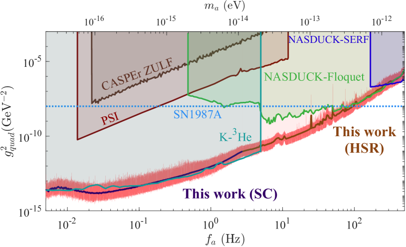
Figure 5: The 95% C.L. upper limits (depicted by red lines) for the quadratic coupling $g_{\rm quad}^{2}$ are derived from measurements in both the self-compensating (SC) and hybrid spin-resonance (HSR) regimes, using the same labels as in Fig. 4.

Other axion couplings. It is worth noting that beside the linear axion coupling to nucleus spin, there is also a possibility of a quadratic coupling to spins Olive:2007aj ; Pospelov:2012mt ; wu2019search ; Jiang:2021dby . The corresponding Hamiltonian can be expressed as:

$$\mathcal{H}_{quad}=g_{quad}^{2}\mathbf{\nabla}a^{2}\cdot\mathbf{\sigma}_{N}.$$ (9)

Assuming that the quadratic coupling dominates, we can use the same analysis as above to recast it as results on $g_{quad}$. These are presented in Fig. 5. As a result of the quadratic coupling, the range of axion frequencies is reduced by a factor of two compared to the linear coupling, resulting in a range of $[0.005,500]$ Hz. The limits surpass the astrophysical constraints by several orders of magnitude for $f_{a}\lesssim 150$  Hz. These results also surpass the earlier terrestrial experiments.

In the supplementary materials, we provide detailed descriptions of the experimental setup, the dynamics and responses of the hybrid strongly-coupled spin system. Finally, we present the details of the additional tests conducted on the 62 possible candidates to determine whether they have a dark matter origin.

Appendix A The Experimental Setup

As shown in Fig. S1, the experimental setup comprises a spherical cell with a 12 mm diameter that holds a small droplet of K and Rb metal, along with $70\%$ isotope-enriched ²¹Ne and N₂ gases. To prevent the spontaneous emission transition of alkali atoms in the excited state and the generation of resonant photons with random spin polarization, we used N₂ gas as a quenching gas. Additionally, ²¹Ne gas acted as a buffer gas to reduce the rapid wall-collision relaxation of alkali spins.

The glass cell is heated using an AC electric heater to maintain a temperature of approximately $200^{\rm o}$C. To reduce low-frequency magnetic noise generated by the heating current, the current in the electric heater is modulated at 200 kHz. Temperature regulation and stabilization are achieved using a PID controller. The AC electric heater is located inside a PEEK vacuum chamber with water-cooling. This design reduces heat dissipation and minimizes the impact of air convection on the pump and probe lights. Additionally, the water-cooled chamber helps lower the temperature of surrounding magnetic shields, thereby improving the magnetic noise performance.

The vacuum chamber is shielded against magnetic interference using five layers of $\mu$-metal and one layer of Mn-Zn ferrite, which exhibits low intrinsic magnetic noise at the level of fT/Hz^1/2. To compensate for any residual magnetic fields in the chamber, a triaxial coil with a capacity of several nT is utilized, and it is also used to manipulate the spin ensembles. Circularly polarized pump light is used to transversely polarize the entire vapor cell along the $\hat{z}$ axis, while linearly polarized probe light is used to measure the transverse component of Rb polarization along the $\hat{x}$ axis. The intensity of both pump and probe beams is stabilized using liquid crystal variable retarders (LCVR) that rely on closed-loop PID-controlled circuits. The probe light is modulated at 50 kHz using a photoelastic modulator (PEM) and then demodulated using a lock-in amplifier to isolate low-frequency noise.

Appendix B Dynamics of Hybrid Strong-coupling Spin-Resonance

The collective polarizations of alkali and noble-gas spins are described by ${\bf{P^{e}}}={\bf{\left<S_{e}\right>}}/S_{e}$ and ${\bf{P^{n}}}={\bf{\left<K_{n}\right>}}/K_{n}$, respectively. In this context, $\bf{S_{e}}$ represents the valence electron spin operator (with $S_{e}=1/2$) of the alkali atom, while $\bf{K_{n}}$ denotes the nuclear spin of the noble-gas atoms ($K=1/2$ for ³He and $K=3/2$ for ²¹Ne). The dynamics of these spins, which occupy the same volume (i.e., the glass cell), can be characterized by the Bloch equations, which couple the alkali electron spin polarization ${\bf{P^{e}}}$ with the noble-gas nuclear spin polarization ${\bf{P^{n}}}$ kornack2005nuclear .

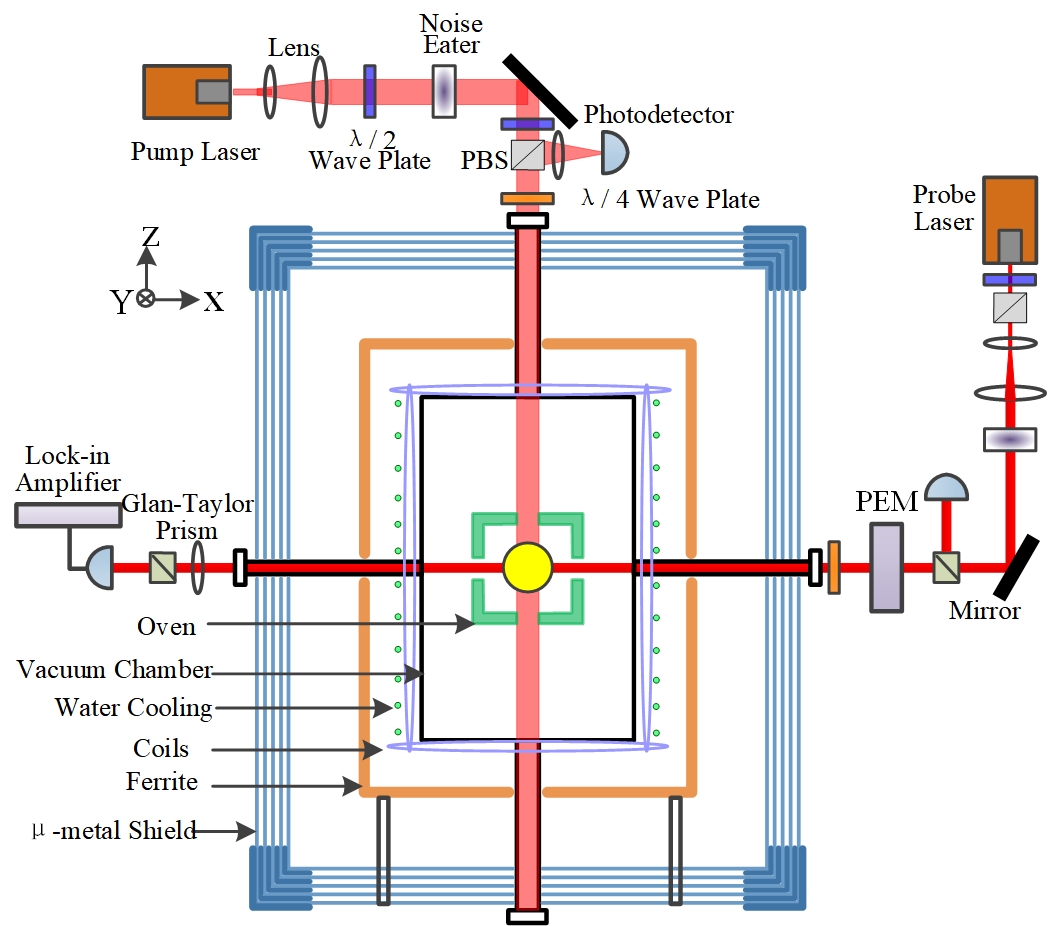
Figure S1: Basic principle of the hybrid strongly-coupled-spin system setup. At the center of the device is a glass cell containing a droplet of mixed K-Rb alkali metal, 3 amg ²¹Ne, 0.066 amg N₂, is installed in an oven, which is heated with an AC electric heater. The oven is enclosed in a plastic (PEEK) vacuum chamber to reduce the heat dissipation and air convection. The water cooled vacuum chamber also acts as the frame for triaxial magnetic coils. The vacuum chamber is enclosed in five layers of mu-metal magnetic shielding, and an inner Mn-Zn ferrite shield used to minimize the Johnson-current magnetic noise. The K atoms in the cell are spin polarized with circularly-polarized pump light propagating along $\hat{z}$. The Rb atoms are polarized by SE collisions with K atoms. The nuclear spins of ²¹Ne ($I=3/2$) are hyperpolarized via SE collisions with Rb atoms. The precession of ²¹Ne spins due to excitation, such as axion wind field, is transferred to Rb spins, which are coupled to ²¹Ne by the Fermi-contact interaction. The Rb atoms are probed with linearly-polarized light propagating along $\hat{x}$ via optical rotation. The probe light is polarization modulated with a photoelectric modulator (PEM) and demodulated with a lock-in amplifier to avoid the low-frequency noise. The pump and probe lasers are frequency- and amplitude stabilized (as described in Supplementary Information to wei2022constraints ). PBS, polarization beam splitter.

$$\frac{{\partial{{\bf{P}}^{\rm{e}}}}}{{\partial t}} =\frac{\gamma_{e}}{Q}\left({\bf{B}}+{\bf{\hat{B}^{\rm{n}}}}+{\bf{b}}^{\rm{e}}-{\Omega}\frac{Q_{e}}{\gamma_{e}}+{{\bf{L}}^{\rm{e}}}\right)\times{{\bf{P}}^{\rm{e}}}+\frac{R_{p}S^{P}_{z}+R^{\rm{ne}}_{\rm{se}}{{\bf{P}}^{n}}}{Q}{\bf{P}}^{\rm{e}}-\frac{\{{R^{e}_{1},R^{e}_{2},R^{e}_{2}}\}}{Q}{{{\bf{P}}^{e}}}+D_{e}\nabla^{2}{{\bf{P}}^{\rm{e}}},$$

$$\frac{{\partial{{{\bf{P}}^{\rm{n}}}}}}{\partial{t}} =\gamma_{n}\left({\bf{B}}+{\bf{\hat{B}^{\rm{e}}}}+{\bf{b}}^{\rm{n}}-\frac{\Omega}{\gamma_{n}}\right)\times{\bf{P}}^{\rm{n}}+R^{\rm{en}}_{\rm{se}}{{\bf{P}}^{e}}-{\{R^{n}_{1},R_{2}^{n},R_{2}^{n}\}}{{\bf{P}}^{\rm{n}}}+D_{n}\nabla^{2}{{\bf{P}}^{\rm{n}}}.$$ (S1)

The first equation describes the dynamics of alkali electron spins, while the second equation describes the dynamics of noble-gas nuclear spins. Each equation consists of four terms on the right-hand side. The first term describes the spin precession of the spin ensemble. Alkali electron spins precess under the sum of a classical magnetic field ${\bf{B}}$, an effective field ${\bf{\hat{B}^{n}}}$ from the noble-gas spins due to Fermi-contact interaction, an exotic field coupling to the electron spins due to ultralight dark matter ${\bf{b^{e}}}$, an inertial rotation $\Omega$, and an AC Stark light shift ${\bf{L^{e}}}$. Similarly, noble-gas spins precess under the sum of ${\bf{B}}$, an effective field ${\bf{\hat{B}^{e}}}$ from the alkali spins, an exotic field coupling to the nuclear spins due to ultralight dark matter ${\bf{b^{n}}}$, and $\Omega$. Here, $\gamma_{e}$ and $\gamma_{n}$ represent the gyromagnetic ratios of alkali electrons and noble-gas nuclei, respectively. The parameter $Q$ is the slowing-down factor of alkali atoms, which accounts for the influence of alkali nuclear spin.

The second term of each equation describes the spin polarization of alkali and noble-gas spins. Alkali spins are optically polarized using circularly polarized pump light at a pumping rate $R_{p}$, with photon spin $S^{p}_{z}\approx 1$. Additionally, alkali spins are polarized via spin-exchange collisions with noble-gas spins at a rate $R^{\rm{ne}}_{\rm{se}}$, which is negligible compared to the pumping rate $R_{p}$. Conversely, noble-gas spins are polarized via spin-exchange collisions with alkali spins at a rate $R^{\rm{en}}_{\rm{se}}$.

The third term of each equation describes the spin relaxation of the spin ensemble. The longitudinal and transverse spin components of alkali spins relax at rates $R^{e}_{1}$ and $R^{e}_{2}$, respectively, while the longitudinal and transverse spin components of noble-gas spins relax at rates $R^{n}_{1}$ and $R^{n}_{2}$, respectively. The final term of each equation characterizes the diffusion of each spin species, where $D_{e}$ and $D_{n}$ represent the diffusion constants of alkali and noble-gas atoms, respectively.

The Fermi contact interaction (FCI) between alkali and noble-gas spins can be described as an effective magnetic field that is observed by one spin species due to the magnetization of the other,

$${\bf{{\hat{B}}^{n/e}}}=\lambda M_{0}^{\rm{n/e}}{\bf{P^{n/e}}}\,.$$ (S2)

In this context, the effective field is magnified by a factor $\lambda$ when compared to the dipole field generated by the magnetization of each spin species. Here, $M_{0}^{e}$ and $M_{0}^{n}$ represent the magnetizations of alkali electrons and noble-gas nuclei, respectively, in the case of full polarization. The enhancement factor $\lambda$ is dependent on the geometry of the cell and the distribution of spin polarization. When the atomic cell is uniformly spin-polarized, the enhancement factor is given by $\lambda=2/3\kappa_{0}^{\rm{en}}$, where $\kappa_{0}^{\rm{en}}$ represents the FCI enhancement factor between alkali electron and noble-gas spins. For Rb-²¹Ne pair, $\kappa_{0}^{\rm{en}}=35.7$.

When a small transverse excitation is introduced, the longitudinal components of spin polarizations, $P^{e}_{z}$ and $P^{n}_{z}$, remain nearly unchanged and are equal to their respective equilibrium values, $P^{e}_{z0}=R_{p}S^{p}_{z}/R^{e}_{1}$ and $P^{n}_{z0}=P^{e}_{z0}R^{\rm{en}}_{\rm{se}}/R^{n}_{1}$. Therefore, the coupled Bloch equations can be linearized. To reduce the number of equations, the transverse components of alkali and noble-gas spins can be expressed as $P_{\bot}^{e}=P_{x}^{e}+iP_{y}^{e}$ and $P_{\bot}^{n}=P_{x}^{n}+iP_{y}^{n}$, respectively.

The dynamic response of the coupled alkali and noble-gas spin ensembles can be determined by solving the coupled Bloch equations. In this experiment, we measure the transverse component of alkali spins, $P^{e}_{x}(t)$, which can be expressed as:

$$P_{x}^{e}(t)=\rm{Re}[P_{1}\rm{exp}(-\Gamma_{e}t+\Omega_{e}t)+P_{2}\rm{exp}(-\Gamma_{n}t+\Omega_{n}t)]+P_{0}\,,$$ (S3)

where the two exponential terms correspond to the alkali and noble-gas spins, respectively. The parameters $\Gamma_{e}$ and $\Omega_{e}$ represent the decay rate and precession frequency of the alkali spins, while $\Gamma_{n}$ and $\Omega_{n}$ correspond to the noble-gas spins. The coefficients $P_{1}$, $P_{2}$, and $P_{0}$ are dependent on the specific working conditions. The decay rate and precession frequency of each spin species are interconnected with those of the other species, and can be expressed as:

$$\begin{split}\Gamma_{e}&=\frac{R_{2}^{e}/Q+R_{2}^{n}}{2}+\frac{1}{2\sqrt{2}}\sqrt{\sqrt{a^{2}+b^{2}}+a},\\ \Omega_{e}&=\frac{\omega^{e}_{z}+\omega^{n}_{z}}{2}-\frac{1}{2\sqrt{2}}\rm{Sign}(b)\sqrt{\sqrt{a^{2}+b^{2}}-a},\\ \Gamma_{n}&=\frac{R_{2}^{e}/Q+R_{2}^{n}}{2}-\frac{1}{2\sqrt{2}}\sqrt{\sqrt{a^{2}+b^{2}}+a},\\ \Omega_{n}&=\frac{\omega^{e}_{z}+\omega^{n}_{z}}{2}+\frac{1}{2\sqrt{2}}\rm{Sign}(b)\sqrt{\sqrt{a^{2}+b^{2}}-a}\,,\end{split}$$ (S4)

where the parameters $a$ and $b$ are given by

$$\begin{split}a={(R_{2}^{e}/Q-R_{2}^{n})^{2}}-{(\omega^{e}_{z}-\omega^{n}_{z})^{2}}+4R_{\rm{se}}^{\rm{ne}}/QR_{\rm{se}}^{\rm{en}}-4\omega^{\rm{ne}}_{z}\omega^{\rm{en}}_{z},\\ b=-2(R_{2}^{e}/Q-R_{2}^{n})(\omega^{e}_{z}-\omega^{n}_{z})-4(R_{\rm{se}}^{\rm{ne}}/Q\omega^{\rm{en}}_{z}+R_{\rm{se}}^{\rm{en}}\omega^{\rm{ne}}_{z})\,,\end{split}$$ (S5)

where $\omega^{e}_{z}=\gamma_{e}(\hat{B}^{n}_{z}+B_{z})/Q$, $\omega^{n}_{z}=\gamma_{n}(\hat{B}^{e}_{z}+B_{z})$, $\omega^{\rm{ne}}_{z}=\gamma_{e}\lambda M^{n}_{0}P^{e}_{z}/Q$, and $\omega^{\rm{en}}_{z}=\gamma_{n}\lambda M^{e}_{0}P^{n}_{z}$.

The coupling between alkali and noble-gas spins is determined by the dominant field $B_{z}$. When $B_{z}$ is much greater than $\hat{B}^{n}_{z}$, the alkali and noble-gas spin dynamics are decoupled. Under these conditions, the alkali spins decay and precess based on their own relaxation rate $R^{e}_{2}/Q$ and precession frequency $\gamma_{e}(B_{z}+\hat{B}^{n}_{z})/Q$, while noble-gas spins exhibit similar behavior, with a relaxation rate of $R^{n}_{2}$ and a precession frequency of $\gamma_{n}(B_{z}+\hat{B}^{e}_{z})$.

However, at the strongly-coupled point where $B_{z}\approx-\hat{B}^{n}_{z}$, alkali and noble-gas spins become strongly coupled. This leads to hybridization between noble-gas spins and alkali spins, resulting in the maximum decay and precession rates for noble-gas spins. Therefore, the hybrid strong-coupling spin-resonance technique can be employed to measure signals that are coupled to noble-gas nuclear spins with high bandwidth, which is approximately three orders of magnitude greater than that of a spin-based amplifier.

Appendix C Responses of Hybrid Strong-coupling Spin-Resonance

The responses to oscillation input signals along transverse direction can be obtained by solving the coupled Bloch equations. The measured transverse component of alkali spins is

$$\begin{split}P^{e}_{x}&={\rm Re}\left[{P_{\bot}^{1}e^{i\omega t}+P_{\bot}^{2}e^{-i\omega t}}\right],\\ P_{\bot}^{1}&=\frac{{\gamma_{e}P_{z}^{e}}}{2Q}\frac{{(B_{\bot}+b_{\bot}^{e}-Q\Omega_{\bot}/\gamma_{e})(\omega-iR_{2}^{n}-\omega_{z}^{n})-(B_{\bot}+b_{\bot}^{n}-\Omega_{\bot}/\gamma_{n})\hat{\omega}^{n}_{z}}}{{(i\omega+R_{2}^{e}/Q-i\omega_{z}^{e})(i\omega+R_{2}^{n}-i\omega_{z}^{n})-i\omega_{z}^{ne}(-R_{se}^{en}+i\omega_{z}^{\rm{en}})}},\\ P_{\bot}^{2}&=\frac{{\gamma_{e}P_{z}^{e}}}{2Q}\frac{{(B_{\bot}+b_{\bot}^{e}-Q\Omega_{\bot}/\gamma_{e})(-\omega-iR_{2}^{n}-\omega_{z}^{n})-(B_{\bot}+b_{\bot}^{n}-\Omega_{\bot}/\gamma_{n})\hat{\omega}^{n}_{z}}}{{(-i\omega+R_{2}^{e}/Q-i\omega_{z}^{e})(-i\omega+R_{2}^{n}-i\omega_{z}^{n})-i\omega_{z}^{\rm{ne}}(-R_{\rm{se}}^{\rm{en}}+i\omega_{z}^{\rm{en}})}},\\ \end{split}$$ (S6)

where $\omega$ is the frequency of the signal, $B_{\bot}=B_{x}+iB_{y}$, $\Omega_{\bot}=\Omega_{x}+i\Omega_{y}$, $b_{\bot}^{e}=b_{x}^{e}+ib_{y}^{e}$, $b_{\bot}^{n}=b_{x}^{n}+ib_{y}^{n}$, and $\hat{\omega}^{n}_{z}=\gamma_{n}\hat{B}^{n}_{z}$.

The response to oscillation magnetic field $B_{y}=B_{y0}\cos(\omega t)$ is

$$\begin{split}P^{e}_{x(B_{y})}&={K_{B_{y}}}B_{y0}\cos(\omega t+{\phi_{B_{y}}}),\\ K_{B_{y}}&\approx\frac{{\gamma_{e}P_{z}^{e}}}{Q}\frac{\omega}{{\left\{{{{\left({\omega_{z}^{\rm{nn}}\omega_{z}^{\rm{ee}}-{\omega^{2}}}\right)}^{2}}+{{\left({R_{2}^{e}/Q\omega}\right)}^{2}}}\right\}}^{1/2}},\\ \end{split}$$ (S7)

where $K_{B_{y}}$ is the scale factor and $\hat{\omega}^{e}_{z}=\gamma_{e}\hat{B}^{e}_{z}/Q$.

The response to oscillation exotic field coupled to noble-gas spins $b_{x}^{n}=b_{x0}^{n}\cos(\omega t)$ is

$$\begin{split}P^{e}_{x(b_{x}^{n})}&={K_{b_{x}^{n}}}b_{x0}^{n}\cos(\omega t+{\phi_{b_{x}^{n}}}),\\ K_{b_{x}^{n}}&\approx\frac{{\gamma_{e}P_{z}^{e}}}{Q}\frac{\omega_{z}^{\rm{nn}}}{{\left\{{{{\left({\omega_{z}^{\rm{nn}}\omega_{z}^{\rm{ee}}-{\omega^{2}}}\right)}^{2}}+{{\left({R_{2}^{e}/Q\omega}\right)}^{2}}}\right\}}^{1/2}}.\\ \end{split}$$ (S8)

The scale factors for magnetic field $B_{y}$ and exotic field $b_{x}^{n}$ have the following relation

$$K_{B_{y}}=K_{b_{x}^{n}}\omega/\omega_{z}^{\rm{nn}}.$$ (S9)

As a result, the response to oscillating magnetic fields can be used to calibrate the response to exotic fields, which is a conventional calibration method in atomic magnetometry.

Appendix D The post-analysis of the possible candidates

Table S1: This flowchart presents the discrimination process for 62 potential DM candidates based on their frequency. The first column displays the frequency of each candidate, while the second column illustrates the background-only model test result for a redundant measurement using an external magnetic field located far from the HSR region. In the third and fourth columns, the LLR test results for half of dataset 1 are presented for two equivalent time durations of 90 hr, denoted as 1A and 1B, respectively. The results of the LLR tests should be larger than $23.7$ to pass the $5\sigma$ threshold since no need for the look-elsewhere effect. The final column summarizes whether each candidate is confirmed to be a DM signal or not based on the results of the tests performed.

frequency[Hz]	off-HSR bkg	1A	1B	Final result	frequency[Hz]	off-HSR bkg	1A	1B	Final result
46.704996	2713	3.3 (2717)	0.7 (2717)	2717	81.504437	2713	0.9 (2717)	0.0 (2717)	2717
48.391586	2717	0.1 (2717)	46.6 (2713)	2717	81.722087	2713	2.3 (2717)	3.7 (2717)	2717
67.129321	2717	0.0 (2717)	51.9 (2713)	2717	81.754539	2713	0.0 (2717)	0.0 (2717)	2717
67.143839	2717	0.0 (2717)	63.6 (2713)	2717	81.841119	2713	0.2 (2717)	0.0 (2717)	2717
67.162956	2713	1.7 (2717)	61.1 (2713)	2717	97.660449	2717	35.9 (2713)	2.5 (2717)	2717
67.164261	2717	0.3 (2717)	58.9 (2713)	2717	134.141310	2713	143.1 (2713)	0.5 (2717)	2717
67.239592	2713	0.0 (2717)	61.1 (2713)	2717	134.248210	2713	98.1 (2713)	0.0 (2717)	2717
67.256066	2717	1.9 (2717)	71.6 (2713)	2717	134.451360	2717	106.1 (2713)	0.0 (2717)	2717
67.299372	2713	3.2 (2717)	54.1 (2713)	2717	134.454310	2713	87.6 (2713)	0.0 (2717)	2717
67.305285	2717	0.0 (2717)	66.5 (2713)	2717	134.459880	2713	148.7 (2713)	0.0 (2717)	2717
67.372806	2713	11.5 (2717)	59.7 (2713)	2717	137.940290	2717	74.1 (2713)	0.0 (2717)	2717
67.378668	2717	0.2 (2717)	70.1 (2713)	2717	138.303850	2713	39.4 (2713)	0.0 (2717)	2717
67.384759	2713	0.0 (2717)	53.7 (2713)	2717	140.709640	2713	76.1 (2713)	4.5 (2717)	2717
67.399959	2717	2.5 (2717)	65.7 (2713)	2717	140.717360	2713	73.8 (2713)	0.0 (2717)	2717
67.401895	2713	0.6 (2717)	71.8 (2713)	2717	140.733530	2713	169.9 (2713)	0.0 (2717)	2717
67.424104	2713	0.9 (2717)	53.1 (2713)	2717	140.736620	2717	81.8 (2713)	0.0 (2717)	2717
67.439142	2713	0.0 (2717)	86.6 (2713)	2717	140.791670	2717	143.3 (2713)	1.8 (2717)	2717
67.447232	2717	0.0 (2717)	63.9 (2713)	2717	140.794650	2713	68.7 (2713)	0.0 (2717)	2717
67.457887	2717	4.4 (2717)	75.2 (2713)	2717	141.246730	2717	120.5 (2713)	0.3 (2717)	2717
72.782530	2713	8.2 (2717)	11.2 (2717)	2717	141.701700	2713	125.1 (2713)	6.7 (2717)	2717
72.785297	2713	0.0 (2717)	10.7 (2717)	2717	141.952930	2717	68.8 (2713)	0.0 (2717)	2717
72.788802	2713	0.0 (2717)	24.4 (2713)	2717	142.624590	2713	95.9 (2713)	3.4 (2717)	2717
72.797656	2713	0.8 (2717)	24.0 (2713)	2717	142.729810	2717	51.9 (2713)	4.5 (2717)	2717
72.803745	2717	0.0 (2717)	24.7 (2713)	2717	143.372440	2713	70.6 (2713)	4.3 (2717)	2717
72.823120	2713	0.0 (2717)	23.4 (2717)	2717	143.969920	2713	57.0 (2713)	0.2 (2717)	2717
72.825273	2713	10.2 (2717)	16.0 (2717)	2717	157.812310	2713	0.0 (2717)	40.1 (2713)	2717
72.839546	2713	0.7 (2717)	32.0 (2713)	2717	159.152270	2713	88.1 (2713)	0.1 (2717)	2717
72.869210	2713	0.0 (2717)	27.0 (2713)	2717	161.744220	2717	53.2 (2713)	11.2 (2717)	2717
72.871118	2713	1.5 (2717)	25.6 (2713)	2717	186.715230	2717	19.5 (2717)	0.0 (2717)	2717
72.874196	2717	0.0 (2717)	34.7 (2713)	2717	188.360580	2713	1.0 (2717)	0.0 (2717)	2717
72.921797	2713	1.1 (2717)	34.1 (2713)	2717	363.317150	2717	9.6 (2717)	119.5 (2713)	2717

This section presents a reanalysis of the 62 frequencies to evaluate their potential as dark matter candidates. The frequency range of interest spans from 46.7 Hz to 363.3 Hz. To assess the plausibility of these frequencies as dark matter signals, we conducted redundant measurements using an external magnetic field located outside the HSR region. We focused on the 62 frequencies and examined their proximity to $f_{a}\pm 0.27{\rm mHz}$. We performed a statistical test to determine whether the background-only model at $f_{a}$ exhibited an excess of $5\sigma$. If such an excess was observed, we excluded the corresponding candidate as a potential dark matter signal, since signal amplification is not possible and the excess may result from systematic backgrounds. The results of this analysis are presented in the second column of Table LABEL:tab:DM-signal-crosscheck as the ”off-HSR bkg” test, which excludes some of the candidates.

To further investigate the remaining frequencies, we divided Dataset 1 into two equal parts, referred to as 1A and 1B, each with a duration of 90 hours. We calculated the ${\rm LLR}$ for these frequencies separately, and the results are shown in the third and fourth columns of Table LABEL:tab:DM-signal-crosscheck. Since the coherent time $\tau_{a}$ of these frequencies is much smaller than the 90-hour duration of each data set, the calculated ${\rm LLR}$ for stable dark matter signals should exceed 23.7 for both 1A and 1B, without the need to consider the look-elsewhere effect. However, our results demonstrate that none of the candidates exhibit behavior consistent with a stable dark matter signal in the two-stage test.

Therefore, in conjunction with the off-HSR background test, the two-stage test rejects the possibility of a dark matter signal for all 62 frequencies.

References

- (1) Essig, R. et al. Working group report: New light weakly coupled particles. In Snowmass 2013: Snowmass on the Mississippi (2013). eprint 1311.0029.
- (2) Zyla, P. A. et al. Review of Particle Physics. PTEP 2020, 083C01 (2020).
- (3) Duffy, L. D. & van Bibber, K. Axions as Dark Matter Particles. New J. Phys. 11, 105008 (2009). eprint 0904.3346.
- (4) Marsh, D. J. E. Axion Cosmology. Phys. Rept. 643, 1–79 (2016). eprint 1510.07633.
- (5) Peccei, R. D. & Quinn, H. R. CP Conservation in the Presence of Instantons. Phys. Rev. Lett. 38, 1440–1443 (1977).
- (6) Peccei, R. D. & Quinn, H. R. Constraints Imposed by CP Conservation in the Presence of Instantons. Phys. Rev. D 16, 1791–1797 (1977).
- (7) Weinberg, S. A New Light Boson? Phys. Rev. Lett. 40, 223–226 (1978).
- (8) Wilczek, F. Problem of Strong and Invariance in the Presence of Instantons. Phys. Rev. Lett. 40, 279–282 (1978).
- (9) Vafa, C. & Witten, E. Parity Conservation in QCD. Phys. Rev. Lett. 53, 535 (1984).
- (10) Golub, R. & Lamoreaux, K. Neutron electric dipole moment, ultracold neutrons and polarized He-3. Phys. Rept. 237, 1–62 (1994).
- (11) Raffelt, G. G. Astrophysical methods to constrain axions and other novel particle phenomena. Phys. Rept. 198, 1–113 (1990).
- (12) Graham, P. W., Irastorza, I. G., Lamoreaux, S. K., Lindner, A. & van Bibber, K. A. Experimental Searches for the Axion and Axion-Like Particles. Ann. Rev. Nucl. Part. Sci. 65, 485–514 (2015). eprint 1602.00039.
- (13) Safronova, M. S. et al. Search for New Physics with Atoms and Molecules. Rev. Mod. Phys. 90, 025008 (2018). eprint 1710.01833.
- (14) Wu, T. et al. Search for axionlike dark matter with a liquid-state nuclear spin comagnetometer. Phys. Rev. Lett. 122, 191302 (2019).
- (15) Bloch, I. M., Hochberg, Y., Kuflik, E. & Volansky, T. Axion-like relics: new constraints from old comagnetometer data. Journal of High Energy Physics 2020, 1–38 (2020).
- (16) Bloch, I. M. et al. Nasduck serf: New constraints on axion-like dark matter from a serf comagnetometer. arXiv preprint arXiv:2209.13588 (2022).
- (17) Bloch, I. M., Hochberg, Y., Kuflik, E. & Volansky, T. Axion-like Relics: New Constraints from Old Comagnetometer Data. JHEP 01, 167 (2020). eprint 1907.03767.
- (18) Lee, J., Lisanti, M., Terrano, W. A. & Romalis, M. Laboratory Constraints on the Neutron-Spin Coupling of feV-Scale Axions. Phys. Rev. X 13, 011050 (2023). eprint 2209.03289.
- (19) Jiang, M., Su, H., Garcon, A., Peng, X. & Budker, D. Search for axion-like dark matter with spin-based amplifiers. Nature Phys. 17, 1402–1407 (2021). eprint 2102.01448.
- (20) Carenza, P. et al. Improved axion emissivity from a supernova via nucleon-nucleon bremsstrahlung. JCAP 10, 016 (2019). [Erratum: JCAP 05, E01 (2020)], eprint 1906.11844.
- (21) Buschmann, M., Dessert, C., Foster, J. W., Long, A. J. & Safdi, B. R. Upper Limit on the QCD Axion Mass from Isolated Neutron Star Cooling. Phys. Rev. Lett. 128, 091102 (2022). eprint 2111.09892.
-
(22)
Lee, J.
New Constraints on the Axion’s Coupling to
Nucleons
from a Spin Mass Interaction Limiting Experiment (SMILE). Ph.D. thesis, Princeton University (2019). - (23) Babcock, E. et al. Hybrid spin-exchange optical pumping of h e 3. Physical review letters 91, 123003 (2003).
- (24) Romalis, M. Hybrid optical pumping of optically dense alkali-metal vapor without quenching gas. Physical review letters 105, 243001 (2010).
- (25) Not to be be confused with hybrid optical pumping.
- (26) Wei, K. et al. Constraints on exotic spin-velocity-dependent interactions. Nature Communications 13, 7387 (2022).
- (27) Wei, K. et al. Ultrasensitive Atomic Comagnetometer with Enhanced Nuclear Spin Coherence. Phys. Rev. Lett. 130, 063201 (2023). eprint 2210.09027.
- (28) Jiang, M., Su, H., Wu, Z., Peng, X. & Budker, D. Floquet maser. Sci. Adv. 7, eabe0719 (2021).
- (29) Kornack, T., Smullin, S., Lee, S.-K. & Romalis, M. A low-noise ferrite magnetic shield. Applied physics letters 90, 223501 (2007).
- (30) Kornack, T., Ghosh, R. & Romalis, M. Nuclear spin gyroscope based on an atomic comagnetometer. Phys. Rev. Lett. 95, 230801 (2005).
- (31) The data for axion coupling limits (2023). URL .
- (32) Bloch, I. M. et al. New constraints on axion-like dark matter using a Floquet quantum detector. Sci. Adv. 8, abl8919 (2022). eprint 2105.04603.
- (33) Abel, C. et al. Search for ultralight axion dark matter in a side-band analysis of a 199Hg free-spin precession signal (2022). eprint 2212.02403.
- (34) Bhusal, A., Houston, N. & Li, T. Searching for Solar Axions Using Data from the Sudbury Neutrino Observatory. Phys. Rev. Lett. 126, 091601 (2021). eprint 2004.02733.
- (35) Brown, B. A., Bertsch, G. F., Robledo, L. M., Romalis, M. V. & Zelevinsky, V. Nuclear Matrix Elements for Tests of Local Lorentz Invariance Violation. Phys. Rev. Lett. 119, 192504 (2017). eprint 1604.08187.
- (36) Almasi, A., Lee, J., Winarto, H., Smiciklas, M. & Romalis, M. V. New Limits on Anomalous Spin-Spin Interactions. Phys. Rev. Lett. 125, 201802 (2020). eprint 1811.03614.
- (37) Vasilakis, G., Brown, J., Kornack, T. & Romalis, M. Limits on new long range nuclear spin-dependent forces set with a k- he 3 comagnetometer. Physical review letters 103, 261801 (2009).
- (38) Brown, J., Smullin, S., Kornack, T. & Romalis, M. New limit on lorentz-and c p t-violating neutron spin interactions. Physical review letters 105, 151604 (2010).
- (39) Workman, R. L. et al. Review of Particle Physics. PTEP 2022, 083C01 (2022).
- (40) Beznogov, M. V., Rrapaj, E., Page, D. & Reddy, S. Constraints on Axion-like Particles and Nucleon Pairing in Dense Matter from the Hot Neutron Star in HESS J1731-347. Phys. Rev. C 98, 035802 (2018). eprint 1806.07991.
- (41) Di Luzio, L., Fedele, M., Giannotti, M., Mescia, F. & Nardi, E. Stellar evolution confronts axion models. JCAP 02, 035 (2022). eprint 2109.10368.
- (42) Chang, J. H., Essig, R. & McDermott, S. D. Supernova 1987A Constraints on Sub-GeV Dark Sectors, Millicharged Particles, the QCD Axion, and an Axion-like Particle. JHEP 09, 051 (2018). eprint 1803.00993.
- (43) Bar, N., Blum, K. & D’Amico, G. Is there a supernova bound on axions? Phys. Rev. D 101, 123025 (2020). eprint 1907.05020.
- (44) Masia-Roig, H. et al. Intensity interferometry for ultralight bosonic dark matter detection. arXiv preprint arXiv:2202.02645 (2022).
- (45) Bovy, J., Hogg, D. W. & Rix, H.-W. Galactic masers and the Milky Way circular velocity. Astrophys. J. 704, 1704–1709 (2009). eprint 0907.5423.
- (46) de Salas, P. F. & Widmark, A. Dark matter local density determination: recent observations and future prospects. Rept. Prog. Phys. 84, 104901 (2021). eprint 2012.11477.
- (47) Banerjee, A. et al. Searching for Earth/Solar Axion Halos. JHEP 09, 004 (2020). eprint 1912.04295.
- (48) Foster, J. W., Rodd, N. L. & Safdi, B. R. Revealing the Dark Matter Halo with Axion Direct Detection. Phys. Rev. D 97, 123006 (2018). eprint 1711.10489.
- (49) Centers, G. P. et al. Stochastic fluctuations of bosonic dark matter. Nature Commun. 12, 7321 (2021). eprint 1905.13650.
- (50) Lisanti, M., Moschella, M. & Terrano, W. Stochastic properties of ultralight scalar field gradients. Phys. Rev. D 104, 055037 (2021). eprint 2107.10260.
- (51) Gramolin, A. V. et al. Spectral signatures of axionlike dark matter. Phys. Rev. D 105, 035029 (2022). eprint 2107.11948.
- (52) Derevianko, A. Detecting dark-matter waves with a network of precision-measurement tools. Phys. Rev. A 97, 042506 (2018). eprint 1605.09717.
- (53) Terrano, W. & Romalis, M. Comagnetometer probes of dark matter and new physics. Quantum Science and Technology 7, 014001 (2021).
- (54) Lee, J., Lisanti, M., Terrano, W. A. & Romalis, M. Laboratory constraints on the neutron-spin coupling of fev-scale axions. arXiv preprint arXiv:2209.03289 (2022).
- (55) Vasilakis, G., Brown, J. M., Kornack, T. W. & Romalis, M. V. Limits on new long range nuclear spin-dependent forces set with a K - He-3 co-magnetometer. Phys. Rev. Lett. 103, 261801 (2009). eprint 0809.4700.
- (56) Olive, K. A. & Pospelov, M. Environmental dependence of masses and coupling constants. Phys. Rev. D 77, 043524 (2008). eprint 0709.3825.
- (57) Pospelov, M. et al. Detecting Domain Walls of Axionlike Models Using Terrestrial Experiments. Phys. Rev. Lett. 110, 021803 (2013). eprint 1205.6260.