The quantum geometric origin of capacitance in insulators

Abstract

In band insulators, where the Fermi surface is absent, adiabatic transport is allowed only due to the geometry of the Hilbert space. When the system is driven at a small but finite frequency $\omega$, transport is still expected to depend sensitively on the quantum geometry. Here we show that this expectation is correct and can be made precise by expressing the Kubo formula for conductivity as the variation of the time-dependent polarization with respect to the applied field. In particular, a little appreciated effect is that at linear order in frequency, the longitudinal conductivity results from an intrinsic capacitance, determined by the ratio of the quantum metric and the spectral gap. We demonstrate that this intrinsic capacitance has a measurable effect in a wide range of insulators with non-negligible metric, including the electron gas in a quantizing magnetic field, the gapped bands of hBN-aligned twisted bilayer graphene, and obstructed atomic insulators such as diamond whose large refractive index has a topological origin. We also discuss the influence of quantum geometry on the dielectric constant.

Introduction. — Historically, the primary focus when examining material properties has been the electronic band structure. However, following the transformative impact of the modern theory of polarization [1], the Hilbert space geometry has emerged in recent years as a critical instrument for characterizing quantum materials. This perspective shift has been fueled mainly by the rapid progress in the understanding of the quantum geometric tensor (QGT) [2], whose imaginary part, the Berry curvature, has become indispensable in addressing topological band structure properties [3, 4, 5]. On the other hand, the real part, known as the quantum metric has only recently attracted attention. This quantity was shown to appear in various transport functions [6, 7, 8, 9, 10], and may contribute to the superfluid stiffness in flatband superconductors [11, 12, 13, 14].

Here, we add to this growing list a seemingly overlooked property of the QGT, which is how it enters canonically in the quasistatic conductivity in insulators. This perspective is motivated by the modern theory of polarization: The polarization $P^{\mu}$ can be defined by carefully evaluating the position operator in momentum space [15, 16, 17]. This implies that $P^{\mu}$ is determined entirely by the eigenfunctions of a given Bloch-periodic Hamiltonian and independent of the eigenvalues (dispersion). Since the current can be defined as a derivative of the polarization $j^{\mu}=dP^{\mu}/dt$, it is tempting to seek similar conclusions for $j^{\mu}$. this expectation is indeed true for a band insulator, where the dc-current is purely transverse, dissipationless and proportional to the Chern number of the ground state.

Here, we investigate how the linear response in an insulator changes away from the zero-frequency limit, establishing that the quasistatic expansion for low frequencies contains valuable additional information about the quantum geometry of the Hilbert space. This insight allows us to connect the longitudinal conductivity with the quantum metric in insulators where the typical bandwidth is small compared to the band gap.

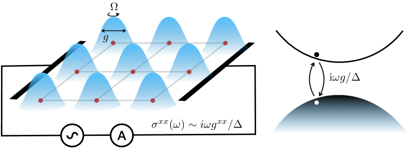
Figure 1: Emergence of the intrinsic capacitance in insulators with nonzero quantum metric $g$. Upon applying an ac electric field, due to virtual excitations a transient polarization is induced, which entails a longitudinal, purely imaginary impedance.

The starting point for our considerations is the static susceptibility $\chi$ in insulators expressed in terms of the polarization as $\chi^{\mu\nu}=\partial P^{\nu}/\partial E^{\mu}$ [1]. Using the definition of the current, one can similarly evaluate the conductivity as $\sigma^{\mu\nu}\to\partial j^{\nu}/\partial E^{\mu}$. However, since the current arises in a quasisteady state, it is not obvious to which extent the properties of a static polarization carry over to the conductivity [18, 16, 19]. We show by explicit construction using the Kubo formula that linear conductivity $\sigma$ in both insulators and metals can be expressed in terms of the polarization as

$$\sigma^{\mu\nu} =\frac{\delta}{\delta E^{\mu}(t)}\biggl{(}\frac{dP^{\nu}(t)}{dt}\biggr{)}\bigg{|}_{E^{\mu}=0}\,,$$ (1)

where the time dependence enters through the monochromatic electric field $E_{\mu}(t)=E_{\mu}e^{i\omega t}$. Eq. (1) makes use of a functional derivative with respect to the time-dependent field, which allows writing the conductivity in a deceptively simple manner, $\sigma^{\mu\nu}=\delta j^{\nu}/\delta E^{\mu}(t)$. Based on this insight, we are motivated to explore the geometric content of the quasistatic response. Focusing on two-dimensional insulators with rotational symmetry, the low-frequency expansion yields

$$\sigma^{\mu\nu}(\omega) =-\frac{e^{2}}{h}C\varepsilon^{\mu\nu}+i\omega c\,\delta^{\mu\nu}+\dots\,,$$ (2)

with the capacitance $c$ being related to the static susceptibility via the vacuum permittivity $\varepsilon_{0}$ as $c=\varepsilon_{0}\chi$, and $C$ denoting the Chern number. That is, the capacitance $c$ constitutes the leading low-frequency longitudinal contribution, indicative of the deviation from the static response. This raises two important questions: Does this quantity depend on the quantum geometry? And is $c$ a substantial contribution in quantum materials? This letter answers both questions with yes. In particular, we present several examples of non-interacting band insulators where the intrinsic capacitance $c$ contains the matrix elements of the quantum metric, normalized by the respective band gaps. The appearance of the quantum metric in the quasistatic conductivity can be understood intuitively by recalling that the quantum metric quantifies the extent of a wavefunction in real space [20, 19]. Therefore, it measures how much the electrons can polarize. In short, systems with a finite quantum metric exhibit an intrinsic capacitance. This capacitance is a purely quantum phenomenon that arises from coherent, virtual interband transitions between the full valence band and the empty conduction band [21], simply because within a full band quasiparticles cannot be displaced at all (cf. Fig. 1).

We emphasize that the intrinsic capacitance $c$ originates solely from the multi-banded nature of insulators, making it the only electronic contribution to the geometric capacitance of clean insulators at frequencies smaller than the band gap. In dirty or doped insulators, due to in-gap bound states [22] the measured capacitance is augmented by the quantum capacitance, which is proportional to the density of states at the Fermi level inside the mobility gap. As the trace of the quantum metric is bounded by the Chern number [23, 11, 24], we expect the capacitive response to be enhanced in systems where the orbitals cannot be exponentially localized. In the following, we clarify under which circumstances the intrinsic capacitance can be used as a diagnostics of the quantum geometry of the system.

Geometric expansion of the Kubo formula. — It is well established that in the adiabatic transport regime, the response of an insulator to external fields is dictated by the geometry of the Hilbert space. Eq. (1) indicates that beyond the adiabatic regime, we may view the conductivity solely as a geometric quantity in the Hilbert space slowly evolving in time. This statement is now made precise. To this end, let us consider a periodic system with Bloch wavefunctions $|m\bm{k}\rangle$ and energy eigenvalues $\hbar\omega_{m}(\bm{k})$, where $m$ is the band index, and in the following we will suppress the momentum index. Using the Kubo formula, we find that any response at finite frequency depends explicitly on the band dispersion of filled and empty bands. This dependence is introduced by the interband elements of the current operator $J_{nm}^{\mu}$ with spatial index $\mu$, which are explicitly given by $J_{nm}^{\mu}=ie(\omega_{m}-\omega_{n})r^{\mu}_{mn}\equiv ie\omega_{nm}r^{\mu}_{mn}$, with $r^{\mu}_{mn}=\langle m|\hat{r}^{\mu}|n\rangle$ representing the matrix elements of the position operator. In the insulating state, the conductivity exclusively depends on interband terms which are given by

$$\sigma^{\mu\nu}(\omega)=-\frac{ie^{2}}{\hbar}\sum\limits_{n\neq m}\int_{\rm BZ}f_{nm}\omega_{nm}\frac{r^{\mu}_{nm}r^{\nu}_{mn}}{\omega_{nm}+\omega}\,,$$ (3)

where we introduced the difference of occupation functions $f_{nm}=f_{n}-f_{m}$. The integral is over the Brillouin zone, and all band structure quantities implicitly depend on the momentum unless specified otherwise. As we further detail in the supplementary information [25], this expression can be exactly rewritten as

$$\sigma^{\mu\nu}(\omega)=-\frac{e^{2}}{\hbar}\int_{\rm BZ}\!\left(\Omega^{\mu\nu}\!-\omega\int_{\rm C}dt\,e^{-i\omega_{+}t}\,\hat{T}Q^{\mu\nu}(t)\right)$$ (4)

where we introduced a time-dependent QGT

$$Q^{\mu\nu}(t)=\sum\limits_{n\neq m}f_{n}(1-f_{m})r^{\mu}_{nm}(t)r^{\nu}_{mn}(0)\,.$$ (5)

Note that the integral in (4) is evaluated over the Keldysh contour $\rm C$ [25], and $\hat{T}$ denotes path ordering. $Q(t)$ can be written succinctly in operator form as $Q^{\mu\nu}(t)\equiv\mathrm{Tr}[\hat{P}\hat{r}^{\mu}(t)(1-\hat{P})\hat{r}^{\nu}(0)]$ [26], where $\hat{P}$ is the projector into the filled bands. In this form, the time-dependent QGT can be clearly identified as a generalization of the time-independent QGT.

The intrinsic capacitance arises in the Kubo formula upon expansion to linear order in the driving frequency. We assume that the frequency is well below the band gap, and therefore transport is non-dissipative. Let us concentrate on the longitudinal conductivity that in the absence of dissipation is purely imaginary. Expanding in powers of frequency $\sigma^{\mu\mu}\simeq i\omega c^{\mu\mu}+O(\omega^{3})$, we extract the capacitance

$$c^{\mu\mu}=\frac{2e^{2}}{\hbar}\int_{\rm BZ}\sum_{m\neq n}f_{n}(1-f_{m})\frac{g^{\mu\mu}_{mn}}{\omega_{mn}}\,,$$ (6)

where the numerator contains the matrix elements of the quantum metric $g^{\mu\mu}_{mn}=\{r^{\mu}_{nm},r^{\mu}_{mn}\}/2$, from which the full ground state quantum metric can be obtained by the summation $g^{\mu\mu}=\sum_{nm}f_{n}(1-f_{m})g_{mn}^{\mu\mu}$. For isotropic systems, we drop the spatial indices, such that $c\equiv c^{\mu\mu}$. The identification of an intrinsic capacitance due to the quantum metric, Eq. (6), is the main result of this work.

Landau Levels. — We first consider the intrinsic capacitance in the well-known case of an electron gas under an applied out of plane magnetic field $B$. The spectrum of this problem consists of flat Landau levels with a uniform gap given by the cyclotron frequency $\omega_{nm}=\omega_{c}=eB/m_{e}$. Since the dipole transitions are only allowed between neighboring Landau levels, i.e. $r^{\mu}_{nm}\propto\delta_{n,m+1}$, Eq. (6) simplifies dramatically. The quantum metric for the case of Landau levels is given by $g^{xx}=l_{\rm B}^{2}C$ [24] with $l_{\rm B}=\sqrt{\hbar/eB}$, such that the capacitance takes the quantized value of [25]

$$c=\frac{e^{2}}{h\omega_{c}}C\,.$$ (7)

Most importantly, this implies that at sufficiently small frequency, each filled Landau level carries a quantum of capacitance $c_{0}=e^{2}/h\omega_{c}$. The reason for that can be gleaned from Eq. (6): in a system with flatband dispersion, the energy difference $\omega_{mn}$ can be taken out of the momentum integral, such that only the integral over $g_{mn}$ remains. For a magnetic field of $1\,$T, we find $c_{0}\simeq 0.22\,\mathrm{fF}$, which is well within the range of Microwave Impedance Microscopy (MIM) devices [27, 28].

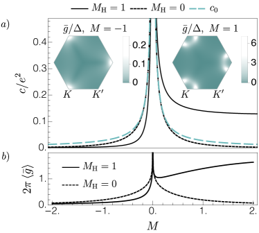
Figure 2: Relation between the quantum metric and intrinsic capacitance $c$ in a Haldane-like model compared against the linear Dirac cone result (9). $a)$ The top panel displays $c$ as a function of the mass parameter $M$. The solid curve corresponds to the value of the Haldane mass $M_{\rm H}=1$, while the black dashed curve represents $M_{\rm H}=0$. The colored dashed curve represents the capacitance $c_{0}$ of a linear Dirac cone. The insets on the left and right show the relative contributions to $c$ across the Brillouin zone in the Haldane $M_{\rm H}=1$ model with $M=-1$ and $M=1$, respectively. The involvement of the high-momentum modes for $M=1$ confirms the topological nature of transport in this parameter region. $b)$ Integrated, normalized, traced over the spatial indices quantum metric $\braket{\bar{g}}=\int_{\rm BZ}(g^{xx}+g^{yy})$ in the Haldane model with $M_{\rm H}=1$ (solid line), and for $M_{\rm H}=0$ (dashed line). Both $c$ and $\left<\bar{g}\right>$ for $M_{\rm H}=0$ are divided by a factor of two for better comparison, since in this case at $M=0$ the gap closes in both valleys.

Gapped Dirac Hamiltonians. — We consider a two-dimensional gapped Dirac dispersion, given by the continuum Hamiltonian $\hat{H}=k^{\mu}\hat{\sigma}_{\mu}+M\hat{\sigma}_{z}$. The longitudinal ac conductivity (3) simplifies to

$$\sigma(\omega)={ie^{2}\omega}\int_{\rm BZ}\frac{\Delta\bar{g}}{\Delta^{2}-(\hbar\omega)^{2}}\,,$$ (8)

with the gap given by $\Delta=2\sqrt{M^{2}+k^{2}}$ [25], and $\bar{g}=g^{xx}+g^{yy}$. For low frequencies, far smaller than the gap, the linear coefficient of $i\omega$ corresponds to the capacitance of a massive Dirac fermion

$$c_{0}=\frac{e^{2}}{12\pi|M|}\,.$$ (9)

This quantity approximates well the contribution to the capacitance per Dirac cone in topologically trivial materials. To consider the influence of topology on this value, we consider a Dirac Hamiltonian with a quadratic correction $\hat{H}^{\prime}=k^{\mu}\hat{\sigma}_{\mu}+(M-\alpha k^{2})\hat{\sigma}_{z}$, which yields for the capacitance

$$c_{0}^{\prime}=\begin{cases}\frac{e^{2}}{12\pi}\frac{1}{|M||1-4M\alpha|}\,,&\alpha M<0\,,\\ \frac{e^{2}}{12\pi|M|}+\frac{|\alpha|}{6\pi}\,,&\alpha M>0\,.\\ \end{cases}$$ (10)

If $M$ and $\alpha$ have the same sign, $\hat{H}^{\prime}$ describes a Chern insulator, with the capacitance acquiring a minimum value $c_{\rm min}=|\alpha|/6\pi$ in the limit $M\to\infty$. This behavior is reminiscent of the well-known bound on the quantum metric $2\pi\int_{\rm BZ}{\rm Tr}\,g\geq|C|$ [23, 11, 24]. In the trivial region $\alpha M<0$, $c_{0}^{\prime}$ decays faster than $c_{0}$. To summarize, the intrinsic capacitance diverges at a gap-closing, and acquires a characteristic asymmetry between trivial and topological phase, but only at a finite distance to the transition, while very close to the transition, $c_{0}^{\prime}\simeq c_{0}$ is symmetric.

To illustrate how these insights carry over to the tight-binding models of topological materials, we calculate the capacitance in a Haldane-like model parameterized by the sublattice staggered potential $M$, both with and without the Haldane mass term $M_{\rm H}$ [25]. As shown in Fig. 2, for finite $M_{\rm H}$, the system experiences a transition between the trivial phase ($M<0$) and the topological phase ($M>0$). As the gap closes at $M=0$, $c$ diverges on both sides of the phase transition. Close to the transition, $c$ is well approximated by the Dirac cone result $Nc_{0}$, where $N$ is the number of gapless valleys at $M=0$: $N=2$ for $M_{\rm H}=0$, and $N=1$ for $M_{\rm H}=1$. Similar to what we have demonstrated for $c_{0}^{\prime}$, the intrinsic capacitance is not symmetric across both phases: it saturates at a finite value on the topological side of the Haldane model but quickly decays to zero on the trivial side. In contrast, for zero Haldane mass ($M_{\rm H}=0$), $c$ remains symmetric deep into the gapped phase. These features of the intrinsic capacitance are due to its interband origin, which makes it sensitive both to geometric and topological properties of the band structure.

Magic angle twisted bilayer graphene — Let us now consider the magic-angle twisted bilayer graphene aligned on top of hBN [29, 30]. Due to the alignment, the in-plane inversion symmetry is broken, and the bands close to charge neutrality acquire a gap $\Delta$ of the order 10 meV [31]: this configuration makes the capacitance at half filling well-defined.

We calculate the capacitance $c$ numerically in the Bistritzer-MacDonald model [32] with a Fermi level at charge neutrality for realistic interlayer $AA$- and $AB$-sublattice tunneling parameters $u=0.077\,\rm eV$ and $u^{\prime}=0.11\,\rm eV$ [33]. The presence of the substrate is mimicked by a sublattice-polarized local term of strength $\Delta/2$. We are interested in the value of $c$ in a range of twist angles $\theta$ in the vicinity of the “magic” $\theta_{\rm M}\simeq 1.063^{\circ}$.

We present the resulting behavior of $c(\theta)$ in Fig. 3 for two values of $\Delta$. Since the dispersion in the flat bands is minimized at $\theta_{\rm M}$, based on Eq. (6) one would expect a local maximum of the capacitance to appear at the magic angle. Contrary to this expectation, this quantity develops instead a sharp local minimum since an abrupt decrease in the quantum metric of the flat bands around $\theta_{\rm M}$ dominates upon band flattening. The quench of the quantum metric due to the saturation of the trace condition is known to occur in the chiral limit of Bistritzer-MacDonald model [34] and expected to hold by continuity away from the $u\to 0$ limit. Interestingly, the value of the capacitance at the minimum can be roughly estimated as (9) multiplied by the number of Dirac quasiparticles, which for $\Delta=4\,$meV gives $8c_{0}\simeq 17\,{\rm aF}$.

We see that the behavior of the intrinsic capacitance $c$ correctly captures the distinctive and sudden decrease of the wavefunction spread that takes place when the bands are flattened, and therefore, the response $c$ emerges as an efficient probe of the quantum metric. We expect the suppression of the dielectric constant with ensuing anti-screening effects to play a role in stabilizing the interacting phases observed at the magic angle [35, 36]. We leave the investigation into the relevance of our findings to correlated phenomena for future work.

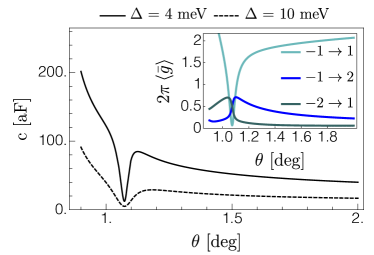
Figure 3: Intrinsic capacitance $c$ for hBN-aligned twisted bilayer graphene, depicted in relation to the twist angle $\theta$ for two values of the gap between the flat bands. In the inset, we sketch the behavior of the interband matrix elements of the quantum metric, integrated over the momentum in one valley for the case $\Delta=4\leavevmode\nobreak\ \rm meV$. The band indices are measured from charge neutrality, with $-1$ and 1 corresponding to the flat bands.

Electronic contribution to the dielectric constant — Having established the intrinsic capacitance as a valuable observable to diagnose the quantum geometry of systems with nearly flat bands, we address the question of what information $c$ contains in the case of generic insulators with dispersive spectrum. The (dimensionless) electronic component of the dielectric constant in linear response theory is given by $\epsilon^{\mu\nu}=\delta^{\mu\nu}+\chi^{\mu\nu}$, where the electric susceptiblity is [37]

$$\chi^{\mu\nu}=\frac{2e^{2}}{\hbar\varepsilon_{0}}\sum_{m\neq n}\int_{\rm BZ}f_{n}(1-f_{m})\frac{g^{\mu\nu}_{mn}}{\omega_{mn}}\,.$$ (11)

Since $\chi$ and $c$ are proportional, one may ask whether the localization properties of the electronic ground state can be extracted from the known values of the optical dielectric constant. With $\epsilon$ being a second rank tensor and using Eq. (11), one may in principle estimate any component of the quantum metric tensor $g$. For the sake of clarity, we will restrict the analysis to the in-plane component in materials with $C_{3}$ or $C_{4}$ rotational symmetry, where $\epsilon^{xx}=\epsilon^{yy}=\epsilon$ holds, with $\epsilon=1+\chi$.

To this end, we introduce the out-of-plane average of the in-plane quantum metric,

$$\langle\bar{g}\rangle_{z}=\int\frac{a_{z}dk_{z}}{2\pi}\int\frac{d^{2}{\bf k}}{(2\pi)^{2}}\,(g^{xx}+g^{yy})\,,$$ (12)

which is dimensionless, and $2\pi\langle\bar{g}\rangle_{z}$ can be directly compared with the Chern number. From the combination of Eq. (11) and Eq. (12), one can infer an approximate relation between $\langle\bar{g}\rangle_{z}$, the gap and the electric susceptibility

$${\langle\bar{g}\rangle_{z}}\sim\frac{\varepsilon_{0}a_{z}}{e^{2}}\chi\Delta.$$ (13)

By construction, in the limit where the band gap is large and the bands below and above the gap are nearly dispersionless, where (13) becomes a precise measure of the quantum metric.

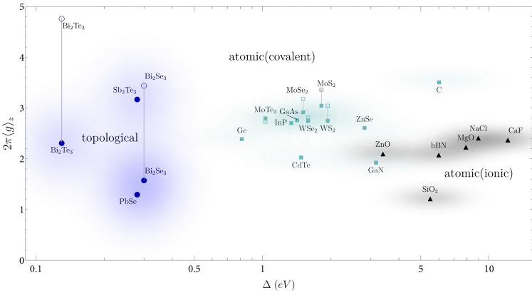
Figure 4: Estimate of the quantum metric $\left<\bar{g}\right>_{z}$ given in (13) as a function of the gap $\Delta$, according to Eqs. (12, 13). The $\left<\bar{g}\right>_{z}$ values computed from the experimental data are represented by full markers, and the theoretical calculations from the fitted tight-binding models are shown with open symbols. One can identify three main groups, distinguished by color: On the right (black), with a gap above $4\leavevmode\nobreak\ \rm eV$ and small metric, are the atomic insulators with ionic bonding, where the electrons predominantly surround an atomic site. In the middle (green), with a gap in the range $\sim 1-2\leavevmode\nobreak\ \rm eV$ are covalent insulators where electrons predominantly live on the bonds. Examples include transition metal dichalcogenide monolayers, $sp^{3}$ bonded semiconductors, and also the monoatomic obstructed atomic limits $\rm Si$ and $\rm Ge$, where the electrons cannot move from the bond due to symmetry constraints. On the left (blue) are topological insulators with narrow gaps ($\sim 0.2\leavevmode\nobreak\ \rm eV$). Although we expect the geometric contribution to be the largest in topological materials, we observe a sizeable discrepancy between the theoretical and experimental values of the susceptibility, which we associate with the existence of metallic surface states. Experimental values are according to [38, 39, 40, 41, 42, 64, 65, 66] and tabulated in the supplementary information.

In Fig. 4 we explore how well the relation (13) holds up for experimental values of $\chi$ and $\Delta$ (filled symbols) for a few topological and trivial materials with band gaps ranging from a few hundred meV to several eV. Quite intriguingly, we find values of $2\pi\langle\bar{g}\rangle_{z}$ across all materials, larger than 1, even in trivial ionic large gap insulators. However, we do observe important trends. Materials with large gaps, on the right of Fig. 4, are the atomic insulators with ionic bonding, whose electrons are well-bound to their original atoms, they show the lowest values of $\langle\bar{g}\rangle_{z}$. In the middle of Fig.4, we find covalent semiconductors, whose electrons live predominantly on the bonds. These include obstructed atomic limits (OALs) [43], where symmetry fixes the center of the electronic cloud in a high symmetry point such as the bond center. In these cases we find $\langle\bar{g}\rangle_{z}$ to be consistently higher than in ionic insulators. Intriguingly, a large number of transition metal dichalcogenides (TMDs), which are OALs [44], possess a quite similar $2\pi\langle\bar{g}\rangle_{z}\approx 2.8-3.0$. These values agree reasonably well with theoretical estimates of the quantum metric using tight-binding models [39] (empty symbols). On the left side of Fig. 4, at small energy gaps, we find strong topological insulators such as $\rm Bi_{2}Se_{3}$ and crystalline topological insulators such as $\rm PbSe$. These show an unexpectedly small $\langle\bar{g}\rangle_{z}$ when we estimate it from experimental values of $\chi$, and show large deviations from the estimated value obtained by a bulk tight-binding calculation, shown with open symbols. We attribute this discrepancy to the existence of metallic edge modes shown to dramatically alter the dielectric response of topological materials [45]. Let us also point out an interesting outlier, diamond ($\rm C$), which has a large gap, but nonetheless an atomic obstruction prevents electrons from localizing in the atomic sites but rather forces to be pinned by symmetry at the bonds, which leads to an abnormally high $\langle\bar{g}\rangle_{z}$ for the given value of the gap. This can be contrasted with $\rm GaN$, whose Wannier centers are situated close to the more electronegative element. The topological obstruction in diamond makes it a unique material with exceptionally large gap and high refractive index, which leads to its unique brilliance emanating from trapped refracted light.

Discussion. — We have explored the intimate connection between the quantum geometry and the low-frequency behavior encoded by Eq. (4) indicates that in insulators, not only the polarization but also the conductivity is completely determined by the properties of the Hilbert space, as long as the time evolution of the quantum geometric tensor is taken into account.

Based on this finding, we have shown for several examples how an estimate of the ground state quantum metric can be obtained by measuring the intrinsic capacitance. Specifically for TBG aligned with hBN, as a function of the twist angle we predict a sharp drop of the capacitance exactly at the magic angle, which is related to the corresponding decrease in the quantum metric. Compared to other measurement schemes for the quantum metric using the excitation rate of on-shell electronic transitions via sum rules [46, 47, 48, 49], the approach presented here does not require access to a wide frequency range.

Historically, the precise relation between the dielectric constant and the gap size in insulators has remained unclear, despite intense efforts [50, 51, 52, 53]. In light of this, the significance of Fig. 4 for the characterization of the dielectric properties of insulators is hard to overstate. As explained in detail, guided by our results for the quasistatic conductivity, we suggest the rescaling by the out-of-plane lattice constant before attempting a comparison of $\epsilon$ across materials, and conjecture that the remaining differences between materials with the same band gap but different $\chi$ are mostly due to the averaged quantum metric. While the relation presented in Eq. (13) clearly needs to be studied for more example cases, these assumptions seem to work well for bulk and layered $3D$ materials. Furthermore, we expect this approach to be useful in the search for new topological insulators, or for high refractive index materials.

A similar reformulation as the one demonstrated here might be possible for higher-order response functions, which can serve to illuminate the physical origin of the recently demonstrated corrections to the quantum anomalous Hall effect [54].

In this supplementary information, we present a detailed derivation of the relation between interband and intraband conductivity (Sec. A), quantum geometry (Sec. B), and the dynamical polarization (Sec. C). We apply the obtained relations to various example systems: namely, we present in detail how the time-dependent polarization enters in Landau levels (Sec. D), derive the quantum geometric tensor for Landau levels (Sec. E), and develop some intuition behind these findings by comparing them with a semiclassical point of view (Sec. F). This is followed by a derivation of the capacitance in a gapped Dirac cone model (Sec. G). Lastly, we present the complete data which was used to generate Figure 4 of the main text (Sec. H).

Appendix A Interband and intraband conductivity

In this section, we demonstrate how the Kubo formula for conductivity [55] can be split into intraband and interband terms. The former describes the conventional dissipative Fermi-surface transport, whereas the latter arises due to transitions between different bands. The starting point is the standard expression for the conductivity tensor (cf. e. g. [56]):

$$\sigma^{\mu\nu}(\omega)=\frac{i\bar{n}e^{2}}{m\omega_{+}}\delta^{\mu\nu}+\frac{1}{\hbar\omega_{+}A}\int_{0}^{\infty}dt\,e^{i\omega_{+}t}\braket{[\hat{J}^{\mu}(t),\hat{J}^{\nu}(0)]}\,,$$ (14)

where $\bar{n}$ is the total charge carrier density, $m$ and $e$ are the mass and the charge of the carriers, and $A$ is the area of the conducting sample. The brackets $\braket{\ldots}$ denote the vacuum expectation value. The convergence of the integral is ensured by an infinitesimal relaxation rate, i. e. $\omega_{+}=\omega+i\varepsilon$, $\varepsilon>0$. Henceforth, we mostly omit the subscript $+$, restoring it only where necessary to prevent singular behavior.

By inserting the complete basis of energy eigenstates $\ket{m{\bf k}}$, we write the commutator in Eq. (14) as

$$\braket{[\hat{J}^{\mu}(t),\hat{J}^{\nu}(0)]}=\sum\limits_{nm}\int_{\rm BZ}\frac{A\,d^{2}{\bf k}}{(2\pi)^{2}}f_{nm}({\bf k})\braket{n{\bf k}}{\hat{J}^{\mu}}{m{\bf k}}\braket{m{\bf k}}{\hat{J}^{\nu}}{n{\bf k}}e^{i\omega_{nm}({\bf k})t}\,,$$ (15)

where the indices $m$ and $n$ enumerate the bands, $\omega_{nm}\equiv\omega_{n}-\omega_{m}$, and $f_{nm}\equiv f_{n}-f_{m}$, where $f_{n}({\bf k})=\theta(E_{F}-\hbar\omega_{n}({\bf k}))$ is the zero temperature Fermi-Dirac distribution function with respect to the Fermi energy $E_{F}$. The matrix elements of the current operators are evaluated in the basis of Bloch states $\ket{n{\bf k}}=u_{n}({\bf k})\ket{{\bf k}}$, where $u_{n}({\bf k})$ are the eigenstates of the Hamiltonian in the momentum space: $\hat{H}({\bf k})u_{n}({\bf k})=\hbar\omega_{n}({\bf k})u_{n}({\bf k})$. In the following, we omit the momentum index and likewise use the shorthand notation

$$\int_{\rm BZ}\equiv\int_{\rm BZ}\frac{d^{2}{\bf k}}{(2\pi)^{2}}\,.$$ (16)

Plugging (15) into (14) and evaluating the time-integral, we obtain

$$\sigma^{\mu\nu}(\omega)=-\frac{i}{\hbar}\sum\limits_{nm}\int_{\rm BZ}\frac{f_{nm}}{\omega_{nm}}\frac{J^{\mu}_{nm}J^{\nu}_{mn}}{\omega_{nm}+\omega}\,,$$ (17)

where the first (diamagnetic) term in (14) was used to subtract the singular in $\omega\to 0$ limit piece in the commutator term. The remaining sum in Eq. (17) can be split into two contributions: The intraband part with $m=n$ and the interband part where $m\neq n$. The intraband conductivity is obtained from (17) by substituting

$$f_{nm} \to f\left(E_{F}-E_{n}({\bf k}+{\bf q})\right)-f\left(E_{F}-E_{n}({\bf k})\right)\,,$$ (18)

$$\omega_{nm} \to\omega_{n}({\bf k}+{\bf q})-\omega_{n}({\bf k})\,,$$

and taking a limit ${\bf q}\to 0$

$$\sigma_{\rm intraband}^{\mu\nu}(\omega)=\frac{i}{\omega}\sum\limits_{n}\int_{\rm BZ}f^{\prime}_{n}J^{\mu}_{nn}J^{\nu}_{nn}\,.$$ (19)

At zero temperature, the derivative of the Fermi function is simply a delta function $\delta(E_{F}-\hbar\omega_{n})$ that selects all the points in the BZ where the bands cross the Fermi surface. Hence, this contribution vanishes in insulators in the absence of disorder.

The interband ($m\neq n$) contribution to the sum (17) is convenient to express in terms of the position operators to make an explicit connection with quantum geometric quantities such as Berry curvature and quantum metric. In order to do so, we utilize

$$J^{\mu}_{nm}=\frac{e}{\hbar}\braket{n}{\partial^{\mu}\hat{H}}{m} =\frac{e}{\hbar}\bra{n}\partial^{\mu}\left(\hat{H}\ket{m}\right)-\frac{e}{\hbar}\bra{n}\hat{H}\ket{\partial^{\mu}m}$$ (20)

$$=\frac{e}{\hbar}(E_{m}-E_{n})\braket{n}{\partial^{\mu}m}=-ie\omega_{nm}r_{nm}^{\mu}\,.$$

Upon using $J^{\mu}_{nm}=-ie\omega_{nm}r^{\mu}_{nm}$, the interband contribution becomes

$$\sigma^{\mu\nu}_{\rm interband}(\omega)=-\frac{ie^{2}}{\hbar}\sum\limits_{n\neq m}\int_{\rm BZ}f_{nm}\omega_{nm}\frac{r^{\mu}_{nm}r^{\nu}_{mn}}{\omega_{nm}+\omega}\,.$$ (21)

The above term does not vanish in insulators even at zero frequency. For example, in the limit $\omega\to 0$ the expression above takes the form of the celebrated TKNN formula [57]

$$\sigma^{\mu\nu}_{\rm interband}(0) =-\frac{ie^{2}}{\hbar}\sum\limits_{n\neq m}\int_{\rm BZ}(f_{n}-f_{m})r^{\mu}_{nm}r^{\nu}_{mn}=-\frac{ie^{2}}{\hbar}\sum\limits_{n,m}\int_{\rm BZ}f_{n}(r^{\mu}_{nm}r^{\nu}_{mn}-r^{\nu}_{nm}r^{\mu}_{mn})$$ (22)

$$=-\frac{ie^{2}}{\hbar}\sum\limits_{n}\int_{\rm BZ}f_{n}(\braket{n}{\hat{r}^{\mu}\hat{r}^{\nu}}{n}-\braket{n}{\hat{r}^{\nu}\hat{r}^{\mu}}{n})=-\frac{ie^{2}}{\hbar}\sum\limits_{n}\int_{\rm BZ}f_{n}(\braket{\partial^{\mu}n}{\partial^{\nu}n}-\braket{\partial^{\nu}n}{\partial^{\mu}n})\,,$$

i.e. the conductivity is, up to a constant, the sum of the Chern numbers of the occupied bands. At non-zero frequency, on the other hand, it is not obvious that the interband contribution (21) is geometric in its origin: something one would expect to be the case in an insulator, at least in the small $\omega$ regime. To investigate this, one may further write:

$$\sigma^{\mu\nu}_{\rm interband}(\omega)=-\frac{ie^{2}}{\hbar}\sum\limits_{n\neq m}\int_{\rm BZ} \left[f_{n}(1-f_{m})-f_{m}(1-f_{n})\right]\,\omega_{nm}\frac{r^{\mu}_{nm}r^{\nu}_{mn}}{\omega_{nm}+\omega}$$ (23)

$$=-\frac{ie^{2}}{\hbar}\sum\limits_{n\neq m}\int_{\rm BZ}f_{n}(1-f_{m})\,\omega_{nm}\left(\frac{r^{\mu}_{nm}r^{\nu}_{mn}}{\omega_{nm}+\omega}-\frac{r^{\nu}_{nm}r^{\mu}_{mn}}{\omega_{nm}-\omega}\right)\,,$$

where we relabeled the summation indices in the second line. One may proceed by introducing the interband matrix elements of the Berry curvature and the quantum metric

$$\Omega_{nm}^{\mu\nu}=i(r^{\mu}_{nm}r^{\nu}_{mn}-r^{\nu}_{nm}r^{\mu}_{mn})\,,\qquad g_{nm}^{\mu\nu}=\frac{1}{2}(r^{\mu}_{nm}r^{\nu}_{mn}+r^{\nu}_{nm}r^{\mu}_{mn})\,.$$ (24)

With the definitions above, interband conductivity reads

$$\sigma^{\mu\nu}_{\rm interband}(\omega)=\frac{2ie^{2}}{\hbar}\sum\limits_{n\neq m}\int_{\rm BZ}f_{n}(1-f_{m})\frac{\omega\omega_{mn}}{\omega_{mn}^{2}-\omega^{2}}g^{\mu\nu}_{nm}-\frac{e^{2}}{\hbar}\sum\limits_{n\neq m}\int_{\rm BZ}f_{n}(1-f_{m})\frac{\omega_{mn}^{2}}{\omega_{mn}^{2}-\omega^{2}}\Omega^{\mu\nu}_{nm}\,.$$ (25)

Note that the second term never contributes to the longitudinal conductivity, since $\Omega_{nm}^{\mu\nu}$ is antisymmetric tensor. The metric $g_{nm}^{\mu\nu}$, on the other hand, may have off-diagonal components and contributes to $\sigma^{xy}(\omega)$. As we can see, the dispersion-dependent factors in the expression above prevent us from re-summing all the interband transitions into the integrals of the ground state quantities: Berry curvature and quantum metric

$$\Omega^{\mu\nu}=i\sum\limits_{n\neq m}f_{n}(1-f_{m})(r^{\mu}_{nm}r^{\nu}_{mn}-r^{\nu}_{nm}r^{\mu}_{mn})\,,\qquad g^{\mu\nu}=\frac{1}{2}\sum\limits_{n\neq m}f_{n}(1-f_{m})\left(r^{\mu}_{nm}r^{\nu}_{mn}+r^{\nu}_{nm}r^{\mu}_{mn}\right)\,.$$ (26)

This is a consequence of the non-adiabaticity introduced by the presence of $\omega$. Nevertheless, it does not mean that the interband contribution (21) is not purely quantum-geometric. As we will show explicitly in the next section, by considering the geometry of wavefunctions in space-time (${\bf k}$, $t$), one is able to express (21) solely in terms of the Hilbert space quantities.

Appendix B Time-dependent quantum geometric tensor

In clean insulators, with a finite excitation gap, quasiparticle transport is impossible, and one would not expect the dispersion to enter the response functions. It implies that the factors of $\omega_{nm}$ in (21) can be absorbed into the wavefunctions. Below we show that it is indeed the case and can be done by taking the time dependence of states (or operators) into account. We start with the expression (23)

$$\sigma^{\mu\nu}_{\rm interband}(\omega)=-\frac{ie^{2}}{\hbar}\sum\limits_{n\neq m}\int_{\rm BZ}f_{n}(1-f_{m})\,\omega_{nm}\left(\frac{r^{\mu}_{nm}r^{\nu}_{mn}}{\omega_{nm}+\omega}-\frac{r^{\nu}_{nm}r^{\mu}_{mn}}{\omega_{nm}-\omega}\right)\,.$$ (27)

We further decompose

$$\frac{\omega_{nm}}{\omega_{nm}+\omega}=1-\frac{\omega}{\omega_{nm}+\omega}\,,\qquad\frac{\omega_{nm}}{\omega_{nm}-\omega}=1+\frac{\omega}{\omega_{nm}-\omega}\,,$$ (28)

which yields

$$\sigma^{\mu\nu}_{\rm interband}(\omega)=-\frac{e^{2}}{\hbar}\int_{\rm BZ}\Omega_{\mu\nu}+\frac{ie^{2}\omega}{\hbar}\sum\limits_{n\neq m}\int_{\rm BZ}f_{n}(1-f_{m})\left(\frac{r^{\mu}_{mn}r^{\nu}_{nm}}{\omega_{nm}+\omega}-\frac{r^{\nu}_{mn}r^{\mu}_{nm}}{\omega_{mn}+\omega}\right)\,.$$ (29)

Reinstating the infinitesimal imaginary part of the frequency $\omega\to\omega_{+}$ to enforce convergence, and using the Schwinger representation

$$\frac{i}{\omega_{nm}+\omega_{+}}=\int_{-\infty}^{0}dt\,e^{-i(\omega_{nm}+\omega_{+})t}\,,$$ (30)

one can show that the terms with propagators in (29) can be conveniently wrapped up as

$$\quad\frac{e^{2}\omega}{\hbar}\sum\limits_{n\neq m}\int_{\rm BZ}f_{n}(1-f_{m})\left(\int_{-\infty}^{0}dt\,e^{-i(\omega_{nm}+\omega_{+})t}r^{\mu}_{mn}r^{\nu}_{nm}-\int_{-\infty}^{0}dt\,e^{-i(\omega_{mn}+\omega_{+})t}r^{\nu}_{mn}r^{\mu}_{nm}\right)$$ (31)

$$=\frac{e^{2}\omega}{\hbar}\sum\limits_{n\neq m}\int_{\rm BZ}f_{n}(1-f_{m})\left(\int_{-\infty}^{0}dt\,e^{-i\omega_{+}t}r^{\mu}_{mn}(t)r^{\nu}_{nm}+\int_{0}^{-\infty}dt\,e^{-i\omega_{+}t}r^{\nu}_{mn}r^{\mu}_{nm}(t)\right)$$ (32)

$$=\frac{e^{2}\omega}{\hbar}\int_{\rm C}dt\int_{\rm BZ}e^{-i\omega_{+}t}\,\hat{T}Q^{\mu\nu}(t)\,,$$ (33)

where the integral is taken over the Keldysh contour C sketched in Figure 1, $\hat{T}$ denotes the (advanced) ordering of operators along $\rm C$, and we introduced the time-dependent “quantum geometric tensor”

$$Q^{\mu\nu}(t)\equiv{\rm Tr}\left[\hat{P}\hat{r}^{\mu}(t)(1-\hat{P})\hat{r}^{\nu}(0)\right]\,,$$ (34)

where the operators appearing without the time label are taken at the initial time $t=0$, and the trace runs over band indices. The interband contribution to the Kubo formula for conductivity therefore assumes the form

$$\sigma^{\mu\nu}_{\rm interband}(\omega)=-\frac{e^{2}}{\hbar}\int_{\rm BZ}\left(\Omega^{\mu\nu}-\omega\int_{\rm C}dt\,e^{-i\omega_{+}t}\,\hat{T}Q^{\mu\nu}(t)\right)\,.$$ (35)

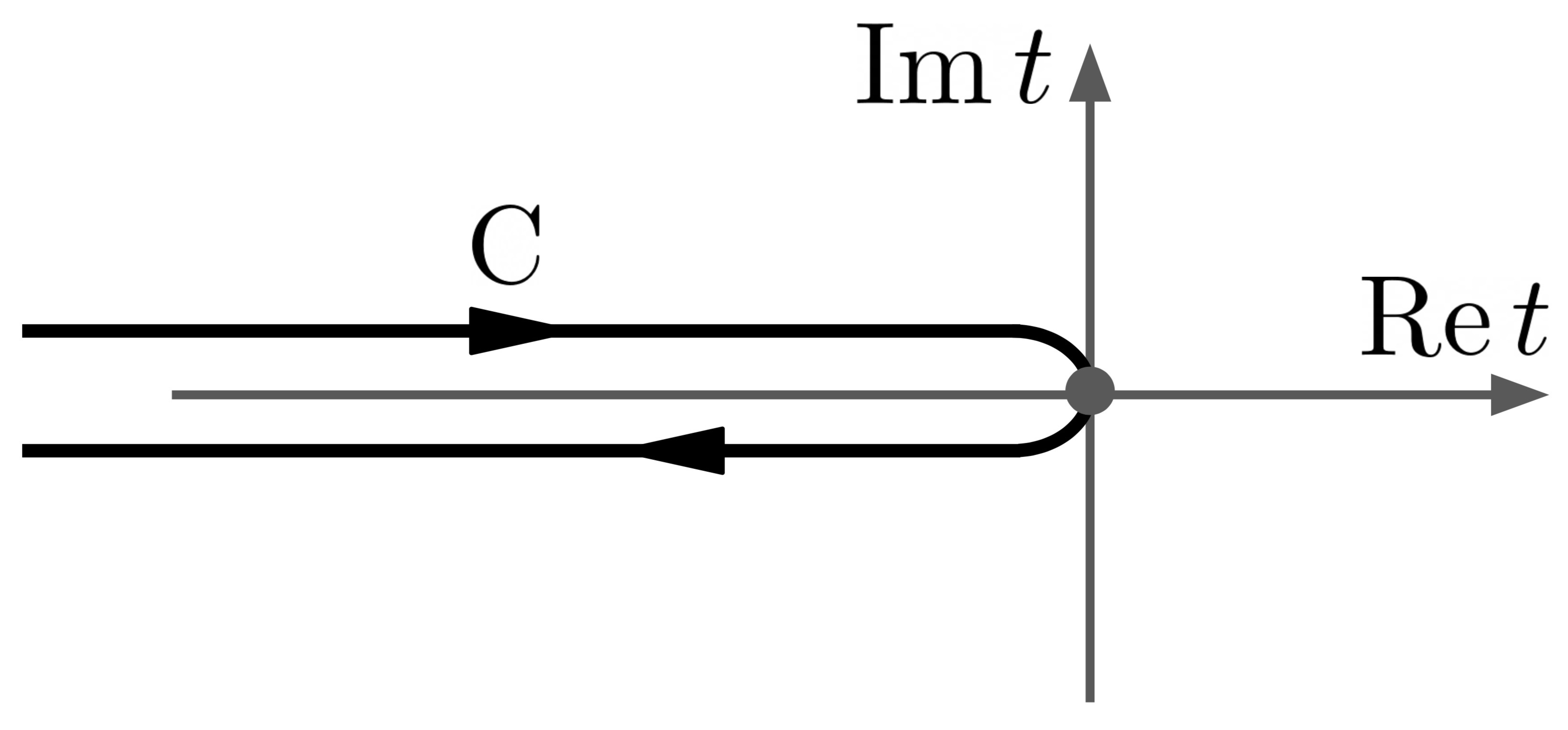
Supplementary Figure 1: Keldysh contour in complex time. The point at the axes crossing corresponds to $t=0$.

Since by definition $\Omega^{\mu\nu}=-2\,{\rm Im}\,Q^{\mu\nu}(t=0)$, the time-dependent quantity $Q^{\mu\nu}(t)$ solely determines the interband part of the conductivity, as a function of the time-dependent quantum geometry. For example, in the case of Landau levels, we have $\hat{r}^{\mu}(t)=\hat{r}^{\mu}e^{-i\omega_{c}t}$, and $Q^{\mu\nu}(t)=Q^{\mu\nu}e^{-i\omega_{c}t}$, and the momentum integral is taken over the reciprocal magnetic unit cell of the measure $2\pi/l_{\rm B}^{2}$. Plugging these expressions into Eq. (35), one obtains the ac conductivity tensor for Landau levels, Eq. (62). Hence, as proposed, the conductivity in insulators is entirely determined by the geometry of the Hilbert space.

Surprisingly, it turns out that not only the interband term allows for the geometric interpretation. In the next section, we take this reasoning one step further and show that the entire Kubo formula, including the intraband part, follows from the expectation value of the time-dependent position operator.

Appendix C Kubo formula for conductivity as a derivative of the polarization

In this section, we demonstrate that the schematic expression inspired by the modern theory of polarization [58]

$$\sigma^{\mu\nu}=\frac{\delta}{\delta E_{\mu}(t)}j^{\nu}(t)=\frac{\delta}{\delta E_{\mu}(t)}\frac{d}{dt}\left<P^{\nu}(t)\right>\,,$$ (36)

is not merely a convenient symbolic way of introducing electrical conductivity. On the other hand, quite literally, (36) is the Kubo formula for conductivity. In order to show it, we write

$$\sigma^{\mu\nu}=\frac{\delta}{\delta E_{\mu}(t)}\frac{d}{dt}\left<\frac{-e\hat{r}^{\nu}(t)}{A}\right>=-\frac{i\omega}{A}\frac{\delta}{\delta E_{\mu}(t)}\left<e\hat{r}^{\nu}(t)\right>\,,$$ (37)

where the expectation value of the time-dependent position operator in the Heisenberg picture is obtained via the Schwinger-Keldysh formalism with the interaction Hamiltonian (note the second term required by hermiticity)

$$H_{\rm int}=J_{\mu}A_{\mu}=\frac{i}{\omega}J_{\mu}E_{\mu}e^{i\omega t}-\frac{i}{\omega}J_{\mu}E_{\mu}e^{-i\omega t}\,.$$ (38)

The vacuum expectation value of the position operator at time $t$ is then

$$\frac{1}{A}\sum\limits_{n}\int_{\rm BZ}f_{n}\braket{n}{e\hat{r}^{\nu}(t)}{n}=\sum\limits_{n}\int_{\rm BZ}f_{n} \bra{n}\left(1+\frac{1}{\hbar\omega}\int_{-\infty}^{t}{\rm d}t^{\prime}\,e^{i\omega t^{\prime}}\hat{J}^{\mu}_{I}(t^{\prime})E_{\mu}\right)(e\hat{r}^{\nu}_{I}(t))\times$$ (39)

$$\qquad\qquad\qquad\times\left(1+\frac{1}{\hbar\omega}\int_{-\infty}^{t}{\rm d}t^{\prime}\,e^{i\omega t^{\prime}}\hat{J}^{\mu}_{I}(t^{\prime})E_{\mu}\right)\ket{n}+{\rm c.c.}+O(E^{2})\,,$$

where the subscript $I$ stands for the interaction picture with operators enjoying the “unperturbed” time-dependence $\hat{A}_{mn,I}(t)=e^{-i\omega_{mn}t}\hat{A}_{I}(0)$: in the following, to shorten the notation, we drop the subscript $I$. The expression c.c. stands for “complex conjugate” and contains the group of terms that oscillate with the frequency $e^{-i\omega t}$, which will be eliminated by the functional derivative $\delta/\delta E(t)$.

The $O(E^{0})$ term in the expression (39) is related to the net Berry phase of the occupied bands

$$ie\hbar\sum\limits_{n}\int_{\rm BZ}f_{n}\braket{n}{\partial^{\mu}n}\,.$$ (40)

It corresponds to the ferroelectric polarization that material possesses in the absence of an external electric field. The remaining terms represent the dielectric response: the fluctuation of the electric dipole moment under the influence of the external field. We further omit the $O(E^{2})$ terms that contain the information about the non-linear response: whether they reproduce the known non-linear contributions to conductivity is an interesting question that we leave for future work.

Keeping only the terms linear in $E_{\nu}$, inserting another sum over energy eigenstates $\sum_{n}\ket{m}\bra{m}$, and evaluating the time integrals, we write

$$\frac{1}{A}\left(\frac{\delta}{\delta E_{\mu}(t)}\braket{e\hat{r}^{\nu}(t)}\right)=\frac{ie}{\hbar\omega}\sum\limits_{mn}\int_{\rm BZ}\,f_{n}\left(\frac{J^{\mu}_{nm}r^{\nu}_{mn}}{\omega_{nm}+\omega}-\frac{r^{\nu}_{nm}J^{\mu}_{mn}}{\omega_{nm}-\omega}\right)\,.$$ (41)

We then interchange the summation indices in the second bracket:

$$-\frac{i\omega}{A}\left(\frac{\delta}{\delta E_{\mu}}\braket{e\hat{r}^{\nu}(t)}\right)=\frac{e}{\hbar}\sum\limits_{mn}\int_{\rm BZ}\,\left(f_{n}-f_{m}\right)\frac{J^{\mu}_{nm}r^{\nu}_{mn}}{\omega_{nm}+\omega}\,.$$ (42)

As soon as $m$ and $n$ are different, we are formally allowed to plug in $J^{\nu}_{nm}\to-ie\omega_{nm}r^{\nu}_{nm}$, so we arrive at the interband piece of the Kubo formula (21) :

$$\sigma^{\mu\nu}_{\rm interband}(\omega)=-\frac{ie^{2}}{\hbar}\sum\limits_{n\neq m}\int_{\rm BZ}f_{nm}\omega_{nm}\frac{r^{\mu}_{nm}r^{\nu}_{mn}}{\omega_{nm}+\omega}\,.$$ (43)

In the case $m$ and $n$ are equal, we use the standard trick of splitting the initial and final states’ momenta $\ket{n}\to\ket{n{\bf k}^{\prime}}$, $\ket{m}\to\ket{n{\bf k}}$ and use the identity that follows from the distributional properties of the delta function

$$\braket{n{\bf k}^{\prime}}{\hat{r}^{\mu}}{n{\bf k}}=-i\hbar\delta({\bf k}-{\bf k}^{\prime})\left(u_{n}^{\dagger}({\bf k})\partial^{\mu}u_{n}({\bf k})\right)+i\hbar\partial^{\mu}\delta({\bf k}-{\bf k}^{\prime})\,.$$ (44)

As we plug this expression into (42), the contribution from the first term containing a delta function vanishes after the momentum integration as $f_{m}\to f_{n}$. The the second term can be evaluated using integration by parts, which shifts the momentum derivative from the delta function to the Fermi distribution bringing about another factor of velocity. The resulting expression is nothing but the Drude intraband term (19)

$$\sigma_{\rm intraband}^{\mu\nu}(\omega)=\frac{i}{\omega}\sum\limits_{n}\int_{\rm BZ}f_{n}^{\prime}J^{\mu}_{nn}J^{\nu}_{nn}\,.$$ (45)

Hence, Eq. (36) is indeed the Kubo formula for conductivity.

Appendix D Relation between time-dependent polarization and conductivity in Landau levels

In this section, we illustrate how electrical conductivity can be obtained directly from the time-dependent electric dipole moment via the relation

$$\sigma^{\mu\nu}=-\frac{i\omega}{A}\frac{\delta}{\delta E_{\mu}(t)}\left<e\hat{r}^{\nu}(t)\right>\,.$$ (46)

We perform this check for the Landau problem in oscillating in-plane electric field $E_{x}(t)=Ee^{i\omega t}$, where the matrix element $\braket{\hat{r}^{\nu}(t)}$ can be explicitly obtained.

It is convenient to choose the $y$-translationally-invariant gauge

$$A_{x}=\frac{i}{\omega}\hbox{$\cal E$}e^{i\omega t}\,,\qquad A_{y}=Bx\,,$$ (47)

such that $p_{y}$ is conserved. The time-dependent Schrödinger equation then assumes the form

$$\left[\frac{(\hat{p}_{x}+\frac{ie}{\omega}Ee^{i\omega t}+\rm{c.c.})^{2}}{2m_{e}}+\frac{(\hat{p}_{y}+eBx)^{2}}{2m_{e}}\right]\psi(x,y,t)=i\hbar\,\partial_{t}\psi(x,y,t)\,.$$ (48)

One of the solutions is given by the gaussian ansatz

$$\psi_{p_{y}}(x,y,t)={\cal N}(t)e^{ip_{y}y/\hbar}e^{-i\varphi(t)}\exp\left[-\frac{(x-x_{c}(t))^{2}}{2l_{B}^{2}}\right]\,,$$ (49)

where $\varphi(t)$ is an energy phase inessential for the discussion, and

$$x_{c}(t)= -\frac{p_{y}}{m_{e}\omega_{c}}+x_{1}(t)+ix_{2}(t)\,,\qquad x_{1}(t) =-\frac{2eE}{m_{e}}\frac{\cos(\omega t)}{\omega_{c}^{2}-\omega^{2}}\,,$$ (50)

$$x_{2}(t)= \frac{2eE}{m_{e}}\frac{\omega_{c}}{\omega}\frac{\sin(\omega t)}{\omega_{c}^{2}-\omega^{2}}\,, {\cal N}(t) =\frac{1}{\sqrt{\sqrt{\pi}l_{B}}}e^{-x_{2}^{2}(t)/2l_{B}^{2}}\,.$$

The wave function Eq. (49) should be understood as a time-dependent analog of the lowest Landau level. We then proceed to explicitly compute the matrix element of the position operator $\hat{x}$:

$$\braket{\psi_{p_{y}}}{\hat{x}}{\psi_{p_{y}}} =\frac{1}{\sqrt{\pi}l_{B}}\int dx\,x\exp\left[-\frac{(x-x_{1}(t)+p_{y}/m_{e}\omega_{c})^{2}}{l_{B}^{2}}\right]=$$ (51)

$$=x_{1}(t)-p_{y}/m_{e}\omega_{c}=-\frac{eE}{m_{e}}\frac{1}{\omega_{c}^{2}-\omega^{2}}(e^{i\omega t}+e^{-i\omega t})-p_{y}/m_{e}\omega_{c}\,.$$

Taking the functional derivative (46), for the fully occupied Landau level ($A/N=\Phi_{0}/B=h/eB$) we obtain

$$\sigma^{xx}=i\frac{e^{2}}{h}\frac{\omega\omega_{c}}{\omega_{c}^{2}-\omega^{2}}\,,$$ (52)

in agreement with the result obtained from the Kubo formula in Appendix E. Remarkably, all we needed to extract this result is the expectation value of the position operator at the time $t$.

Unfortunately, our choice of gauge does not allow for the calculation of $\braket{\hat{y}(t)}$, since the wavefunction Eq. (49) does not decay in the $y$-direction. For completeness, however, we proceed by evaluating the current $j^{y}$, which is always well-defined:

$$j^{y} =-\frac{e}{m_{e}}\int_{-\infty}^{\infty}\frac{dp_{y}}{2\pi\hbar}\psi_{p_{y}}^{*}(x,t)(p_{y}+eBx)\psi_{p_{y}}(x,t)$$ (53)

$$=-\frac{e}{m_{e}}\int_{-\infty}^{\infty}\frac{dp_{y}}{2\pi\hbar}\psi_{p_{y}}^{*}(x,t)(m_{e}\omega_{c}x_{1}(t))\psi_{p_{y}}(x,t)=2\frac{e^{2}}{h}\frac{\omega_{c}^{2}}{\omega_{c}^{2}-\omega^{2}}E\cos(\omega t)\,,$$

from which we obtain

$$\sigma^{\mu\nu}=\frac{\delta j^{\mu}}{\delta E_{\nu}(t)}\leavevmode\nobreak\ \longrightarrow\leavevmode\nobreak\ \sigma^{xy}(\omega)=-\frac{e^{2}}{h}\frac{\omega_{c}^{2}}{\omega_{c}^{2}-\omega^{2}}\,.$$ (54)

In the stationary limit, this expression reduces to the well-known value for a fully occupied Landau level $\sigma_{xy}=-e^{2}/h$.

Appendix E Quantum geometry and conductivity in Landau levels

Consider the Hamiltonian for a two-dimensional electron gas in a uniform magnetic field

$$\hat{H}_{\rm LL}=\frac{\hat{\pi}^{\mu}\hat{\pi}_{\mu}}{2m_{e}}\,,\qquad\hat{\pi}^{\mu}=\hat{p}^{\mu}+e\hat{A}^{\mu}\,,\qquad B=\partial^{x}\hat{A}^{y}-\partial^{y}\hat{A}^{x}={\rm const}\,,$$ (55)

where $\hat{p}^{\mu}$ are the canonical momenta. The kinematical momenta $\hat{\pi}^{\mu}$, up to a normalization constant, commute canonically

$$[\hat{\pi}^{\mu},\hat{\pi}^{\nu}]=-i\hbar eB\varepsilon^{\mu\nu}\,,\qquad\varepsilon^{\mu\nu}=\begin{pmatrix}0&1\\ -1&0\end{pmatrix}\,,$$ (56)

which allows to define the interlevel ladder operators $a$, $a^{\dagger}$ with $a=(\pi^{x}-i\pi^{y})/\sqrt{2\hbar eB}$. In order to compute quantum geometric quantities, it is convenient to have matrix elements of $\hat{r}^{\mu}$ to be well-defined. Hence, we adopt the radial gauge $A^{\mu}=-\varepsilon^{\mu\nu}x^{\nu}B/2$. It is then useful to define another set of momenta

$$\hat{\tilde{\pi}}^{\mu}=\hat{p}^{\mu}-e\hat{A}^{\mu}\,,\qquad[\hat{\tilde{\pi}}^{\mu},\hat{\tilde{\pi}}^{\nu}]=i\hbar eB\varepsilon^{\mu\nu}\,,$$ (57)

that commute with any $\pi^{\mu}$, and hence can be used to define ladder operators responsible for the degeneracy of the Landau levels. Using the definitions of $\pi^{\mu}$ and $\tilde{\pi}^{\mu}$, we express the coordinate operators in terms of the momenta

$$\hat{r}^{\mu}=\frac{l_{B}^{2}}{\hbar}\varepsilon^{\mu\nu}(\hat{\pi}^{\nu}-\hat{\tilde{\pi}}^{\nu})\,.$$ (58)

The quantity we are interested in is the quantum geometric tensor (QGT) defined as

$$\hat{Q}^{\mu\nu}={\rm Tr}\left[\hat{P}\hat{r}^{\mu}\left(1-\hat{P}\right)\hat{r}^{\nu}\right]=\braket{n-1}{\hat{r}^{\mu}}{n}\braket{n}{\hat{r}^{\nu}}{n-1}\,,$$ (59)

where we accounted for the fact that only matrix elements taken between neighboring Landau levels are non-zero. Real and imaginary parts of the QGT are the quantum metric and Berry curvature

$$Q^{\mu\nu}=g^{\mu\nu}-\frac{i}{2}\Omega^{\mu\nu}\,.$$ (60)

Since the matrix element of $\hat{\tilde{\pi}}^{\nu}$ vanishes between states with the same momentum, we plug $\hat{\pi}^{x}=\sqrt{\hbar eB}(\hat{a}+\hat{a}^{\dagger})/\sqrt{2}$, $\hat{\pi}^{y}=i\sqrt{\hbar eB}(\hat{a}-\hat{a}^{\dagger})/\sqrt{2}$ into Eq. (59), and evaluate

$$Q^{\mu\mu} =g^{\mu\mu}=\frac{l_{B}^{2}}{2}C\,,$$ (61)

$$Q^{xy} =-\frac{i}{2}\Omega^{xy}=-i\frac{l_{B}^{2}}{2}C\,,$$

where we identified the number of occupied Landau levels $n-1$ with a Chern number $C$. To determine conductivity, we use the expression for the conductivity tensor, Eq. (25) via the metric and Berry curvature, and utilize $\omega_{nm}=\delta_{n-1,m}\omega_{\rm c}$, from which we immediately obtain the conductivity matrix

$$\sigma^{\mu\nu}=\frac{e^{2}}{h}C\frac{\omega_{c}^{2}}{\omega_{c}^{2}-\omega^{2}}\begin{pmatrix}i\omega/\omega_{c}&-1\\ 1&i\omega/\omega_{c}\end{pmatrix}\,,$$ (62)

where $\omega_{c}=eB/m_{e}$ is the cyclotron frequency. Inverting the above tensor, we find the resistivity matrix

$$\rho^{\mu\nu}=\frac{h}{e^{2}C}\begin{pmatrix}i\omega/\omega_{c}&1\\ -1&i\omega/\omega_{c}\end{pmatrix}\,.$$ (63)

Appendix F Classical derivation of capacitance in Landau levels

It is well-known that many classical and quantum results obtained for the harmonic oscillator (and so, Landau levels) take the same form, and, as we will see, the result for the capacitance is no exception. In the following we briefly discuss this classical derivation of the longitudinal conductivity of the 2DEG in order to highlight the physical origin of this effect.

We consider classical free-electron gas in two dimensions subject to a perpendicular magnetic field as well as a harmonically oscillating electric force directed along the $x$-axis. The equation of motion of the individual electrons is

$$\ddot{x}(t)+\omega_{\rm c}^{2}x(t)=-\frac{e}{m_{e}}Ee^{i\omega t}\,.$$ (64)

The above equation is solved by the time-dependence

$$x(t)=-\frac{eEe^{i\omega t}}{m_{e}(\omega_{\rm c}^{2}-\omega^{2})}\,.$$ (65)

The $x$-polarization of the system is obtained as a net dipole moment per unit area

$$P(t)=\frac{N}{A}(-ex(t))=\frac{N}{A}\frac{e^{2}}{m_{e}(\omega_{c}^{2}-\omega^{2})}Ee^{i\omega t}\,.$$ (66)

The longitudinal conductivity is defined as

$$\sigma^{xx}=\frac{\delta}{\delta E(t)}\frac{d}{dt}P(t)=i\omega\frac{N}{A}\frac{e^{2}}{m_{e}(\omega_{c}^{2}-\omega^{2})}\,.$$ (67)

To make a connection with the quantum result [Eq. (62)], we assume that the number of electrons $N$ is just enough to occupy $C$ Landau levels, i.e. $N\Phi_{0}/(AB)=C$, where $\Phi_{0}=h/e$—flux quantum. Plugging $N$ into (67), we obtain

$$\sigma^{xx}=i\frac{e^{2}}{h}\frac{\omega\omega_{\rm c}}{\omega_{c}^{2}-\omega^{2}}\,,$$ (68)

in full consistency with $\sigma_{xx}$ found in Eq. (62).

Appendix G $2D$ Gapped Dirac cone and Haldane model

In this section, we discuss the capacitive conductivity of a two-dimensional gapped Dirac cone dispersion and its relation to the topology. We begin by considering the following Hamiltonian:

$$\hat{H}_{\rm D}=k_{x}\hat{\sigma}_{x}+k_{y}\hat{\sigma}_{y}+M\hat{\sigma}_{z}\,.$$ (69)

The spectrum and the normalized eigenfunctions in this model are

$$\omega^{\pm}=\pm\sqrt{k^{2}+M^{2}}\,,\qquad\psi^{\pm}({\bf k})=\sqrt{\frac{\omega^{+}\mp M}{2\omega^{+}}}\left(\frac{M\pm\omega^{+}}{k_{x}+ik_{y}}\,,\leavevmode\nobreak\ \leavevmode\nobreak\ 1\right)^{T}\,,\qquad k=\sqrt{k_{x}^{2}+k_{y}^{2}}\,.$$ (70)

The diagonal components of the quantum metric can be found from $g^{\mu\mu}=|\braket{\psi^{+}}{\partial^{\mu}\psi^{-}}|^{2}$, which gives

$$g^{xx}=\frac{k_{y}^{2}+M^{2}}{4(k^{2}+M^{2})^{2}}\,,\quad g^{yy}=\frac{k_{x}^{2}+M^{2}}{4(k^{2}+M^{2})^{2}}\,,\quad\text{Tr}\,g=g^{xx}+g^{yy}=\frac{k^{2}+2M^{2}}{4(k^{2}+M^{2})^{2}}\,.$$ (71)

Using the isotropy of the model (69), it is convenient to express the longitudinal conductivity as

$$\sigma^{xx}=\frac{\sigma^{xx}+\sigma^{yy}}{2}=\frac{ie^{2}}{\hbar}\int\frac{d^{2}k}{(2\pi)^{2}}\frac{2\omega\sqrt{k^{2}+M^{2}}}{4(k^{2}+M^{2})-\omega^{2}}\frac{k^{2}+2M^{2}}{4(k^{2}+M^{2})^{2}}\,,$$ (72)

where we utilized the formula (25). Before considering the insulating regime, $\omega<2M$, it is instructive to analyze the $M\to 0$ case first. The integrand is necessarily singular in this limit, and one needs to re-introduce the scattering rate to stabilize the conductivity $\omega\to\omega+i\varepsilon$. The value of the integral is then well-defined, and $\sigma^{xx}$ turns out to be purely real. Multiplying by four, which accounts for spin-valley degeneracy in graphene, we acquire the well-known result for the ac conductivity [59, 60]

$$\sigma^{xx}=\frac{\pi e^{2}}{2h}\,.$$ (73)

Remarkably, this contribution is both $\omega$- and $\varepsilon$-independent.

In the opposite, insulating regime of vanishing frequency $\omega\to 0$ and a finite gap $M$, the system is characterized by a capacitive response $\sigma^{xx}=i\omega c_{0}$ with

$$c_{0}=\frac{e^{2}}{12\pi|M|}\,.$$ (74)

This simple expression has wide applicability: it describes the universal value of capacitance arising from a single Dirac cone with the mass $M$. For topologically trivial materials like hexagonal boron nitride, $c_{0}$ multiplied by the number of Dirac cones provides a good estimate for the capacitance (cf. Fig. 2 in the main text).

On the other hand, unlike the Hall conductivity $\sigma^{xy}$, $c_{0}$ is insensitive to the sign of $M$, and so, is unable to track the band inversions and subsequent changes in topology: it also fails to capture the capacitance deep in the topological phase. In order to understand how the intrinsic capacitance is influenced by topology, one can introduce a parabolic correction to the Dirac cone Hamiltonian (69): $\hat{H}^{\prime}_{\rm D}=\hat{H}_{\rm D}-\alpha k^{2}\hat{\sigma}_{z}$. This model is characterized by a unit Chern number in the parameter region $\alpha M>0$. The quantum metric traced over the spatial indices in this model takes the form:

$${\rm Tr}\,g=\frac{k^{2}+2M^{2}+2\alpha^{2}k^{4}}{4(k^{2}+M^{2}-2k^{2}M\alpha+k^{4}\alpha^{2})^{2}}\,.$$ (75)

The integral for conductivity can be performed analytically with the result for the capacitance

$$c_{0}^{\prime}=\begin{cases}\frac{e^{2}}{12\pi}\frac{1}{|M||1-4M\alpha|}\,,&\alpha M<0\,,\\ \frac{e^{2}}{12\pi|M|}+\frac{|\alpha|}{6\pi}\,,&\alpha M>0\,.\\ \end{cases}$$ (76)

Comparing this result with Eq. (74), we find good agreement in the trivial region where $\alpha M<0$. However, in the topological region ($\alpha M<0$) with Chern number $\pm 1$, the extended Dirac cone result Eq. (76) does not decay to zero as $|M|\to\infty$, instead saturating at $|\alpha|/6\pi$, in strong contrast to Eq. (74). This reinforces that the behavior of the intrinsic capacitance can serve as an indicator of the topology of the system.

Similar considerations apply for tight-binding models in a compact Brillouin zone. In order to illustrate this, we investigate a slight modification of the Haldane model

$$\hat{H}_{\rm Haldane}=-\frac{2}{3}(f(k_{x},k_{y})\hat{\sigma}_{+}+f^{*}(k_{x},k_{y})\hat{\sigma}_{-})+M\hat{\sigma}_{z}+M_{\rm H}\tilde{f}(k_{x},k_{y})\hat{\sigma}_{z}-\frac{3\sqrt{3}}{2}M_{\rm H}\hat{\sigma}_{z}\,,$$ (77)

where

$$f(k_{x},k_{y}) =\sum_{i}e^{-i{\bf a}_{i}\cdot{\bf k}}\,, {\bf a}_{1}=(0,-a),\leavevmode\nobreak\ {\bf a}_{2,3}=(\pm\sqrt{3}a,a)/2\,,$$ (78)

$$\tilde{f}(k_{x},k_{y}) =\sum_{i}\sin\left({\bf b}_{i}\cdot{\bf k}\right)\,, {\bf b}_{1}=(\sqrt{3}a,0)\,,\leavevmode\nobreak\ {\bf b}_{2,3}=(-\sqrt{3}a,\pm 3a)/2\,,$$

and we set for convenience $a=1$. The last term in Eq. (77) is introduced only for ease of notation: It shifts the topological region in parameter space, such that for $M_{\rm H}>0$, the parameter ranges $M<0$ and $M>3\sqrt{3}M_{\rm H}$ correspond to trivial phases. In the range $0<M<3\sqrt{3}M_{\rm H}$, the system acquires a finite Chern number $C=-1$. The resulting phase diagram, intrinsic capacitance and quantum metric are depicted in Fig. 2 of the main text.

Appendix H Dielectric constants of various materials

The dielectric constant in crystalline materials receives contributions both from ionic and electronic degrees of freedom [61]. Here, We are focusing on the latter, eliminating the contribution due to lattice dynamics by assuming a high enough value of the driving frequency $\omega$, while keeping it well below the gap $\Delta$. In this regime, the “slow” lattice degrees of freedom remain inactive, whereas the electronic response remains entirely off-resonant, giving way to the quasi-static approximation assumed in Eq. 6 of the main text.

Dielectric constants
Material	Structure	Space group	Topology	$\epsilon_{\infty}$, exp.	$\epsilon$, theory	direct gap, $\rm eV$	$a_{z}$, $\mathring{A}$	$\langle\bar{g}\rangle_{z}$, exp.
$\rm Bi_{2}Se_{3}$[40, 41]	rhombohedral	$R\bar{3}m$	TI	16.5	34.7	0.3	9.84	1.59
$\rm Bi_{2}Te_{3}$[40, 41]	rhombohedral	$R\bar{3}m$	TI	50	101.7	0.13	10.5	2.32
$\rm Sb_{2}Te_{3}$[40]	rhombohedral	$R\bar{3}m$	TI	32.5	—	0.28	10.4	3.19
$\rm PbSe$[40]	rocksalt	$\rm Fm\bar{3}m$	TI	22.9	—	0.28	6.12	1.31
$\rm MoS_{2}$[38, 39]	van der Waals	$\rm P6_{3}/mmc$	OAL[44]	16.4	$18.0$	1.82	$3.13^{\dagger}$	3.05
$\rm WS_{2}$[38, 39]	van der Waals	$\rm P6_{3}/mmc$	OAL[44]	14.0	$15.4$	1.94	$3.14^{\dagger}$	2.75
$\rm MoSe_{2}$[38, 39]	van der Waals	$\rm P6_{3}/mmc$	OAL[44]	17.6	$19.1$	1.51	$3.35^{\dagger}$	2.92
$\rm WSe_{2}$[38, 39]	van der Waals	$\rm P6_{3}/mmc$	OAL[44]	15.8	$16.2$	1.59	$3.36^{\dagger}$	2.75
$\rm MoTe_{2}$[38, 39]	van der Waals	$\rm P6_{3}/mmc$	OAL[44]	22.6	$22.1$	1.03	$3.62^{\dagger}$	2.80
$\rm hBN$[62, 63]	van der Waals	$\rm P6_{3}/mmc$	trivial	4.95	—	5.97	$2.51^{\dagger}$	2.09
$\rm CdTe$[40]	zincblende	$\rm F\bar{4}3m$	trivial	7.1	—	1.48	6.46	2.03
$\rm GaAs$[40]	zincblende	$\rm F\bar{4}3m$	trivial	10.9	—	1.42	5.65	2.76
$\rm InP$[40]	zincblende	$\rm F\bar{4}3m$	trivial	10.9	—	1.34	5.87	2.70
$\rm GaN$[40]	zincblende	$\rm F\bar{4}3m$	trivial	4.86	—	3.17	4.53	1.92
$\rm ZnSe$[40]	zincblende	$\rm F\bar{4}3m$	trivial	5.7	—	2.82	5.67	2.61
$\rm Si$[40]	diamond cubic	$\rm Fd\bar{3}m$	OAL	12	—	4.14	5.43	8.6
$\rm Ge$[40]	diamond cubic	$\rm Fd\bar{3}m$	OAL	16	—	0.81	5.66	2.39
$\rm C$[40]	diamond cubic	$\rm Fd\bar{3}m$	OAL	5.7	—	6.02	3.57	3.51
$\rm MgO$[40]	rocksalt	$\rm Fm\bar{3}m$	trivial	2.94	—	7.9	4.22	2.25
${\rm SiO_{2}}$[64, 65]	wurtzite	$\rm P6_{3}mc$	trivial	2.19	—	8.50	5.40	1.23
${\rm ZnO}$[64, 65]	wurtzite	$\rm P6_{3}mc$	trivial	4.41	—	3.4	5.25	2.11
$\rm NaCl$[64]	rocksalt	$\rm Fm\bar{3}m$	trivial	2.38	—	8.97	5.64	2.42
$\rm CaF_{2}$[64]	rocksalt	$\rm Fm\bar{3}m$	trivial	2.05	—	12.1	5.46	2.39
$\rm LiF$[66]	rocksalt	$\rm Fm\bar{3}m$	trivial	1.92	—	14.2	4.03	1.83

Supplementary Table 1: Electronic in-plane dielectric constants, values of the direct gap, and lattice constants $a_{z}$ for selected semiconductors. The theoretical values of $\epsilon$ are obtained using the linear response expression (80). For transitional metal dichalcogenides, a 3-band tight-binding model [39] is used — the comparison of the $2D$ ab initio with the $3D$ experimental values is justified by the weak dependence of the dielectric constant on the number of layers [62]. The theoretical values for $\rm Bi_{2}Se_{3}$ and $\rm Bi_{2}Te_{3}$ are obtained using a tight-binding simulation with Slater-Koster parameters given in [41].^† For van der Waals materials $a_{z}$ refers to monolayer thickness, and the theoretical value of $\epsilon$ is computed for a monolayer.

In the following, we describe how the dielectric constant can be connected with the intrinsic capacitance $c$. To this end, note that Eq. 6 in the main text, applied to the case of $3D$ materials, is closely related to the static dielectric susceptibility $\chi$ by a simple unit conversion factor of $\varepsilon_{0}\simeq 8.85\cdot 10^{-12}\,\rm F/m$. To see this, one expresses the longitudinal conductivity as

$$\sigma^{xx}=\frac{j^{x}}{E_{x}}=\frac{I^{x}}{A}\frac{d}{V_{x}}=\frac{d}{A}(i\omega C)=i\omega\frac{dC}{A}=i\omega\varepsilon_{0}\chi\,,$$ (79)

where we assumed a rectangular slab-shaped insulator with thickness $d$ and cross-section $A$, such that $C=\epsilon\varepsilon_{0}\chi A/d$. On the other hand, $\sigma^{xx}=i\omega c$, as defined in (2), which implies $\chi=c/\varepsilon_{0}$. The value of the dielectric constant $\epsilon=1+\chi$ is therefore given by the following linear response expression (see also [37]):

$$\epsilon=1+\frac{2e^{2}}{\hbar\varepsilon_{0}}\sum_{m\neq n}\int_{\rm BZ}f_{n}(1-f_{m})\frac{g^{xx}_{mn}}{\omega_{mn}}\,.$$ (80)

Note that by considering only the horizontal component of the metric $g^{xx}$, we restrict ourselves to the in-plane permittivity usually termed $\epsilon_{\parallel}$.

The experimental and theoretical values for the materials presented in Fig. 4 of the main text are tabulated in Supplementary Table 1. We point out that the electronic component of the dielectric constant in the literature is commonly referred to as the optical dielectric constant or the high-frequency dielectric constant, and denoted as $\epsilon_{\infty}$. For the sake of comparison with Fig. 4 of the main text, instead of using the rescaled susceptibility, we also plot the original product of the dielectric constant and gap ($\epsilon_{\infty}\Delta$) as a function of the gap in Supplementary Fig. 2. The difference is striking: While $\left<\bar{g}\right>_{z}$ shown in the main text exhibits a small variation from small to large gaps, $\epsilon_{\infty}$ is clearly not universally proportional to $\Delta^{-1}$. Furthermore, while we can understand the remaining variation in $\left<\bar{g}\right>_{z}$ readily from the wavefunction spread, it is much harder to explain the trends in $\epsilon_{\infty}\Delta$ between different material groups and gap sizes since the dielectric constant depends on the unit cell volume and symmetry, in addition to the influence of the quantum geometry which we explored in the main text.

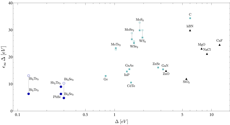
Supplementary Figure 2: Comparative figure demonstrating the conventional way of analyzing the dielectric constant as a function of the gap. Here we plot $\epsilon_{\infty}\Delta$, rather than $\left<\bar{g}\right>_{z}\propto a_{z}\Delta\chi$ (Fig. 4 of the main text). Note that there is a substantially wider spread of the datapoints between large-gap insulators and small-gap semiconductors, with $\epsilon_{\infty}\Delta$ varying by a factor of $10$ between largest to smallest values. In Fig. 4 of the main text, the dynamic range of $\left<\bar{g}\right>_{z}$ is below $2.5$.