Mapping and Probing Froggatt-Nielsen Solutions to the Quark Flavor Puzzle

Abstract

The Froggatt-Nielsen (FN) mechanism is an elegant solution to the flavor problem. In its minimal application to the quark sector, the different quark types and generations have different charges under a $U(1)_{X}$ flavor symmetry. The SM Yukawa couplings are generated below the flavor breaking scale with hierarchies dictated by the quark charge assignments. Only a handful of charge assignments are generally considered in the literature. We analyze the complete space of possible charge assignments with $|X_{q_{i}}|\leq 4$ and perform both a set of Bayesian-inspired numerical scans and an analytical spurion analysis to identify those charge assignments that reliably generate SM-like quark mass and mixing hierarchies. The resulting set of top-20 flavor charge assignments significantly enlarges the viable space of FN models but is still compact enough to enable focused phenomenological study. We demonstrate that these distinct charge assignments result in the generation of flavor-violating four-quark operators characterized by significantly varied strengths, potentially differing substantially from the possibilities previously explored in the literature. Future precision measurement of quark flavor violating observables may therefore enable us to distinguish among otherwise equally plausible FN charges, thus shedding light on the UV structure of the flavor sector.

I Introduction

The possible origin of the wide and varying hierarchies amongst the quark and lepton masses and mixing angles has long invited speculation. While such disparate Lagrangian parameters are technically natural for fermions, the fact that the three matter generations appear identical in all other respects calls for a dynamical explanation of this so-called flavor puzzle.

A common strategy is to describe these patterns in terms of an approximate flavor symmetry, a subgroup of $U(3)^{5}$, whose breaking yields the observed masses and mixing angles. Historically, the first attempt in this direction was made by Froggatt and Nielsen in 1978 [1]. This strategy, expanded in [2, 3], became known as the Froggatt-Nielsen (FN) mechanism (see e.g. Ref. [4] for a modern review). In its simplest form, this mechanism relies on the introduction of a $U(1)_{X}$ symmetry under which fermions of different generations have different charges. This symmetry is broken at some high “flavor scale” $\Lambda_{F}$ by the vacuum expectation value (vev) of a SM-singlet scalar $\phi$, often referred to as the flavon. The SM Yukawa couplings are then generated as effective operators suppressed by factors $(\langle\phi\rangle/\Lambda_{F})^{n}=\epsilon^{n}$, where $\epsilon\lesssim 0.1$ and $n$ is determined by the $U(1)_{X}$ charges of the Higgs and the respective fermions. Assuming that these operators are generated in the UV completion of the model through heavy particle exchange with presumably $\mathcal{O}(1)$ coefficients (see e.g. Refs. [5, 6, 7]), the hierarchies of the Yukawa couplings in the flavor basis are generated by the $U(1)_{X}$ charge assignments of the SM fields and the flavon vev relative to the UV scale, $\epsilon$.

FN models have been extremely well studied over the last decades (see e.g. Refs. [3, 2, 8, 9, 10, 11, 12, 5, 13, 14, 15, 16, 6, 17, 18, 7, 19, 20, 4]), but curiously, the vast literature only considered very few choices of the flavor symmetry charge assignments for the SM fields. The studied scenarios typically identify $\epsilon$ with the Cabibbo angle of the Cabibbo-Kobayashi-Maskawa (CKM) matrix and perform a spurion analysis to find a solution for the required fermion charges. The selection of these charges carries important phenomenological implications, since FN models have a variety of experimental signatures at low energies – most obviously various flavor-changing processes – the details of which depend on the exact charge assignment chosen.

In FN models of the quark sector typically discussed in the literature, flavor-changing neutral current (FCNC) constraints involving the light generations bound the flavor scale to be above $\Lambda_{F}\gtrsim 10-100$ PeV [4]. This makes FN models (like most solutions to the flavor puzzle relying on a single flavor scale $\Lambda_{F}$) notoriously hard to probe experimentally. However, the next decades may see significant advances in our ability to probe flavor violation beyond the SM, whether with new data from on-going experiments (most notably LHCb and Belle II), concrete proposals for future high-energy colliders [21, 22, 23, 24, 25, 26, 27, 28], the hypothetical possibility of future flavor factories, or theoretical advances to improve the precision of SM predictions for experimentally well-measured processes. It is thus pertinent to investigate whether experimental insights can be gained regarding FN models in the foreseeable future, despite their characteristic high energy scale.

In this paper, we perform the first step in such a model-exhaustive program by identifying the most general “theory space” of natural FN models with a single Higgs field that can address the SM flavor problem. As pointed out in Ref. [20], flavor charge assignments beyond the few canonical choices can generate close matches to the SM, seemingly with natural $\mathcal{O}(1)$ choices for the various coefficients. Inspired by this observation, our analysis considers all possible flavor charge assignments up to $|X_{q}|\leq 4$ in a FN setup restricted to the quark sector, then performs numerical scans over natural $\mathcal{O}(1)$ choices of all the Yukawa coefficients, to determine in a maximally agnostic and general fashion which charge assignments and flavon vevs can generate “SM-like” quark masses and mixings. We find that the space of fully natural FN models is much larger than previously understood in the literature, including at least several dozen models depending on the precise interpretation of our results.

Unlike previous such analyses, we select the “SM-like” choices in a Bayesian-inspired fashion without explicitly fitting to the SM. We believe this more accurately reflects the intended spirit of the FN solution, that the SM hierarchies should emerge “naturally.” Reassuringly, we do find that the SM-like FN setups easily yield many stable exact fits to the SM, and that our numerical results can be understood in the context of an analytical spurion analysis that assumes small rotations between the flavor- and mass-bases.

With this natural theory space of viable FN models now defined, we then perform a toy-demonstration of their phenomenological significance by estimating the size of various flavor-violating dimension-6 SMEFT operators in each model and comparing their size to current constraints. This not only demonstrates that distinct charge assignments or “textures” (these terms are used interchangeably hereafter) yield varying predictions for flavor-violating observables, but it also provides insights into the specific observables that are most effective in discerning between different FN solutions to the flavor puzzle in the future. It is our hope that this kind of analysis can be helpful for future studies of flavor physics, including SMEFT global fits, by providing a “theoretical lamp post” that can direct attention on the most well-motivated parts of the vast landscape of FN models and flavor observables.

This paper is structured as follows. In Section II we briefly review the Froggatt-Nielsen mechanism. The numerical analysis of all possible FN models with $|X_{q}|\leq 4$ is presented in Section III. The results of this analysis are corroborated by an analytical spurion analysis in Section IV. Some phenomenological implications are sketched out in Section V, and we conclude in Section VI. Details on SM fits, a custom tuning measure appropriate for FN models, and a variety of necessary statistical checks are collected in the Appendices.

II Review of the Froggatt-Nielsen mechanism

In this Section we briefly review the Froggatt-Nielsen mechanism in its minimal form. Our treatment and notation parallels closely that of Ref. [20]. As stated in the introduction, the FN mechanism consists of adding a new $U(1)_{X}$ global flavor symmetry to the SM, along with a scalar field $\phi$ whose vev spontaneously breaks this symmetry. Without loss of generality we take $X_{\phi}=1,X_{H}=0$ and the vev of $\phi$ to be in the positive real direction, $\braket{\phi}=\braket{\phi}^{\dagger}=\epsilon\Lambda_{F}$, where $\Lambda_{F}$ is the characteristic scale of spontaneous symmetry breaking. SM matter fields are then assigned $U(1)_{X}$ charges, forcing the scalar to appear in the SM Yukawa couplings in order to preserve the symmetry. We denote the left-handed quark doublets as $Q_{i}$ and the right-handed up- and down-quark singlets $u_{i}$ and $d_{i}$, where $i=1,2,3$ is an index running over the fermion families. The quark mass terms in the low-energy SM effective field theory then take the form:

$$\mathcal{L}_{\mathrm{Y}} \supset-c_{ij}^{u}\bar{Q}_{i}\widetilde{H}u_{j}\epsilon^{|X_{Q_{i}}-X_{u_{j}}|}-c_{ij}^{d}\bar{Q}_{i}Hd_{j}\epsilon^{|X_{Q_{i}}-X_{d_{j}}|}+\mathrm{h.c.}$$ (1)

where $H$ is the SM Higgs doublet, and $c^{u,d}$ are arbitrary $3\times 3$ complex matrices with (presumably) $\mathcal{O}(1)$ entries. Comparing Eq. 1 to the usual SM Yukawa Lagrangian

$$\mathcal{L}_{\mathrm{SM}}\supset-Y_{ij}^{u}\bar{Q}_{i}\widetilde{H}u_{j}-Y_{ij}^{d}\bar{Q}_{i}Hd_{j}+\mathrm{h.c.}\,,$$ (2)

we can read off the Yukawa matrices in terms of the FN parameters:

$$Y^{u}_{ij}=c^{u}_{ij}\epsilon^{n^{u}_{ij}}\,, Y^{d}_{ij}=c^{d}_{ij}\epsilon^{n^{d}_{ij}}\,,$$ (3)

where

$$n^{u}_{ij}=|X_{Q_{i}}-X_{u_{j}}|\,, n^{d}_{ij}=|X_{Q_{i}}-X_{d_{j}}|\,.$$ (4)

From this expression it is clear that, if $\epsilon\ll 1$, the SM Yukawa couplings can exhibit large hierarchies even if all entries of the coefficient matrices $c^{u,d}$ are $\mathcal{O}(1)$. These can be related to observable quantities – the quark masses and mixing angles – by performing unitary flavor rotations of the quark fields. Upon performing such rotations, the Yukawa Lagrangian can be written in the mass eigenstate basis, or in the so-called “up-basis”:

$$\mathcal{L}_{\mathrm{SM}}\supset-\hat{Y}_{ij}^{u}\bar{Q}_{i}\widetilde{H}u_{j}+(V_{\mathrm{CKM}}\hat{Y}^{d})_{ij}\bar{Q}_{i}Hd_{j}+\mathrm{h.c.}\ ,$$ (5)

(analogously for the “down-basis”) where $V_{\mathrm{CKM}}$ is the CKM matrix and $\hat{Y}^{u/d}$ are real, diagonal matrices, whose eigenvalues are related to the quark masses via $y_{q}\equiv\sqrt{2}m_{q}/v_{H}$, with $m_{q}$ and $v_{H}$ being the mass of the quark $q$ and the Higgs vev, respectively.

III Systematic exploration of Froggatt-Nielsen Models

We consider all possible charge assignments with $|X|\leq 4$ for all SM quarks. Since $y_{t}\approx 1$, baryon number is conserved, and permutations of the quark fields do not constitute a physical difference between FN models, we can set $X_{q_{3}}=X_{u_{3}}=0$ and adopt the ordering convention that $|X_{Q_{i}}|\geq|X_{Q_{j}}|$ for $i<j$ when all $X_{Q}$ have the same sign, otherwise $X_{Q_{i}}\geq X_{Q_{j}}$. (Similarly for $X_{u}$, or $X_{d}$.) In addition, following [20] we remove “mirror” charges which are related by multiplying all of the charges $X$ by $-1$ (and then enforcing the above ordering convention). This gives a total of 167,125 charge assignments that are physically inequivalent in the IR.

We now wish to assess these textures based on how “typical” it is for them to reproduce the flavor hierarchies of the SM. Given a certain charge assignment $\bm{X}=\left\{X_{Q},X_{u},X_{d}\right\}$, we randomly draw some large number of $\mathcal{O}(1)$ complex coefficient matrices $c^{u,d}$ (details discussed below) and calculate the SM parameters for each instance of $c^{u,d}$ as a function of $\epsilon$. For a given choice of $\epsilon$, we can then calculate the observable with the maximum fractional deviation from its SM value:

$$\Xi_{\mathrm{SM}}=\max_{i}\exp\Bigg{|}\ln\left(\frac{\mu_{i}^{\text{guess}}}{\mu_{i}^{\text{SM}}}\right)\Bigg{|}\ ,$$ (6)

where $\mu_{i}$ ranges over the six quark masses, the three independent CKM entries $|V_{12}|,|V_{13}|$, and $|V_{23}|$, and the absolute value of the Jarlskog invariant $|J|$. The precise numerical values we use can be found in Table 2 in Appendix B. Since $\epsilon$ plays the central role of generating the overall hierarchy, we minimize $\Xi_{\mathrm{SM}}$ with respect to $\epsilon$ for each instance of the $c^{u,d}$ coefficient matrices to match as closely as possible the SM values.

Num.	$X_{Q_{1}}$	$X_{Q_{2}}$	$X_{u_{1}}$	$X_{u_{2}}$	$X_{d_{1}}$	$X_{d_{2}}$	$X_{d_{3}}$	$\mathcal{F}_{2}\;(\%)$	$\mathcal{F}_{5}\;(\%)$	$\epsilon$
1	3	2	-4	-2	-3	-3	-3	2.7	67	0.17
2	3	2	-4	-2	-4	-3	-3	2.5	66	0.18
3	3	2	-3	-1	-3	-2	-2	1.9	56	0.12
4	3	2	-4	-1	-3	-3	-3	1.5	65	0.16
5	4	3	-4	-2	-4	-3	-3	1.2	52	0.23
6	3	2	-4	-1	-3	-3	-2	1.1	63	0.15
7	4	2	-4	-2	-4	-3	-3	1.1	47	0.21
8	3	2	-3	-1	-2	-2	-2	0.9	41	0.11
9	3	2	-3	-1	-3	-3	-2	0.9	55	0.14
10	3	2	-4	-2	-3	-3	-2	0.9	59	0.16
11	2	1	-3	-1	-2	-2	-2	0.8	52	0.06
12	4	3	-4	-1	-4	-3	-3	0.8	52	0.22
13	4	3	-4	-2	-4	-4	-3	0.8	50	0.24
14	3	2	-4	-2	-4	-3	-2	0.7	56	0.17
15	4	3	-4	-2	-3	-3	-3	0.7	43	0.22
16	4	3	-4	-1	-3	-3	-3	0.6	45	0.21
17	4	2	-4	-2	-4	-4	-3	0.6	48	0.22
18	4	2	-4	-2	-3	-3	-3	0.6	38	0.2
19	3	2	-4	-1	-3	-2	-2	0.6	56	0.14
20	3	2	-3	-2	-3	-3	-2	0.6	45	0.15

Table 1: The top 20 textures ranked by the fraction of the time that a random draw of $c^{u,d}$ coefficient matrices result in all quark masses, CKM matrix elements, and the Jarlskog invariant within a factor of $2$ of the SM (allowing $\epsilon$ to vary to minimize deviation from the SM). For each texture, $\mathcal{F}_{2}$ ($\mathcal{F}_{5})$ is the fraction within $2$ (5), and $\epsilon$ is the average value of $\epsilon$ for those coefficients that end up within a factor of $2$. For all of these textures, $X_{Q_{3}}=X_{u_{3}}=0$.

After repeating this process for each charge assignment $\bm{X}$, we define $\mathcal{F}_{2}$ ($\mathcal{F}_{5}$) as the fraction of random coefficient choices that yields $\Xi_{\mathrm{SM}}\leq 2$ $(5)$ for each model. This allows us to define “global naturalness criteria” (i.e. independent of a particular fit to the SM) for a given texture to be a good candidate for reproducing the SM hierarchies, namely requiring that $\mathcal{F}_{2}$ or $\mathcal{F}_{5}$ be above some lower bound.

Out of the total 167,125 possible charge assignments, we only find about 10 for which $\mathcal{F}_{2}\gtrsim 1\%$. We adopt the latter criterion as the most stringent measure of naturalness for a texture to solve the SM quark flavor problem, and show the top-20 possible charge assignemnts ranked by $\mathcal{F}_{2}$ in Table 1.We also show the average value of $\epsilon$ for each texture. The distribution of preferred $\epsilon$ values is very narrow, indicating that each texture has a uniquely suited value of $\langle\phi\rangle/\Lambda_{F}$ to reproduce the SM. Some of these good textures correspond to those identified already in the literature, but, to the best of our knowledge, most of them have not been considered before.

This is quite remarkable, given how similarly they all naturally generate SM-like mass and mixing hierarchies. Textures where all quark masses and CKM entries lie within a factor of 5 of their measured SM values are even more common, with about 430 textures satisfying $\mathcal{F}_{5}\gtrsim 10\%$. This constitutes a large collection of textures that are well-motivated in this model-independent way. The complete ranking of these textures is included in the file charges.csv provided in the auxiliary material.

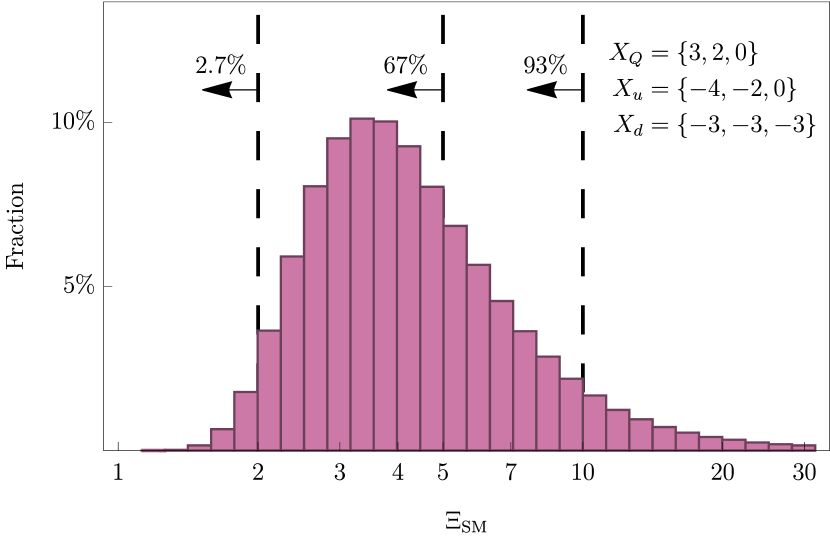
Figure 1: A probability distribution function for $\Xi_{\mathrm{SM}}$ for the top-ranked texture in Tab. 1. To produce this plot we randomly generate many different choices of $c^{u/d}$ matrices and compute $\Xi_{\mathrm{SM}}$ for each one (allowing $\epsilon$ to vary to minimize deviation from the SM). Also shown are the total fraction of coefficient matrices that result in $\Xi_{\mathrm{SM}}<2,5,\text{and }10$ respectively. For this texture, typical random $\mathcal{O}(1)$ matrices of coefficients will result in all quark masses and CKM parameters within a factor of $\approx 4$ of their measured SM values.

As mentioned above, to understand how close a texture generically is to the SM, we may look at the distribution of $\Xi_{\mathrm{SM}}$ values for a given texture over many different random choices of the $c^{u,d}$ matrices. In Fig. 1, we show such a distribution for the top texture from Table 1. As we can see, the distribution is clustered around $\Xi_{\mathrm{SM}}\sim 4$ with broad tails on either side, indicating that this texture generically results in physical parameters with the proper SM-like hierarchies regardless of the $\mathcal{O}(1)$ coefficients $c^{u,d}$. Of course getting the precise SM values requires a precise choice of these coefficients, but the hierarchies themselves are robust.

We may also look at such a distribution for a charge assignment that does not perform well by this metric. This category includes many textures previously mentioned in the literature, including for example most of the textures listed in Tables 1 and 2 of Ref. [20]. The third texture in Table 2 of [20] results in the distribution for $\Xi_{\mathrm{SM}}$ shown in Fig. 2. It is quite reasonable to ask why these textures show up as good in that analysis but not ours, and the answer is simple: Ref. [20] searches for textures for which there is at least one technically natural choice of $c^{u,d}$ coefficients that approximately reproduces the SM, whereas we look for textures which generically produce SM-like hierarchies. With random $\mathcal{O}(1)$ coefficient matrices, a texture like that of Fig. 2 results in a typical deviation from SM parameters of more than an order of magnitude, but there does exist a very special choice of $c^{u,d}\sim\mathcal{O}(1)$ that results in the SM. This choice of coefficients may be technically natural but it is still exceedingly rare, as Fig. 2 shows. The difference thus stems from our “global” choice of metric for naturalness, which prioritizes textures that can lead to SM-like parameters without need for additional dynamics or precise restrictions on the coefficients.

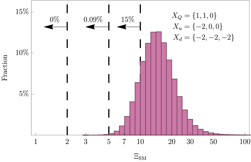
Figure 2: Similar to Fig. 1 for a texture that does not perform well by our metric. This texture does have a technically natural fit to the SM (as found in Ref. [20]), but typical $\mathcal{O}(1)$ coefficient matrices for this texture result in deviations of more than an order of magnitude from the measured SM parameters.

To verify that our global naturalness criterion also produces viable and “locally natural” solutions to the SM flavor problem, we also have to check that each of the textures in Table 1 yields exact and untuned numerical fits to the SM, including uncertainty on the SM parameters. This necessitates the definition of a custom tuning measure that is more appropriate for FN models than standard choices like the Barbieri-Giudice measure [34, 35], taking into account that any change in the UV theory would likely perturb all coefficients in Eq. 1 at once, rather than one at a time. The details are in Appendix A, but the upshot is that each of the textures in Table 1 readily yields many good SM fits that are completely untuned with respect to simultaneous random uncorrelated perturbations of all coupling coefficients. This confirms that our global naturalness criterion guarantees particular technically natural solutions to the SM flavor problem as well.

We perform several statistical checks to make sure our conclusions are robust. The results obtained here depend on the details of the statistical distributions from which we draw the coefficients in the $c^{u,d}$ matrices. Taking a Bayesian-inspired point of view, these distributions can be thought of as prior probability distributions for the $c^{u,d}$ coefficients. For the analysis shown here, we use a “log-normal” prior in which the logarithm of the magnitude of each $c^{u,d}$ entry is drawn from a Gaussian distribution. We have repeated the same analysis for a wider log-normal distribution, and a third “uniform” prior, in which the real and imaginary parts of each $c^{u,d}$ are drawn uniformly from the range $[-3,3]$. Up to modest reorderings in our ranked list of top textures, our results are robust with respect to changing the prior. We also confirm that the SM-like hierarchies for our good textures are robustly determined by the flavor charges and the small $\epsilon$ rather than anomalous hierarchies amongst the randomly drawn $c^{u,d}$ coefficients, and that individual SM observables are roughly uncorrelated and drawn from a distribution roughly centered on the correct SM value for each good texture. For details, see Appendix B.

IV Analytical Spurion Analysis

Our numerical study identified many new plausible FN textures beyond those that have been studied in the literature. It would be useful to understand analytically why the textures in Table 1 reliably yield SM-like hierarchies. If viable FN models involve no large rotations between the flavor- and the mass-basis, then it is possible to estimate masses and mixings via an analytical spurion analysis. We can easily test this assumption.

In general, the flavor-basis Yukawa matrix $Y^{u}$ (identically for $Y^{d}$) can be related to the diagonal mass-basis Yukawa $\hat{Y}^{u}$ via the usual singular value decomposition $Y^{u}=U_{u}\hat{Y}^{u}W_{u}^{\dagger}$. Under the near-aligned assumption, and adopting the strict ordering of charges defined at the beginning of Section III, the mass-basis Yukawa couplings are simply given by

$$\hat{Y}^{u}_{ij}\sim\epsilon^{n^{u}_{ii}}\delta_{ij}$$ (7)

where the exponent matrices $n^{u,d}$ are defined terms of the $X_{Q,u,d}$ charges in Eq. 4. Under the same strict assumptions, the magnitudes of the elements of the rotation matrices can be written as

$$(U_{u})_{ij} \sim \left\{\begin{array}[]{lll}1&&i=j\\ \epsilon^{n^{u}_{ij}-n^{u}_{jj}}&&i<j\\ \epsilon^{n^{u}_{ji}-n^{u}_{ii}}&&i>j\end{array}\right.$$ (11)

$$(W_{u})_{ij} \sim \left\{\begin{array}[]{lll}1&&i=j\\ \epsilon^{n^{u}_{ji}-n^{u}_{jj}}&&i<j\\ \epsilon^{n^{u}_{ij}-n^{u}_{ii}}&&i>j\end{array}\right.\ .$$ (16)

This makes it straightforward to obtain magnitude estimates for the elements of $V_{\mathrm{CKM}}=U_{u}^{\dagger}U_{d}$.

For a given FN charge assignment and choice of $\epsilon$, we can now compute the spurion estimate $\mu_{i}^{\text{spurion}}$ for $i=$ each of the six quark masses and $|V_{\mathrm{CKM}}|_{12,23,13}$. To assess how SM-like a given FN charge assignment is, we consider the logs of the ratios by which these estimates deviate from the SM, added in quadrature,

$$d=\left[\sum_{i}\log_{10}^{2}\left(\frac{\mu_{i}^{\text{spurion}}}{\mu_{i}^{\text{SM}}}\right)\right]^{1/2}\ ,$$ (17)

with $\epsilon$ chosen to minimize $d$. This measure always takes all SM observables into account and is more appropriate for the approximate nature of the spurion analysis than Eq. 6. We would expect that FN textures that naturally give a good fit to the SM would satisfy $d\lesssim\mathcal{O}(1)$.

Indeed, we find that all the textures in Table 1 satisfy $d<2.4$. Of all 167,125 possible charge assignments, there are only 36 additional possibilities that also satisfy this criterion, and all of them are in the top 160 of our ranked list of textures obtained in the numerical analysis of the previous section. This analytical spurion estimate is therefore fully consistent with our full numerical study, which gives us additional confidence that the global naturalness criterion derived in our numerical study is theoretically plausible. Furthermore, this convergent result confirms the expectation that natural FN models always feature a high degree of alignment between the flavor and the mass bases.

Obviously, the specific $d<2.4$ criterion was derived a posteriori from the results of the numerical study, but if one were to guess at a reasonable upper bound for $d$ that natural SM-like FN models must satisfy, a number like $d<3$ might plausibly come to mind, which yields a still very modest total of 149 textures (including the top 20). As with any such definition, the cutoff for what constitutes a natural model is somewhat arbitrary, and if one wants to make quantitative statements the fully numerical approach of the previous section is necessary. However, it is interesting to note that the numerical study was not necessary to make the much more important qualitative observation that there are many different FN charge assignments, of the order of several dozen at least, that very naturally give SM-like hierarchies. The crucial ingredient is merely to formulate a well-defined and general criterion and check it across all possible flavor charges.

V Phenomenological Implications

Flavor-violating effects are the most relevant experimental signatures of FN models. At low energies these can be effectively parameterized within the framework of Standard Model Effective Field Theory (SMEFT). Our focus here lies on examining 4-fermion operators of the form

$$\mathcal{O}=\frac{1}{\Lambda_{\mathrm{eff}}^{2}}(\bar{q}_{i}q_{j})(\bar{q}_{k}q_{l})$$ (18)

where $i,j,k,l$ denote different quark flavors, and $q$ can represent either $Q,d$ or $u$ type quarks. While semi-leptonic and fully leptonic 4-fermion operators can also be generated, 4-quark operators are most important for our discussion, given that we assign FN charges only to the quarks. (For the sake of simplicity, Dirac structures as well as Lorentz and group indices are left implicit.)

We can estimate the size of these operators using a spurion analysis analogous to the estimates for SM quantities in the last section. In the “FN flavor basis” of Eq. 3, where flavor charges are well-defined for each quark generation, the leading contribution to the coefficient of this operator will take the form

$$\frac{1}{\Lambda_{\mathrm{eff}}^{2}}=c_{\mathcal{O}}\frac{\epsilon^{|-X_{q_{i}}+X_{q_{j}}-X_{q_{k}}+X_{q_{l}}|}}{\Lambda_{F}^{2}}\ .$$ (19)

where $\Lambda_{F}$ is the UV scale of the model (with $\epsilon=\langle\phi\rangle/\Lambda_{F}$), and $c_{\mathcal{O}}$ is an unknown dimensionless complex coefficient. For FN models that satisfy our global naturalness criterion, it is plausible to expect the different coefficients $c_{\mathcal{O}}$ to be relatively uncorrelated and have modest $\mathcal{O}(1)$ sizes.

The ‘SM-like’ FN textures we find and list in Table 1 are equivalently suitable for generating the SM quark Yukawa coupling matrices. However, they predict quite disparate flavor-violating signatures, and future measurements hold the potential to not only detect these non-standard flavor violating-effects but also distinguish between possible natural flavor textures. Such investigations could provide valuable insights into unraveling the true structure of the flavor sector.

To demonstrate these parametric differences quantitatively, we work in the Warsaw basis [37] and obtain bounds on the 4-quark-operator Wilson coefficients using the global likelihood implemented in the Python package smelli [38, 39, 40]. For simplicity, we only turn on one operator at a time (since we merely want to demonstrate the significant differences between different FN charge assignments), and take the bound on $\Lambda_{\mathrm{eff}}$ for each operator to correspond to the most constraining bound obtained by turning the operator on with purely real or imaginary positive or negative coefficient. Since $c_{\mathcal{O}}$ is likely to have a “random phase” in the FN model, this is the most conservative assumption for our demonstration.

Some care must be taken to obtain physically consistent results from this spurion estimate for 4-quark operators. smelli supplies bounds in the down-aligned (or up-aligned) interaction basis, where the right-handed $u,d$ fields are rotated using the $W_{u,d}$ matrices estimated in Eq. LABEL:e.UW, while $Q$ is rotated using $U_{d}$ ($U_{u}$). As a result, $u_{R},d_{R}$ and $d_{L}$ ($u_{L}$) are mass eigenstates, while the $u_{L}$ ($d_{L}$) fields are rotated by $V_{\mathrm{CKM}}$ with respect to their mass eigenstate basis. This obviously results in bounds on operator coefficients being different in the up- and down-aligned basis, simply because the make-up of each 4-Fermi operator in terms of quark-mass-basis operators is different. In an exact numerical analysis of FN models — where for a given FN charge assignment one might choose random $c_{ij}^{u,d}$ restricted to give good fits to SM masses and mixings; then consider random numerical trial values for the $c_{\mathcal{O}}$’s in the FN flavor basis; and finally perform exact rotations into the up- or down-aligned basis — the resulting bounds on $c_{\mathcal{O}}/\Lambda_{F}^{2}$ in the FN flavor basis would be exactly equivalent in the two bases. However, in our parametric spurion estimates, while it seems one could use the transformation matrix estimates of Eq. LABEL:e.UW to obtain 4-Fermi operator estimates in the up- or down-aligned bases, in reality this fails to reliably capture differences between the operator definitions at sub-leading order in $\epsilon$. Differences between the two bases enter exactly at this order, but this still results in large differences in the numerical bounds on operator coefficients, since in some cases the leading bound on an up- or down-basis operator comes from a mass-basis contribution to that operator that is sub-leading in CKM mixing angles, but can nonetheless supply the dominant bound due to the severity of the corresponding physical constraint.

Fortunately, the important effects that are CKM-suppressed in the up-aligned basis are leading-order in the down-aligned basis, and vice versa. Furthermore, the close alignment between the FN flavor basis, up-aligned basis, down-aligned basis and mass-basis (evident from the near-diagonal nature of the $U_{u,d},W_{u,d}$ in Eq. LABEL:e.UW) means that the FN flavor basis predictions of Eq.19 apply, to leading order in $\epsilon$, in the up- and down-aligned bases as well. Taking these two observations together, we find that we can obtain physically consistent parametric estimates of the bounds on $c_{\mathcal{O}}/\Lambda_{F}^{2}$ in the FN flavor basis by comparing the predictions of Eq.19 to the constraints supplied by smelli in both the up- and down-aligned basis, and simply adopting the stronger of the two bounds for that operator.

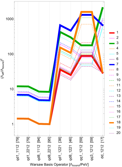
Figure 3: Relative size of a demonstrative sub-set of flavor-violating 4-quark operators in the Warsaw operator basis and FN flavor quark basis for each of the 20 “most natural” FN models in Table 1, for a flavor scale of $\Lambda_{F}=100$ PeV, compared to their current bound assuming $c_{\mathcal{O}}=1$. Models 1, 3, 7 and 18 are emphasized to demonstrate the qualitatively different configurations of flavor-violating operators that can be generated by natural FN models. The number in brackets after the operator label on the horizontal axis is the lower bound on $\Lambda_{\mathrm{eff}}$ in PeV.

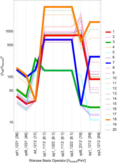
Figure 4: Same as Figure 3, but for each texture the flavor scale $\Lambda_{F}$ is separately chosen to saturate its current bounds. The operators qd(1,8)_(2212,1112) that dominate the $\Lambda_{F}$ bound and have similar predictions for all considered textures are omitted, and instead some additional operators are shown.

We find that all textures in Table 1 are constrained to have a flavor scale $\Lambda_{F}\gtrsim$ 40 - 100 PeV. Setting $\Lambda_{F}=100$ PeV for all textures, we show in Fig. 3 the relative size of some operators compared to their current bound, for a subset of operators with predicted size not too far from current constraints. The operators which dominate the bound on $\Lambda_{\mathrm{F}}$ are qd8_2212, qd8_1112, qd1_2212, qd1_1112, which also show the least variation between textures. However, there is a large degree of variation amongst the other operators with predictions that are a factor of $\gtrsim 10$ beyond current bounds. Four textures have been highlighted to showcase this variation in the prediction of various flavor-violating quark operators: the top texture #1 in red, the “original” FN texture [3, 2] #3 in green, and two others, #7 and #18, in blue and orange. Note that each prediction has a “theoretical uncertainty” of $\mathcal{O}(1)$ in this plot, due to the unknown size of the $c_{\mathcal{O}}$ coefficients.

To further emphasize the differences in the relative predictions for flavor-violating quark operators, rather than different overall suppression of flavor-violating effects, Figure 4 shows the predictions for a subset of operators where the flavor scale has been set to its current bound separately for each texture. We do not show the four operators qd(1,8)_(2212,1112), which dominate the $\Lambda_{F}$ bound and have similar predictions for all considered textures, but we now show some additional operators that display large variation between textures under these new assumptions. This explicitly demonstrates that if a given non-SM flavor-violating effect were found (setting the absolute size of some flavor-violating operators), the resulting predictions for the other flavor-violating operators would differ widely amongst equally natural FN models.

Unsurprisingly, the observables that drive the bound on these most “distinguishing” coefficients are those related to quark flavor mixing in the 1-2 sector, in particular to the imaginary part of the $D-\bar{D}$ and $K-\bar{K}$ mixing amplitudes, encoded in $x_{12}\sin\phi_{12}$ and $\epsilon_{K}$, respectively. For kaon mixing, the current bottleneck preventing tighter constraints is the uncertainty in the SM prediction for $\epsilon_{K}$. Future improvements may be possible, but are hard to predict. On the other hand, a significant improvement is expected in the experimental determination of the parameters describing CP violation in $D-\bar{D}$ oscillations. In particular, the uncertainty on the imaginary part of the amplitude is expected to shrink at least of a factor $5$ at the end of Upgrade II of the LHCb experiment [44]. There has also been significant recent work on global SMEFT fits under certain flavor violating hypotheses (see e.g. [45, 46, 47, 48]). Our menu of natural FN models is a natural candidate for future analyses of this kind, which may yet yield unexpected constraints on particular models considered in a global fit.

VI Conclusions

The flavor puzzle is a vexing mystery of the Standard Model, with the pattern of the fermion mass matrices hinting at the presence of a deeper structure. Directly probing the mechanisms that generate this structure is difficult, as tight constraints on flavor violation usually push the relevant scale of flavor physics to very high values far beyond our ability to probe directly in the intermediate future. Even so, the advent of future experiments makes direct or indirect detection and diagnosis of this underlying flavor structure an enticing prospect.

Our work provides a theoretical roadmap to help navigate the potentially vast space of Froggatt-Nielsen solutions to the quark flavor problem. It dramatically enlarges the space of viable charge assignments compared to what has been studied in the literature, but our global criterion of naturally generating the SM mass and mixing hierarchies across the model’s whole parameter space is still constraining enough to net a manageable number of FN models, see Table 1.

We showed that this well-defined subset of FN benchmark models generates a variety of different flavor-violating operators within the SMEFT framework, with widely varying magnitudes depending on the flavor charge assignments. In principle this makes diagnosing the solution to the quark flavor problem plausible once flavor-violating signals beyond the SM expectation are unambiguously observed. Global SMEFT fits that assume a particular FN model can be even more constraining [45, 46, 47, 48], and it would be interesting to conduct such fits for each of the natural FN models we identify in Table 1 for well-defined priors on the unknown $\mathcal{O}(1)$ coefficients of the model.

Our method of finding natural FN models naturally generalizes to FN models of the lepton sector, or non-minimal setups with multiple or non-abelian flavor symmetries [49, 50, 51, 52, 53]. This may suggest further flavor-violating observables that have the most promise of detecting and diagnosing the physics of the flavor puzzle. It may also be interesting to study the impact of our work on dark sectors that are related to the SM via a discrete symmetry [54]. We leave such investigations for future work.

Appendix A Standard Model Fits and Tuning

SM parameter	Value
$m_{u}$	0.00117(35)
$m_{c}$	0.543(72)
$m_{t}$	148.1(1.3)
$m_{d}$	0.0024(42)
$m_{s}$	0.049(15)
$m_{b}$	2.41(14)
$|V_{12}|$	0.22450(67)
$|V_{13}|$	0.00382(11)
$|V_{23}|$	0.04100(85)
$|J|$	3.08(14) $\times 10^{-5}$

Table 2: Standard Model parameters and uncertainties used to compute goodness-of-fit parameters such as $\Xi_{\mathrm{SM}}$ (Eq. 6) Quark masses (given in GeV) are taken from [55], evaluated at $\mu=1$ TeV. Running these parameters to the $\mathcal{O}$(PeV) flavor scale would not significantly change our results. CKM parameters are taken from the PDG review [41], evaluated at low scales; we explicitly checked that including the running of the CKM parameters does not have any noticeable effect on our analysis.

In this appendix we present details on finding solutions for the coefficients $c_{ij}^{u,d}$ in Eq. 3 that represent realistic SM fits within experimental uncertainties for the quark masses and mixings, see Table 2, for each of the FN charge assignments in Table 1.

In order to obtain SM fits, we used a simplex minimization algorithm to adjust the coefficients $c_{ij}^{u,d}$ and the parameter $\epsilon$ in order to optimize the standard $\chi^{2}$ score,

$$\chi^{2}_{\rm SM}=\sum_{i}\left(\frac{\mu_{i}-\mu_{i}^{\rm SM}}{\sigma_{i}^{\rm SM}}\right)^{2}$$ (20)

where as in Sec. III the index $i$ runs over all of the SM quark masses, three CKM mixing angles, and $|J|$. For all of the textures in Table 1, we are able to find fits with average deviation of less that 2$\sigma$ over all 10 parameters that we fit to; we were further able to find fits with average deviation less than 1$\sigma$ for more than half of the textures in the table, including all of the top 5. We have further verified that for these fits, the values of the coefficients $c_{ij}^{u,d}$ do not have a significantly different distribution than the prior used to generate the same coefficients for our numerical scans, indicating that the fits do not require any substantial drift away from our $\mathcal{O}(1)$ assumption. Our final check is to verify that these fits are not locally tuned.

A standard tuning test is the Barbieri-Giudice measure [34, 35], which for a single SM observable $\mathcal{O}_{K}$ can be defined as:

$$\Delta_{\mathrm{BG}}^{K}\equiv\max_{k}|\delta_{K,k}| \delta_{K,k}\equiv\frac{\delta\log\mathcal{O}_{K}}{\delta\log c_{k}}\ ,$$ , (21)

where $c_{k}$ runs separately over the real and imaginary parts of each of the $c_{ij}^{u,d}$ coefficients defined in Eq. 3. A second maximization then gives the overall tuning taking into account all fitted SM observables:

$$\Delta_{\mathrm{BG}}\equiv\max_{K}\Delta_{\mathrm{BG}}^{K}\ .$$ (22)

This basically represents the maximum sensitivity of all the 10 SM observables $\mathcal{O}_{K}$ with respect perturbing any single one of the 18 complex coefficients $c_{ij}^{u,d}$. However, we argue that for Froggatt-Nielsen models and their many coefficients, which arise from some UV theory, this tuning measure is of limited utility, since a small change in the UV theory would slightly change all the coefficients at once, not just one at a time. Indeed, if random small permutations of some characteristic size are applied to all $c_{ij}^{u,d}$ coefficients of a given SM fit, we numerically find that $\Delta_{\mathrm{BG}}^{K}$ generally significantly underestimates the variance of a given SM observable $\mathcal{O}_{K}$. In other words, for FN models, the Barbieri-Giudice measure underestimates tuning.

Some way of assessing this total sensitivity is required. We therefore define the following tuning measure for each SM observable $\mathcal{O}_{K}$:

$$\Delta_{\mathrm{tot}}^{K}\equiv\left[\sum_{s}(\lambda^{K}_{s})^{2}\right]^{1/2}$$ (23)

where the $\lambda_{s}^{K}$ are the eigenvalues of the matrix $\Delta_{kl}^{K}$ defined as

$$\Delta_{kl}^{K}\equiv\frac{\delta^{2}\log\mathcal{O}_{K}}{\delta\log c_{k}\delta\log c_{l}}$$ (24)

and $c_{k}$ runs over the real and imaginary parts of all $c_{ij}^{u,d}$ coefficients as above. It is easy to see that this quantity could give a more complete account of the tuning of a given SM fit, since the sum in quadrature over the principal directions of $\Delta_{kl}^{K}$ takes into account the total variability of SM observable $\mathcal{O}_{K}$, regardless of whether the direction of maximum sensitivity is aligned with any one $c_{ij}^{u,d}$, which is appropriate when perturbing all coefficients at once. Indeed, when varying all coefficients by random perturbations of characteristic relative scale $\sigma$, we find that $\Delta^{K}_{\mathrm{tot}}\sigma$ gives a very good direct estimate of the resulting relative variance of $\mathcal{O}_{K}$. This supports the argument that $\Delta_{\mathrm{tot}}^{K}$ is a more faithful measure of sensitivity to changes in the underlying UV theory of a FN model, and an overall tuning measure for the whole SM fit can be obtained by summing in quadrature over all SM observables:

$$\Delta_{\mathrm{tot}}=\left[\sum_{K}(\Delta_{\mathrm{tot}}^{K})^{2}\right]^{1/2}$$ (25)

Rank by this prior	Rank in Tab. 1	$\mathcal{F}_{2}\;(\%)$	$\mathcal{F}_{5}\;(\%)$	$\epsilon$
1	1	0.17	24	0.16
2	2	0.13	22	0.17
3	3	0.12	19	0.12
4	16	0.11	19	0.2
5	8	0.1	17	0.1
6	15	0.1	18	0.21
7	18	0.1	14	0.18
8	11	0.1	16	0.06
9	12	0.09	19	0.21
10	10	0.09	18	0.15

Table 3: Analogue of Table 1 for top-10 textures and their $\mathcal{F}_{2}$, $\mathcal{F}_{5}$, and average $\epsilon$, but using the “wider log-normal” prior for the coefficients of the $c^{u,d}$ matrices. For comparison, we also show their rank in Table 1 in the second column. The overall fraction of $c^{u,d}$ matrices with this prior that give good fits to the SM is smaller for all textures, which is to be expected because this prior allows for larger random hierarchies in the $c^{u,d}$ coefficients and thus washes out the effect of the texture itself in generating the SM hierarchies. Textures that are perform well in Tab. 1 also perform well with this prior, although the exact ordering is somewhat shuffled.

Rank by this prior	Rank in Tab. 1	$\mathcal{F}_{2}\;(\%)$	$\mathcal{F}_{5}\;(\%)$	$\epsilon$
1	1	4.0	71	0.15
2	2	3.2	79	0.16
3	[23]	0.6	40	0.14
4	13	0.4	48	0.22
5	5	0.4	46	0.21
6	4	0.4	58	0.14
7	[22]	0.4	78	0.17
8	[21]	0.3	46	0.13
9	9	0.2	62	0.14
10	[28]	0.2	39	0.24

Table 4: Analogue of Table 1 for top-10 textures and their $\mathcal{F}_{2}$, $\mathcal{F}_{5}$, and average $\epsilon$, but using the “uniform flat” prior distribution for the coefficients of the $c^{u,d}$ matrices. For comparison, we also show their rank in Table 1 in the second column. The textures with rank in [square brackets] do not appear in Table 1, but we show their rank if that table was continued to the top-30. These textures have the following charges: rank 3 (this table), {3, 2, -3, -2, -3, -3, -3}; rank 7, {3, 2, -4, -2, -4, -4, -3}; rank 8, {3, 2, -3, -2, -3, -3, -2}; rank 10, {4, 3, -4, -2, -4, -4, -4}.]

We find that it is generally easy to find SM fits for the top-20 textures in Table 1 that have $\Delta_{\mathrm{tot}}\lesssim$ a few, proving that these solutions to the SM flavor problem are truly untuned with respect to the underlying details of the UV theory. Informally, we notice that there seems to be a trend that the $\Delta_{\mathrm{tot}}$ of an average SM fit increases modestly for lower-ranked textures in Table 1. While further study would be required to solidify this relationship, it provides further suggestive evidence that our global naturalness criterion of ranking textures by their $\mathcal{F}_{2}$ or $\mathcal{F}_{5}$ fractions is the fundamental measure of how SM-like a texture wants to be, and how natural any SM fits are that do exist.

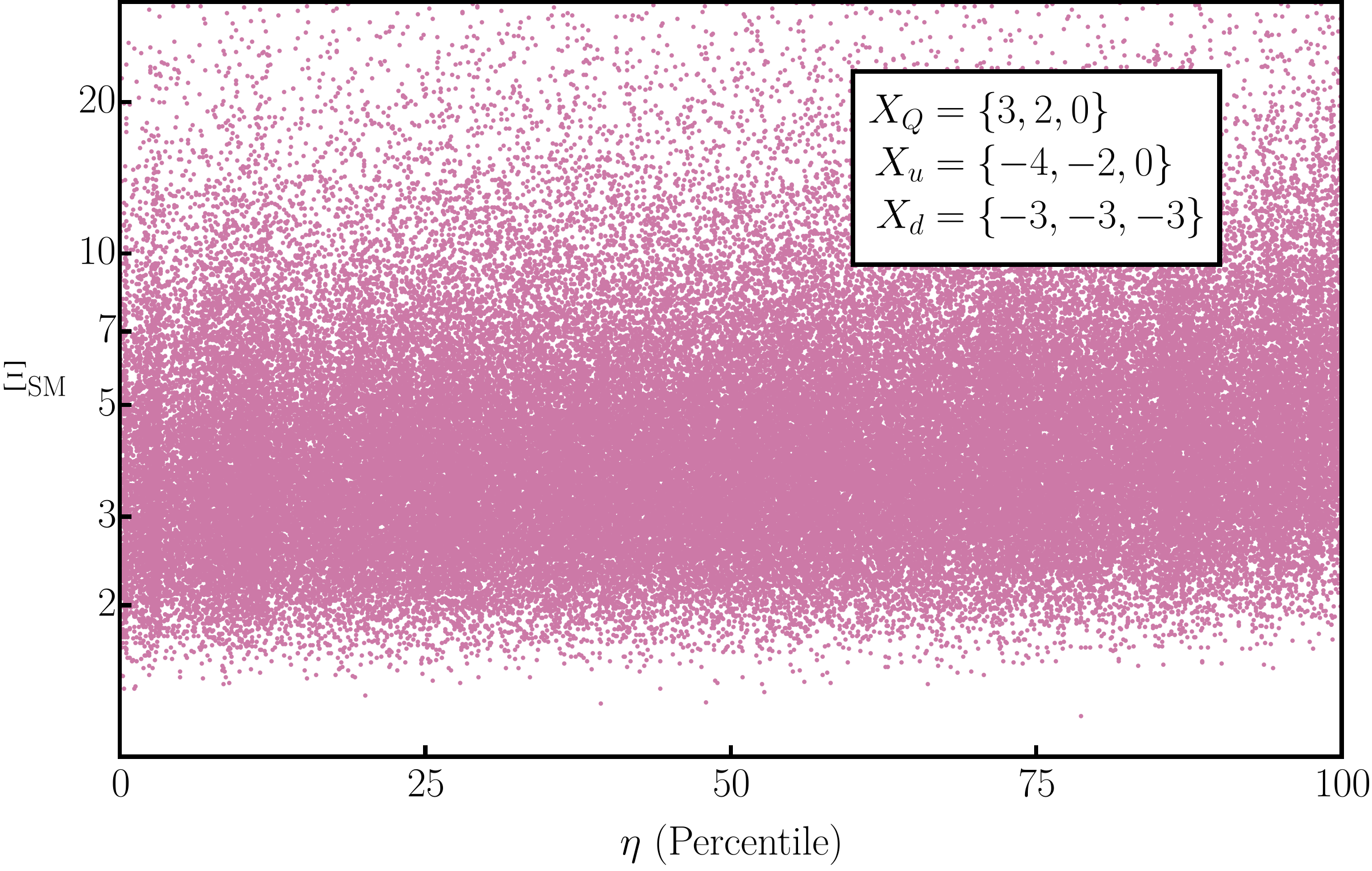
Figure 5: Correlation between closeness to the SM ($\Xi_{\mathrm{SM}}$) and how anomalous the random hierarchy between the largest and smallest $c_{ij}^{u,d}$ coefficients is (anomalous here means a particularly low or high $\eta$ pecentile), for the example of the top texture in Table 2. The lack of clear correlation demonstrates that the SM-like hierarchies do not rely on accidental hierarchies amongst the coefficients in Eq. 3.

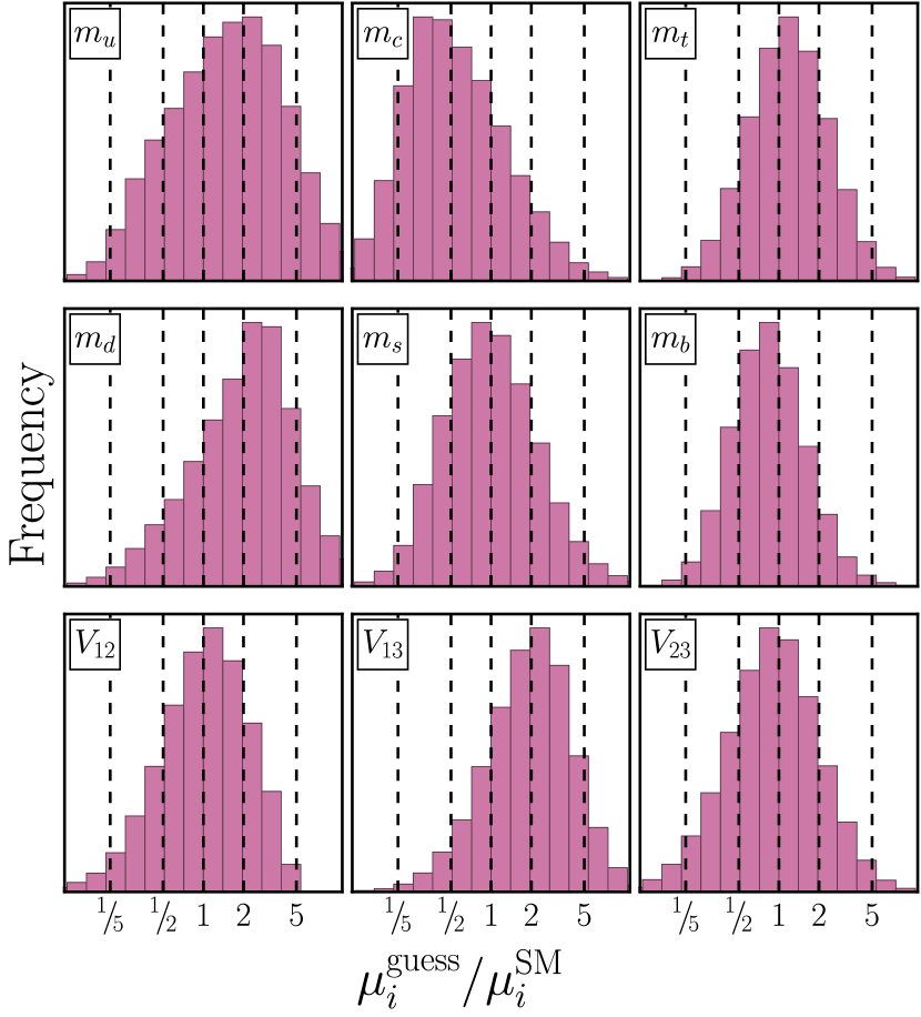
Figure 6: Individual parameter distributions for the best texture listed in Table 1. For the quark masses and the three independent CKM elements, each histogram shows the distribution of one particular parameter relative to its true SM value. For this texture, all parameter distributions are peaked within a factor of a few from their SM values. Although not shown here, there is minimal cross-correlation between any pair of these parameters.

Appendix B Dependence on prior distributions and statistical checks

In this appendix we collect the details of the prior distributions and statistical measures we use in our analysis. Because one of the main products of this paper is a collection of “statistically good” textures, i.e. a collection of textures which do a good job of reproducing SM-like hierarchies for somewhat arbitrary $\mathcal{O}(1)$ Yukawa coefficients $c^{u,d}$, it is important to understand how much these results depend on our priors for these coefficients. While we do find that the precise numbers claimed here depend on this distribution, our derived list of good textures is robust with respect to the exact choice of prior for the coefficients, up to some minor reordering.

For all results shown in the main body of this paper, our numerical scan generated the entries of $c^{u,d}$ as follows: for each coefficient independently, a magnitude was drawn from a log normal distribution centered around 1 with a standard deviation of $\ln 10^{0.3}$ (to enforce that all coefficients in the matrix be $\mathcal{O}(1)$), and a phase was drawn from a flat distribution between $0$ and $2\pi$. This choice yields the results shown in Table 1, namely that there are a few textures for which $\mathcal{O}(2\%)$ of randomly generated coefficients yield quark masses and CKM elements within a factor of 2 of their SM values, and $\mathcal{O}(50\%)$ yield parameters within a factor of 5.

In order to check that this list is robust to other choices of distribution, we ran two other scans for all charge assignments:

1. A “wider log-normal” scan where we drew the $c^{u,d}$ coefficients with a uniform distribution in phase and a log-normal distribution in magnitude centered on 0 and with a standard deviation of $\ln 10^{0.6}$.

2. A “uniform flat” scan where we drew the real and imaginary parts of each entry of $c^{u,d}$ separately from uniform flat distributions between $-3$ and $3$.

The lists of the top 10 textures (ranked by the fraction $\mathcal{F}_{2}$ within a factor of 2 of the SM value) for each of these scans are given in Tables 3 and 4. We can see that the rough list and ordering of textures in the top $5$ is not significantly changed by any of these choices, so we conclude that this data is robust to changes of distribution (provided all entries of $c^{u,d}$ be $\mathcal{O}(1)$).

Another reasonable concern that one may have about these results is whether the observed hierarchies are primarily coming from the texture choice. Our prior distribution for $c^{u,d}$ is chosen to result in $\mathcal{O}(1)$ coefficients, but there can still be anomalously hierarchical draws from this distribution, and it is possible that there are textures in which it is precisely these anomalously hierarchical draws that give results closer to the SM. To test this, we construct a measure of how hierarchical a particular choice of coefficients $c^{u,d}$ is with respect to a given prior distribution. Namely, we define

$$\eta\equiv\log_{10}\frac{\max_{i,j}|c^{u/d}_{ij}|}{\min_{i,j}|c^{u/d}_{ij}|}.$$ (26)

Given a distribution on the individual coefficients we can construct the distribution of $\eta$ and find a measure of how anomalously hierarchical a particular choice of $c^{u,d}$ are. For the textures displayed in Table 1, there is generally very little correlation with how anomalously high or low $\eta$ is and how good of a fit the coefficients are to the SM (quantified by the smallness of $\Xi_{\mathrm{SM}}$). For example, the cross-correlation of these two parameters for our best texture is shown in Fig. 5. We take this as evidence that the observed hierarchies in the good textures are driven almost entirely by the textures themselves rather than the Yukawa coefficient matrices.

For a given texture, we can also construct histograms of the individual quark masses and CKM elements to verify that the texture predicts all of them to be approximately their SM values. We do this by generating many random choices of $c^{u,d}$, varying $\epsilon$ to minimize $\Xi_{\mathrm{SM}}$ for each choice of $c^{u,d}$, and then plotting the resulting distributions of the quark masses and CKM elements. As an example, in Fig. 6 we show the distributions for the individual parameters for our best-performing texture in Table 1. We have checked these distributions for all textures listed in Table 1 and we find that all parameter distributions are centered within a factor of a few of the true SM values. We have also checked the cross-correlations between these parameters for the best textures listed in Table 1, and they are relatively mild, meaning that each parameter behaves approximately as if it were drawn independently from a distribution of the type shown in Fig. 6.

References

- Froggatt and Nielsen [1979] C. D. Froggatt and H. B. Nielsen, Nucl. Phys. B 147, 277 (1979).
- Leurer et al. [1994] M. Leurer, Y. Nir, and N. Seiberg, Nucl. Phys. B 420, 468 (1994), arXiv:hep-ph/9310320 .
- Leurer et al. [1993] M. Leurer, Y. Nir, and N. Seiberg, Nucl. Phys. B 398, 319 (1993), arXiv:hep-ph/9212278 .
- Altmannshofer and Zupan [2022] W. Altmannshofer and J. Zupan, in Snowmass 2021 (2022) arXiv:2203.07726 [hep-ph] .
- Calibbi et al. [2012] L. Calibbi, Z. Lalak, S. Pokorski, and R. Ziegler, JHEP 06, 018 (2012), arXiv:1203.1489 [hep-ph] .
- Alonso et al. [2018] R. Alonso, A. Carmona, B. M. Dillon, J. F. Kamenik, J. Martin Camalich, and J. Zupan, JHEP 10, 099 (2018), arXiv:1807.09792 [hep-ph] .
- Bonnefoy et al. [2020] Q. Bonnefoy, E. Dudas, and S. Pokorski, JHEP 01, 191 (2020), arXiv:1909.05336 [hep-ph] .
- Ibanez and Ross [1994] L. E. Ibanez and G. G. Ross, Phys. Lett. B 332, 100 (1994), arXiv:hep-ph/9403338 .
- Jain and Shrock [1995] V. Jain and R. Shrock, Phys. Lett. B 352, 83 (1995), arXiv:hep-ph/9412367 .
- Dudas et al. [1995] E. Dudas, S. Pokorski, and C. A. Savoy, Phys. Lett. B 356, 45 (1995), arXiv:hep-ph/9504292 .
- Dudas et al. [1996] E. Dudas, C. Grojean, S. Pokorski, and C. A. Savoy, Nucl. Phys. B 481, 85 (1996), arXiv:hep-ph/9606383 .
- Irges et al. [1998] N. Irges, S. Lavignac, and P. Ramond, Phys. Rev. D 58, 035003 (1998), arXiv:hep-ph/9802334 .
- Calibbi et al. [2017] L. Calibbi, F. Goertz, D. Redigolo, R. Ziegler, and J. Zupan, Phys. Rev. D 95, 095009 (2017), arXiv:1612.08040 [hep-ph] .
- Ema et al. [2017] Y. Ema, K. Hamaguchi, T. Moroi, and K. Nakayama, JHEP 01, 096 (2017), arXiv:1612.05492 [hep-ph] .
- Bauer et al. [2016] M. Bauer, T. Schell, and T. Plehn, Phys. Rev. D 94, 056003 (2016), arXiv:1603.06950 [hep-ph] .
- Dery and Nir [2017] A. Dery and Y. Nir, JHEP 04, 003 (2017), arXiv:1612.05219 [hep-ph] .
- Alanne et al. [2019] T. Alanne, S. Blasi, and F. Goertz, Phys. Rev. D 99, 015028 (2019), arXiv:1807.10156 [hep-ph] .
- Smolkovič et al. [2019] A. Smolkovič, M. Tammaro, and J. Zupan, JHEP 10, 188 (2019), [Erratum: JHEP 02, 033 (2022)], arXiv:1907.10063 [hep-ph] .
- Bordone et al. [2020] M. Bordone, O. Catà, and T. Feldmann, JHEP 01, 067 (2020), arXiv:1910.02641 [hep-ph] .
- Fedele et al. [2021] M. Fedele, A. Mastroddi, and M. Valli, Journal of High Energy Physics 2021, 135 (2021), 2009.05587 [hep-ph] .
- Agapov et al. [2022] I. Agapov et al., in Snowmass 2021 (2022) arXiv:2203.08310 [physics.acc-ph] .
- Gao [2022] J. Gao (CEPC Accelerator Study Group), (2022), arXiv:2203.09451 [physics.acc-ph] .
- Aryshev et al. [2022] A. Aryshev et al. (ILC International Development Team), (2022), arXiv:2203.07622 [physics.acc-ph] .
- Bernardi et al. [2022] G. Bernardi et al., (2022), arXiv:2203.06520 [hep-ex] .
- Dong et al. [2018] M. Dong et al. (CEPC Study Group), (2018), arXiv:1811.10545 [hep-ex] .
- Brunner et al. [2022] O. Brunner et al., (2022), arXiv:2203.09186 [physics.acc-ph] .
- de Blas et al. [2022] J. de Blas et al. (Muon Collider), (2022), arXiv:2203.07261 [hep-ph] .
- Aime et al. [2022] C. Aime et al., (2022), arXiv:2203.07256 [hep-ph] .
- Aloni et al. [2021] D. Aloni, P. Asadi, Y. Nakai, M. Reece, and M. Suzuki, JHEP 09, 031 (2021), arXiv:2104.02679 [hep-ph] .
- Altarelli et al. [2003] G. Altarelli, F. Feruglio, and I. Masina, JHEP 01, 035 (2003), arXiv:hep-ph/0210342 .
- Altarelli et al. [2012] G. Altarelli, F. Feruglio, I. Masina, and L. Merlo, JHEP 11, 139 (2012), arXiv:1207.0587 [hep-ph] .
- Bergstrom et al. [2014] J. Bergstrom, D. Meloni, and L. Merlo, Phys. Rev. D 89, 093021 (2014), arXiv:1403.4528 [hep-ph] .
- Calibbi et al. [2015] L. Calibbi, A. Crivellin, and B. Zaldívar, Phys. Rev. D 92, 016004 (2015), arXiv:1501.07268 [hep-ph] .
- Ellis et al. [1986] J. R. Ellis, K. Enqvist, D. V. Nanopoulos, and F. Zwirner, Mod. Phys. Lett. A 1, 57 (1986).
- Barbieri and Giudice [1988] R. Barbieri and G. F. Giudice, Nucl. Phys. B 306, 63 (1988).
- Alonso-Gonzalez et al. [2022] J. Alonso-Gonzalez, A. de Giorgi, L. Merlo, and S. Pokorski, JHEP 05, 041 (2022), arXiv:2109.07490 [hep-ph] .
- Grzadkowski et al. [2010] B. Grzadkowski, M. Iskrzynski, M. Misiak, and J. Rosiek, JHEP 10, 085 (2010), arXiv:1008.4884 [hep-ph] .
- Aebischer et al. [2019] J. Aebischer, J. Kumar, P. Stangl, and D. M. Straub, Eur. Phys. J. C 79, 509 (2019), arXiv:1810.07698 [hep-ph] .
- Straub [2018] D. M. Straub, (2018), arXiv:1810.08132 [hep-ph] .
- Aebischer et al. [2018] J. Aebischer, J. Kumar, and D. M. Straub, Eur. Phys. J. C 78, 1026 (2018), arXiv:1804.05033 [hep-ph] .
- Workman et al. [2022] R. L. Workman et al. (Particle Data Group), PTEP 2022, 083C01 (2022).
- Amhis et al. [2023] Y. S. Amhis et al. (Heavy Flavor Averaging Group, HFLAV), Phys. Rev. D 107, 052008 (2023), arXiv:2206.07501 [hep-ex] .
- [43] “Global fit for mixing,” https://hflav-eos.web.cern.ch/hflav-eos/charm/ICHEP22/results_mix_cpv.html, accessed: 2022-06-01.
- Aaij et al. [2018] R. Aaij et al. (LHCb), (2018), arXiv:1808.08865 [hep-ex] .
- Aoude et al. [2020] R. Aoude, T. Hurth, S. Renner, and W. Shepherd, JHEP 12, 113 (2020), arXiv:2003.05432 [hep-ph] .
- Bruggisser et al. [2021] S. Bruggisser, R. Schäfer, D. van Dyk, and S. Westhoff, JHEP 05, 257 (2021), arXiv:2101.07273 [hep-ph] .
- Bruggisser et al. [2023] S. Bruggisser, D. van Dyk, and S. Westhoff, JHEP 02, 225 (2023), arXiv:2212.02532 [hep-ph] .
- Greljo et al. [2022] A. Greljo, A. Palavrić, and A. E. Thomsen, JHEP 10, 010 (2022), arXiv:2203.09561 [hep-ph] .
- Nir and Seiberg [1993] Y. Nir and N. Seiberg, Phys. Lett. B 309, 337 (1993), arXiv:hep-ph/9304307 .
- Linster and Ziegler [2018] M. Linster and R. Ziegler, JHEP 08, 058 (2018), arXiv:1805.07341 [hep-ph] .
- Barbieri et al. [1997] R. Barbieri, L. J. Hall, S. Raby, and A. Romanino, Nucl. Phys. B 493, 3 (1997), arXiv:hep-ph/9610449 .
- Barbieri et al. [1996] R. Barbieri, G. R. Dvali, and L. J. Hall, Phys. Lett. B 377, 76 (1996), arXiv:hep-ph/9512388 .
- Pomarol and Tommasini [1996] A. Pomarol and D. Tommasini, Nucl. Phys. B 466, 3 (1996), arXiv:hep-ph/9507462 .
- Chacko et al. [2006] Z. Chacko, H.-S. Goh, and R. Harnik, Phys. Rev. Lett. 96, 231802 (2006), arXiv:hep-ph/0506256 .
- Xing et al. [2012] Z.-z. Xing, H. Zhang, and S. Zhou, Phys. Rev. D 86, 013013 (2012), arXiv:1112.3112 [hep-ph] .