Old Data, New Forensics: The First Second of SN 1987A Neutrino Emission

Abstract

The next Milky Way supernova will be an epochal event in multi-messenger astronomy, critical to tests of supernovae, neutrinos, and new physics. Realizing this potential depends on having realistic simulations of core collapse. We investigate the neutrino predictions of nearly all modern models (1-, 2-, and 3-d) over the first $\simeq$1 s, making the first detailed comparisons of these models to each other and to the SN 1987A neutrino data. Even with different methods and inputs, the models generally agree with each other. However, even considering the low neutrino counts, the models generally disagree with data. What can cause this? We show that neither neutrino oscillations nor different progenitor masses appear to be a sufficient solution. We outline urgently needed work.

As spectacular as SN 1987A was for multi-messenger astronomy Hirata et al. (1987, 1988); Bionta et al. (1987); Bratton et al. (1988); Arnett et al. (1989); McCray (1993) — with detections across the electromagnetic spectrum, plus neutrinos — the next Milky Way core-collapse supernova should be much more so Scholberg (2012); Adams et al. (2013); Mirizzi et al. (2016); Nakamura et al. (2016). We will have dramatically better sensitivity to neutrinos, which are a key observable because they carry the dominant energy release and because they probe the dynamics of the inner core. And we will have dramatically better sensitivity across the electromagnetic spectrum and to gravitational waves. Because supernovae are rare — $\simeq$(2$\pm 1)$/century Diehl et al. (2006); Li et al. (2011); Rozwadowska et al. (2021) — we likely have just one chance over the next few decades to get this right.

To interpret the data from the next Milky Way supernova, numerical simulations of core collapse will be essential. In the last decade, sophisticated approaches — including 3-d, multi-energy group radiation-hydrodynamics models of successful explosions — have become available Hanke et al. (2013); Takiwaki et al. (2014); Lentz et al. (2015); Janka et al. (2016); O’Connor et al. (2018); Bruenn et al. (2013, 2016); O’Connor and Couch (2018a); Summa et al. (2016); Kotake et al. (2018); Vartanyan et al. (2018); Ott et al. (2018); O’Connor and Couch (2018b); Glas et al. (2019); Burrows et al. (2020). In addition to making predictions of properties of the explosions themselves (e.g., final energies and remnant masses), these models also predict the neutrino signals. State-of-the-art calculations provide this signal up to $\simeq$1 s after core bounce, which is crucial for assessing explodability and which includes a large fraction of the total neutrino emission.

However, the readiness of these simulations for comparison to the next supernova has not been adequately assessed. Only one paper O’Connor et al. (2018) compares many models to each other, but only for 1-d models with near-common inputs, finding good agreement among models. And there is little comparison of modern models to the SN 1987A data (Refs. O’Connor and Ott (2013); Olsen and Qian (2021) do some), even though those $\simeq$19 events Hirata et al. (1987, 1988); Bionta et al. (1987); Bratton et al. (1988) can have a decisive impact. Also, this is the only supernova neutrino data we have.

In this Letter, we tackle both problems. Our first goal is to compare models to each other, which gives an estimate of the modeling uncertainties. Our second goal is to compare models to SN 1987A data, which gives an estimate of the physical uncertainties. While we simply use available models (not tuned to match SN 1987A), our results are an important start that we hope stimulates new work to prepare for the next Milky Way neutrino burst.

In the following, we first consider a nominal case of a 20$M_{\odot}$ (initial mass) single-star progenitor with no neutrino oscillations. This was initially thought to be appropriate for SN 1987A Woosley et al. (1988); Arnett et al. (1989) and, accordingly, gives us the largest set of supernova models. While neglecting neutrino oscillations is not realistic, it matches supernova simulation outputs and is well defined. We allow other aspects of the simulations, including the dimensionality (1-d, 2-d, and 3-d), to vary freely so that we can include all modern predictions O’Connor et al. (2018); Bruenn et al. (2013, 2016); O’Connor and Couch (2018a); Summa et al. (2016); Kotake et al. (2018); Vartanyan et al. (2018); Ott et al. (2018); O’Connor and Couch (2018b); Glas et al. (2019); Burrows et al. (2020). Then, to test the impact of changing two key theoretical inputs, we vary the neutrino-oscillation scenario and the progenitor mass. Last, we conclude and discuss actions needed. In Supplemental Material (S.M.), we provide supporting details.

Review of Supernova Models.— In core-collapse supernovae (reviewed in Refs. Mezzacappa (2005); Smartt (2009); Janka (2012); Burrows and Vartanyan (2021)), the white-dwarf-like iron core of the pre-supernova star collapses to a proto-neutron star (PNS) and releases nearly all of the gravitational binding energy difference, $GM_{\textrm{PNS}}^{2}/R_{\textrm{PNS}}\simeq 3\times 10^{53}\,\textrm{erg}$, in neutrinos of all flavors with comparable fluences. Neutrinos diffuse out of the warm, dense, neutron-rich material of the PNS, decoupling at the neutrinospheres, with average energies of $\simeq$10–15 MeV.

Neutrinos may be critical to whether core collapse leads to a successful supernova. In the so-called neutrino mechanism (Colgate and White, 1966; Bethe and Wilson, 1985), after decoupling from the PNS, a few percent of the early-time neutrinos interact with the collapsing layers of the star outside the PNS, potentially reversing the infall and driving an explosion. About half of the total energy in neutrinos is emitted during the first $\simeq$1 s after core bounce, powered in a large part by accretion onto the PNS, while the other half is released over $\gtrsim$10 s, as the PNS cools and deleptonizes.

To understand the detailed physics and astrophysics of core collapse, large-scale multi-dimensional simulations are necessary Hanke et al. (2013); Takiwaki et al. (2014); Lentz et al. (2015); Janka et al. (2016); O’Connor et al. (2018); Bruenn et al. (2013, 2016); O’Connor and Couch (2018a); Summa et al. (2016); Kotake et al. (2018); Vartanyan et al. (2018); Ott et al. (2018); O’Connor and Couch (2018b); Glas et al. (2019); Burrows et al. (2020). Starting from a pre-explosion massive-star progenitor model and choices for the equation of state and neutrino opacities of dense matter, modern simulations evolve the equations of non-equilibrium neutrino transport, (magneto-)hydrodynamics, and gravity for as long as is computationally feasible. In the last decade, the simulation community has made significant progress towards showing the viability of the neutrino mechanism in multi-dimensional simulations and in predicting the observed properties of supernovae. Nevertheless, these models still have shortcomings, including the neglect of neutrino oscillations, significant uncertainties in the progenitor models, often under-resolved hydrodynamic flows, and simulation times of $\lesssim$1 s after bounce, which misses the PNS cooling phase Pons et al. (1999); Nakazato et al. (2013); Nakazato and Suzuki (2019); Li et al. (2021).

Review of Supernova 1987A.— Multi-messenger observations of SN 1987A confirmed that a Type-II supernova is driven by the collapse of the core of a massive star into a PNS, powering a neutrino burst from the core and a delayed optical burst from the envelope Arnett et al. (1989); McCray (1993).

The water-Cherenkov experiments Kamiokande-II (Kam-II) and Irvine-Michigan-Brookhaven (IMB) detected a total of $\simeq$19 $\bar{\nu}_{e}$ events via the inverse beta decay process, $\bar{\nu}_{e}+p\rightarrow e^{+}+n$, over $\simeq$10 s Hirata et al. (1987, 1988); Bionta et al. (1987); Bratton et al. (1988). Though only one flavor was clearly detected, the results were broadly consistent with basic expectations for the total energy, average neutrino energy, and duration of the neutrino pulse. Theoretical analyses included comparisons to the supernova models of the time Burrows and Lattimer (1987); Bruenn (1987); Sato and Suzuki (1987), which were far less sophisticated than those available today. New work on understanding the neutrino signals is needed.

Observations across the electromagnetic spectrum, at the time and since, have also been critical for understanding the explosion Arnett et al. (1989); McCray (1993); Pumo et al. (2023). Initially, it was thought that the pre- and post-supernova observations were consistent with those expected for a 20$M_{\odot}$ single-star progenitor Hillebrandt et al. (1987); Woosley et al. (1987); Saio et al. (1988). Later work claimed that a binary-merger scenario is favored Podsiadlowski (1992), though there is no consensus on this. On the one hand, the binary-progenitor models of Ref. Menon and Heger (2017) suggest that the helium core mass may be substantially smaller — and the envelope mass substantially larger — than the values found for typical single-star progenitors. On the other hand, the binary-progenitor models of Refs. Urushibata et al. (2018); Nakamura et al. (2022) suggest that the pre-collapse structure of the merger remnant is not so different than that predicted for single-star 20$M_{\odot}$ progenitors. New work on understanding the electromagnetic signals is also needed.

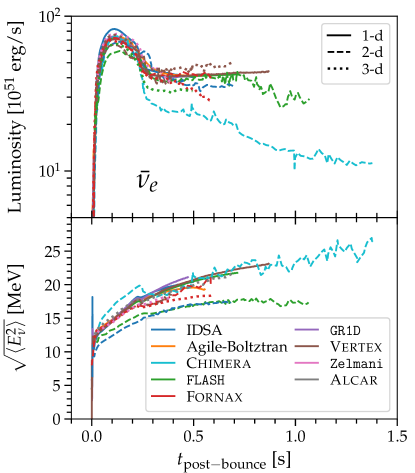
Figure 1: Neutrino ($\bar{\nu}_{e}$; others shown in S.M.) luminosity and RMS energy profiles from supernova simulations O’Connor et al. (2018); Bruenn et al. (2013, 2016); O’Connor and Couch (2018a); Summa et al. (2016); Kotake et al. (2018); Vartanyan et al. (2018); Ott et al. (2018); O’Connor and Couch (2018b); Glas et al. (2019); Burrows et al. (2020).

Comparing models.— We first consider the nominal case of a 20$M_{\odot}$ progenitor and no neutrino oscillations. For all modern 1-, 2-, and 3-d models O’Connor et al. (2018); Bruenn et al. (2013, 2016); O’Connor and Couch (2018a); Summa et al. (2016); Kotake et al. (2018); Vartanyan et al. (2018); Ott et al. (2018); O’Connor and Couch (2018b); Glas et al. (2019); Burrows et al. (2020), we collect information on their neutrino fluxes and spectra. We seek to assess the full variation between models, though they are not completely distinct, e.g., many share progenitors Woosley and Heger (2007). These models vary significantly in their sophistication in various aspects, but we do not attempt to adjudicate between them. Most multi-d models lead to successful explosions, with explosion times ranging from 0.2–0.8 s. The model details are given in S.M.

Figure 1 shows their time profiles of $\bar{\nu}_{e}$ luminosity and root-mean-square (RMS) energy (other flavors are shown in S.M.). For the spectra, we assume a commonly used form, $f_{\alpha}(E_{\nu})=\mathcal{N}\left({E_{\nu}}/{\langle E_{\nu}\rangle}\right)^{\alpha-2}e^{-(\alpha+1)E_{\nu}/\langle E_{\nu}\rangle}$, where $\langle E_{\nu}\rangle$ is the average energy and $\alpha$ sets the spectrum shape Keil et al. (2003). Different groups characterize spectra differently, and we show how we correct for this in S.M.

To model the detected spectra, we follow standard calculations (see, e.g., Refs. Jegerlehner et al. (1996); Lunardini and Smirnov (2004); Costantini et al. (2007); Pagliaroli et al. (2009); Vissani (2015)) and give details in S.M. The dominant process is $\bar{\nu}_{e}+p\rightarrow e^{+}+n$ with free (hydrogen) protons, for which we take the cross sections and kinematics from Refs. Vogel and Beacom (1999); Strumia and Vissani (2003). To model the detectors, we take into account their fiducial masses, energy resolutions, and trigger efficiencies Hirata et al. (1987, 1988); Bionta et al. (1987); Bratton et al. (1988). Because of the different detector responses, the detected positron energies are expected to be significantly lower for Kam-II than IMB. For the distance of SN 1987A, we use 51.4 kpc Panagia (1999).

We compare the predicted and observed SN 1987A neutrino data using simple, robust observables and statistical tests. We conduct goodness-of-fit tests (computing p-values) between pairs of models and between each model and the SN 1987A data. Because we are testing goodness-of-fit, rather than doing parameter estimation, maximum likelihood is not a suitable method; see S.M.

The main panels of Figs. 2–4 show simple visual comparisons of the counts and average detected energies. For consistency, here we cut off all models at 0.5 s. Because we forward-model the theoretical predictions (taking into account properties of the individual detectors and Poisson fluctuations), the full error bars (see S.M. for details) are shown on the predictions.

The insets of Figs. 2–4 show our main statistical calculations. Larger p-values indicate agreement; we define $p<0.05$ as indicating inconsistency for a given model, though our main focus is on what happens for the majority of models. Here we allow each model to go to its full run time (typically 0.5–1.5 s). For these, we consider both the counts in the time profile and the shape of the energy spectrum. Given the short timescale and the low statistics, we treat these separately. For the counts tests, the p-values are the one-sided cumulative Poisson probabilities. For the spectrum tests, we use one-dimensional Kolmogorov-Smirnov statistics, following Monte Carlo modeling of the predicted data. We allow free time offsets between the predictions and the data for each detector, finding that these values are $\simeq$0.1 s for Kam-II and $\simeq$0.2 s for IMB, both small, so this freedom does not affect our results.

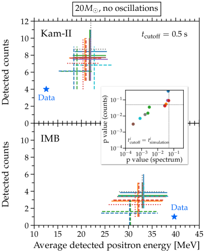
Figure 2: Predicted counts and average energies of supernova models (colors as in Fig. 1), compared to each other and to SN 1987A data. Our main calculations are in the inset.

Results for the Nominal Case.— Figure 2 shows the model-to-model comparisons for a 20$M_{\odot}$ progenitor with no neutrino oscillations. The p-values obtained by comparing pairs of models range over 0.06–0.52 for the counts (Kam-II and IMB combined) and 0.03–0.99 for the spectra (Kam-II only, as IMB has too few counts). A general consistency in both the predicted counts and spectra is evident. Considering the range and complexity of the inputs and methods in supernova modeling, this agreement is encouraging, though it remains important to understand the residual differences.

Figure 2 also shows the model-to-data comparisons. A general inconsistency in both the counts and spectra is evident. The predicted counts are too high for Kam-II and mostly too high for IMB. The predicted average detected energies are too high for Kam-II and slightly too low for IMB (because IMB has just one detected event in this time range, we do not use the predicted spectrum in our statistical tests). Quantitatively, no model-to-data comparisons have both p-values larger than 0.05, and many are much worse. To confidently interpret data from the next Milky Way supernova, multiple simulations that can reproduce the neutrino and electromagnetic data will be a must. Confidence in this would greatly increase if the same were achieved for SN 1987A.

Possible Solutions: Neutrino Oscillations.— The detected supernova neutrino data are affected by neutrino oscillations Duan et al. (2010); Mirizzi et al. (2016); Horiuchi and Kneller (2018); Tamborra and Shalgar (2021); Capozzi and Saviano (2022); Richers and Sen (2022), with the effects depending upon differences in the initial neutrino luminosities and spectra, set by differences in their production processes and opacities. The details depend on the high densities of matter and other neutrinos, which are uncertain Mirizzi et al. (2016). Generally, matter-induced effects occur in the stellar envelope Dighe and Smirnov (2000), while neutrino-induced effects occur just outside the neutrinospheres Tamborra and Shalgar (2021); Capozzi and Saviano (2022); Richers and Sen (2022).

We study the effects of oscillations with a few representative cases. Considering only matter-induced effects, if the neutrino mass ordering follows the inverted hierarchy (IH), then there can be a nearly complete exchange of the $\bar{\nu}_{e}$ and $\bar{\nu}_{x}$ ($\bar{\nu}_{\mu}$ and $\bar{\nu}_{\tau}$) flavors, with almost no change for the $\nu_{e}$ and $\nu_{x}$ flavors Dighe and Smirnov (2000). In the normal hierarchy (NH), the opposite occurs. With neutrino-induced effects, it is possible to have nearly complete equilibration of all six flavors soon after decoupling, because of rapid flavor conversions induced by interactions of neutrinos among themselves Tamborra and Shalgar (2021); Capozzi and Saviano (2022); Richers and Sen (2022). Further details are given in S.M.

Figure 3 shows the effects of example neutrino-oscillation scenarios (all for the Alcar 3-d Glas et al. (2019) model and a 20$M_{\odot}$ progenitor, chosen because it is 3-d and has a long runtime). In general, oscillations decrease the predicted counts and increase the average energies, as $\bar{\nu}_{x}$ has lower fluxes but higher energies than $\bar{\nu}_{e}$. For most simulations (including this model), the reduction in flux is more significant. The correlated trend in how the spectrum p-value changes relative to the counts p-value is due to finite statistics and is explained in S.M. In effect, only one p-value matters, and that is the one for the spectrum. Last, as an overall trend, models with longer simulation times tend to disagree more with data, as shown via the grey symbols in the inset.

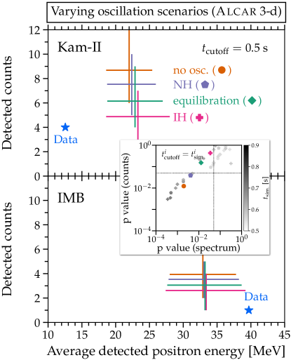
Figure 3: Similar to Fig. 2, with the theory predictions from the Alcar 3-d model for 20 $M_{\odot}$ Glas et al. (2019) and different oscillation scenarios. The simulation cutoff time is 0.68 s. The grey symbols show the p-values from other simulation groups. See S.M. for details.

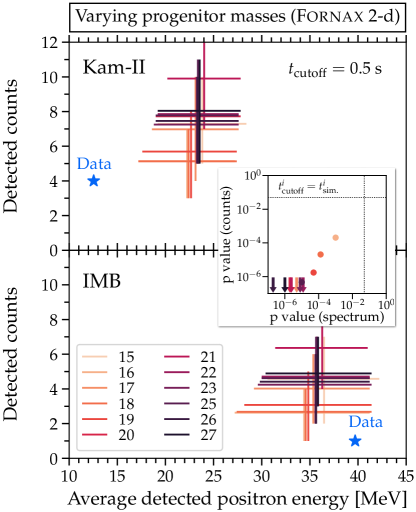
Figure 4: Similar to Fig. 2, with the theory predictions corresponding to different progenitors from Fornax 2-d models Burrows and Vartanyan (2021), with no oscillations included.

Possible Solutions: Supernova Progenitors.— The detected supernova neutrino data are also affected by the choice of progenitor Woosley et al. (1986); O’Connor and Ott (2013). The structure of the star at collapse determines the accretion rate onto the PNS, which strongly influences the neutrino emission. A key question is if models with progenitors other than the 20$M_{\odot}$ single-star cases considered above would better fit the SN 1987A data.

Figure 4 shows the effects of different choices of progenitor mass, using the suite of Fornax 2-d models in Ref. Burrows and Vartanyan (2021), chosen because of their wide range of progenitor masses (we use 16–30$M_{\odot}$) and long runtimes. None of the progenitors provides a good fit to the data. We have also carried out this analysis (see selected results in S.M.) for the suites of models from Refs. Summa et al. (2016); Vartanyan et al. (2019a); Burrows et al. (2019); Vartanyan et al. (2019b); Nagakura et al. (2019); Burrows et al. (2020); Warren et al. (2020); Baxter et al. (2022), again finding poor agreement with data.

The lack of good agreement between models and SN 1987A data may indicate missing physics. Softening the predicted neutrino spectra (which would also reduce the predicted counts) would require changing the thermodynamic structure of the outer layers of the PNS or changing the neutrino opacity in those regions. (Although supernova neutrinos may not be emitted isotropically Tamborra et al. (2014); Takiwaki and Kotake (2018); Lin et al. (2020); Walk et al. (2019), the predicted effects on the number flux are less than $\pm 20$% and those on the average energy are even less, both too small to explain the observed discrepancies.) However, it may just be that there are not enough models. There are not many studies of the same progenitors with different simulation codes, and there are also not many different progenitors in use. Additionally, binary-merger models for the progenitor of SN 1987A (which do not clearly map onto single-star models) are needed, but only Ref. Nakamura et al. (2022) provides neutrino predictions. A broad range of new simulation work on progenitors and core collapse is needed, especially combining both high sophistication and long runtime. A big step in that direction is made in Ref. Bollig et al. (2021) (for $19M_{\odot}$), but which we find gives a comparably poor match to the SN 1987A data.

Conclusions and Ways Forward.— The SN 1987A neutrino and electromagnetic data, which reasonably agreed with supernova models of the time, have been of critical importance to our understanding of core-collapse supernovae. It is commonly assumed that modern supernova models — with 36 years of improvements — also match the data. We revisit this assumption.

We show that most modern models (for a $20M_{\odot}$ progenitor and no neutrino oscillations) disagree with 1987A neutrino data in the first $\simeq$0.5–1.5 s, where the highest-precision models end. Compared to the Kam-II data, these models predict higher counts and higher average energies. Compared to the IMB data, these models generally predict higher counts (as noted, we do not use their average energies, which means that our results do not depend on the well-known spectrum tension between Kam-II and IMB). When we include the effects of various neutrino-oscillation scenarios, the predicted counts become lower and the average energies become slightly higher, so that the tension with data remains. When we vary the progenitor mass, the trend is not monotonic, but the tension with data again remains. Finally, as can be seen from comparing Figs. 3 and 4, varying the oscillation scenario and the progenitor together would not resolve the tensions with data.

We also show that most modern models are in good agreement with each other, which suggests that there may be a common solution to the disagreement with SN 1987A data, perhaps even one that also improves explosion energies in simulations. There is a range of possibilities, including that our implementation or even understanding of the physics in the simulations is incomplete, that not enough progenitor models have been considered, that the initial neutrino spectra are nonthermal (e.g., Refs. Yuksel and Beacom (2007); Nagakura and Hotokezaka (2021)), or that neutrino oscillations need to be directly implemented in supernova simulations Ehring et al. (2023). Separately, it would also be interesting to reanalyze the raw data from both detectors, using present detector-modeling and event-reconstruction techniques, both vastly improved over those from 36 years ago.

To realize the full potential of observing and interpreting the signals from the next Milky Way supernova, the community will ultimately need a set of modern models that agree (for the same progenitor mass) with each other and the neutrino and electromagnetic data. An important step towards that is seeking the same for SN 1987A. Reaching these goals should be pursued with urgency. It is especially important that multi-d supernova simulations push their run times out to a few seconds, beyond which PNS cooling simulations may be adequate.

Acknowledgments.— We are grateful for helpful discussions with Benoît Assi, Elias Bernreuther, Adam Burrows, Nikita Blinov, Basudeb Dasgupta, Sebastian Ellis, Ivan Esteban, Chris Fryer, Christopher Hirata, Josh Isaacson, Thomas Janka, Daniel Kresse, Gordan Krnjaic, Bryce Littlejohn, Sam McDermott, Alessandro Mirizzi, Masayuki Nakahata, Evan O’Connor, Ryan Plestid, Georg Raffelt, Prasanth Shyamsundar, Michael Smy, and especially Pedro Machado. We acknowledge the use of the KS2D code. S.W.L. was supported at FNAL by the Department of Energy under Contract No. DE-AC02-07CH11359 during the early stage of this work. J.F.B. was supported by NSF Grant No. PHY-2012955.

Supplemental Material for

Old Data, New Forensics: The First Second of SN 1987A Neutrino Emission

Shirley Weishi Li, John F. Beacom, Luke F. Roberts, and Francesco Capozzi

Here we provide additional details that may be useful. Appendix A summarizes key aspects of the supernova models, Appendix B shows the 1987A data we use, Appendix C focuses on how the average energy and spectrum parameter are calculated for each model, Appendix D explains the calculation of the detected positron energy spectra, Appendix E provides details about the statistical tests, Appendix F presents results on progenitor variations, and Appendix G shows details of the oscillation calculations.

Appendix A Supernova simulations

Code	Dimension	Progenitor Mass [$M_{\odot}$]	Explosion	$t_{\mathrm{exp}}$ [s]	$t_{\rm sim}$ [s]	p-value (counts)	p-value (spectra)	Reference
3DnSNe-IDSA	1-d	20 Woosley and Heger (2007)	N/A	N/A	0.50	0.043	0.027	O’Connor et al. O’Connor et al. (2018)
AGILE-BOLTZTRAN					0.55	0.055	0.034
FLASH-M1					0.71	0.015	0.002
Fornax					1.10	–	–
GR1D					0.47	0.092	0.043
Prometheus-Vertex					0.87	0.003	3$\times 10^{-4}$
Chimera	2-d	20 Woosley and Heger (2007)	Yes	0.21	1.37	0.007	7$\times 10^{-4}$	Bruenn et al. Bruenn et al. (2013, 2016)
FLASH	2-d	20 Woosley and Heger (2007)	Yes	0.82	1.06	0.035	0.003	O’Connor et al. O’Connor and Couch (2018a)
Prometheus-Vertex	2-d	20 Woosley and Heger (2007)	Yes	0.36	0.38	–	–	Summa et al. Summa et al. (2016)
IDSA	2-d	20 Woosley and Heger (2007)	Yes/No	0.4–0.6	0.68	0.35	0.047	Kotake et al. Kotake et al. (2018)
Fornax	2-d	20 Woosley and Heger (2007)	No	N/A	0.58	0.042	0.029	Vartanyan et al. Vartanyan et al. (2018)
Zelmani	3-d	20 Woosley and Heger (2007)	Yes	0.38	0.38	–	–	Ott et al. Ott et al. (2018)
FLASH	3-d	20 Farmer et al. (2016)	No	N/A	0.50	–	–	O’Connor et al. O’Connor and Couch (2018b)
Alcar	3-d	20 Woosley and Heger (2007)	No	N/A	0.68	0.012	0.002	Glas et al. Glas et al. (2019)
Fornax	3-d	20 Sukhbold et al. (2016)	Yes	0.45	0.59	0.091	0.047	Burrows et al. Burrows et al. (2020)

Table S1: A summary of the supernova simulations considered. The progenitor mass refers to the zero-age main sequence mass. We take the explosion time to be the moment when the mean shock radius reaches 500 km. The p-values are obtained from the comparison between the model predictions and SN 1987A data. The p-values in the counts column are from comparing the total number of events in Kam-II and IMB. Those in the spectrum column are from comparing the cumulative spectrum distribution in Kam-II only (because IMB has too few counts). See the text for why some models do not have p-values.

Table S1 summarizes the list of supernova models employed in this work. The p-values are computed up to the maximum time in each simulation. We exclude four models from our statistical tests: the 1-d Fornax models from Ref. O’Connor et al. (2018) that have a known bug Burrows , a FLASH 3-d simulation paper O’Connor and Couch (2018b) that reports neutrino luminosities but not average energies, and the Prometheus-Vertex 2-d Summa et al. (2016) and Zelmani 3-d Ott et al. (2018) simulations, which only run to 0.38 s.

Appendix B SN 1987A data

Tables S2 and S3 show the 1987A events in Kam-II and IMB that we used in this work. Note that there are later detected events that we did not include because they are after the longest simulation time that we consider, $\simeq 4.6$ s.

Event	Time [s]	Energy [MeV]
1	0.000	20.0
2	0.107	13.5
3	0.303	7.5
4	0.324	9.2
5	0.507	12.8
6	1.541	35.4
7	1.728	21.0
8	1.915	19.8

Table S2: Kam-II data taken from Ref. Hirata et al. (1988). The event energy is the total energy of the detected positron.

Event	Time [s]	Energy [MeV]
1	0.000	38
2	0.412	37
3	0.650	28
4	1.141	39
5	1.562	36
6	2.684	36

Table S3: IMB data taken from Ref. Bratton et al. (1988). The event energy is the total energy of the detected positron.

Appendix C Neutrino energy spectra and luminosities

Figure S1 shows the time evolution of luminosity and root-mean-square (RMS) energy for all flavors and for each model. It is evident by eye that there is relatively good agreement, with some exceptions. Most of these quantities are taken directly from publications, but some require a conversion from average energies, $\langle E_{\nu}\rangle$, to root-mean-square energies, $\sqrt{\langle E^{2}_{\nu}\rangle}$. Some require changing from the fluid frame to an infinite observer frame.

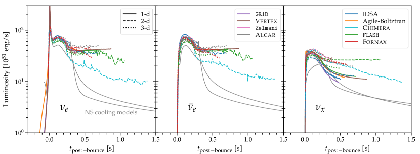
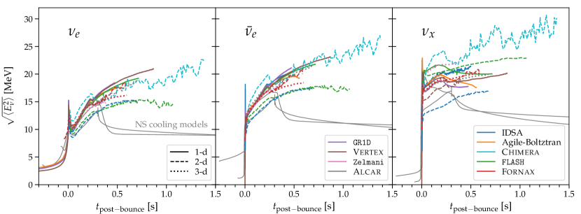
Figure S1: Neutrino luminosities (top) and RMS energies (bottom) of $\nu_{e}$, $\bar{\nu}_{e}$, and $\nu_{x}$ from numerical simulations. The neutronization burst luminosity goes up to $\simeq 5\times 10^{53}$erg/s. The $\nu_{x}$ luminosity is shown for only one of the four flavors. The two PNS cooling models are from Refs. Nakazato et al. (2013); Roberts and Reddy (2016).

Our calculations require the full neutrino energy distribution function, $f(E_{\nu})$, which is assumed to be already integrated over neutrino propagation angle. Sometimes the output $f(E_{\nu})$ from a given model is publicly released, usually in the form of large numerical tables. However, this is available only for very few models. Fortunately, in Ref. Keil et al. (2003), a good analytical approximation for $f(E_{\nu})$ has been found (we include the $E_{\nu}^{2}$ factor in the phase-space integral, not the distribution function):

$$f(\alpha,E_{\nu})=\mathcal{N}\left(\frac{E_{\nu}}{\langle E_{\nu}\rangle}\right)^{\alpha-2}e^{-\frac{(\alpha+1)E_{\nu}}{\langle E_{\nu}\rangle}},$$ (1)

where $\langle E_{\nu}\rangle$ is the average neutrino energy, defined as

$$\langle E_{\nu}\rangle=\frac{\int_{0}^{\infty}dE_{\nu}\,E_{\nu}^{3}f(E_{\nu})}{\int_{0}^{\infty}dE_{\nu}\,E_{\nu}^{2}f(E_{\nu})}\,,$$ (2)

and $\alpha$, representing the amount of spectrum pinching, is defined as

$$\frac{\langle E_{\nu}^{2}\rangle}{\langle E_{\nu}\rangle^{2}}=\frac{2+\alpha}{1+\alpha}\,,$$ (3)

and $\mathcal{N}$ is a normalization factor that ensures the distribution function integrates to the local neutrino number density. For a Fermi-Dirac distribution with zero chemical potential, we have $\langle E_{\nu}\rangle\simeq 3.15T$, where $T$ is the temperature, and $\sqrt{\langle E_{\nu}^{2}\rangle}=1.14\langle E_{\nu}\rangle$.

The pinched spectrum $f(\alpha,E_{\nu})$ defined in Eq. (1) is what we use to calculate the theoretical predictions for SN 1987A. We need both $\langle E_{\nu}\rangle$ and $\sqrt{\langle E_{\nu}^{2}\rangle}$, but some models only provide one of them, either through numerical tables or figures. To solve this lack of information, we fit for a simple relation between $\langle E_{\nu}\rangle$ and $\sqrt{\langle E_{\nu}^{2}\rangle}$ using the models that provide both. Figure S2 shows $\sqrt{\langle E_{\nu}^{2}\rangle}$ as a function of $\langle E_{\nu}\rangle$ for these models. Most models predict $\sqrt{\langle E_{\nu}^{2}\rangle}$ to be between 1.08$\langle E_{\nu}\rangle$ and 1.13$\langle E_{\nu}\rangle$ in the energy range 12–20 MeV, where the average energies of most models fall. Thus, we adopt the following relation between average and root-mean-square neutrino energy

$$\sqrt{\langle E_{\nu}^{2}\rangle}=1.025\langle E_{\nu}\rangle+0.005\langle E_{\nu}\rangle^{2}\,,$$ (4)

which fits most of the models well, and is at most 10% away from the Fornax results. Equation (4) is then used to compute a relation between $\alpha$ and $\langle E_{\nu}\rangle$.

Note that some groups define $E_{\text{rms}}=\sqrt{\langle E_{\nu}^{3}\rangle/\langle E_{\nu}\rangle}$ as opposed to $E_{\text{rms}}=\sqrt{\langle E_{\nu}^{2}\rangle}$. We find that taking this into account leads to negligible changes to the predicted event rates, so we interpret all RMS energies as $\sqrt{\langle E_{\nu}^{2}\rangle}$.

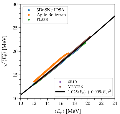
Figure S2: $\sqrt{\langle E_{\nu}^{2}\rangle}$ as a function of $\langle E_{\nu}\rangle$ obtained from the numerical simulations where both are provided. The black line is the relation we use in this work.

Some models provide neutrino predictions in the comoving frame of the stellar fluid. However, we need quantities defined in the laboratory frame. We use the transformations between these frames from Ref. Kotake et al. (2018). For the neutrino luminosity, the transformation reads:

$$L_{\nu}=L_{\nu}^{\mathrm{fluid}}(1+v_{r}/c)/(1-v_{r}/c)\,,$$ (5)

and for the average energy, it is

$$\sqrt{\langle E_{\nu}^{2}\rangle}=\sqrt{\langle E_{\nu}^{2}\rangle^{\mathrm{fluid}}}(1+v_{r}/c)/\sqrt{1-(v_{r}/c)^{2}},$$ (6)

with $v_{r}$ being the radial velocity and $c$ the speed of light. In Ref. Kotake et al. (2018), it is assumed $v_{r}=-0.06c$, which is the average infall velocity at 500 km over the entire 250 ms post bounce. Considering that the transformation between frames is at the level of $O(10\%)$, our approximation can be safely applied to all models.

Appendix D Detected positron energy spectrum

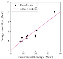
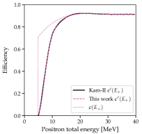
Figure S3: (Left) The black dots represent the energy uncertainty for each event detected in Kam-II, whereas the continuous line is a fit to this data; we use the fit to get the width of the Gaussian energy resolution function defined in the text. (Right) The efficiency of Kam-II as a function of the true positron total energy. Note that our calculation perfectly overlaps the line provided by Kam-II.

We follow the standard approach to compute the positron spectrum Jegerlehner et al. (1996); Lunardini and Smirnov (2004); Costantini et al. (2007); Pagliaroli et al. (2009); Vissani (2015). As a first step to predicting the detected positron energy spectrum, we calculate the spectrum as a function of the true positron total energy $E_{+}$:

$$g(E_{+})\propto\int dE_{\nu}E_{\nu}^{2}f(\langle E_{\nu}\rangle,\alpha)\frac{d\sigma_{\mathrm{IBD}}(E_{\nu},E_{+})}{dE_{+}}\,,$$ (7)

where $d\sigma_{\mathrm{IBD}}/dE_{+}$ is the differential cross section for the inverse beta decay Vogel and Beacom (1999); Strumia and Vissani (2003) and $f(\langle E_{\nu}\rangle,\alpha)$ is defined in Eq. (1).

To turn $g(E_{+})$ into an observed spectrum, we need to convolve it with the detector energy resolution and efficiency. We detail the Kam-II case. The trigger has a threshold of $N_{\mathrm{hit}}\geq 20$ (the number of hit photomultiplier tubes), which is equivalent (on average) to a detected energy, $E_{\mathrm{det}}$, of 7.5 MeV. The detected spectrum is then

$$N(E_{\mathrm{det}})\propto\int dE_{+}g(E_{+})\epsilon(E_{+})R(E_{\mathrm{det}},E_{+})\theta(E_{\mathrm{det}}-7.5),$$ (8)

where $\epsilon(E_{+})$ is the intrinsic detector efficiency (not taking into account the $E_{\mathrm{det}}$ cut), $R(E_{\mathrm{det}},E_{+})$ is the energy resolution function and $\theta(E_{\mathrm{det}}-7.5)$ is the Heaviside step function. We assume $R(E_{\mathrm{det}},E_{+})$ to be a Gaussian function, with the width $\sigma_{R}$ having the form $aE_{+}+b\sqrt{E_{+}}$, where the second term arises from the Poisson fluctuations on $N_{\rm hit}$, while the first term roughly accounts for systematics. The black dots in Fig. S3 (left panel) represent the energy errors of each event detected in Kam-II Hirata et al. (1988). We obtain the following expression for the width from a functional fit:

$$\sigma_{R}^{\mathrm{KamII}}(E_{+})=0.18E_{+}+0.14\sqrt{E_{+}}\,.$$ (9)

The published trigger efficiency curve from Fig. 3 of Ref. Hirata et al. (1988) should be interpreted as $\epsilon^{\prime}(E_{+})$, combining the intrinsic detector efficiency and the trigger cut:

$$\epsilon^{\prime}(E_{+})=\epsilon(E_{+})\int dE_{\mathrm{det}}R(E_{\mathrm{dec}},E_{+})\theta(E_{\mathrm{det}}-7.5)\,.$$ (10)

Figure S3 (right panel) shows the trigger efficiency we have computed (pink dashed line) in comparison with the one published by Kam-II (black solid line), which match perfectly. In addition, we also show the inferred intrinsic efficiency $\epsilon(E_{+})$ with the dotted line.

A similar procedure has been applied for IMB. Figure S4 displays both the energy resolution (left panel) and the efficiency (right panel) extracted for this experiment.

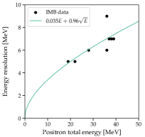
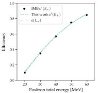
Figure S4: Same as Fig. S3, but for IMB, which only provides efficiencies at a few energy points.

Appendix E Statistical methods

E.1 Calculating time offset

As the supernova neutrinos reach Earth, the expected number of events increases as a function of time because the supernova signal is rising. However, due to the limited statistics, the first detected event is generally expected to occur at 0.1–0.2 s after the neutronization burst peak. In addition, because the two detectors, KamII and IMB did not record the absolute time difference of their respective first events, this time offset has to be applied separately to KamII and IMB.

The method we use for calculating the offset time is the following. First, we look only at data as a function of time, and we discard energy information. For example, let us consider one simulation running up to 0.6 s. Let us also assume that KamII data has the following detection times for each event: $(0.0,0.1,…,t_{n})$ s. We test offsets in the range $[0,0.5]$ s. For every offset ($t_{0}$), the detection times with respect to the arrival of the neutronization peak, which can be taken as $t=0$ in simulations, become $(0.0+t_{0},0.1+t_{0},…,t_{n}+t_{0})$. Next, we compute the p-value as $P_{1}\times P_{2}$, where $P_{1}$ is the Poisson probability of predicting $N$ events and getting $N^{\prime}$ events, i.e., what we quote as the p-value for rates. $P_{2}$ is the Kolmogorov-Smirnov test p-value obtained by comparing the detected and predicted temporal shapes (see Fig. S5 left panel for the spectrum example). We get an array of p-values, one for each value of $t_{0}$. We choose the time offset for which the p-value is maximal. In general, in the plausible range of time offset, i.e., $[0.1,0.2]$ s, the p-value is rather constant because the data is sparse, and we are not including more events to KamII data when shifting the time. Concerning IMB, the number of events can change for some models, which we do use when computing p-values. However, their number would still be so low that their contribution to the combined p-value is only marginal.

E.2 Cumulative distributions and Kolmogorov-Smirnov test

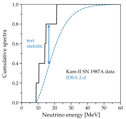
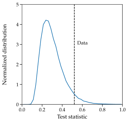
Figure S5: A demonstration of p-value calculation. (Left) The cumulative energy distribution of the IDSA 2-d model and 1987A data and the corresponding test statistic. (Right) The test statistic distribution.

To compute the p-values for the spectrum shape, we use a Kolmogorov-Smirnov test. Figure S5 (left panel) illustrates the test statistic. We use one specific model, IDSA 2-d Kotake et al. (2018), as a concrete example. First, we utilize all the available information and set $t_{\text{cutoff}}$ to be the simulation run time, 0.67 s for this model. We then integrate the energy spectrum up to $t_{\text{cutoff}}$ and plot the cumulative distribution (blue dashed line). Next, we cut the 1987A Kam-II data also at $t_{\text{cutoff}}$, allowing a variable offset time. The black steps show the cumulative spectrum of the data within 0.67 s. The test statistic is the maximum vertical distance between these two curves, TS₀.

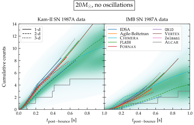
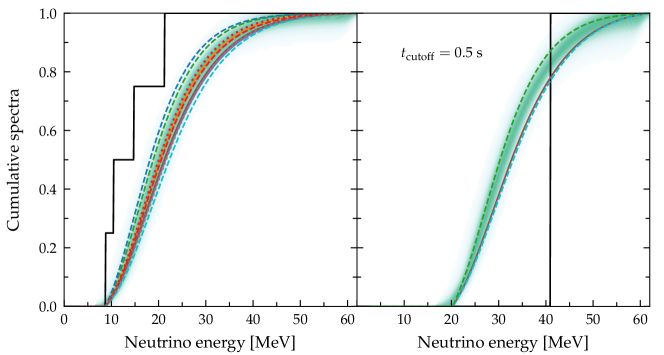
Figure S6: Cumulative counts (top panel) and cumulative spectra (bottom panel) of models compared to SN 1987A data. The green shading shows the density of all models considered in this work, including the alternative scenarios with neutrino oscillation and different progenitor masses.

To compute p-values, we run Monte Carlo simulations of each detector to build the test statistic distribution, shown in Fig. S5 (right panel). For this model, we sample many realizations of the data, letting both the total counts and the energy points vary, and compute the test statistic between the model and each realization. The p-value is determined by the fractional area of the p-value distribution more extreme than TS₀.

This Monte Carlo sample is also used to compute the error bars in Figs. 2–4. The vertical error bars follow Poisson fluctuations, as expected. The horizontal error bars are the standard deviation of the mean for the detected positron energies in each detector. As noted in the main text, the results shown in the main panels of those figures are simple visual comparisons, with the insets showing our full statistical calculations.

Figure S6 (top panel) shows how the cumulative counts for the models compare to 1987A data. The green shading indicate smearing over all models, including those for different oscillation scenarios and progenitor masses in Ref. Warren et al. (2020). Here we clearly see the trend of models predicting too high of event counts throughout the entire 1 s. Figure S6 (bottom panel) shows the cumulative energy spectra of all models, and similarly, the green shading indicate the model range.

One may be tempted to use likelihood as a test statistic to compute p-values. Here we follow the discussions in Ref. James (2006) (Chapter 11) and explain why this is not a robust statistical procedure. The essential point is that we are doing a goodness-of-fit test, and not a model comparison or parameter estimation. While maximum likelihood is a good method for model comparison or parameter estimation, it does not work as a goodness-of-fit test, regardless of whether one works in the frequentest or Bayesian framework. A simple demonstration of why is to consider a uniform distribution $h(x)=1$ between (0, 1), where we want to test whether some random numbers $\{x_{i}\}$ are drawn from the uniform distribution. Clearly any data set would generate a likelihood of 1, so this fails as a goodness-of-fit test. The lesson is generically applicable to other distributions because we can always transform a smooth distribution to a uniform one by changing variables.

Appendix F Progenitors from different groups

In Fig. 4, we show a comparison between model predictions and data for different values of the progenitor mass, but only for Fornax 2-d. Here we provide further details.

Figure S7 shows the cumulative distributions for different progenitors by FLASH 1-d Warren et al. (2020) compared to 1987A data Baxter et al. (2022). This is the study with the largest suites of progenitor models. Because of the huge number of models, we decide not to label any specific progenitors but rather focus on some general points. First, there are clearly two families of curves, one with steeply rising event rates and one with flattening event rates beyond $\simeq$ 0.5 s. The first family corresponds to models where the supernova failed to explode and the second to successful explosions. Interestingly, models with successful explosions are thus closer to the SN 1987A data. This means there may be a strong connection between the two questions “Does the model explode?” and “Does the model match the data?” Further exploration of that conjecture is needed.

Combining results from all groups with long-term simulations of a range of progenitor models, Fig. S8 (left panel) shows how the p-values for the energy spectrum comparison of FLASH Warren et al. (2020), Vertex Summa et al. (2016) and Fornax Burrows and Vartanyan (2021) change with the progenitor mass in 10–80$M_{\odot}$. This panel assumes a cutoff time of $t_{\rm cutoff}=0.5$ s. In this case, most of the p-values lie above the dashed line that represents our $p=0.05$ threshold. Then most of these models appear to be in agreement with data, especially in the range 10–20$M_{\odot}$. On the other hand, the right panel uses $t_{\rm cutoff}=1.3$ s. In this case, a general disagreement with data is clearly visible. We stress that the choice of $t_{\rm cutoff}=0.5$ s is only to make the time range for each simulation equal. It is unsurprising that restricting the time range lessens the statistical tension. The p-values for the case where $t_{\rm cutoff}$ is equal to the cutoff time of each simulations are the ones to be taken as references, since ultimately we would like all simulations to agree with data for the entire duration of the neutrino burst.

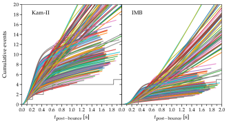
Figure S7: Cumulative numbers of events for different progenitors simulated with FLASH 1-d Warren et al. (2020).

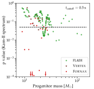
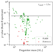
Figure S8: The p-values obtained through an energy spectrum comparison with Kam-II data for different progenitors masses, simulated with FLASH Warren et al. (2020), Vertex Summa et al. (2016) and Fornax Vartanyan et al. (2019a); Burrows et al. (2019); Vartanyan et al. (2019b); Nagakura et al. (2019); Burrows et al. (2020); Burrows and Vartanyan (2021), with a cutoff time of 0.5 s (left) and 1.3 s (right).

Appendix G Supernova neutrino oscillation treatment

We consider a few illustrative oscillation scenarios in the main text, focusing on exploring the possible impact of oscillations on the model-data comparison. We use the following equation for calculating the oscillated flux $\tilde{f}_{\bar{\nu}_{e}}$ of $\bar{\nu}_{e}$ as a function of the unoscillated fluxes.

$$\tilde{f}_{\bar{\nu}_{e}}=f_{\bar{\nu}_{e}}P(\bar{\nu}_{e}\to\bar{\nu}_{e})+f_{\bar{\nu}_{x}}[1-P(\bar{\nu}_{e}\to\bar{\nu}_{e})]\,,$$ (11)

where $P(\bar{\nu}_{e}\to\bar{\nu}_{e})=\cos^{2}\theta_{12}\simeq 0.7$ in NH, $P(\bar{\nu}_{e}\to\bar{\nu}_{e})=0$ in IH and $P(\bar{\nu}_{e}\to\bar{\nu}_{e})=\frac{1}{3}$ for flavor equilibration.

In Figs. S9 to S12, we show the effects of oscillations on the predicted event rates, spectra, and p-values for models from different groups. For simulations with the same dimensions, we sort the results in ascending order of simulation time. While some models have reasonable p-values, in general the fit worsen as the simulation time increases; when the runtimes are short, models can appear better than they likely are. This point seems to be confirmed by the results of Ref. Bollig et al. (2021) (for $19M_{\odot}$), a sophisticated model with a long runtime, which also gives a poor match to the SN 1987A data. It would be desirable to have more models that run longer. Finally, the goal is to have nearly all models fit the data well.

There is a nontrivial interplay between the p-values for the counts and spectra. As an example, let us consider the Alcar 3-d results, as shown in the main text in Fig. 3. Oscillations convert $\bar{\nu}_{x}$ and $\bar{\nu}_{e}$ into each other, which means that the detected $\bar{\nu}_{e}$ spectrum has a lower number of neutrinos and an increased average energy with respect to the one at production. Because without oscillations theoretical predictions give a higher flux compared to data, their inclusion makes the counts p-value better. On the other hand, the unoscillated value of the average energy for $\bar{\nu}_{e}$ is higher than that the observed one in the Kam-II data, thus oscillations should, in principle, make the spectrum p-value worse. But the opposite happens because the spectrum p-value includes information on counts in a subtle way. To explain why, let us look at Fig. S5. If we increase the predicted average energy, the predicted spectrum (blue dashed line in the left panel) shifts to the right, increasing the test statistic relative to data. However, to calculate a p-value for a test statistic, we run Monte Carlo samples based on the blue dashed curve. With oscillations, because of the lower flux, we would generally sample fewer events for the mock data samples, which would increase the mock test statistic because of the coarse steps. In combination, it is not clear whether the spectrum p-value would increase or decrease, but what seems to happen in most of the models is that the spectrum p-values end up increasing because they are dominated by the bad fit due to the counts.

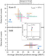
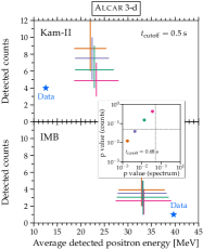
Figure S9: Different oscillation scenarios for 3-d simulations.

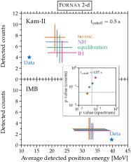
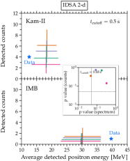
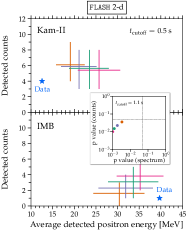
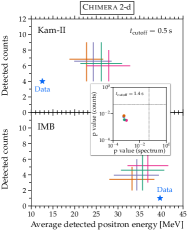
Figure S10: Different oscillation scenarios for 2-d simulations.

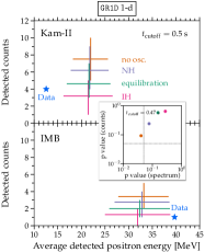
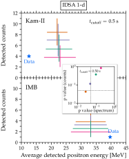
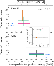
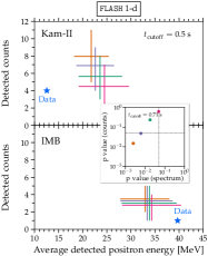
Figure S11: Different oscillation scenarios for 1-d simulations.

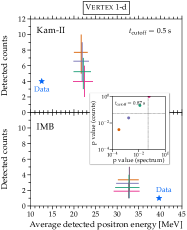
Figure S12: Figure S11 continued.

References

- Hirata et al. (1987) K. Hirata et al. (Kamiokande-II), “Observation of a Neutrino Burst from the Supernova SN 1987a,” Phys. Rev. Lett. 58, 1490–1493 (1987).
- Hirata et al. (1988) K. S. Hirata et al., “Observation in the Kamiokande-II Detector of the Neutrino Burst from Supernova SN 1987a,” Phys. Rev. D 38, 448–458 (1988).
- Bionta et al. (1987) R. M. Bionta et al., “Observation of a Neutrino Burst in Coincidence with Supernova SN 1987a in the Large Magellanic Cloud,” Phys. Rev. Lett. 58, 1494 (1987).
- Bratton et al. (1988) C. B. Bratton et al. (IMB), “Angular Distribution of Events From Sn1987a,” Phys. Rev. D 37, 3361 (1988).
- Arnett et al. (1989) W. D. Arnett, John N. Bahcall, R. P. Kirshner, and S. E. Woosley, “Supernova 1987A,” Ann. Rev. Astron. Astrophys. 27, 629–700 (1989).
- McCray (1993) Richard McCray, “Supernova 1987A revisited.” Ann. Rev. Astron. Astrophys. 31, 175–216 (1993).
- Scholberg (2012) Kate Scholberg, “Supernova Neutrino Detection,” Ann. Rev. Nucl. Part. Sci. 62, 81–103 (2012), arXiv:1205.6003 [astro-ph.IM] .
- Adams et al. (2013) Scott M. Adams, C. S. Kochanek, John F. Beacom, Mark R. Vagins, and K. Z. Stanek, “Observing the Next Galactic Supernova,” Astrophys. J. 778, 164 (2013), arXiv:1306.0559 [astro-ph.HE] .
- Mirizzi et al. (2016) Alessandro Mirizzi, Irene Tamborra, Hans-Thomas Janka, Ninetta Saviano, Kate Scholberg, Robert Bollig, Lorenz Hudepohl, and Sovan Chakraborty, “Supernova Neutrinos: Production, Oscillations and Detection,” Riv. Nuovo Cim. 39, 1–112 (2016), arXiv:1508.00785 [astro-ph.HE] .
- Nakamura et al. (2016) Ko Nakamura, Shunsaku Horiuchi, Masaomi Tanaka, Kazuhiro Hayama, Tomoya Takiwaki, and Kei Kotake, “Multimessenger signals of long-term core-collapse supernova simulations: synergetic observation strategies,” Mon. Not. Roy. Astron. Soc. 461, 3296–3313 (2016), arXiv:1602.03028 [astro-ph.HE] .
- Diehl et al. (2006) Roland Diehl et al., “Radioactive Al-26 and massive stars in the galaxy,” Nature 439, 45–47 (2006), arXiv:astro-ph/0601015 .
- Li et al. (2011) Weidong Li, Ryan Chornock, Jesse Leaman, Alexei V. Filippenko, Dovi Poznanski, Xiaofeng Wang, Mohan Ganeshalingam, and Filippo Mannucci, “Nearby supernova rates from the Lick Observatory Supernova Search - III. The rate-size relation, and the rates as a function of galaxy Hubble type and colour,” Mon. Not. Roy. Astron. Soc. 412, 1473–1507 (2011), arXiv:1006.4613 [astro-ph.SR] .
- Rozwadowska et al. (2021) Karolina Rozwadowska, Francesco Vissani, and Enrico Cappellaro, “On the rate of core collapse supernovae in the milky way,” New Astron. 83, 101498 (2021), arXiv:2009.03438 [astro-ph.HE] .
- Hanke et al. (2013) Florian Hanke, Bernhard Müller, Annop Wongwathanarat, Andreas Marek, and Hans-Thomas Janka, “SASI Activity in Three-dimensional Neutrino-hydrodynamics Simulations of Supernova Cores,” Astrophys. J. 770, 66 (2013), arXiv:1303.6269 [astro-ph.SR] .
- Takiwaki et al. (2014) Tomoya Takiwaki, Kei Kotake, and Yudai Suwa, “A Comparison of Two- and Three-dimensional Neutrino-hydrodynamics simulations of Core-collapse Supernovae,” Astrophys. J. 786, 83 (2014), arXiv:1308.5755 [astro-ph.SR] .
- Lentz et al. (2015) Eric J. Lentz, Stephen W. Bruenn, W. Raphael Hix, Anthony Mezzacappa, O. E. Bronson Messer, Eirik Endeve, John M. Blondin, J. Austin Harris, Pedro Marronetti, and Konstantin N. Yakunin, “Three-dimensional Core-collapse Supernova Simulated Using a 15 M ⊙ Progenitor,” Astrophys. J. Lett. 807, L31 (2015), arXiv:1505.05110 [astro-ph.SR] .
- Janka et al. (2016) H. Thomas Janka, Tobias Melson, and Alexander Summa, “Physics of Core-Collapse Supernovae in Three Dimensions: a Sneak Preview,” Ann. Rev. Nucl. Part. Sci. 66, 341–375 (2016), arXiv:1602.05576 [astro-ph.SR] .
- O’Connor et al. (2018) Evan O’Connor et al., “Global Comparison of Core-Collapse Supernova Simulations in Spherical Symmetry,” J. Phys. G 45, 104001 (2018), arXiv:1806.04175 [astro-ph.HE] .
- Bruenn et al. (2013) Stephen W. Bruenn, Anthony Mezzacappa, W. Raphael Hix, Eric J. Lentz, O. E. Bronson Messer, Eric J. Lingerfelt, John M. Blondin, Eirik Endeve, Pedro Marronetti, and Konstantin N. Yakunin, “Axisymmetric Ab Initio Core-collapse Supernova Simulations of 12-25M⊙ Stars,” Astrophys. J. Lett. 767, L6 (2013), arXiv:1212.1747 [astro-ph.SR] .
- Bruenn et al. (2016) Stephen W. Bruenn et al., “The Development of Explosions in Axisymmetric AB INITIO Core-Collapse Supernova Simulations of 12-25 Stars,” Astrophys. J. 818, 123 (2016), arXiv:1409.5779 [astro-ph.SR] .
- O’Connor and Couch (2018a) Evan P. O’Connor and Sean M. Couch, “Two Dimensional Core-Collapse Supernova Explosions Aided by General Relativity with Multidimensional Neutrino Transport,” Astrophys. J. 854, 63 (2018a), arXiv:1511.07443 [astro-ph.HE] .
- Summa et al. (2016) Alexander Summa, Florian Hanke, Hans-Thomas Janka, Tobias Melson, Andreas Marek, and Bernhard Müller, “Progenitor-dependent Explosion Dynamics in Self-consistent, Axisymmetric Simulations of Neutrino-driven Core-collapse Supernovae,” Astrophys. J. 825, 6 (2016), arXiv:1511.07871 [astro-ph.SR] .
- Kotake et al. (2018) Kei Kotake, Tomoya Takiwaki, Tobias Fischer, Ko Nakamura, and Gabriel Martínez-Pinedo, “Impact of Neutrino Opacities on Core-Collapse Supernova Simulations,” Astrophys. J. 853, 170 (2018), arXiv:1801.02703 [astro-ph.HE] .
- Vartanyan et al. (2018) David Vartanyan, Adam Burrows, David Radice, M. Aaron Skinner, and Joshua Dolence, “Revival of the Fittest: Exploding Core-Collapse Supernovae from 12 to 25 M⊙,” Mon. Not. Roy. Astron. Soc. 477, 3091–3108 (2018), arXiv:1801.08148 [astro-ph.HE] .
- Ott et al. (2018) C.D. Ott, L.F. Roberts, A. da Silva Schneider, J.M. Fedrow, R. Haas, and E. Schnetter, “The Progenitor Dependence of Core-collapse Supernovae from Three-dimensional Simulations with Progenitor Models of 12–40 M⊙,” Astrophys. J. Lett. 855, L3 (2018), arXiv:1712.01304 [astro-ph.HE] .
- O’Connor and Couch (2018b) Evan P. O’Connor and Sean M. Couch, “Exploring Fundamentally Three-dimensional Phenomena in High-fidelity Simulations of Core-collapse Supernovae,” Astrophys. J. 865, 81 (2018b), arXiv:1807.07579 [astro-ph.HE] .
- Glas et al. (2019) Robert Glas, Oliver Just, H. Thomas Janka, and Martin Obergaulinger, “Three-dimensional Core-collapse Supernova Simulations with Multidimensional Neutrino Transport Compared to the Ray-by-ray-plus Approximation,” Astrophys. J. 873, 45 (2019), arXiv:1809.10146 [astro-ph.HE] .
- Burrows et al. (2020) Adam Burrows, David Radice, David Vartanyan, Hiroki Nagakura, M. Aaron Skinner, and Joshua Dolence, “The Overarching Framework of Core-Collapse Supernova Explosions as Revealed by 3D Fornax Simulations,” Mon. Not. Roy. Astron. Soc. 491, 2715–2735 (2020), arXiv:1909.04152 [astro-ph.HE] .
- O’Connor and Ott (2013) Evan O’Connor and Christian D. Ott, “The Progenitor Dependence of the Pre-explosion Neutrino Emission in Core-collapse Supernovae,” Astrophys. J. 762, 126 (2013), arXiv:1207.1100 [astro-ph.HE] .
- Olsen and Qian (2021) Jackson Olsen and Yong-Zhong Qian, “Comparison of simulated neutrino emission models with data on Supernova 1987A,” Phys. Rev. D 104, 123020 (2021), arXiv:2108.08463 [astro-ph.HE] .
- Woosley et al. (1988) S. E. Woosley, Philip A. Pinto, and L. Ensman, “Supernova 1987A: Six Weeks Later,” Astrophys. J. 324, 466 (1988).
- Mezzacappa (2005) Anthony Mezzacappa, “Ascertaining the Core Collapse Supernova Mechanism: the State of the Art and the Road Ahead,” Ann. Rev. Nucl. Part. Sci. 55, 467–515 (2005).
- Smartt (2009) Stephen J. Smartt, “Progenitors of Core-Collapse Supernovae,” Ann. Rev. Astron. Astrophys. 47, 63–106 (2009), arXiv:0908.0700 [astro-ph.SR] .
- Janka (2012) Hans-Thomas Janka, “Explosion Mechanisms of Core-Collapse Supernovae,” Ann. Rev. Nucl. Part. Sci. 62, 407–451 (2012), arXiv:1206.2503 [astro-ph.SR] .
- Burrows and Vartanyan (2021) Adam Burrows and David Vartanyan, “Core-Collapse Supernova Explosion Theory,” Nature 589, 29–39 (2021), arXiv:2009.14157 [astro-ph.SR] .
- Colgate and White (1966) Stirling A. Colgate and Richard H. White, “The Hydrodynamic Behavior of Supernovae Explosions,” Astrophys. J. 143, 626 (1966).
- Bethe and Wilson (1985) H. A. Bethe and J. R. Wilson, “Revival of a stalled supernova shock by neutrino heating,” Astrophys. J. 295, 14–23 (1985).
- Pons et al. (1999) J. A. Pons, S. Reddy, M. Prakash, J. M. Lattimer, and J. A. Miralles, “Evolution of protoneutron stars,” Astrophys. J. 513, 780 (1999), arXiv:astro-ph/9807040 .
- Nakazato et al. (2013) Ken’ichiro Nakazato, Kohsuke Sumiyoshi, Hideyuki Suzuki, Tomonori Totani, Hideyuki Umeda, and Shoichi Yamada, “Supernova Neutrino Light Curves and Spectra for Various Progenitor Stars: From Core Collapse to Proto-neutron Star Cooling,” Astrophys. J. Suppl. 205, 2 (2013), arXiv:1210.6841 [astro-ph.HE] .
- Nakazato and Suzuki (2019) Ken’ichiro Nakazato and Hideyuki Suzuki, “Cooling timescale for protoneutron stars and properties of nuclear matter: Effective mass and symmetry energy at high densities,” Astrophys. J. 878, 25 (2019), arXiv:1905.00014 [astro-ph.HE] .
- Li et al. (2021) Shirley Weishi Li, Luke F. Roberts, and John F. Beacom, “Exciting Prospects for Detecting Late-Time Neutrinos from Core-Collapse Supernovae,” Phys. Rev. D 103, 023016 (2021), arXiv:2008.04340 [astro-ph.HE] .
- Burrows and Lattimer (1987) Adam Burrows and James M. Lattimer, “Neutrinos from SN 1987A,” Astrophys. J. Lett. 318, L63–L68 (1987).
- Bruenn (1987) Stephen W. Bruenn, “Neutrinos from SN1987A and current models of stellar-core collapse,” Phys. Rev. Lett. 59, 938–941 (1987).
- Sato and Suzuki (1987) Katsuhiko Sato and Hideyuki Suzuki, “Analysis of neutrino burst from the supernova 1987A in the Large Magellanic Cloud,” Phys. Rev. Lett. 58, 2722–2725 (1987).
- Pumo et al. (2023) M. L. Pumo, S. P. Cosentino, A. Pastorello, S. Benetti, S. Cherubini, G. Manicò, and L. Zampieri, “Long-rising Type II supernovae resembling supernova 1987A – I. A comparative study through scaling relations,” Mon. Not. Roy. Astron. Soc. 521, 4801–4818 (2023), arXiv:2303.10478 [astro-ph.HE] .
- Hillebrandt et al. (1987) W. Hillebrandt, P. Hoeflich, A. Weiss, and J. W. Truran, “Explosion of a blue supergiant: a model for supernova SN1987A,” Nature (London) 327, 597–600 (1987).
- Woosley et al. (1987) S. E. Woosley, P. A. Pinto, P. G. Martin, and Thomas A. Weaver, “Supernova 1987A in the Large Magellanic Cloud: The Explosion of a approximately 20 Msun Star Which Has Experienced Mass Loss?” Astrophys. J. 318, 664 (1987).
- Saio et al. (1988) Hideyuki Saio, Mariko Kato, and Ken’ichi Nomoto, “Why Did the Progenitor of SN 1987A Undergo the Blue-Red-Blue Evolution?” Astrophys. J. 331, 388 (1988).
- Podsiadlowski (1992) Philipp Podsiadlowski, “The Progenitor of SN 1987A,” Publications of the Astronomical Society of the Pacific 104, 717 (1992).
- Menon and Heger (2017) Athira Menon and Alexander Heger, “The quest for blue supergiants: binary merger models for the evolution of the progenitor of SN 1987A,” Mon. Not. Roy. Astron. Soc. 469, 4649–4664 (2017), arXiv:1703.04918 [astro-ph.SR] .
- Urushibata et al. (2018) T. Urushibata, K. Takahashi, H. Umeda, and T. Yoshida, “A progenitor model of SN 1987A based on the slow-merger scenario,” Mon. Not. Roy. Astron. Soc. 473, L101–L105 (2018), arXiv:1705.04084 [astro-ph.SR] .
- Nakamura et al. (2022) Ko Nakamura, Tomoya Takiwaki, and Kei Kotake, “Three-dimensional simulation of a core-collapse supernova for a binary star progenitor of SN 1987A,” Mon. Not. Roy. Astron. Soc. 514, 3941–3952 (2022), arXiv:2202.06295 [astro-ph.HE] .
- Woosley and Heger (2007) S. E. Woosley and Alexander Heger, “Nucleosynthesis and Remnants in Massive Stars of Solar Metallicity,” Phys. Rept. 442, 269–283 (2007), arXiv:astro-ph/0702176 .
- Keil et al. (2003) Mathias Th. Keil, Georg G. Raffelt, and Hans-Thomas Janka, “Monte Carlo study of supernova neutrino spectra formation,” Astrophys. J. 590, 971–991 (2003), arXiv:astro-ph/0208035 .
- Jegerlehner et al. (1996) Beat Jegerlehner, Frank Neubig, and Georg Raffelt, “Neutrino oscillations and the supernova SN1987A signal,” Phys. Rev. D 54, 1194–1203 (1996), arXiv:astro-ph/9601111 .
- Lunardini and Smirnov (2004) Cecilia Lunardini and Alexei Yu. Smirnov, “Neutrinos from SN1987A: Flavor conversion and interpretation of results,” Astropart. Phys. 21, 703–720 (2004), arXiv:hep-ph/0402128 .
- Costantini et al. (2007) Maria Laura Costantini, Aldo Ianni, Giulia Pagliaroli, and Francesco Vissani, “Is there a problem with low energy SN1987A neutrinos?” JCAP 05, 014 (2007), arXiv:astro-ph/0608399 .
- Pagliaroli et al. (2009) G. Pagliaroli, F. Vissani, M. L. Costantini, and A. Ianni, “Improved analysis of SN1987A antineutrino events,” Astropart. Phys. 31, 163–176 (2009), arXiv:0810.0466 [astro-ph] .
- Vissani (2015) Francesco Vissani, “Comparative analysis of SN1987A antineutrino fluence,” J. Phys. G 42, 013001 (2015), arXiv:1409.4710 [astro-ph.HE] .
- Vogel and Beacom (1999) P. Vogel and John F. Beacom, “Angular distribution of neutron inverse beta decay, ,” Phys. Rev. D 60, 053003 (1999), arXiv:hep-ph/9903554 .
- Strumia and Vissani (2003) Alessandro Strumia and Francesco Vissani, “Precise quasielastic neutrino/nucleon cross-section,” Phys. Lett. B 564, 42–54 (2003), arXiv:astro-ph/0302055 .
- Panagia (1999) N. Panagia, “Distance to SN 1987 A and the LMC,” in New Views of the Magellanic Clouds, Vol. 190, edited by Y. H. Chu, N. Suntzeff, J. Hesser, and D. Bohlender (1999) p. 549.
- Duan et al. (2010) Huaiyu Duan, George M. Fuller, and Yong-Zhong Qian, “Collective Neutrino Oscillations,” Ann. Rev. Nucl. Part. Sci. 60, 569–594 (2010), arXiv:1001.2799 [hep-ph] .
- Horiuchi and Kneller (2018) Shunsaku Horiuchi and James P Kneller, “What can be learned from a future supernova neutrino detection?” J. Phys. G 45, 043002 (2018), arXiv:1709.01515 [astro-ph.HE] .
- Tamborra and Shalgar (2021) Irene Tamborra and Shashank Shalgar, “New Developments in Flavor Evolution of a Dense Neutrino Gas,” Ann. Rev. Nucl. Part. Sci. 71, 165–188 (2021), arXiv:2011.01948 [astro-ph.HE] .
- Capozzi and Saviano (2022) Francesco Capozzi and Ninetta Saviano, “Neutrino Flavor Conversions in High-Density Astrophysical and Cosmological Environments,” Universe 8, 94 (2022), arXiv:2202.02494 [hep-ph] .
- Richers and Sen (2022) Sherwood Richers and Manibrata Sen, “Fast Flavor Transformations,” (2022), arXiv:2207.03561 [astro-ph.HE] .
- Dighe and Smirnov (2000) Amol S. Dighe and Alexei Yu. Smirnov, “Identifying the neutrino mass spectrum from the neutrino burst from a supernova,” Phys. Rev. D 62, 033007 (2000), arXiv:hep-ph/9907423 .
- Woosley et al. (1986) S. E. Woosley, J. R. Wilson, and R. Mayle, “Gravitational Collapse and the Cosmic Antineutrino Background,” Astrophys. J. 302, 19 (1986).
- Vartanyan et al. (2019a) David Vartanyan, Adam Burrows, David Radice, Aaron M. Skinner, and Joshua Dolence, “A Successful 3D Core-Collapse Supernova Explosion Model,” Mon. Not. Roy. Astron. Soc. 482, 351–369 (2019a), arXiv:1809.05106 [astro-ph.HE] .
- Burrows et al. (2019) Adam Burrows, David Radice, and David Vartanyan, “Three-dimensional supernova explosion simulations of 9-, 10-, 11-, 12-, and 13-M stars,” Mon. Not. Roy. Astron. Soc. 485, 3153–3168 (2019), arXiv:1902.00547 [astro-ph.SR] .
- Vartanyan et al. (2019b) David Vartanyan, Adam Burrows, and David Radice, “Temporal and Angular Variations of 3D Core-Collapse Supernova Emissions and their Physical Correlations,” Mon. Not. Roy. Astron. Soc. 489, 2227–2246 (2019b), arXiv:1906.08787 [astro-ph.HE] .
- Nagakura et al. (2019) Hiroki Nagakura, Adam Burrows, David Radice, and David Vartanyan, “Towards an Understanding of the Resolution Dependence of Core-Collapse Supernova Simulations,” Mon. Not. Roy. Astron. Soc. 490, 4622–4637 (2019), arXiv:1905.03786 [astro-ph.HE] .
- Warren et al. (2020) MacKenzie L. Warren, Sean M. Couch, Evan P. O’Connor, and Viktoriya Morozova, “Constraining Properties of the Next Nearby Core-collapse Supernova with Multimessenger Signals,” Astrophys. J. 898, 139 (2020), arXiv:1912.03328 [astro-ph.HE] .
- Baxter et al. (2022) Amanda L. Baxter et al. (SNEWS), “SNEWPY: A Data Pipeline from Supernova Simulations to Neutrino Signals,” Astrophys. J. 925, 107 (2022), arXiv:2109.08188 [astro-ph.IM] .
- Tamborra et al. (2014) Irene Tamborra, Georg Raffelt, Florian Hanke, Hans-Thomas Janka, and Bernhard Müller, “Neutrino emission characteristics and detection opportunities based on three-dimensional supernova simulations,” Phys. Rev. D 90, 045032 (2014), arXiv:1406.0006 [astro-ph.SR] .
- Takiwaki and Kotake (2018) Tomoya Takiwaki and Kei Kotake, “Anisotropic emission of neutrino and gravitational-wave signals from rapidly rotating core-collapse supernovae,” Mon. Not. Roy. Astron. Soc. 475, L91–L95 (2018), arXiv:1711.01905 [astro-ph.HE] .
- Lin et al. (2020) Zidu Lin, Cecilia Lunardini, Michele Zanolin, Kei Kotake, and Colter Richardson, “Detectability of standing accretion shock instabilities activity in supernova neutrino signals,” Phys. Rev. D 101, 123028 (2020), arXiv:1911.10656 [astro-ph.HE] .
- Walk et al. (2019) Laurie Walk, Irene Tamborra, Hans-Thomas Janka, and Alexander Summa, “Effects of the standing accretion-shock instability and the lepton-emission self-sustained asymmetry in the neutrino emission of rotating supernovae,” Phys. Rev. D 100, 063018 (2019), arXiv:1901.06235 [astro-ph.HE] .
- Bollig et al. (2021) Robert Bollig, Naveen Yadav, Daniel Kresse, H. Th. Janka, Bernhard Müller, and Alexander Heger, “Self-consistent 3D Supernova Models From 7 Minutes to +7 s: A 1-bethe Explosion of a 19 Progenitor,” Astrophys. J. 915, 28 (2021), arXiv:2010.10506 [astro-ph.HE] .
- Yuksel and Beacom (2007) Hasan Yuksel and John F. Beacom, “Neutrino Spectrum from SN 1987A and from Cosmic Supernovae,” Phys. Rev. D 76, 083007 (2007), arXiv:astro-ph/0702613 .
- Nagakura and Hotokezaka (2021) Hiroki Nagakura and Kenta Hotokezaka, “Non-thermal neutrinos created by shock acceleration in successful and failed core-collapse supernova,” Mon. Not. Roy. Astron. Soc. 502, 89–107 (2021), arXiv:2010.15136 [astro-ph.HE] .
- Ehring et al. (2023) Jakob Ehring, Sajad Abbar, Hans-Thomas Janka, Georg Raffelt, and Irene Tamborra, “Fast neutrino flavor conversion in core-collapse supernovae: A parametric study in 1D models,” Phys. Rev. D 107, 103034 (2023), arXiv:2301.11938 [astro-ph.HE] .
- Farmer et al. (2016) R. Farmer, C. E. Fields, I. Petermann, Luc Dessart, M. Cantiello, B. Paxton, and F. X. Timmes, “On Variations Of Pre-supernova Model Properties,” Astrophys. J. Suppl. 227, 22 (2016), arXiv:1611.01207 [astro-ph.SR] .
- Sukhbold et al. (2016) Tuguldur Sukhbold, T. Ertl, S. E. Woosley, Justin M. Brown, and H. T. Janka, “Core-Collapse Supernovae from 9 to 120 Solar Masses Based on Neutrino-powered Explosions,” Astrophys. J. 821, 38 (2016), arXiv:1510.04643 [astro-ph.HE] .
- (86) Adam Burrows, Private communication.
- Roberts and Reddy (2016) Luke F. Roberts and Sanjay Reddy, “Neutrino Signatures From Young Neutron Stars,” (2016), 10.1007/978-3-319-21846-5_5, arXiv:1612.03860 [astro-ph.HE] .
- James (2006) Frederick James, Statistical methods in experimental physics (World Scientific, 2006).