A Novel Scheme to classify Read and Spontaneous Speech

Abstract

The COVID-19 pandemic has led to an increased use of remote telephonic interviews, making it important to distinguish between scripted and spontaneous speech in audio recordings. In this paper, we propose a novel scheme for identifying read and spontaneous speech. Our approach uses a pre-trained ${\tt DeepSpeech}$ audio-to-alphabet recognition engine to generate a sequence of alphabets from the audio. From these alphabets, we derive features that allow us to discriminate between read and spontaneous speech. Our experimental results show that even a small set of self-explanatory features can effectively classify the two types of speech very effectively.

1 Introduction

The ability to automatically distinguish read speech from spontaneous speech has several real world application. The pandemic introduced constraint on physical travels while there was no such constraint in terms of office work, especially because of the new paradigm of work from home. As a result, people saw an opportunity to work for a organization that was hitherto not on their radar because of physical distance. The need to travel to work constraint removed, all work places were an opportunity as a result there was a large movement of people across organizations. The shift to remote work during the pandemic created opportunities for both organizations to hire top talent and for individuals to explore new job prospects. Any movement into an organization is preceded by an interview and in the remote work scenario these were in the form of audio or telephone based interviews. Given the large volume of people who were crisscrossing, several organization used semi-automated methods to conduct interviews, especially to filter out the initial applicants. One of the critical aspect that required monitoring was to determine if the candidate was responding to the question spontaneously or was she reading from a prepared or scripted text. The need for an automatic identification of the candidate speech during interview as read speech or spontaneous speech became necessary. In another use case, the ability to distinguish read-speech and spontaneous-speech can have applications in forensics to distinguish "asked to read" statement (or confession) from spontaneous statement of a person being investigated. This can possibly be useful to determine if the statement given by the person was given on own accord or was forced to give the statement.

There have been several approaches adopted by researcher in the past which dwell into classification of read and spontaneous speech. Most of these approaches have used deep and intricate analysis of the audio signal or language or both to distinguish read and spontaneous speech. More recently, pivoting on fluency in L2 language, [7] studies the essential statistical differences, based on data collected, in pauses between read and spontaneous speech, for Turkish, Swahili, Hausa and Arabic speakers of English. In [5], the authors describe method to recognize read and spontaneous in Zurich German (a specific dialect spoken in Switzerland) language. The authors in [2] discuss the possibility of differentiation between read and spontaneous speech by just looking at the intonation or prosody. Read and spontaneous speech classification based on variance of GMM supervectors has been studied in [1]. From a speaker role characterization perspective, in [6] the authors use acoustic and linguistic features derived from an automatic speech recognition system to characterize and detect spontaneous speech. They demonstrate their approach on three classes of spontaneity labelled French Broadcast News.

Two unrelated works reported in literature three decades apart influence the novel approach proposed in this paper. The first one is an early work on understanding spontaneous speech [15]. It captures the essential differences between read and spontaneous speech while trying to reason out why systems, like automatic speech to text recognition, designed to work for read speech often fail to perform well on spontaneous speech. They equate read speech to written text and spontaneous speech to spoken speech and highlight some of the idiosyncrasies associated with spontaneous speech. Though the authors intent was to outline strategies for speech recognition system trained for read speech to deal with spontaneous spoken speech, it captures some crucial differences in read and spoken speech which can be very helpful in building a classifier to distinguish read and spontaneous speech. Though not directly related to read and spontaneous speech, the second influence is the work reported in [14] where they exploit the pre-trained ${\tt DeepSpeech}$ speech-to-alphabet recognition engine to estimate the intelligibility of dysarthric speech. This paper is influenced by the approach adopted in [14] to identify the differences between read and spontaneous speech as mentioned in [15]. More recently, [11] made use of the differences between spoken language text and written language text, derived from spontaneous and read speech respectively, to build a language model that enhances the performance of a speech to text engine.

The main aim of this paper is to introduce a novel approach to identify features that are not only self explanatory but are also able to distinguish between read and spontaneous speech. To the best of our knowledge, there is no known system to distinguish read and spontaneous speech in literature. Please note that, for this reason, we are unable to compare the performance of the approach proposed in this paper with any prior art. The essential idea is to exploit the available deep pre-trained models to extract features, from speech, that can discriminate between read speech from spontaneous speech. The rest of the paper is organized as follow: In Section 2, we describe our approach through an example. In Section 3, we present our experimental results and conclude in Section 4.

2 Our Approach

The problem of read and spontaneous speech classification can be stated as

Given a recorded audio sample, spoken by a single person, $x(t)$, determine automatically if $x(t)$ was read or spoken spontaneously.

While the approach is simple and straightforward as seen in in Fig. 1, the novelty is in the feature extraction block that utilizes unconventional, yet explainable set of features, that aid distinguish read and spontaneous speech. Additionally, this features are easily obtained using ${\tt DeepSpeech}$ a pre-trained speech-to-alphabet recognition engine [10].

$x(t)$

$\downarrow$

$\begin{array}[]{c}\mbox{Feature}\\ \mbox{Extraction}\end{array}$

$\downarrow$

Classifier

$\downarrow$

$\left\{\begin{array}[]{c}\mbox{read}\\ \mbox{spontaneous}\end{array}\right\}$

Figure 1: A high-level read and spontaneous speech classification scheme.

2.1 Speech-to-Alphabet (${\tt DeepSpeech}$)

Mozilla’s ${\tt DeepSpeech}$ [10] is an end-to-end deep learning model that converts speech into alphabets based on the Connectionist Temporal Classification (CTC) loss function. The $6$ layer deep model is pre-trained on $1000$ hours of speech from the Librispeech corpus [12]. All the $6$ layers, except the $4^{th}$, have feed-forward dense units; the $4^{th}$ layer itself has recurrent units.

A speech utterance $x(t)$ is segmented into $T$ frames, as is common in speech processing, namely, $x^{\tau}({t})\ \ \forall\tau\in\left[0,T-1\right]$. In ${\tt DeepSpeech}$, each frame is of duration ${25}$ msec. Each frame $x^{\tau}(t)$ is represented by $26$ Mel Frequency Cepstral Coefficients (MFCCs), denoted by $\vec{f}_{\tau}$. Subsequently, the complete speech utterance $x(t)$ can be represented as $\{\vec{f}_{\tau}\}_{\tau=0}^{T-1}$. The input to ${\tt DeepSpeech}$ is $9$ preceding and $9$ succeeding frames, namely $\{\vec{f}_{\tau-9},\cdots,\vec{f}_{\tau+9}\}$. The output of the ${\tt DeepSpeech}$ model is a probability distribution over an alphabet set ${\cal A}=(a,b,\cdots,z,\diamond,\square,\prime)$ with $|{\cal A}|=29$. Note that there are three additional outputs, namely, $\diamond$, $\square$, and $\prime$ corresponding to unknown, space and an apostrophe, respectively in ${\cal A}$ in addition to the $26$ known English alphabets. The output at each frame, $\tau$ is

$$c^{*}_{\tau}=\max_{\forall k\in{\cal A}}P\left(\left(c_{\tau}=k\right)|\left\{\vec{f}_{\tau-9},\cdots,\vec{f}_{\tau},\cdots,\vec{f}_{\tau+9}\right\}\right)$$ (1)

where $c^{*}_{\tau}\in{\cal A}$. It is important to note that a typical speech recognition engine is assisted by a statistical language model (SLM or LM for short), which helps in masking small acoustic mispronunciations. However, as seen in (1), there is no role of LM. This, as we will see later, helps in our task of extracting features that can assist distinguish read and spontaneous speech. As we mentioned earlier, the use of ${\tt DeepSpeech}$ is motivated by its use for speech intelligibility estimation work reported in [14]. Note that (a) ${\tt DeepSpeech}$ outputs an alphabet for every frame of ${25}$ msec, so the longer the duration of the audio utterance, the more the number of output alphabets, (b) the output is always from the finite set ${\cal A}$ based on Equation (1). Note that $\square$ can be treated as the word separator and we refer to $\diamond$ token in ${\tt DeepSpeech}$ as an ${\tt InActive}$ alphabet and anything other than that, namely, $\left\{{\cal A}\right\}-\diamond$ as the ${\tt Active}$ alphabet.

2.2 Feature Extraction

An example the raw output of ${\tt DeepSpeech}$ to an utterance $x(t)=$

/Declaration of a variable is merely specifying the data/

is $\mbox{{\sc ds}}(x(t))=$

$\diamond\diamond\diamond\diamond\diamond\diamond\diamond\diamond\diamond\diamond\diamond\diamond\diamond\diamond\diamond\diamond\diamond\diamond\diamond\diamond\diamond\diamond\diamond\diamond\diamond\diamond d\diamond e\diamond\diamond\diamond\diamond c\diamond\diamond a\diamond\diamond r\diamond\diamond\diamond\diamond i\diamond\diamond\diamond\diamond tiio\diamond n\diamond\diamond\diamond\diamond\square\diamond\diamond o\diamond f\diamond\diamond\square\diamond\diamond a\diamond\diamond\square r\diamond e\diamond\diamond l\diamond\diamond i\diamond\diamond\diamond aa\diamond\diamond\diamond b\diamond le\diamond\diamond\diamond\diamond\diamond\diamond\diamond\square\diamond\diamond\diamond\diamond i\diamond\diamond ss\diamond\diamond\diamond\diamond\diamond\square\diamond\diamond m\diamond\diamond\diamond e\diamond\diamond\diamond r\diamond e\diamond\diamond\diamond\diamond l\diamond y\diamond\diamond s\diamond\diamond\diamond\diamond\square\diamond p\diamond\diamond e\diamond c\diamond\diamond\diamond\diamond i\diamond\diamond\diamond\diamond f\diamond\diamond\diamond\diamond y\diamond\diamond iing\diamond\diamond\square\diamond thhat\diamond\square\diamond\diamond\diamond\diamond e\diamond\diamond\diamond\diamond\diamond t\diamond\diamond a\diamond\diamond\diamond\diamond\diamond\diamond\diamond\square$

${\tt DeepSpeech}$ raw output of an audio signal $x(t)$ is a string of alphabets ($\in{\cal A}$). In this paper, we assume $\mbox{{\sc ds}}(x(t))$ to represent the audio signal $x(t)$ and hence any signal processing required to extract features from the audio signal translates to simple string or text processing. As seen from $\mbox{{\sc ds}}(x(t))$, we can easily extract several features using simple string processing scripts. For example, the number of words in the spoken utterance can be identified by the number of occurrences of $\square$. We can count the total number of alphabets, the total number of ${\tt InActive}$ and ${\tt Active}$ alphabets by processing the alphabet string. Additionally, the knowledge of the duration of the audio $x(t)$ means that we can compute velocity-like features, for example, alphabets per second (aps) or words per second (wps) etc or number of ${\tt InActive}$ or ${\tt Active}$ alphabets per sec or number of active average word length (awl) or alphabets per word and so on.

We hypothesize that $\mbox{{\sc ds}}(x(t))$, as a representation of speech $x(t)$, contains sufficient information that can help distinguish between read and spontaneous speech along the lines of [15]. This is motivated by the fact that given the same information to be articulated by a speaker, read speech is much faster compared to spontaneous speech, meaning the duration of the spontaneous speech is much longer than the read speech. If we consider that spontaneous speech requires thinking time between words, between sentences [15] etc then the number of ${\tt InActive}$ alphabets must be more in spontaneous speech compared to read speech. Namely, for the same sentence, the output of ${\tt DeepSpeech}$ should having more number of ${\tt InActive}$ alphabets compared to read speech.

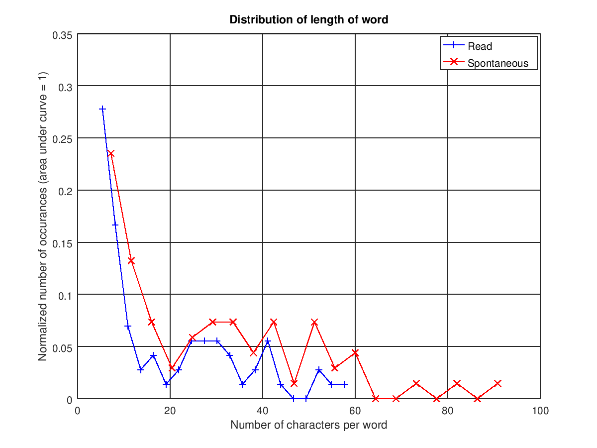
Figure 2: Word length (# of alphabets per word) for read and spontaneous speech.

2.3 Identifying Features

In the highly data-driven machine learning era, we opted to look for simple, yet effective features that could help in our pursuit. We considered a short technical passage consisting of two sentences and $62$ words, which we picked from Wikipedia for our analysis and asked (a) the paragraph to be read as is (read speech) and (b) the paragraph to be held as a reference and spoken in their own words ($\equiv$ spontaneous). We recorded this on a laptop as a $16$ kHz, $16$ bit, mono in .wav format. This read and spontaneous audio was processed by ds$()$ to produce a string of alphabets ($\in{\cal A}$). Fig. 2 shows a histogram plot of the number of alphabets in a word and their normalized frequency (area under the curve is $1$). It can be clearly observed that, (a) there are more words (with same number of alphabets) in spontaneously spoken passage compared to the read passage (the plot corresponding to spontaneous speech, in red is always above the read speech) and (b) there are more lengthy words in spontaneous speech (the spontaneous speech plot spreads beyond the read speech blue curve), there are words of length $90$ alphabets in spontaneous speech compared to $<60$ alphabets per word in read speech. This is in line with the observation that there are more ${\tt InActive}$ alphabets in spontaneous speech.

We extracted a set of $5$ meaningful features as mentioned in Table 1 for both the read and spontaneous speech. Note that these measured features are self explanatory and so we do not describe them in detail. Clearly, there are $3$ features (the duration (a), the number of alphabets (c), and the number of ${\tt Active}$ alphabets (d)) that show promise to discriminate read and the spontaneous speech.

Measured Values
SNo	What	Spontaneous	Read
(a)	Duration (sec)	47.62	29.67
(b)	Number of Words (#)	69	72
(c)	Number of Alphabets (#)	2382	1484
(d)	Number of ${\tt Active}$ alphabets (#)	1915	951
(e)	Number of ${\tt InActive}$ alphabets (#)	364	413
Derived Features
Ratio	What	Spontaneous	Read
${(c)}/{(b)}$	Av word len (alphabets/word; awl)	34.52	20.61
${(c)}/{(a)}$	Speaking Rate (alphabets/sec; aps)	50.02	50.02
${(b)}/{(a)}$	Word Rate (wps) $[f_{3}]$	1.45	2.43
${(e)}/{(a)}$	${\tt InActive}$ aps $[f_{2}]$	7.63	13.92
${(d)}/{(b)}$	${\tt Active}$ awl $[f_{1}]$	27.75	13.21

Table 1: Measured features from read and spontaneous speech for the same paragraph. # denotes is the count, an integer.

Based on the differences between read and spontaneous speech mentioned in [15] we derive (see Table 1 Derived Features) features like average word length (awl), speaking rate, word rate, ${\tt InActive}$ aps and ${\tt Active}$ awl, from the values directly measured from $\mbox{{\sc ds}}(x(t))$. It can be observed that, while ${\tt Active}$ average word length (${\tt Active}$ awl) and ${\tt InActive}$ alphabets per sec (${\tt InActive}$ aps) features show promise to be able to discriminate read and spontaneous speech, the speaking rate in terms of alphabets per sec (aps) is a feature that does not allow us to discriminate between read and spontaneous speech, this is to be expected because as we mentioned earlier, the total number of alphabets output by ds$()$ is proportional to the duration of the utterance. Clearly, the ${\tt Active}$ and ${\tt InActive}$ alphabets play an important role in discriminating read and spontaneous speech. As one would expect, there are a large number of $\diamond$ (can be associated with pauses) in spontaneous speech compared to read speech. Fig. 3 shows the plot of the ratio of number of ${\tt InActive}$ alphabets to the number of alphabets in a word (arranged in the increasing order). It can be observed that spontaneous speech has more ${\tt InActive}$ alphabets per word compared to the read speech. Note that the curve corresponding to spontaneous speech, in red, is always higher than the read speech (blue curve). This is expected, considering that there is a sizable amount of pause time in spontaneous speech, unlike read speech. We can further observe that the means value of the ratio (number of ${\tt InActive}$ alphabets to the number of alphabets) is higher for spontaneous speech ($0.76$) compared to read speech ($0.64$) as seen in Fig. 3.

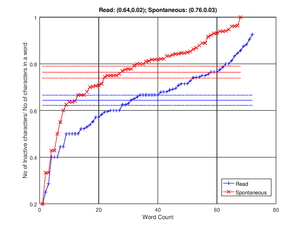
Figure 3: Ratio of # ${\tt InActive}$ alphabets to the # of alphabets in a word (arranged in the increasing order of ratio).

2.4 Proposed Classifier

As observed in the previous section, there exist features extracted from ${\tt DeepSpeech}$ that are able to discriminate read and spontaneous speech. However, the measured features (Table 1 (a), (c), (d)) though able to discriminate read and spontaneous speech are not useful because it requires a priori knowledge of the passage or information spoken by the speaker. On the other hand, there are a set of derived features, which are ratios and hence independent of the spoken passage. As seen in Table 1 some of these features are able to strongly discriminate read and spontaneous speech. The three derived features that show promise to discriminate read and spontaneous speech are

1. [$f_{1}$] ${\tt Active}$ awl

   (${\tt Active}$ alphabets per word is higher for spontaneous speech)

2. [$f_{2}$] ${\tt InActive}$ aps

   (${\tt InActive}$ alphabets per sec is lower for spontaneous speech)

3. [$f_{3}$] wps

   (Word Rate or Words per sec is lower for spontaneous speech)

Note that these features are independent of the duration of the audio utterance and they do not depend on what was spoken and entirely rely on how the utterance was spoken. This is important because any feature based on what was spoken would have a direct dependency on the performance accuracy of the speech-to-alphabet engine, in our case ${\tt DeepSpeech}$. In that sense our approach does not depend explicitly on the performance of the ${\tt DeepSpeech}$ and does not depend on the linguistic content of the spoken passage. The process of classifying a given utterance $u(t)$ is simple. We extract the features $f_{1},f_{2},f_{3}$ from the $\mbox{{\sc ds}}(x(t))$ for a given spoken passage $x(t)$ and compute a read score ${\cal R}$ using (2). We use (3) to determine if $x(t)$ is read speech or spontaneous speech.

$${\cal R}=\frac{1}{1+exp^{-\lambda_{1}(f_{1}-\tau_{1})}}+\frac{1}{1+exp^{\lambda_{2}(f_{2}-\tau_{2})}}+\frac{1}{1+exp^{-\lambda_{3}(f_{3}-\tau_{3})}}$$ (2)

$$x(t) = \mbox{Read Speech}\;\;\mbox{if}\;\;{\cal R}\geq\tau_{{\cal R}}$$ (3)

$$= \mbox{Spontaneous Speech}\;\;\mbox{if}\;\;{\cal R}<\tau_{{\cal R}}$$

We empirically chose $\lambda_{1,2,3}=1$, $\tau_{1}=6$, $\tau_{2}=10$, and $\tau_{3}=1.75$ based on observations made in Table 1. And $\tau_{{\cal R}}=1.75$, which is in the range ${\cal R}\in[0,3]$.

3 Experimental Validation

The selection of the features to discriminate between spontaneous and read speech is based on an intuitive understanding of the difference between read and spontaneous speech as mentioned in [15] and verified through observation of actual audio data (Table 1).

We collected audio data ($150$ minutes; spread over $7$ different programs) broadcast by All India Radio [13] called air-db which is available at [9]. This audio data is the recording between a host and a guest and consists of both spontaneous speech (guest) and read speech (host). We used a pre-trained speaker diarization model [8, 4] to segment the audio, which resulted in $1028$ audio segments. We discarded all audio segments below $2$ sec so that there was sizable amount of spoken information in any given audio segment; this resulted in a total of $657$ audio segments. All experimental results are reported on this $657$ audio segments (see Fig. 4).

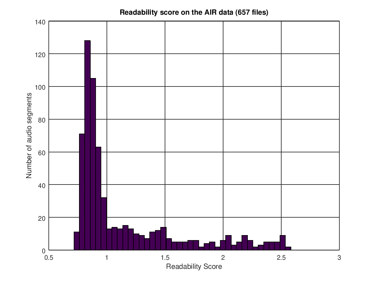
(a) Histogram of ${\cal R}$ score.

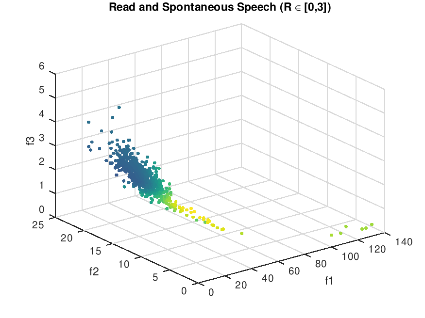
(b) ${\cal R}$ as a function of $f_{1},f_{2},f_{3}$.

Figure 4: Readability score (${\cal R}$) for $657$ audio segments ($>2$ sec) from air-db.

For each of these $657$ audio segments, $f_{1},f_{2},f_{3}$ were computed and then using (2) ${\cal R}$ was computed. Fig. 4(a) shows the distribution of the readability score ${\cal R}$ of the audio segments. Clearly a large number of audio segments ($535$) were classified as spontaneous speech compared to $122$, which was classified as read. Figure 4(b) shows the scatter plot of ${\cal R}$ for the $657$ audio segments as a function of $f_{1},f_{2},f_{3}$. The colour of the scatter plot represents the value of ${\cal R}$. Figure 5 shows the classification of segmented audio into read speech (violet; ${\cal R}\geq\tau_{\cal R}$) and spontaneous speech (yellow; ${\cal R}<\tau_{\cal R}$).

We choose $\delta=0.05$ and selectively listen to some of the audio segments (${\cal R}>(\tau_{\cal R}+\delta)$ and ${\cal R}<(\tau_{\cal R}-\delta)$) and found that almost all of the audio segments classified as spontaneous belong to the guest speaker (which is expected), however, several instances of host speech was also classified as spontaneous.

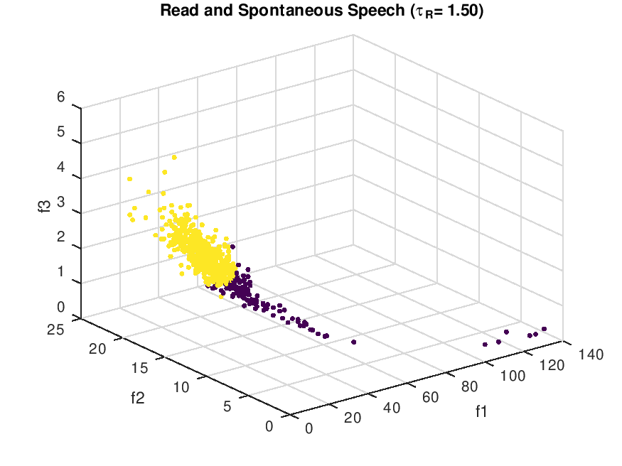
Figure 5: $657$ audio segments from air-db classified as read speech (violet) and spontaneous speech (yellow).

We hypothesize, that radio hosts are trained to speak even written text to give a feeling of spontaneity to the listener. We then looked at the $23$ audio segments which had ${\cal R}$ in the range $[\tau_{\cal R}-\delta,\tau_{\cal R}+\delta]$ and hence in the neighbourhood of $\tau_{\cal R}$ which is more prone to classification errors. We observed that there were $12$ and $11$ read speech and spontaneous speech segments respectively. Of the $12$ audio segments classified as read speech, $4$ audio segments were actually spontaneous while of the $11$ audio segments classified as spontaneous speech, $3$ audio segments were actually read speech (see Table 2). It should be noted that, in the neighbourhood of the $\tau_{\cal R}$, where the confusion is expected to be very high, the proposed classifier is able to correctly classify with an accuracy of $\approx 70\%$ ($16$ of the $23$ audio segments correctly classified).

${\cal R}\in$	Ground Truth
$[\tau_{\cal R}-\delta,\tau_{\cal R}+\delta]$	Read Speech	Spont
Read Speech	8	4
Spontaneous	3	8

Table 2: Performance on $23$ audio segments whose ${\cal R}\in[\tau_{\cal R}-\delta,\tau_{\cal R}+\delta]$. $4$ spontaneous speech audio segments were classified as read speech and $3$ read speech segments were classified as spontaneous speech.

Very recently, we came across the Archive of L1 and L2 Scripted and Spontaneous Transcripts And Recordings (allsstar-db) corpus [3]. We picked up speech data corresponding to $26$ English speakers ($14$ Female and $12$ Male). Each speaker spoke a maximum of $8$ utterances ($4$ spontaneous and $4$ read) in different settings. The $4$ read speech were (a) DHR ($20$ formal sentences picked from the Universal Declaration of Human Rights; average duration $106.2$ s) , (b) HT2 (simple sentences; phonetically balanced which was created for Hearing in Noise Test; average duration $100.5$ s), (c) LPP ($33$ sentences picked from Le Petit Prince, average duartion $107.1$ s) and (d) NWS (North Wind and the Sun Passage, average duration $32.8$ s); while the $4$ spontaneous speech utterances were (a) QNA (Spontaneous speech about anything for $5$ minutes; average duration $317.5$ s), (b) ST2 (wordless pictures from "Bubble Bubble" used to elicit spontaneous speech; average duration $88.8$ s), (c) ST3 (wordless pictures from "Just a Pig at Heart"; average duration $78.2$ s), and (d) ST4 (wordless pictures from "Bear’s New Clothes"; average duration $85.2$ s).

Gen	SpkID	R (DHR, HT2, LPP, NWS)	S (QNA, ST2, ST3, ST4)	(minutes)
F	49	4 (1, 1, 1, 1)	4 (1, 1, 1, 1)	8 (13.47)
	51	4 (1, 1, 1, 1)	4 (1, 1, 1, 1)	8 (16.87)
	56	4 (1, 1, 1, 1)	4 (1, 1, 1, 1)	8 (19.29)
	58	4 (1, 1, 1, 1)	4 (1, 1, 1, 1)	8 (16.73)
	60	4 (1, 1, 1, 1)	4 (1, 1, 1, 1)	8 (12.32)
	62	4 (1, 1, 1, 1)	4 (1, 1, 1, 1)	8 (12.78)
	63	4 (1, 1, 1, 1)	4 (1, 1, 1, 1)	8 (19.42)
	64	4 (1, 1, 1, 1)	4 (1, 1, 1, 1)	8 (16.06)
	65	4 (1, 1, 1, 1)	4 (1, 1, 1, 1)	8 (12.70)
	67	4 (1, 1, 1, 1)	4 (1, 1, 1, 1)	8 (15.04)
	68	4 (1, 1, 1, 1)	4 (1, 1, 1, 1)	8 (12.91)
	69	4 (1, 1, 1, 1)	4 (1, 1, 1, 1)	8 (14.90)
	71	4 (1, 1, 1, 1)	4 (1, 1, 1, 1)	8 (12.87)
	72	4 (1, 1, 1, 1)	4 (1, 1, 1, 1)	8 (15.67)
M	50	4 (1, 1, 1, 1)	4 (1, 1, 1, 1)	8 (14.28)
	52	4 (1, 1, 1, 1)	4 (1, 1, 1, 1)	8 (25.4)
	53	4 (1, 1, 1, 1)	4 (1, 1, 1, 1)	8 (13.27)
	55	4 (1, 1, 1, 1)	4 (1, 1, 1, 1)	8 (13.27)
	57	4 (1, 1, 1, 1)	4 (1, 1, 1, 1)	8 (19.26)
	59	4 (1, 1, 1, 1)	4 (1, 1, 1, 1)	8 (13.60)
	61	4 (1, 1, 1, 1)	4 (1, 1, 1, 1)	8 (14.37)
	66	4 (1, 1, 1, 1)	4 (1, 1, 1, 1)	8 (14.67)
	70	4 (1, 1, 1, 1)	4 (1, 1, 1, 1)	8 (12.97)
	131	4 (1, 1, 1, 1)	2 (1, 1, 0, 0)	6 (11.89)
	132	4 (1, 1, 1, 1)	2 (1, 1, 0, 0)	6 (12.19)
	133	4 (1, 1, 1, 1)	2 (1, 1, 0, 0)	6 (12.64)
Total	26 (Speakers)	104 (26, 26, 26, 26)	98 (26, 26, 23, 23)	202 (388.9)

Table 3: allsstar-db corpus details.

In all there were $202$ audio utterances of which $104$ were read utterances and $98$ were spontaneous spoken utterances. Note that in all there should have been $104$ spontaneous utterances; but $2$ spontaneous utterances each were missing from $3$ male participants. Table 3 shows the distribution of data from allsstar-db. Experiments were carried out on these $202$ audio utterances from $26$ people. We went through the process of passing through audio utterance through the ${\tt DeepSpeech}$, followed by extraction of three features and computing of ${\cal R}$ as mentioned in (2). The experimental results are shown as a confusion matrix in Table 4. As can be observed, the performance of our proposed scheme is $88.12\%$. Figure 6 shows the utterances in the feature space $(f_{1},f_{2},f_{3})$ for allsstar-db. The classification based on the approach mentioned earlier in this paper is shown in Fig. 6 (a) the utterances classified as read and spontaneous have been marked in yellow and violet respectively. Figure 6 (b) captures the utterances which have been correctly recognised (represented in green). The read utterances mis-recognized as spontaneous is shown in red ($8$ utterances) while the utterances corresponding to spontaneous speech which have been recognized as read have been represented in purple ($16$ utterances).

	Ground Truth
	Read	Spontaneous
Read	88 (84.62%)	8
Spontaneous	16	90 (91.84%)

Table 4: Confusion Matrix. Performance Accuracy on allsstar-db $88.12\%$.

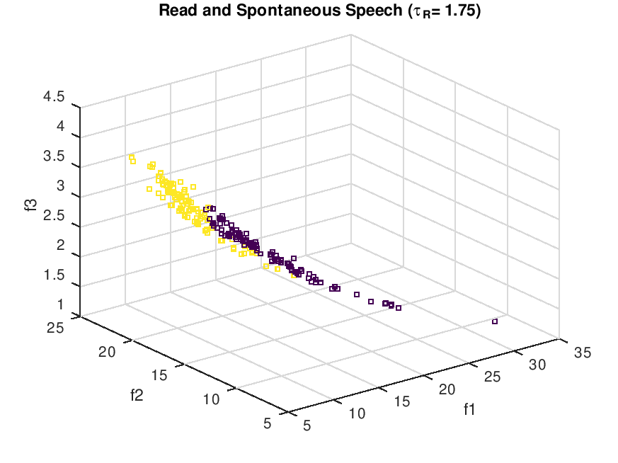
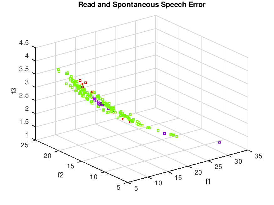
(a) (b)

Figure 6: Classification results on allsstar-db. (a) Yellow represents read speech while violet corresponds to spontaneous speech and (b) Green shows the correctly recognized utterances (88.12%) while red represents read speech recognized as spontaneous and purple shows the utterances corresponding to spontaneous speech which have been recognized as read.

We analyzed further to understand the mis-recognized utterances. The spontaneous utterances of speakers with ID $49,56,58,60,71(2),57,$ and $59$ were mis-recognized as read speech while read utterances with speakers ID $56,58(2),64(3),$ $69,71(2),50(2),52,55,66(2),133$ were recognized as being spontaneous. As shown in Table 5 we observe that majority of the speakers were mis-recognized either as reading while they had spoken spontaneously (column 1) or as being spontaneous when they had actually read (column 2). Only speakers with SpkID $56,58$ and $71$ (column 3) were mis-recognized both ways, namely their read speech was recognized as spontaneous and vice-versa.

	Spontaneous $\rightarrow$ Read	Read $\rightarrow$ Spontaneous	Read $\leftrightarrow$ Spontaneous
Female	$49(1),60(1)$	$64(3),69(1)$	$56(2),58(3),71(4)$
Male	$57(1),59(1)$	$50(2),52(1),55(1),66(2),133(1)$	-

Table 5: Mis-recognition based on Speaker ID. The number in parenthesis shows the number of instances.

We observe that the speaker with ID $71$ had ${\cal R}\in[1.63,1.82]$; we carefully listened to all the utterances and found very less perceptual difference between read and spontaneous utterances. While the read utterances of the speaker with ID $66$ had large silences between sentences (an indication of spontaneous speech) which lead to almost all of the read utterances being recognized as spontaneous.

4 Conclusion

In this paper, we proposed a simple classifier to identify read and spontaneous speech. The novelty of the classifier is in deriving a very small set of features, indirectly from the audio segment. Most of the literature which directly or indirectly address recognition of spontaneous speech have done by analyzing audio signal for determining speech specific properties like intonation, repetition of words, filler words, etc. We derived a small set of explainable features from a string of alphabets derived from the output of the ${\tt DeepSpeech}$ speech-to-alphabet recognition engine. The features are self explanatory and capture the essential difference between read and spontaneous speech as mentioned in [15]. The derived features are based on how the utterance was spoken and not on what was spoken thereby making the features independent of the linguistic content of the utterance. Experiments conducted on our own data-set (air-db) and publicly available allsstar-db shows the classifier to perform very well. The main advantage of the proposed scheme is that the features are explainable and are derived by processing the alphabet string output of $\mbox{{\sc ds}}()$. It should be noted that while we can categorize our approach as being devoid of deep model training or learning; the dependency on ${\tt DeepSpeech}$ pre-trained deep architecture model (as a black-box) cannot be ignored.

References

- [1] Asami, T., Masumura, R., Masataki, H., Sakauchi, S.: Read and spontaneous speech classification based on variance of GMM supervectors. In: Fifteenth Annual Conference of the International Speech Communication Association (2014)
- [2] Batliner, A., Kompe, R., Kießling, A., Nöth, E., Niemann, H.: Can you tell apart spontaneous and read speech if you just look at prosody? In: Speech Recognition and Coding, pp. 321–324. Springer (1995)
- [3] Bradlow, A.R.: ALLSSTAR: archive of L1 and L2 scripted and spontaneous transcripts and recordings. https://speechbox.linguistics.northwestern.edu/ (2023)
- [4] Bredin, H., Yin, R., Coria, J.M., Gelly, G., Korshunov, P., Lavechin, M., Fustes, D., Titeux, H., Bouaziz, W., Gill, M.P.: pyannote.audio: neural building blocks for speaker diarization. In: ICASSP 2020, IEEE International Conference on Acoustics, Speech, and Signal Processing. Barcelona, Spain (May 2020)
- [5] Dellwo, V., Leemann, A., Kolly, M.J.: The recognition of read and spontaneous speech in local vernacular: The case of zurich german. Journal of Phonetics 48, 13–28 (2015). https://doi.org/https://doi.org/10.1016/j.wocn.2014.10.011, https://www.sciencedirect.com/science/article/pii/S009544701400093X, the Impact of Stylistic Diversity on Phonetic and Phonological Evidence and Modeling
- [6] Dufour, R., Estève, Y., Deléglise, P.: Characterizing and detecting spontaneous speech: Application to speaker role recognition. Speech Commun. 56, 1–18 (2014)
- [7] Eren, O., Kılıç, M., Bada, E.: Fluency in l2: Read and spontaneous speech pausing patterns of turkish, swahili, hausa and arabic speakers of english. Journal of Psycholinguistic Research pp. 1–17 (2021)
- [8] Huggingface: speaker-diarization. https://huggingface.co/pyannote/speaker-diarization (pyannote/speaker-diarization@2022072, 2022)
- [9] Kopparapu, S.K.: Air-DB: A dataset for classifying spontaneous and read speech. https://drive.google.com/drive/folders/1-31cSrppLGiG1bgij6rFlnw5rChifi5C?usp=sharing (2022)
- [10] Mozilla: Deepspeech. https://github. com/mozilla/DeepSpeech/releases (Jan 2019)
- [11] Mukherji, K., Pandharipande, M., Kopparapu, S.K.: Improved language models for asr using written language text. In: 2022 National Conference on Communications (NCC). pp. 362–366 (2022). https://doi.org/10.1109/NCC55593.2022.9806803
- [12] Panayotov, V., Chen, G., Povey, D., Khudanpur, S.: Librispeech: an asr corpus based on public domain audio books. In: 2015 IEEE International Conference on Acoustics, Speech and Signal Processing (ICASSP). pp. 5206–5210. IEEE (2015)
- [13] PrasarBharati: All India Radio. https://newsonair.gov.in/ (2022)
- [14] Tripathi, A., Bhosale, S., Kopparapu, S.K.: Automatic speaker independent dysarthric speech intelligibility assessment system. Computer Speech & Language 69, 101213 (2021). https://doi.org/https://doi.org/10.1016/j.csl.2021.101213, https://www.sciencedirect.com/science/article/pii/S0885230821000206
- [15] Ward, W.: Understanding spontaneous speech. Speech and Natural Language Workshop pp. 365–367 (1989)