PrivaScissors: Enhance the Privacy of Collaborative Inference through the Lens of Mutual Information

Abstract

Edge-cloud collaborative inference empowers resource-limited IoT devices to support deep learning applications without disclosing their raw data to the cloud server, thus preserving privacy. Nevertheless, prior research has shown that collaborative inference still results in the exposure of data and predictions from edge devices. To enhance the privacy of collaborative inference, we introduce a defense strategy called PrivaScissors, which is designed to reduce the mutual information between a model’s intermediate outcomes and the device’s data and predictions. We evaluate PrivaScissors’s performance on several datasets in the context of diverse attacks and offer a theoretical robustness guarantee.

1 Introduction

Edge devices are rapidly evolving, becoming smarter and more versatile. These devices are expected to perform a wide range of deep learning (DL) inference tasks with high efficiency and remarkable performance. However, implementing DL inference applications on such edge devices can be quite challenging due to the constraints imposed by the on-device resource availability. As we see the rise of state-of-the-art DL models, such as Large Language Models, they are becoming increasingly complex, housing a colossal number of parameters. This escalation in complexity and size makes it difficult to store a DL model on an edge device, which typically has limited memory space. Furthermore, the restricted computational resources could lead to unacceptably long latency during inference. One potential solution to this predicament is to transmit the input data directly from the edge device to a cloud server. The server, which houses the DL model, then conducts inference and sends the prediction back to the device. However, this approach carries with it the risk of privacy breaches, particularly if the input data are sensitive in nature - such as facial images. It’s also important to note that the predictions can also contain confidential information, such as the patient’s diagnostic results.

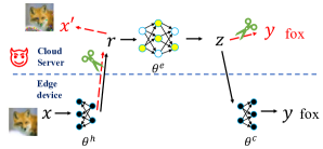
Figure 1: A general framework of collaborative inference. The malicious server can infer data and predictions on the edge device. PrivaScissors defends against privacy leakage by reducing the mutual information between the model’s intermediate outcomes and the edge device’s data and predictions.

Collaborative inference [1, 2, 3] has become a privacy-preserving approach to deploying DL inference applications on commodity edge devices that have limited computing resources. Fig. 1 shows a general collaborative inference system. Suppose an edge device and a cloud server conduct collaborative inference. The deep learning model can be divided into three parts. The first and last few layers of the network are deployed on the edge device, while the remaining layers are offloaded to a cloud server. This division allows most of the computational tasks to be handled by the server, effectively mitigating the resource limitations on the device. The edge device and the cloud server communicate only the intermediate outputs of the model, ensuring that the raw data and predictions remain inaccessible to the server. However, recent works [4, 5] have revealed that sharing these intermediate outputs can still lead to data and prediction leakage. A malicious server can, for instance, reconstruct input data from the representations (i.e., $r$ in Fig. 1) uploaded by the device through Model Inversion (MI) attacks [6, 7, 5]. Furthermore, the high-level features (i.e., $z$ in Fig. 1) contain rich information about the predictions, making it feasible for a malicious server to infer the device’s predictions through these features [8, 9, 10]. While there have been considerable explorations into privacy preservation in collaborative inference [4, 5, 11, 12], existing defenses tend to significantly degrade model utility. This degradation is particularly evident in scenarios where attacks are relatively strong. For example, when the head model on the device (i.e., $\theta^{h}$ in Fig. 1) is shallow, existing defenses cannot guarantee the privacy of the input data without a significant drop in model accuracy.

We propose a defense method named PrivaScissors, designed from a mutual information perspective to enhance the edge device’s privacy in collaborative inference. This approach works by protecting both the device’s data and its predictions. To protect the device’s data, we regularize the head model on the device to extract representations that hold less mutual information with the input. To protect the prediction, we regularize the features extracted by the server’s encoder to minimize the mutual information they contain with the label. We derive a variational mutual information upper-bound and develop an adversarial training method to minimize this bound on the device side. Our defense’s robustness is theoretically guaranteed. We evaluate PrivaScissors on CIFAR10 and CIFAR100 against both black-box and white-box MI attacks. The results show that PrivaScissors can effectively defend the attacks with less than a 3% drop in model accuracy even when the head model on the device has only one convolutional layer, where the attacks are extremely strong. We also evaluate our defense against prediction leakage using multiple model completion (MC) attacks [8, 9]. The results show that our defense achieves the best trade-off between the model accuracy and defending effectiveness compared with the baselines.

Our contributions are summarized as follows:

• To the best of our knowledge, this is the first paper to systematically address the privacy leakage in collaborative inference, encompassing both data leakage and prediction leakage.

• We propose a defense method against data and prediction leakage in collaborative inference from the mutual information perspective. We offer a theoretical robustness guarantee of our defense against general privacy leakage from the intermediate outcomes of a model.

• We empirically evaluate our defense across multiple datasets and against multiple attacks. The results show that our defense can defend MI attacks while preserving high accuracy, even when the head model has only one convolutional layer. Our defense can also prevent prediction leakage against MC attacks with nearly no model accuracy drop.

2 Related Work

2.1 Privacy Leakage in Collaborative Inference

Privacy leakage is drawing more and more attention as the rapid growth of commercial deployment of deep learning, especially in collaborative learning scenarios, whose primary concern is privacy. In collaborative inference, we categorize privacy leakage into two types, i.e., data leakage [13, 4, 14, 15] and prediction leakage [8, 9, 10].

For data leakage, [13] proposes general attack methods for complex models, such as Neural Networks, by matching the correlation between adversary features and target features, which can be seen as a variant of model inversion [16, 17]. [4, 18, 15, 19, 20, 14] also propose variants of model inversion attack. While all these attacks are in the inference phase, [15] proposes a variant of DLG [6] which can perform attacks in the training phase. For prediction leakage, [9] proposes an attack and defense method for two-party split learning on binary classification problems, a special collaborative inference setting. Additionally, [8] proposes three different label inference attack methods considering different settings in collaborative inference: direct label inference attack, passive label inference attack, and active label inference attack.

2.2 Defense in Collaborative Inference

Defensive methods have also been proposed against privacy leakage in collaborative inference. To defend against data leakage, some works apply differential privacy (DP) [4, 5] and compression [4, 5, 11] to the representations and models. These methods can sometimes defend against data leakage from the representation, but they also cause substantial model performance degradation because they destroy the knowledge/information in the representations. Two recent works also try to solve the data leakage problem from the mutual information perspective [11, 12]. However, their methods only achieve decent results when the head model on the edge device is deep, which is not practical when the computation power is constrained on the edge device. To defend against prediction leakage, [10] manipulates the labels following specific rules to defend the direct label inference attack, which can be seen as a variant of label differential privacy (label DP) [21, 22] in collaborative inference. Compression and quantization of the gradients [8, 12] are also applied to defend against prediction leakage. However, similarly to the defense against data leakage, these defenses cause substantial model performance degradation to achieve decent defending performance.

3 Preliminary

3.1 Collaborative Inference Setting

Suppose an edge device and a cloud server conduct collaborative inference. Following the setting in Fig. 1, the deep learning model is divided into a head model $f^{h}_{\theta^{h}}$, an encoder $f^{e}_{\theta^{e}}$ and a classifier $f^{c}_{\theta^{c}}$. The head model and classifier are deployed on the edge device, and the encoder is on the cloud server. Given an input $x_{i}$, the edge device first calculates the representation $r_{i}=f^{h}_{\theta^{h}}(x_{i})$ and sends $r_{i}$ to the server. Then the server extracts the feature from the received representation $z_{i}=f^{e}_{\theta^{e}}(r_{i})$ and sends the feature back to the edge device. After receiving the feature, the edge device calculates the prediction $\hat{y}_{i}=f^{c}_{\theta^{c}}(z_{i})$. In this paper, the results of $f^{h}_{\theta^{h}}$ sent from the device to the server are referred to as representations, and features refer to the results of $f^{e}_{\theta^{e}}$ sent from the server to the device. The overall inference procedure can be formulated as

$$\hat{y}_{i}=f^{c}_{\theta^{c}}(f^{e}_{\theta^{e}}(f^{h}_{\theta^{h}}(x_{i}))).$$ (1)

In the real world, the raw data $x_{i}$ and prediction $\hat{y}_{i}$ are important intelligent properties of the edge device and may contain private information. In the inference procedure, the edge device does not send raw data to the server, and the inference results are also inaccessible to the server.

3.2 Threat Model

We consider that the edge device possessing the head model and the classifier is trusted. The edge device only uploads the representations to the server and never leaks raw data or predictions to the server. However, the cloud server is untrusted, attempting to steal raw data and predictions. We assume the untrusted server strictly follows the collaborative inference protocols, and it cannot compromise the inference process conducted by the edge device. With the received representation $r_{i}$, the server can reconstruct the input data $x_{i}$ on the edge device by conducting model inversion (MI) attacks [6, 7, 4]. Notably, the head model on the edge device is usually shallow due to the computation resource limitation, which aggravates data leakage vulnerability from the representation [5]. The encoder on the server extracts high-level features containing rich information about the prediction, which enables the server to infer predictions of the device.

4 Method

4.1 Defense Formulation

To defend against privacy leakage, we propose a learning algorithm that regularizes the model during the training phase. Following the setup of 3.1, suppose the edge device has sample pairs $\left\{\left(x_{i},y_{i}\right)\right\}_{i=1}^{N}$ drawn from a distribution $p\left({\textnormal{x}},{\textnormal{y}}\right)$. The representation is calculated as ${\textnormal{r}}=f^{h}_{\theta^{h}}({\textnormal{x}})$ by the edge device, and the cloud server computes features ${\textnormal{z}}=f^{e}_{\theta^{e}}({\textnormal{r}})$. We apply ${\textnormal{x}},{\textnormal{y}},{\textnormal{r}},{\textnormal{z}}$ here to represent random variables, while $x_{i},y_{i},r_{i},z_{i}$ are deterministic values. To preserve the privacy of the edge device’s raw data and inference results, our learning algorithm is to achieve three goals:

• Goal 1: To preserve the performance of collaborative inference, the main objective loss should be minimized.

• Goal 2: To reduce the data leakage from the representations, $\theta^{h}$ should not extract representations r containing much information about the raw data x.

• Goal 3: To reduce the leakage of the predictions on the edge device, $\theta^{e}$ on the cloud server should not be able to extract features z containing much information about the true label y.

Formally, we have three training objectives:

$$\textbf{Prediction:}\min\limits_{\theta^{h},\theta^{e},\theta^{c}}\mathcal{L}\left(f^{c}_{\theta^{c}}\left(f^{e}_{\theta^{e}}\left(f^{h}_{\theta^{h}}({\textnormal{x}})\right)\right),{\textnormal{y}}\right),$$ (2)

$$\textbf{Data protection:}\min\limits_{\theta^{h}}\text{I}({\textnormal{r}};{\textnormal{x}}),$$

$$\textbf{Prediction protection:}\min\limits_{\theta^{h},\theta^{e}}\text{I}({\textnormal{z}};{\textnormal{y}}),$$

where $\text{I}({\textnormal{r}};{\textnormal{x}})$ is the mutual information between the representation and the data, which indicates how much information r preserves for the data x. Similarly, $\text{I}({\textnormal{z}};{\textnormal{y}})$ is the mutual information between the feature and the label. We minimize these mutual information terms to prevent the cloud server from inferring the data x and label y from r and z, respectively.

The prediction objective is usually easy to optimize (e.g., cross-entropy loss for classification). However, the mutual information terms are hard to calculate in practice for two reasons: 1. r and x are high-dimensional, and it is extremely computationally heavy to compute their joint distribution; 2. Calculating the mutual information requires knowing the distributions p(x|r) and p(y|z), which are both difficult to compute. To derive tractable estimations of the mutual information objectives, we leverage CLUB[23] to formulate variational upper-bounds of mutual information terms. We first formulate a variational upper-bound of $\text{I}({\textnormal{r}};{\textnormal{x}})$:

$$\text{I}\left({\textnormal{r}};{\textnormal{x}}\right)$$ (3)

$$\leq{} \text{I}_{\text{{vCLUB}}}\left({\textnormal{r}};{\textnormal{x}}\right)$$

$$:={} \mathbb{E}_{p\left({\textnormal{r}},{\textnormal{x}}\right)}\log q_{\psi}\left({\textnormal{x}}|{\textnormal{r}}\right)-\mathbb{E}_{p\left({\textnormal{r}}\right)p\left({\textnormal{x}}\right)}\log q_{\psi}\left({\textnormal{x}}|{\textnormal{r}}\right),$$

where $q_{\psi}\left({\textnormal{x}}|{\textnormal{r}}\right)$ is a variational distribution with parameters $\psi$ to approximate $p\left({\textnormal{x}}|{\textnormal{r}}\right)$. To guarantee the inequality of Eq. 3, $q_{\psi}\left({\textnormal{x}}|{\textnormal{r}}\right)$ should satisfy

$$\text{KL}\left(p\left({\textnormal{r}},{\textnormal{x}}\right)||q_{\psi}\left({\textnormal{r}},{\textnormal{x}}\right)\right)\leq\text{KL}\left(p\left({\textnormal{r}}\right)p\left({\textnormal{x}}\right)||q_{\psi}\left({\textnormal{r}},{\textnormal{x}}\right)\right),$$ (4)

which can be achieved by minimizing $\text{KL}\left(p\left({\textnormal{r}},{\textnormal{x}}\right)||q_{\psi}\left({\textnormal{r}},{\textnormal{x}}\right)\right)$:

$$\psi~{}={} \arg\min\limits_{\psi}\text{KL}\left(p\left({\textnormal{r}},{\textnormal{x}}\right)||q_{\psi}\left({\textnormal{r}},{\textnormal{x}}\right)\right)$$ (5)

$$={} \arg\min\limits_{\psi}\mathbb{E}_{p\left({\textnormal{r}},{\textnormal{x}}\right)}\left[\log\left(p\left({\textnormal{x}}|{\textnormal{r}}\right)p\left({\textnormal{r}}\right)\right)-\log\left(q_{\psi}\left({\textnormal{x}}|{\textnormal{r}}\right)p\left({\textnormal{r}}\right)\right)\right]$$

$$={} \arg\max\limits_{\psi}\mathbb{E}_{p\left({\textnormal{r}},{\textnormal{x}}\right)}\log\left(q_{\psi}\left({\textnormal{x}}|{\textnormal{r}}\right)\right).$$

With sample pairs $\left\{\left(x_{i},y_{i}\right)\right\}_{i=1}^{N}$, we can apply the sampled vCLUB (vCLUB-S) mutual information estimator in [23] to reduce the computational overhead, which is an unbiased estimator of $\text{I}_{\text{{vCLUB}}}$ and is formulated as

$$\hat{\text{I}}_{\text{vCLUB-S}}({\textnormal{r}};{\textnormal{x}})=\frac{1}{N}\sum\limits_{i=1}^{N}\left[\log q_{\psi}\left(x_{i}|r_{i}\right)-\log q_{\psi}\left(x_{k_{i}^{\prime}}|r_{i}\right)\right],$$ (6)

where $k_{i}^{\prime}$ is uniformly sampled from indices $\{1,...,N\}$. With Eq. 3, Eq. 5 and Eq. 6, the objective of data protection is formulated as:

$$\min\limits_{\theta^{h}}\text{I}({\textnormal{r}};{\textnormal{x}})\Leftrightarrow~{}\min\limits_{\theta^{h}}\hat{\text{I}}_{\text{vCLUB-S}}({\textnormal{r}};{\textnormal{x}})$$ (7)

$$={} \min\limits_{\theta^{h}}\frac{1}{N}\sum\limits_{i=1}^{N}\left[\max\limits_{\psi}\log q_{\psi}\left(x_{i}|r_{i}\right)-\log q_{\psi}\left(x_{k_{i}^{\prime}}|r_{i}\right)\right].$$

Similarly, we can use a variational distribution $q_{\phi}(y|z)$ with parameter $\phi$ to approximate $p(y|z)$, and formulate the objective of label protection as:

$$\min\limits_{\theta^{h},\theta^{e}}\text{I}({\textnormal{z}};{\textnormal{y}})\Leftrightarrow~{}\min\limits_{\theta^{h},\theta^{e}}\hat{\text{I}}_{\text{vCLUB-S}}({\textnormal{z}};{\textnormal{y}})$$ (8)

$$={} \min\limits_{\theta^{h},\theta^{e}}\frac{1}{N}\sum\limits_{i=1}^{N}\left[\max\limits_{\phi}\log q_{\phi}\left(y_{i}|z_{i}\right)-\log q_{\phi}\left(y_{n_{i}^{\prime}}|z_{i}\right)\right].$$

Suppose we use $g_{\psi}$, $h_{\phi}$ to parameterize $q_{\psi}$ and $q_{\phi}$, respectively. By combining Eq. 7, Eq. 8 and the prediction objective with weight hyper-parameters $\lambda_{d}$ and $\lambda_{l}$, we formulate the overall optimizing objective as

$$\min\limits_{\theta^{h},\theta^{e},\theta^{c}}(1-\lambda_{d}-\lambda_{l})\underbrace{\frac{1}{N}\sum\limits_{i=1}^{N}\mathcal{L}\left(f^{c}_{\theta^{c}}\left(f^{e}_{\theta^{e}}\left(f^{h}_{\theta^{h}}(x_{i})\right)\right),y_{i}\right)}_{\mathcal{L}_{c}}$$ (9)

$$+\min\limits_{\theta^{h}}\max\limits_{\psi}\lambda_{d}\underbrace{\frac{1}{N}\sum\limits_{i=1}^{N}\log g_{\psi}\left(x_{i}|f^{h}_{\theta^{h}}(x_{i})\right)}_{\mathcal{L}_{d\_a}}+\min\limits_{\theta^{h}}\lambda_{d}\underbrace{\frac{1}{N}\sum\limits_{i=1}^{N}-\log g_{\psi}\left(x_{k_{i}^{\prime}}|f^{h}_{\theta^{h}}(x_{i})\right)}_{\mathcal{L}_{d\_r}}$$

$$+\min\limits_{\theta^{h},\theta^{e}}\max\limits_{\phi}\lambda_{l}\underbrace{\frac{1}{N}\sum\limits_{i=1}^{N}\log h_{\phi}\left(y_{i}|f^{e}_{\theta^{e}}\left(f^{h}_{\theta^{h}}(x_{i})\right)\right)}_{\mathcal{L}_{l\_a}}+\min\limits_{\theta^{h},\theta^{e}}\lambda_{l}\underbrace{\frac{1}{N}\sum\limits_{i=1}^{N}-\log h_{\phi}\left(y_{n_{i}^{\prime}}|f^{e}_{\theta^{e}}\left(f^{h}_{\theta^{h}}(x_{i})\right)\right)}_{\mathcal{L}_{l\_r}}.$$

$h_{\phi}$ can be easily constructed to estimate $p\left({\textnormal{y}}|{\textnormal{z}}\right)$ given the task of inference (e.g., classifier for classification task). To estimate $p\left({\textnormal{x}}|{\textnormal{r}}\right)$, we assume that x follows the Gaussian distribution of which the mean vector is determined by r and the variance is 1. Under this assumption, we apply a generator $g_{\psi}$ to estimate the mean vector of x given r.

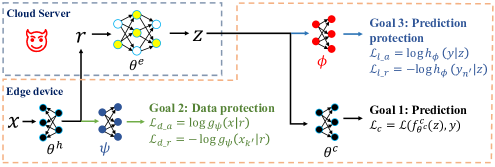
Figure 2: An overview of PrivaScissors. Training step 1: Optimize the classifiers $\theta^{c}$ and $\phi$ by minimizing $\mathcal{L}_{c}$ and maximizing $\mathcal{L}_{l\_a}$, respectively. Step 2: Optimize the generator $\psi$ by maximizing $\mathcal{L}_{d\_a}$. Step 3: Optimize $\theta^{h}$ and $\theta_{e}$ by minimizing $(1-\lambda_{d}-\lambda_{l})\mathcal{L}_{c}+\lambda_{l}\mathcal{L}_{l\_a}+\lambda_{l}\mathcal{L}_{l\_r}+\lambda_{d}\mathcal{L}_{d\_a}+\lambda_{d}\mathcal{L}_{d\_r}$.

4.2 Learning Algorithm

The overall objective has five terms. For simplicity, we denote these five objective terms as $\mathcal{L}_{c}$, $\mathcal{L}_{d\_a}$, $\mathcal{L}_{d\_r}$, $\mathcal{L}_{l\_a}$ and $\mathcal{L}_{l\_r}$, respectively, as shown in Eq. 9. $\mathcal{L}_{c}$ is the prediction objective. $\mathcal{L}_{d\_a}$ and $\mathcal{L}_{d\_r}$ comprise the data protection objective. $\mathcal{L}_{d\_a}$ is an adversarial training objective where an auxiliary generator $g_{\psi}$ is trained to capture data information while the head layers $f^{h}_{\theta^{h}}$ are trained to extract as little data information as possible. $\mathcal{L}_{d\_r}$ regularizes $f^{h}_{\theta^{h}}$ to extract representations that can be used to generate randomly picked samples. $\mathcal{L}_{l\_a}$ and $\mathcal{L}_{l\_r}$ have similar effect with $\mathcal{L}_{d\_a}$ and $\mathcal{L}_{d\_r}$, respectively. We can reorganize the overall training objective as

$$\theta^{h},\theta^{e},\theta^{c},\psi,\phi=~{}\arg\min\limits_{\theta^{h},\theta^{e}}\left[(1-\lambda_{d}-\lambda_{l})\min\limits_{\theta^{c}}\mathcal{L}_{c}+\lambda_{l}\max\limits_{\phi}\mathcal{L}_{l\_a}+\lambda_{l}\mathcal{L}_{l\_r}+\lambda_{d}\max\limits_{\psi}\mathcal{L}_{d\_a}+\lambda_{d}\mathcal{L}_{d\_r}\right].$$ (10)

Based on Eq. 10, we develop a collaborative learning algorithm. For each batch of data, the device first optimizes the classifiers $\theta^{c}$ and $\phi$ by minimizing $\mathcal{L}_{c}$ and maximizing $\mathcal{L}_{l\_a}$, respectively. Then, the device optimizes the generator $\psi$ by maximizing $\mathcal{L}_{d\_a}$. Finally, $\theta^{h}$ and $\theta_{e}$ are optimized by minimizing $(1-\lambda_{d}-\lambda_{l})\mathcal{L}_{c}+\lambda_{l}\mathcal{L}_{l\_a}+\lambda_{l}\mathcal{L}_{l\_r}+\lambda_{d}\mathcal{L}_{d\_a}+\lambda_{d}\mathcal{L}_{d\_r}$. The detailed algorithm can be found in Appendix A. Note that $\theta^{h},\theta^{c},\psi$ and $\phi$ are deployed on devices, and their training does not need additional information from the cloud server compared with training without our defense. The training procedure of $\theta^{e}$ does not change, which makes our defense concealed from the cloud server.

4.3 Robustness Guarantee

We derive certified robustness guarantees for our defenses against prediction and data leakage. Following the notations in Sec. 4.1, we have the following theorem of robustness guarantee for prediction leakage after applying PrivaScissors. All the proofs can be found in Appendix B.

Theorem 1

Let $h_{\phi}$ parameterize $q_{\phi}$ in Eq. 8. Suppose the malicious server optimizes an auxiliary model $h^{m}({\textnormal{y}}|{\textnormal{z}})$ to estimate $p({\textnormal{y}}|{\textnormal{z}})$. For any $h^{m}({\textnormal{y}}|{\textnormal{z}})$, we always have:

$$\frac{1}{N}\sum\limits_{i=1}^{N}\log h^{m}(y_{i}|z_{i})<\frac{1}{N}\sum\limits_{i=1}^{N}\log p(y_{i})+\epsilon,$$ (11)

where

$$\epsilon=\text{I}_{\text{vCLUB}_{h_{\phi}}}({\textnormal{z}};{\textnormal{y}})+\text{KL}(p({\textnormal{y}}|{\textnormal{z}})||h_{\phi}({\textnormal{y}}|{\textnormal{z}})).$$ (12)

Specifically, if the task of collaborative inference is classification, we have the following corollary:

Corollary 1

Suppose the task of collaborative inference is classification. Following the notations in Theorem 1 and let $epsilon$ be defined therein, we have:

$$\frac{1}{N}\sum\limits_{i=1}^{N}\text{CE}\left[h^{m}(z_{i}),y_{i}\right]>CE_{random}-\epsilon,$$ (13)

where CE denotes the cross-entropy loss, and $\text{CE}_{random}$ is the cross-entropy loss of random guessing.

For data leakage, we have the following theorem of robustness.

Theorem 2

Let the assumption of $p({\textnormal{x}}|{\textnormal{r}})$ in Sec. 4.1 hold and $g_{\psi}$ parameterize the mean of $q_{\psi}$ in Eq. 7. $Q$ denotes the dimension of x. Suppose the malicious server optimizes an auxiliary model $g^{m}({\textnormal{x}}|{\textnormal{r}})$ to estimate the mean of $p({\textnormal{x}}|{\textnormal{r}})$. For any $g^{m}({\textnormal{x}}|{\textnormal{r}})$, we always have:

$$\frac{1}{N}\sum\limits_{i=1}^{N}\text{MSE}\left[g^{m}(r_{i}),x_{i}\right]>\frac{2(\kappa-\epsilon)}{Q},$$ (14)

where MSE denotes the mean square error, and

$$\kappa=-\frac{1}{N}\sum\limits_{i=1}^{N}\log\frac{\sqrt{2\pi}}{p(x_{i})},$$ (15)

$$\epsilon=\text{I}_{\text{vCLUB}_{g_{\psi}}}({\textnormal{r}};{\textnormal{x}})+\text{KL}(p({\textnormal{x}}|{\textnormal{r}})||g_{\psi}({\textnormal{x}}|{\textnormal{r}})).$$

5 Experiments

We first evaluate PrivaScissors against data leakage and prediction leakage separately. Then we evaluate the integration of defenses against data and prediction leakages.

5.1 Experimental Setup

Attack methods

For data leakage, we evaluate PrivaScissors against two model inversion (MI) attacks: (1) Knowledge Alignment (KA) [11] is a black-box MI attack, in which the malicious server trains an inversion model that swaps the input and output of the target model using an auxiliary dataset. The inversion model is then used to reconstruct the input given any representation. (2) Regularized Maximum Likelihood Estimation (rMLE) [5] is a white-box MI attack that the malicious server has access to the device’s extractor model $\theta^{h}$. The server trains input to minimize the distance between the fake representations and the received ground-truth representations. It is an unrealistic assumption that the server can access the model on the device, and we apply this white-box attack to evaluate our defense against extremely strong attacks. For prediction leakage, we evaluate our defense against two attacks: (1) Passive Model Completion (PMC) [8] attack assumes that the malicious server has access to an auxiliary labeled dataset and utilizes this auxiliary dataset to fine-tune a classifier that can be applied to its encoder. (2) Active Model Completion (AMC) [8] attack is conducted by the server to trick the collaborative model into relying more on its feature encoder.

Baselines

We compare PrivaScissors with four existing defense baselines: (1) Adding Noise (AN) [24] is proven effective against privacy leakage in collaborative learning by adding Laplacian noise to the representations and gradients. (2) Data Compression (DC) [24] prunes representations and gradients that are below a threshold magnitude, such that only a part of the representations and gradients are sent to the server. (3) Privacy-preserving Deep Learning (PPDL) [25] is a comprehensive privacy-enhancing method including three defense strategies: differential privacy, data compression, and random selection. (4) Mutual Information Regularization Defense (MID) [12] is the SOTA defense against privacy leakage in split learning and collaborative inference. MID is also based on mutual information regularization by applying Variational Information Bottleneck (VIB).

Dataset & Hyperparameter configurations

We evaluate on CIFAR10 and CIFAR100. For both datasets, we apply ResNet18 as the backbone model. The first convolutional layer and the last basic block are deployed on the device as the representation extractor and the classifier, respectively. We set batch size $B$ as 32 for both datasets. We apply SGD as the optimizer with the learning rate $\eta$ set to be 0.01. The server has 40 and 400 labeled samples to conduct KA and MC attacks for CIFAR10 and CIFAR100, respectively. For PrivaScissors, we apply a 1-layer decoder and a 3-layer MLP to parameterize $\psi$ and $\phi$. For AN defense, we apply Laplacian noise with mean of zero and scale between 0.0001-0.01. For DC baseline, we set the compression rate from 90% to 100%. For PPDL, we set the Laplacian noise with scale of 0.0001-0.01, $\tau=0.001$ and $\theta$ between 0 and 0.01. For MID baseline, we set the weight of mutual information regularization between 0-0.1.

Evaluation metrics

(1) Utility metric (Model accuracy): We use the test data accuracy of the classifier on the device to measure the performance of the collaborative model. (2) Robustness metric (SSIM): We use SSIM (structural similarity) between the reconstructed images and the raw images to evaluate the effectiveness of defense against data leakage. The lower the SSIM, the better the defense performance. (3) Robustness metric (Attack accuracy): We use the test accuracy of the server’s classifier after conducting MC attacks to evaluate the defense against prediction leakage. The lower the attack accuracy, the higher the robustness against prediction leakage.

5.2 Results of Data Protection

We conduct experiments on CIFAR10 and CIFAR100 to evaluate our defense against the KA attack and the rMLE attack. We set different defense levels for our methods (i.e., different $\lambda_{d}$ values in Eq. 9) and baselines to conduct multiple experiments to show the trade-off between the model accuracy and SSIM of reconstruction. The results are shown in Fig. 3.

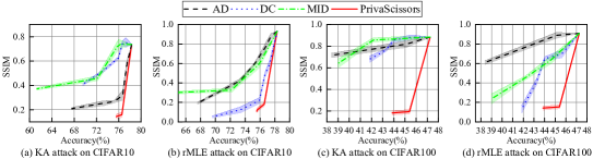
Figure 3: Results of model accuracy v.s. SSIM of reconstruction on CIFAR10 and CIFAR100 against rMLE and KA attack.

For defense against KA attacks, our PrivaScissors can reduce the SSIM of reconstruction to lower than 0.2 with a model accuracy drop of less than 2% for CIFAR10. In contrast, the other baselines drop model accuracy by more than 10% and cannot achieve the same defense effect even with an accuracy drop of more than 10%. Notably, the malicious server has more auxiliary data on CIFAR100 than CIFAR10, making the attack harder to defend on CIFAR100 to the baselines. However, PrivaScissors can still achieve an SSIM of lower than 0.2 with a model accuracy drop of less than 2%. We also evaluate our defense against the KA attack with a larger auxiliary dataset on the malicious server, and the results show that our defense can effectively defend against the KA attack when the server has more auxiliary samples. For defense against rMLE attacks, PrivaScissors achieves similar results of reducing the SSIM to lower than 0.2 with a model accuracy drop of less than 2% for CIFAR10 and 1% for CIFAR100, respectively, which outperforms the other baselines significantly.

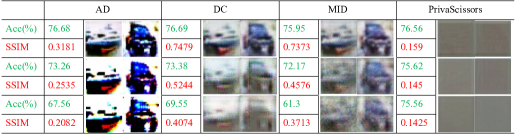
Figure 4: Images reconstructed by the KA attack on CIFAR10 under different defenses.

To perceptually demonstrate the effectiveness of our defense, we show the reconstructed images by the KA attack on CIFAR10 after applying baseline defenses and our defense in Fig. 4. It is shown that by applying the baseline defenses, the reconstructed images still contain enough information to be recognizable with the model accuracy of lower than 70%. For our method, the reconstructed images do not contain much information about the raw images, with the model accuracy higher than 76%.

5.3 Results of Prediction Protection

We evaluate PrivaScissors on two datasets against two attack methods. We set different defense levels for our methods (i.e., different $\lambda_{l}$ values in Eq. 9) and baselines to conduct multiple experiments to show the trade-off between the model accuracy and attack accuracy. The defense results against PMC and AMC attacks are shown in Fig. 5 and Fig. 6, respectively. To simulate the realistic settings in that the malicious server uses different model architectures to conduct MC attacks, we apply different model architectures (MLP & MLP_sim) for MC attacks.

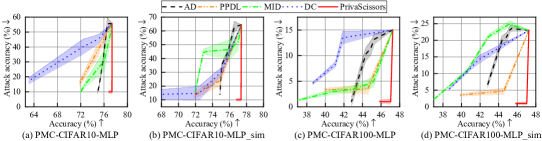
Figure 5: Results of model accuracy v.s. attack accuracy on CIFAR10 and CIFAR100 against PMC attack.

For defense against PMC on CIFAR10, PrivaScissors achieves 10% attack accuracy (equal to random guess) by sacrificing less than 0.5% model accuracy, while the other baselines suffer a model accuracy drop by more than 4% to achieve the same defense effect. Similarly, PrivaScissors achieves 1% attack accuracy on CIFAR100 by sacrificing less than 1% model accuracy, while the other baselines achieve the same defense effect by sacrificing more than 6% model accuracy.

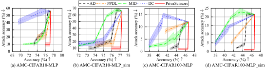
Figure 6: Results of model accuracy v.s. attack accuracy on CIFAR10 and CIFAR100 against AMC attack.

PrivaScissors also shows robustness against AMC. PrivaScissors achieves attack accuracy of the rate of random guess by sacrificing less than 1% and 0.5% model accuracy on CIFAR10 and CIFAR100, respectively. The other baselines achieve the same defense performance by sacrificing more than 5% and 4% model accuracy, respectively.

5.4 Integration of Data and Prediction protection

We have shown the compared results of data and prediction protection between PrivaScissors and the baselines in Sec. 5.2 and Sec. 5.3. In this section, we evaluate the integration of data and prediction protection of PrivaScissors. We set $\lambda_{d}$ and $\lambda_{l}$ between 0.05-0.4 and evaluate the defenses. The results of defense against the KA and PMC attacks on CIFAR10 and CIFAR100 are shown in Fig. 7. It is shown that PrivaScissors can effectively protect data and prediction simultaneously with less than a 2% accuracy drop for both datasets.

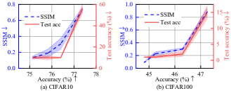
Figure 7: PrivaScissors against KA and PMC on CIFAR10 and CIFAR100.

6 Conclusion

We propose a defense method PrivaScissors, against privacy leakage in collaborative inference by reducing the mutual information between the model’s intermediate outcomes and the device’s data and predictions. The experimental results show that PrivaScissors can defend against data leakage and prediction leakage effectively. We also provide a theoretically certified robustness guarantee for PrivaScissors. In this paper, we focus on the scenario where there is only one edge device. Our defense can be easily applied to the collaborative inference scenario with multiple edge devices.

Appendix A Algorithm

Algorithm 1 Training algorithm of PrivaScissors. ${\color[rgb]{0,1,0}\leftarrow}$ means information is sent to the server; ${\color[rgb]{0,0,1}\leftarrow}$ means information is sent to the device; red steps are conducted on the cloud server.

1:Dataset $\left\{\left(x_{i},y_{i}\right)\right\}_{i=1}^{N}$; Learning rate $\eta$.

2:$\theta^{h};\theta^{e};\theta^{c};\psi;\phi$.

3:Initialize $\theta^{h},\theta^{e},\theta^{c},\psi,\phi$;

4:for a batch of data $\left\{\left(x_{i},y_{i}\right)\right\}_{i\in{\mathbb{B}}}$ do

5:    $\{r_{i}\}_{i\in{\mathbb{B}}}{\color[rgb]{0,1,0}\leftarrow}\{f^{h}_{\theta^{h}}\left(x_{i}\right)\}_{i\in{\mathbb{B}}}$;

6:    $\mathcal{L}_{d\_a}\leftarrow\frac{1}{|{\mathbb{B}}|}\sum\limits_{i\in{\mathbb{B}}}\log g_{\psi}\left(x_{i}|r_{i}\right)$;

7:    $\psi\leftarrow\psi+\eta\nabla_{\psi}\mathcal{L}_{d\_a}$;

8:    $\{z_{i}\}_{i\in{\mathbb{B}}}{\color[rgb]{0,0,1}\leftarrow}{\color[rgb]{1,0,0}\{f^{e}_{\theta^{e}}\left(r_{i}\right)\}_{i\in{\mathbb{B}}}}$;

9:    $\mathcal{L}_{c}\leftarrow\frac{1}{|{\mathbb{B}}|}\sum\limits_{i\in{\mathbb{B}}}\mathcal{L}\left(f^{c}_{\theta^{c}}\left(z_{i}\right),y_{i}\right)$;

10:    $\mathcal{L}_{l\_a}\leftarrow\frac{1}{|{\mathbb{B}}|}\sum\limits_{i\in{\mathbb{B}}}\log h_{\phi}\left(y_{i}|z_{i}\right)$;

11:    $\theta^{c}\leftarrow\theta^{c}-\eta\nabla_{\theta^{c}}\mathcal{L}_{c}$;

12:    $\phi\leftarrow\phi+\eta\nabla_{\phi}\mathcal{L}_{l\_a}$;

13:    $\{y_{n_{i}^{\prime}}\}_{i\in{\mathbb{B}}}\leftarrow$ randomly sample $\{y_{n_{i}^{\prime}}\}_{i\in{\mathbb{B}}}$ from $\{y_{i}\}_{i\in[N]}$;

14:    $\{x_{k_{i}^{\prime}}\}_{i\in{\mathbb{B}}}\leftarrow$ randomly sample $\{x_{k_{i}^{\prime}}\}_{i\in{\mathbb{B}}}$ from $\{x_{i}\}_{i\in[N]}$;

15:    $\mathcal{L}_{d\_r}\leftarrow\frac{1}{|{\mathbb{B}}|}\sum\limits_{i\in{\mathbb{B}}}-\log g_{\psi}\left(x_{k_{i}^{\prime}}|r_{i}^{2}\right)$;

16:    $\mathcal{L}_{l\_r}\leftarrow\frac{1}{|{\mathbb{B}}|}\sum\limits_{i\in{\mathbb{B}}}-\log h_{\phi}\left(y_{n_{i}^{\prime}}|z_{i}^{2}\right)$;

17:    $\{\nabla_{z_{i}}\mathcal{L}\}_{i\in{\mathbb{B}}}{\color[rgb]{0,1,0}\leftarrow}\{\nabla_{z_{i}}\left[(1-\lambda_{d}-\lambda_{l})\mathcal{L}_{c}+\lambda_{l}\mathcal{L}_{l\_a}+\lambda_{l}\mathcal{L}_{l\_r}+\lambda_{d}\mathcal{L}_{d\_a}+\lambda_{d}\mathcal{L}_{d\_r}\right]\}_{i\in{\mathbb{B}}}$;

18:    ${\color[rgb]{1,0,0}{\nabla_{\theta^{e}}\mathcal{L}\leftarrow\frac{1}{|{\mathbb{B}}|}\sum\limits_{i\in{\mathbb{B}}}}\nabla_{z_{i}}\mathcal{L}\nabla_{\theta^{e}}{z_{i}}}$

19:    ${\color[rgb]{1,0,0}\theta^{e}\leftarrow\theta^{e}-\eta\nabla_{\theta^{e}}\mathcal{L}}$;

20:    $\{\nabla_{r_{i}}\mathcal{L}\}_{i\in{\mathbb{B}}}{\color[rgb]{0,0,1}\leftarrow}{\color[rgb]{1,0,0}\{\nabla_{z_{i}}\mathcal{L}\nabla_{r_{i}}{z_{i}}\}_{i\in{\mathbb{B}}}}$;

21:    ${\nabla_{\theta^{h}}\mathcal{L}\leftarrow\frac{1}{|{\mathbb{B}}|}\sum\limits_{i\in{\mathbb{B}}}}\nabla_{r_{i}}\mathcal{L}\nabla_{\theta^{h}}{r_{i}}$;

22:    $\theta^{h}\leftarrow\theta^{h}-\eta\nabla_{\theta^{h}}\mathcal{L}$;

23:end for

Appendix B Proofs of theorems

Proof 1

According to Corollary 3.3 in [23], we have:

$$\text{I}({\textnormal{z}};{\textnormal{y}})<\text{I}_{\text{vCLUB}}({\textnormal{z}};{\textnormal{y}})+\text{KL}(p(y|z)||h_{\phi}(y|z)).$$ (16)

Then we have

$$\text{I}({\textnormal{z}};{\textnormal{y}})=\mathbb{E}_{p\left({\textnormal{z}},{\textnormal{y}}\right)}\log p\left({\textnormal{y}}|{\textnormal{z}}\right)-\mathbb{E}_{p\left({\textnormal{y}}\right)}\log p\left({\textnormal{y}}\right)<\epsilon,$$ (17)

where $\epsilon=\text{I}_{\text{vCLUB}}({\textnormal{z}};{\textnormal{y}})+\text{KL}(p(y|z)||h_{\phi}(y|z))$. With the samples $\{x_{i},y_{i}\}$, $\text{I}({\textnormal{z}};{\textnormal{y}})$ has an unbiased estimation as:

$$\frac{1}{N}\sum\limits_{i=1}^{N}\log p(y_{i}|z_{i})-\frac{1}{N}\sum\limits_{i=1}^{N}\log p(y_{i})<\epsilon.$$ (18)

Suppose the adversary has an optimal model $h^{m}$ to estimate $p(y_{i}|z_{i})$ such that $h^{m}(y_{i}|z_{i})=p(y_{i}|z_{i})$ for any $i$, then

$$\frac{1}{N}\sum\limits_{i=1}^{N}\log h^{m}(y_{i}|z_{i})-\frac{1}{N}\sum\limits_{i=1}^{N}\log p(y_{i})<\epsilon.$$ (19)

For classification tasks, we have

$$\frac{1}{N}\sum\limits_{i=1}^{N}\text{CE}\left[h^{m}(z_{i}),y_{i}\right]>\text{CE}_{random}-\epsilon.$$ (20)

Proof 2

Similar with Eq. 18, we derive the following for data protection:

$$\frac{1}{N}\sum\limits_{i=1}^{N}\log p(x_{i}|r_{i})-\frac{1}{N}\sum\limits_{i=1}^{N}\log p(x_{i})<\epsilon,$$ (21)

where $\epsilon=\text{I}_{\text{vCLUB}}({\textnormal{r}};{\textnormal{x}})+\text{KL}(p(x|r)||g_{\psi}(x|r))$. Following the assumption that $p(x|r)$ follows a Gaussian distribution of variance 1, suppose the adversary obtains an optimal estimator $g_{m}$ of the mean of $p(x|r)$ such that $g^{m}(x_{i}|r_{i})=p(x_{i}|r_{i})$ for any $i$. Then we have

$$\frac{1}{N}\sum\limits_{i=1}^{N}\log g^{m}(x_{i}|r_{i}) <\frac{1}{N}\sum\limits_{i=1}^{N}\log p(x_{i})+\epsilon$$ (22)

$$\frac{1}{N}\sum\limits_{i=1}^{N}\log\frac{1}{\sqrt{2\pi}}e^{-\frac{1}{2}\left[x_{i}-g^{m}(r_{i})\right]^{T}\left[x_{i}-g^{m}(r_{i})\right]} <\frac{1}{N}\sum\limits_{i=1}^{N}\log p(x_{i})+\epsilon$$

$$-\frac{1}{N}\sum\limits_{i=1}^{N}\log\sqrt{2\pi}-\frac{1}{2N}\sum\limits_{i=1}^{N}\left[x_{i}-g^{m}(r_{i})\right]^{T}\left[x_{i}-g^{m}(r_{i})\right] <\frac{1}{N}\sum\limits_{i=1}^{N}\log p(x_{i})+\epsilon$$

$$\frac{1}{2N}\sum\limits_{i=1}^{N}\left[x_{i}-g^{m}(r_{i})\right]^{T}\left[x_{i}-g^{m}(r_{i})\right] >\frac{1}{N}\sum\limits_{i=1}^{N}\log\frac{\sqrt{2\pi}}{p(x_{i})}-\epsilon.$$

We denote the dimension of x as Q and $\frac{1}{N}\sum\limits_{i=1}^{N}\log\frac{\sqrt{2\pi}}{p(x_{i})}$ as $\kappa$. Then we have

$$\frac{1}{N}\sum\limits_{i=1}^{N}\text{MSE}\left[g^{m}(r_{i}),x_{i}\right]>\frac{2(\kappa-\epsilon)}{Q}.$$ (23)

References

- [1] G. Li, L. Liu, X. Wang, X. Dong, P. Zhao, and X. Feng, “Auto-tuning neural network quantization framework for collaborative inference between the cloud and edge,” in Artificial Neural Networks and Machine Learning–ICANN 2018: 27th International Conference on Artificial Neural Networks, Rhodes, Greece, October 4-7, 2018, Proceedings, Part I 27, pp. 402–411, Springer, 2018.
- [2] N. Shlezinger, E. Farhan, H. Morgenstern, and Y. C. Eldar, “Collaborative inference via ensembles on the edge,” in ICASSP 2021-2021 IEEE International Conference on Acoustics, Speech and Signal Processing (ICASSP), pp. 8478–8482, IEEE, 2021.
- [3] H. Zhou, W. Zhang, C. Wang, X. Ma, and H. Yu, “Bbnet: a novel convolutional neural network structure in edge-cloud collaborative inference,” Sensors, vol. 21, no. 13, p. 4494, 2021.
- [4] Z. He, T. Zhang, and R. B. Lee, “Model inversion attacks against collaborative inference,” in Proceedings of the 35th Annual Computer Security Applications Conference, pp. 148–162, 2019.
- [5] Z. He, T. Zhang, and R. B. Lee, “Attacking and protecting data privacy in edge–cloud collaborative inference systems,” IEEE Internet of Things Journal, vol. 8, no. 12, pp. 9706–9716, 2020.
- [6] L. Zhu, Z. Liu, and S. Han, “Deep leakage from gradients,” Advances in neural information processing systems, vol. 32, 2019.
- [7] B. Zhao, K. R. Mopuri, and H. Bilen, “idlg: Improved deep leakage from gradients,” arXiv preprint arXiv:2001.02610, 2020.
- [8] C. Fu, X. Zhang, S. Ji, J. Chen, J. Wu, S. Guo, J. Zhou, A. X. Liu, and T. Wang, “Label inference attacks against vertical federated learning,” in 31st USENIX Security Symposium (USENIX Security 22), pp. 1397–1414, 2022.
- [9] O. Li, J. Sun, X. Yang, W. Gao, H. Zhang, J. Xie, V. Smith, and C. Wang, “Label leakage and protection in two-party split learning,” arXiv preprint arXiv:2102.08504, 2021.
- [10] Y. Liu, Z. Yi, Y. Kang, Y. He, W. Liu, T. Zou, and Q. Yang, “Defending label inference and backdoor attacks in vertical federated learning,” arXiv preprint arXiv:2112.05409, 2021.
- [11] T. Wang, Y. Zhang, and R. Jia, “Improving robustness to model inversion attacks via mutual information regularization,” in Proceedings of the AAAI Conference on Artificial Intelligence, vol. 35, pp. 11666–11673, 2021.
- [12] T. Zou, Y. Liu, and Y.-Q. Zhang, “Mutual information regularization for vertical federated learning,” arXiv preprint arXiv:2301.01142, 2023.
- [13] X. Luo, Y. Wu, X. Xiao, and B. C. Ooi, “Feature inference attack on model predictions in vertical federated learning,” in 2021 IEEE 37th International Conference on Data Engineering (ICDE), pp. 181–192, IEEE, 2021.
- [14] X. Jiang, X. Zhou, and J. Grossklags, “Comprehensive analysis of privacy leakage in vertical federated learning during prediction,” Proceedings on Privacy Enhancing Technologies, vol. 2022, no. 2, pp. 263–281, 2022.
- [15] X. Jin, P.-Y. Chen, C.-Y. Hsu, C.-M. Yu, and T. Chen, “Cafe: Catastrophic data leakage in vertical federated learning,” Advances in Neural Information Processing Systems, vol. 34, pp. 994–1006, 2021.
- [16] M. Fredrikson, S. Jha, and T. Ristenpart, “Model inversion attacks that exploit confidence information and basic countermeasures,” in Proceedings of the 22nd ACM SIGSAC conference on computer and communications security, pp. 1322–1333, 2015.
- [17] J. Sun, A. Li, B. Wang, H. Yang, H. Li, and Y. Chen, “Soteria: Provable defense against privacy leakage in federated learning from representation perspective,” in Proceedings of the IEEE/CVF conference on computer vision and pattern recognition, pp. 9311–9319, 2021.
- [18] J. Geiping, H. Bauermeister, H. Dröge, and M. Moeller, “Inverting gradients-how easy is it to break privacy in federated learning?,” Advances in Neural Information Processing Systems, vol. 33, pp. 16937–16947, 2020.
- [19] H. Yin, A. Mallya, A. Vahdat, J. M. Alvarez, J. Kautz, and P. Molchanov, “See through gradients: Image batch recovery via gradinversion,” in Proceedings of the IEEE/CVF Conference on Computer Vision and Pattern Recognition, pp. 16337–16346, 2021.
- [20] L. Melis, C. Song, E. De Cristofaro, and V. Shmatikov, “Exploiting unintended feature leakage in collaborative learning,” in 2019 IEEE symposium on security and privacy (SP), pp. 691–706, IEEE, 2019.
- [21] K. Chaudhuri and D. Hsu, “Sample complexity bounds for differentially private learning,” in Proceedings of the 24th Annual Conference on Learning Theory, pp. 155–186, JMLR Workshop and Conference Proceedings, 2011.
- [22] B. Ghazi, N. Golowich, R. Kumar, P. Manurangsi, and C. Zhang, “Deep learning with label differential privacy,” Advances in neural information processing systems, vol. 34, pp. 27131–27145, 2021.
- [23] P. Cheng, W. Hao, S. Dai, J. Liu, Z. Gan, and L. Carin, “Club: A contrastive log-ratio upper bound of mutual information,” in International conference on machine learning, pp. 1779–1788, PMLR, 2020.
- [24] C. Fu, X. Zhang, S. Ji, J. Chen, J. Wu, S. Guo, J. Zhou, A. X. Liu, and T. Wang, “Label inference attacks against vertical federated learning,” in 31st USENIX Security Symposium (USENIX Security 22), (Boston, MA), pp. 1397–1414, USENIX Association, Aug. 2022.
- [25] R. Shokri and V. Shmatikov, “Privacy-preserving deep learning,” in Proceedings of the 22nd ACM SIGSAC Conference on Computer and Communications Security, CCS ’15, (New York, NY, USA), p. 1310–1321, Association for Computing Machinery, 2015.