Neural Scene Chronology

Abstract

In this work, we aim to reconstruct a time-varying 3D model, capable of rendering photo-realistic renderings with independent control of viewpoint, illumination, and time, from Internet photos of large-scale landmarks. The core challenges are twofold. First, different types of temporal changes, such as illumination and changes to the underlying scene itself (such as replacing one graffiti artwork with another) are entangled together in the imagery. Second, scene-level temporal changes are often discrete and sporadic over time, rather than continuous. To tackle these problems, we propose a new scene representation equipped with a novel temporal step function encoding method that can model discrete scene-level content changes as piece-wise constant functions over time. Specifically, we represent the scene as a space-time radiance field with a per-image illumination embedding, where temporally-varying scene changes are encoded using a set of learned step functions. To facilitate our task of chronology reconstruction from Internet imagery, we also collect a new dataset of four scenes that exhibit various changes over time. We demonstrate that our method exhibits state-of-the-art view synthesis results on this dataset, while achieving independent control of viewpoint, time, and illumination. Code and data are available at https://zju3dv.github.io/neusc/.

Figure 1: Chronology reconstruction. Given timestamped Internet photos (a) of a landmark that has changed significantly over the years (e.g., 5Pointz, NYC, the collective graffiti art project shown above), our method can reconstruct a time-varying 3D model, and render photo-realistic images (b) with independent control of viewpoint, time (c) and illumination (d). Photos by Flickr users Ryan Brown, DaniGMX, DJ Leekee, Diff Graff, Lee Smith, James Prochnik, Verity Rollins Photo under CC BY.

1 Introduction

If we revisit a space we once knew during our childhood, it might not be as we remembered it. The buildings may have weathered, or have been newly painted, or may have been replaced entirely. Accordingly, there is no such thing as a single, authoritative 3D model of a scene—only a model of how it existed at a given instant in time. For a famous landmark, Internet photos can serve as a kind of chronicle of that landmark’s state over time, if we could organize the information in those photos in a coherent way. For instance, if we could reconstruct a time-varying 3D model, then we could revisit the scene at any desired point in time.

In this work, we explore this problem of chronology reconstruction, revisiting the work on Scene Chronology from nearly a decade ago [30]. As in that work, we seek to use Internet photos to build a 4D model of a scene, from which we can dial in any desired time (within the time interval where we have photos). However, the original Scene Chronology work was confined to reconstructing planar, rectangular scene elements, leading to limited photo-realism. We can now revisit this problem with powerful neural scene representations, inspired by methods such as NeRF in the Wild [29]. However, recent neural reconstruction methods designed for Internet photos assume that the underlying scene is static, which works well for landmarks with a high degree of permanence, but fails for other scenes, like New York’s Times Square, that feature more ephemeral elements like billboards and advertisements.

However, we find that adapting neural reconstruction methods [29] to the chronology reconstruction problem has many challenges, and that straightforward extensions do not work well. For instance, augmenting a neural radiance field (NeRF) model with an additional time input $t$, and fitting the resulting 4D radiance field to a set of images with timestamps yields temporally oversmoothed models, where different scene appearances over time are blended together, forming ghosted content; such a model underfits the temporal signal. On the other hand, applying standard positional encoding [34] to the time input overfits the temporal signal, conflating transient appearance changes due to factors like illumination with longer-term, sporadic changes to the underlying scene itself.

Instead, we seek a model that can disentangle transient, per-image changes from longer-term, scene-level changes, and that allows for independent control of viewpoint, time, and illumination at render-time. Based on the observation that scene-level content changes are often sudden, abrupt “step function”-like changes (e.g., a billboard changing from one advertisement to another), we introduce a novel encoding method for time inputs that can effectively model piece-wise constant scene content over time, and pair this method with a per-image illumination code that models transient appearance changes. Accordingly, we represent 4D scene content as a multi-layer perceptron (MLP) that stores density and radiance at each space-time $(x,y,z,t)$ scene point, and takes an illumination code as a side input. The time input $t$ to this MLP is encoded with our proposed step function encoding that models piecewise constant temporal changes. When fit to a set of input images, we find that our representation can effectively factor different kinds of temporal effects, and can produce high-quality renderings of scenes over time.

To evaluate our method, we collect a dataset of images from Flickr and calibrate them using COLMAP, resulting in 52K successfully registered images. These photos are sourced from four different scenes, including dense tourist areas, graffiti meccas, and museums, building upon the datasets used in Scene Chronology. These scenes feature a variety of elements that change over time, including billboards, graffiti art, and banners. Experiments on these scenes show that our method outperforms current state-of-the-art methods and their extensions to space-time view synthesis [29, 6]. We also present a detailed ablation and analysis of our proposed time encoding method.

In summary, our work makes the following contributions:

• To the best of our knowledge, ours is the first work to achieve photo-realistic chronology reconstruction, allowing for high-quality renderings of scenes with controllable viewpoint, time, and illumination.

• We propose a novel encoding method that can model abrupt content changes without overfitting to transient factors. This leads to a fitting procedure that can effectively disentangle illumination effects from content changes in the underlying scene.

• We benchmark the task of chronology reconstruction from Internet photos and make our dataset and code available to the research community.

2 Related Work

3D/4D reconstruction from Internet photos. The typical 3D reconstruction pipeline for Internet photos involves first recovering camera poses and a sparse point cloud using Structure from Motion (SfM) methods [51, 1, 46, 44, 52], then computing a dense reconstruction using Multi-View Stereo (MVS) algorithms [13, 11, 10, 47]. However, these methods assume the scene to be largely static, and are unable to produce coherent models for scenes with large-scale appearance changes over time. To extend these methods to achieve 4D reconstruction, Schindler and Dellaert developed a method that takes photos of a city over time, and reasons probabilistically about visibility and existence of objects like buildings that may come and go across decades [45]. Most related to our work, Scene Chronology extends MVS methods [48] to 4D by clustering reconstructed 3D points into space-time cuboids [30]. However, it can only reconstruct and render planar regions, leading to limited photo-realism. To handle more complex geometry, Martin-Brualla et al. represent scene geometry using time-varying depth maps, allowing their method to generate high-quality time-lapse videos [28, 27]. However, this depth map–based representation limits the range of camera viewpoints their method can synthesize. In our work, we tackle these challenges and devise a new method that can handle large-scale scenes with complex geometry, and can generate large camera motions.

Novel view synthesis. Early methods achieve novel view synthesis through light field interpolation [14, 18, 7] or image-based rendering [60, 4, 9, 17]. Recently, neural scene representations [35, 36, 31, 50, 33, 55, 57] have shown unprecedented view synthesis quality. Of particular interest is NeRF [34], which represents radiance fields using a multi-layer perceptron (MLP) and achieves impressive rendering results. Many works [20, 58, 40, 37, 38, 24, 59, 19, 56, 8, 39, 12, 43, 22] extend NeRF to model dynamic scenes with moving objects given a monocular or multi-view video as input. In our work, we focus on a different type of 4D view synthesis problem that involves modeling unstructured Internet photo collections capturing scenes that exhibit substantial appearance changes over time.

Neural rendering from Internet photos. One challenge of rendering from Internet photos is handling varying, unknown illumination present in the image collection. Recently, several neural rendering methods demonstrate promising results on rendering static landmarks while allowing for control of illumination effects [32, 23]. In particular, NeRF-W [29] conditions a reconstructed neural radiance field on a learnable per-image illumination vector, thereby factoring out per-image illumination effects. Chen et al. [6] propose a CNN module for predicting an illumination vector from an image, enabling transfer of illumination from unseen images to the model. Sun et al. [53] build on NeRF-W to reconstruct 3D meshes from a collection of Internet photos. Finally, Zhao and Yang et al. [2] and Rudnev et al. [42] enable outdoor scene relighting based on neural radiance fields. However, these methods are limited to primarily static landmarks like the Brandenburg Gate, and cannot handle scenes with substantial changes over time like Times Square.

Modeling temporal signals. One useful type of data for modeling temporal signals is time-lapse videos from stationary cameras, which provide organized visual information for scene understanding and factorization. Many previous methods [25, 21, 54] show how to factor temporally-varying factors (e.g., illumination) from permanent scene factors (e.g., geometry and reflectance) from time-lapse videos. More recently, [16] introduces a method that disentangles time-lapse sequences in a way that allows separate, after-the-fact control of overall trends, cyclic effects, and random effects in the images. In our work, we focus on a more challenging setup, where our input is unstructured Internet photos from different viewpoints, and where we aim to synthesize novel views in addition to factorizing different temporal components.

3 Method

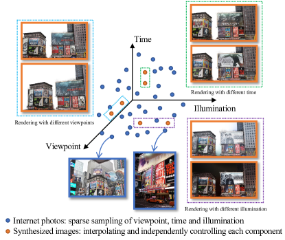
Figure 2: Problem illustration. Given an Internet photo collection of a scene, each image can be thought of as a sample in a high-dimensional space consisting of entangled information, including viewpoint, time, and lighting effects. The photo collection represents a sparse sampling of this space. Our goal is to recover a 4D scene representation from this sparse sampling, and to enable interpolation in this high-dimensional space with disentanglement and independent control of viewpoint, time, and lighting.

The input to our method is a collection of Internet photos of a landmark (e.g., Times Square) with known timestamps and camera poses. Our goal is to recover a 4D scene representation that can be used to render photo-realistic images of that scene with independently controlled viewpoint, time, and lighting effects as illustrated in Fig. 2. This is a challenging problem because different kinds of temporal changes, including scene content changes (changes to the scene itself) and lighting variation (e.g., time of day) are entangled in each image, but must be disentangled in the scene representation to enable independent control over each temporal component. Furthermore, content changes in our target scenes often happen suddenly, meaning that the scene representation must be able to model discrete, sporadic changes over time.

To tackle this problem, we propose a new 4D scene representation that can disentangle viewpoint, lighting effects, and time. Our key observation is that the scene content often changes less frequently over time and remains nearly constant in-between changes, whereas illumination changes much more frequently and sometimes dramatically. For example, the graffiti in 5Pointz (see Fig. 1) may only be replaced every few months, but illumination can change over the course of a few hours. Motivated by this observation, we model illumination variation with a per-image illumination embedding, and model the underlying 4D scene content using an MLP with time as input. We introduce our scene representation in Sec. 3.1. To model piece-wise constant temporal content with abrupt transitions, we propose a novel encoding method in Sec. 3.2 that utilizes the behavior of the step function, i.e., remaining consistent given a continuous input, while allowing abrupt changes at transition points.

Figure 3: Visual ablation of the proposed time encoding. Given a video rendered at a fixed viewpoint through several years, we compute the Mean Squared Error (MSE) between every pair of consecutive frames. The vertical and horizontal axes represent MSE and time, respectively. For a scene with sporadic changes, we expect to see infrequent “deltas” in this MSE plot. We observe that our method indeed 1) recovers the transition points of scene changes and 2) stays consistent (zero MSE) at other times. With no time encoding, 1) is violated, leading to blended, ghosted visual content (top left), and with positional encoding, 2) is violated, leading to temporal flicker (top middle). Please see our supplemental video for animated results.

3.1 4D Reconstruction from Internet Photos

Given a posed image collection $\{\mathcal{I}_{i}\}_{i=1}^{N}$ with timestamps $\{t_{i}\}_{i=1}^{N}$, we represent the 4D scene as a time-varying neural field. To disentangle changes to the underlying scene from the varying and unknown per-image illumination, each image $\mathcal{I}_{i}$ is assigned a learnable illumination embedding vector $\boldsymbol{\ell}_{i}$, which is meant to encode the illumination present in that view. Formally, given a space-time point $(\mathbf{x},t_{i})$ with 3D spatial coordinate $\mathbf{x}$ and time $t_{i}$, along with an illumination code $\boldsymbol{\ell}_{i}$ and view direction $\mathbf{d}$, we use an MLP denoted by $\mathbf{F}$ to encode its radiance $\mathbf{c}$ and volume density $\sigma$ as follows:

$$\mathbf{c},\sigma=\mathbf{F}(\mathbf{x},t_{i},\boldsymbol{\ell}_{i},\mathbf{d}).$$ (1)

Following NeRF [34], the input spatial coordinates $\mathbf{x}$ and ray direction $\mathbf{d}$ are mapped to higher-dimensional vectors via a fixed positional encoding function. For simplicity, we assume that the scene geometry is mostly constant, and only the appearance changes over time, but our method could also be extended to handle time-varying geometry. Therefore the model in Eq. 1 can be divided into a static, time-invariant geometric model and a time-aware appearance model, denoted by $\mathbf{F}_{\text{geo}}$ and $\mathbf{F}_{\text{app}}$, respectively:

$$\mathbf{v},\sigma=\mathbf{F}_{\text{geo}}(\mathbf{x}),$$ (2)

$$\mathbf{c}=\mathbf{F}_{\text{app}}(\mathbf{x},\mathbf{v},t_{i},\boldsymbol{\ell}_{i},\mathbf{d}).$$ (3)

$\mathbf{F}_{\text{geo}}$ models static geometry, and is parameterized by just the input 3D position $\mathbf{x}$, while $\mathbf{F}_{\text{app}}$ models time-dependent appearance, and depends on the space-time point $(\mathbf{x},t_{i})$, illumination embedding $\boldsymbol{\ell}_{i}$, view direction $\mathbf{d}$, and the intermediate geometry feature vector $\mathbf{v}$ produced by $\mathbf{F}_{\text{geo}}$. Please refer to the supplementary material for additional details about the model architecture.

From this scene representation, we can render images using volume rendering, and optimize the scene representation by comparing these rendered images to the known input views via an image reconstruction loss. Specifically, given an input image $\mathcal{I}_{i}$ with timestamp $t_{i}$, we compute the color of a ray $\mathbf{r}(s)=\mathbf{o}+s\mathbf{d}$, emitted from the camera center $\mathbf{o}$ through a given pixel in direction $\mathbf{d}$ as follows: We use stratified sampling to sample a set of quadrature points $\{s_{k}\}_{k=1}^{K}$ between $s_{n}$ and $s_{f}$, the near and far bounds along the ray. Then, given the illumination embedding $\boldsymbol{\ell}_{i}$ and timestamp $t_{i}$ of image $\mathcal{I}_{i}$, we can compute the color $\mathbf{c}(s_{k},t_{i},\boldsymbol{\ell}_{i})$ and density $\sigma(s_{k})$ of each sample $s_{k}$ given our scene representation. We then accumulate these points using volume rendering, as in NeRF [34], yielding the expected color $\hat{\mathbf{C}}(\mathbf{r},t_{i},\boldsymbol{\ell}_{i})$:

$$\hat{\mathbf{C}}(\mathbf{r},t_{i},\boldsymbol{\ell}_{i})=\sum_{k=1}^{K}T(s_{k})\alpha(\sigma(s_{k})\delta_{k})\mathbf{c}(s_{k},t_{i},\boldsymbol{\ell}_{i}),$$ (4)

$$\text{where}{\quad}T(s_{k})=\text{exp}\left(-\sum_{k^{\prime}=1}^{k-1}\sigma(s_{k^{\prime}})\delta_{k^{\prime}}\right),$$ (5)

where $\alpha(x)=1-\text{exp}(-x)$, and $\delta_{k}=s_{k+1}-s_{k}$. We minimize the sum of squared error between the rendered and ground truth pixels:

$$\mathcal{L}=\sum_{(\mathbf{r},i)\in\Omega}\|\mathbf{C}_{i}(\mathbf{r})-\hat{\mathbf{C}}(\mathbf{r},t_{i},\boldsymbol{\ell}_{i})\|_{2}^{2},$$ (6)

where $\mathbf{C}_{i}(\mathbf{r})$ is the observed pixel color in image $\mathcal{I}_{i}$ with timestamp $t_{i}$, and $\Omega$ is the set of all the sampled pixels from the image collection $\{\mathcal{I}_{i}\}_{i=1}^{N}$.

3.2 Step Function Encoding for Time Input

The method described above serves as a baseline to model a 4D scene from Internet photos. However, we found that this baseline cannot model temporal changes in the target scene well. Specifically, temporal appearance changes in man-made scenes are often abrupt, such as a new billboard or sign in Times Square, or a new graffiti artwork in an art mecca like 5Pointz. In contrast, the baseline above tends to average over temporal content changes, resulting in a cross-fade transition in time between two appearance states, rather than a sharp, sudden transition. Fig. 3 shows an example where this baseline (denoted “without encoding” in the figure) produces a ghosted blend of two temporally consecutive graffiti artworks. This finding is consistent with NeRF’s observation that standard coordinate inputs cannot model high-frequency signals [34]. To address this issue, NeRF uses positional encoding to map input spatial coordinates to a high-frequency signal. However, we found that applying positional encoding to the time input causes the network to not only fit the underlying appearance changes in the scene, but also overfit to per-image lighting effects. In other words, it fails to disentangle these two components and leads to severe flickering artifacts over time, as shown in Fig. 3.

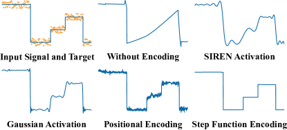
Figure 4: Fitting an MLP to a noisy piecewise constant 1D signal. Given the noisy orange data points (uniform noise), we aim to recover the clean blue curve shown in the upper left plot. We present the results of fitting the input data using an MLP with different encoding methods and activation functions. Our proposed step function encoding achieves the best results, recovering the discrete, sporadic changes in the signal without over-fitting to noise.

To address this problem, we present a novel encoding method based on a step function. The step function has the desirable property that the output mostly stays constant with respect to the input, except when it changes abruptly at a transition point. Therefore, we consider using the step function defined below as the encoding function for time $t$:

$$h(t)=\begin{cases}0&\text{if \;}t\leq u\\ 1&\text{if \;}t>u\end{cases},$$ (7)

where $u$ is a learnable parameter representing the transition point. However, $h(t)$ is discontinuous and the gradient for $u$ is not well-defined. We therefore use a smooth approximation to $h(t)$ to make it differentiable, denoted as $\bar{h}(t)$:

$$\bar{h}(t)=\begin{cases}\frac{1}{2}\text{exp}(\frac{t-u}{\beta})&\text{if \;}t\leq u\\ 1-\frac{1}{2}\text{exp}(\frac{-(t-u))}{\beta})&\text{if \;}t>u\end{cases},$$ (8)

where $\beta$ is a learnable parameter representing the steepness of the step function. In practice, $u$ is randomly initialized from zero to one and $\beta$ is initialized to 0.3. Our encoding method uses a vector of step functions, denoted as $\mathbf{H}(t)$, each with its own learned transition point, to express multiple transition points. $u$ and $\beta$ are jointly learned during training. We experimentally show that we can simply set the dimension of this vector to a large number that exceeds the expected number of scene transitions.

To illustrate the effectiveness of our proposed encoding function, we compare it with different encoding functions on a toy 1-D fitting experiment in Fig. 4. Baseline methods either overfit the noise (positional encoding [34], Gaussian [41]) or underfit the discrete, sporadic changes (without encoding, SIREN [49]). In contrast, our step function encoding correctly recovers the sharp changes in the signal by approximating real step functions with small $\beta$ parameters. Note that Gaussian and SIREN are used as the activation layer of a network, while our method and positional encoding are used to modulate the input.

3.3 Implementation Details

Learning scene appearance with parametric encoding. Using an implicit representation to reconstruct a large scene featuring content changes over time requires a large model capacity. While we could simply increase the size of the MLP, this strategy incurs a linear increase in training and rendering time. Motivated by Neural Sparse Voxel Fields (NSVF) [26], we adopt a parametric encoding which adds additional trainable parameters for scene appearance to effectively increase model capacity without introducing as much overhead. Observing that our target man-made scenes often satisfy the Manhattan world assumption, we use a tri-plane structure to arrange additional trainable parameters [3], which we found to be compact and expressive in our experiments. Specifically, we define three learnable feature planes: $\mathbf{E}_{xy}$, $\mathbf{E}_{yz}$, $\mathbf{E}_{xz}$. Each feature plane has a resolution of $D\times D\times B$, where $D$ and $B$ denote the spatial resolution and number of feature channels, respectively. Given a 3D point $\mathbf{p}$, we project it onto three axis-aligned orthogonal planes to obtain $\mathbf{p}_{xy},\mathbf{p}_{yz},\mathbf{p}_{xz}$. We can fetch the feature $\mathbf{f}_{xy}=\textbf{interp}(\mathbf{E}_{xy},\mathbf{p}_{xy})$, where interp is a linear interpolation operation. The same method can be applied to obtain $\mathbf{f}_{yz}$ and $\mathbf{f}_{xz}$. The appearance parametric encoding for $\mathbf{p}$ is defined as the concatenation of $\mathbf{f}_{xy}$, $\mathbf{f}_{yz}$ and $\mathbf{f}_{xz}$.

Handling transient objects. Learning a scene representation using Internet photos with transient objects may introduce 3D inconsistencies. To solve this problem, we employ a pretrained semantic segmentation model [5] to identify pixels of transient objects (e.g., pedestrians) and exclude these pixels during training. However, a segmentation model may not effectively filter out all transient pixels. To handle the remaining transient pixels, we use an MLP to predict whether each pixel in each image is a transient object. We learn it using the uncertainty loss, reducing the effect of transient pixels during training models as demonstrated in [6].

Other details. Our model includes an 8-layer MLP with 256 neurons for each layer as its backbone, and a 4-layer MLP as its appearance head. Our model is trained with an initial learning rate of $5e$-$4$, which is reduced to $5e$-$5$ after 800k iterations. At each iteration, we randomly sample $1024$ rays from an image. Following NeRF [34], we train our two models using the coarse-to-fine sampling strategy with $64$ and $128$ points for each ray in the coarse and fine levels, respectively. The model tends to converge after about 800k iterations, which takes about $40$ hours on an RTX 3090 GPU.

	Times Square	Akihabara	5Pointz	The Met
# Retrieved images	289,794	105,445	23,628	186,663
# Calibrated images	29,629	13,671	6,503	2,184
# Selected images	5,965	1,078	3,521	2,127

Table 1: Dataset statistics. We collect four scenes for evaluation. For each scene, we first retrieve photos from the Internet, then run COLMAP to calibrate them and reconstruct a sparse point cloud. After calibration, we choose a region of interest from the point cloud and select the corresponding images as input to our method.

4 Experiments

4.1 Experimental Setup

Datasets. We collect four scenes from Flickr that include two commercial tourist areas (Times Square and Akihabara), a graffiti mecca (5Pointz), and a museum (the Metropolitan Museum of Art aka the Met). The two commercial areas feature an array of billboards and other elements that change over time. 5Pointz is an outdoor space where artists paint graffiti art over time, each piece replacing (or augmenting) a previous one. The Met has a varying array of banners and signs advertising different exhibitions. For each scene, we run COLMAP to recover camera parameters and a sparse point cloud. Due to the large number of input images, running COLMAP on some of these scenes can take weeks on a cluster with multiple servers. We will release our processed data and data processing scripts as a resource for the community. Note that whole calibrated scenes, such as Times Square, can be excessively large for reconstruction using implicit representations. Instead, we perform view synthesis experiments on a region of the scene. Tab. 1 summarizes these datasets. We include visualizations of the reconstructed models and the selected regions, along with data processing details, in the supplemental material.

Metrics. To measure view synthesis quality, we randomly select a few dozen images per scene as a test set. To ensure the validity of our evaluation, we visually inspect the images in the test set and remove those that have excessive noise or that do not align with the intended task, such as black and white photos or images that are primarily portraits. For the remaining test images, there may still be some transient objects present. We manually annotate masks for these objects and ignore them during evaluation. Following NeRF-W [29], we use half of the valid pixels of each image to finetune the illumination embedding and the other half for testing PNSR/SSIM/LPIPS metrics. Please refer to the supplemental material for additional details.

	Act. func. / Freq.  / Dim.	Temporal stability		View synthesis quality
		Mean $\downarrow$	Entropy $\downarrow$	PSNR $\uparrow$	SSIM $\uparrow$	LPIPS $\downarrow$
w/o. Time	-	N/A	N/A	18.18	0.572	0.461
w/o. Encoding	-	0.116	5.314	20.54	0.719	0.296
Learned Latent	-	11.04	5.590	20.95	0.731	0.291
Activation	SIREN[49]	0.101	5.552	20.54	0.696	0.330
	Gaussian[41]	0.088	5.512	20.28	0.704	0.315
Positional Encoding	5	0.247	4.936	20.71	0.731	0.288
	10	5.657	5.795	20.57	0.724	0.294
	15	9.995	5.777	20.64	0.721	0.301
Step Func. Encoding	8	0.102	1.602	20.52	0.728	0.289
	16	0.147	2.213	21.32	0.745	0.274
	24	0.190	2.625	21.09	0.734	0.282
	32	0.217	2.806	21.10	0.738	0.281

Table 2: Quantitative ablation of the proposed time encoding on 5Pointz. Act. func. represents the activation function while Freq. is the frequency of standard positional encoding [34]. Dim. is the dimension of the vector size for the learned step functions.

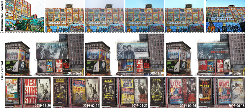
Figure 5: Independent control of illumination effects and time. The top row shows the results of interpolating the illumination embeddings of two real images of 5Pointz, where the leftmost and rightmost images are real images, and all other images are rendered using our method. The bottom rows show the results of rendering scenes across time with fixed illumination embeddings (for Times Square).

4.2 Ablations and Analysis

Qualitative ablation of the step function encoding. An advantage of our method is that it can model abrupt scene-level content changes without overfitting per-image illumination noise. We compare our method with two baselines: (1) ordinary time input without any encoding, and (2) positional encoding of time [34] (with a frequency of 15). We seek to visualize the temporal stability of each method. To do so, given a 4D reconstruction, we first render a video of the scene through time from a fixed viewpoint and with a fixed illumination code (i.e., only content changes). We then compute the mean squared error (MSE) between every two consecutive frames in this video. Plots of MSE over time for each method are shown in Fig. 3. An ideal plot should have large MSE values at sparse points due to abrupt content changes, and zero MSE elsewhere. Our method yields results that exhibit this desired behavior. In contrast, the baseline with no temporal encoding (raw time input) produces smooth transitions across content changes, while positional encoding of time leads to flickering videos. To further illustrate these behaviors, we visualize images around a scene appearance transition point in the first row of Fig. 3.

Quantitative ablations and sensitivity analysis. In addition to view synthesis quality, we also evaluate the temporal stability of synthesized views under a fixed illumination embedding, which indicates the degree of disentanglement between illumination effects and content changes. Similar to the ablations discussed above, we measure temporal stability using the statistics of MSE image differences between each two adjacent frames over time, for videos rendered at a fixed viewpoint with fixed illumination embedding. Specifically, we choose the mean and entropy of these MSE values as our stability metrics. Higher mean values indicate significant changes between adjacent frames, corresponding to temporal flicker. High entropy is associated with high uncertainty in the distribution. Considering image differences over time, high entropy values indicate that scene content changes are distributed throughout time, and are not “peaky”. Smaller mean and entropy values indicate that the changes are more concentrated, indicating better modeling of scene content with discrete and sporadic changes. Please refer to the supplement for additional details on how these metrics are calculated.

We quantitatively ablate our encoding method in terms of view synthesis stability and quality in Tab. 2. We show several baselines and variants: (1) w/o Time which does not take time as input, (2) w/o Encoding, which directly takes raw, unencoded time as input, and (3) Learned Latent, mapping time to a set of learned latent codes. We also change the activation function from ReLU to SIREN [49] and to Gaussian [41], which have been shown to have more powerful modeling abilities. The baselines of positional encoding with different frequencies are also included. While many variants achieve reasonable reconstruction quality, our method can also achieve both low mean and entropy.

We also provide a sensitivity analysis on the dimension of the vector size of the learned step functions (Dim.) in Tab. 2. The results show that our method can achieve high view synthesis quality once the dimension is $\geq 16$. Larger dimensions lead to slightly lower temporal coherence, but not a large degradation. This suggests that we can simply set the number of step functions to a number larger than the number of expected changes in that scene. We set Dim. to 16 in our experiments for all scenes except Times Square, where we set Dim. to 32.

Further qualitative and quantitative ablations of the step function encoding can be found in the supp. material.

Application. We demonstrate the ability of our method to render plausible and photo-realistic images with controlled time and illumination effects in Fig. 5.

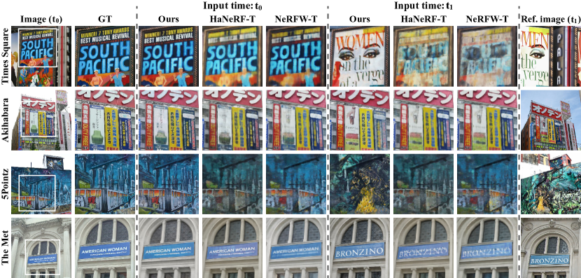
Figure 6: Qualitative comparison with the state of the art. The three column images under Input time: $\text{t}_{x}$ are rendered using timestamps $\text{t}_{x}$ and the viewpoints of the left image. Our method renders high-quality images and produces plausible images when changing the input time.

	4D view synthesis	Times Square				Akihabara				5Pointz				The Met
		Entropy $\downarrow$	PSNR $\uparrow$	SSIM $\uparrow$	LPIPS $\downarrow$	Entropy $\downarrow$	PSNR $\uparrow$	SSIM $\uparrow$	LPIPS $\downarrow$	Entropy $\downarrow$	PSNR $\uparrow$	SSIM $\uparrow$	LPIPS $\downarrow$	Entropy $\downarrow$	PSNR $\uparrow$	SSIM $\uparrow$	LPIPS $\downarrow$
NeRFW [29]	✗	N/A	16.59	0.820	0.211	N/A	17.41	0.853	0.164	N/A	17.52	0.545	0.500	N/A	23.21	0.881	0.159
HaNeRF [6]	✗	N/A	15.39	0.807	0.218	N/A	17.50	0.860	0.160	N/A	16.82	0.539	0.508	N/A	22.32	0.882	0.158
NeRFW-T	✓	4.990	18.71	0.847	0.190	5.483	19.16	0.874	0.140	5.768	19.41	0.611	0.418	4.923	23.83	0.875	0.164
HaNeRF-T	✓	4.929	17.36	0.844	0.189	5.565	18.39	0.873	0.140	5.881	17.90	0.585	0.445	4.943	22.56	0.881	0.156
Ours	✓	3.122	20.87	0.894	0.132	2.482	20.31	0.902	0.101	2.213	21.32	0.745	0.274	2.399	24.07	0.895	0.129

Table 3: Quantitative comparison with the state of the art. We augment NeRF-W and HaNeRF to take time as input (*-T). Our method outperforms prior methods across all metrics, demonstrating that our method can better handle such time-varying Internet collections.

4.3 Comparisons with the State of the Art

We compare to the state-of-the-art methods NeRF-W [29] and HaNeRF [6], which both reconstruct high-fidelity scene models via implicit representations [34]. NeRF-W models illumination using per-image embeddings, while HaNeRF models illumination using a CNN module. However, these methods are designed for static landmarks and cannot handle our test scenes with substantial content changes. We therefore extend these methods by adding time as a network input for fairer comparisons.

We present quantitative and qualitative comparisons with these methods in Tab. 3 and Fig. 6. Our method produces lower entropy across all the scenes. In addition to better temporal stability, our method also has better view synthesis quality. We attribute this to the use of a well-designed appearance parametric encoding. We include ablations of the parametric appearance encoding in the supplemental material. To compare the ability of view synthesis through time, we synthesize photos of the same viewpoint at another time as shown in Fig. 6. The step function encoding helps avoid blending artifacts. In contrast, the other methods often exhibit such artifacts when content changes occur, as is evident in the supplemental video.

5 Conclusion

We explored the problem of chronology reconstruction, aiming to reconstruct and render temporally complex scenes with controlled viewpoint, time, and illumination effects from Internet photos. We proposed a new neural scene representation equipped with a novel step function encoding to address several challenges, including the entanglement of illumination variation and scene content changes, as well as abrupt scene content changes. We also collected a new dataset to benchmark this problem. Experiments show that our method exhibits state-of-the-art performance and is capable of producing plausible, stable view synthesis results across time. Detailed ablations and analysis were conducted to validate our proposed components.

Limitations and future work. Our method takes as input Internet photos with timestamps. Inaccurate timestamps may hinder the training process, and Internet photos that do not have timestamps cannot be utilized for training. Exploring how to simultaneously predict timestamps is an interesting avenue for future work. In addition, some urban scenes such as Times Square have billboards that display videos (not still images), which are difficult for our method to reconstruct, as their content has high temporal frequency is not well supported by other images in the collection.

Acknowledgements. The authors would like to acknowledge support from Information Technology Center and State Key Lab of CAD&CG, Zhejiang University.

In the supplementary material, we present more implementation details, results, and discussion.

Appendix A Method Details

A.1 Data Processing Details

Given Internet photos of a landmark, one way to obtain camera calibration and scene structure is to run COLMAP with built-in acceleration techniques such as Vocabulary Tree Matching and Hierarchical Mapper. However, given the huge number of Internet photos (up to 300K) in our problem, this process requires very high computing resources and up to several TB of memory. To efficiently calibrate 300K images, we design a scheme that can utilize multiple GPU machines in parallel, while solves the problem of computing resources and memory requirements. Specifically, we first randomly divide the pictures into several parts that partially overlap, and then run COLMAP for each part on a GPU separately and in parallel. We then merge these models using the overlapping registered images.

The whole calibrated scene may be too big to reconstruct for the implicit representation. Instead of reconstructing the whole scene, we attempt to reconstruct a piece of the scene. Specifically, given a SFM sparse point cloud of the scene, we can select a interested region from it using MeshLab. Then we can obtain the images, which are registered to the model using the points in the selected interesting region.

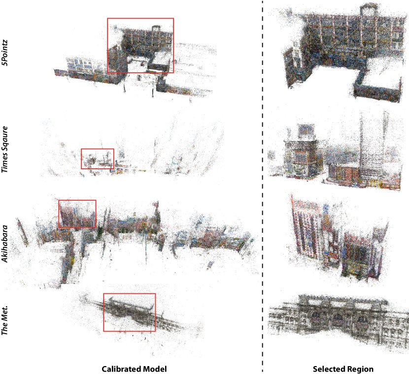
Figure 11: Scene scale visualization. The left column images are the sparse point cloud of the COLMAP model. We select an interesting region from the sparse point cloud using MeshLab.

Please see Fig. 11 for SfM results and our selected regions.

A.2 Sky Modeling

Given an outdoor scene, we can use the SFM sparse point cloud to define the near and far planes for sampling points to optimize our representation. For the sky part, this kind of sampling tends to recover a cloud above the building, causing artifacts when we conduct view synthesis over a large angle range due to wrong geometry. To address the issue, we use a spherical radiance map proposed in [15] to model the sky. Specifically, we map the view direction and the image illumination embedding to the sky color using an MLP and then use alpha blending to obtain the final image color.

A.3 Model Architecture Details

Fig. 12 shows our model architecture. Given a 3D point coordinate $\mathbf{xyz}$ and timestamp, along with an illumination embedding and view direction, we use an MLP to predict its radiance and density. For simplicity, we assume that the scene geometry is mostly constant, and only the appearance changes over time. Therefore, we use an MLP (colored in orange in Fig. 12) to model the geometry and use an MLP (colored in blue in Fig. 12) to model time-varying appearance.

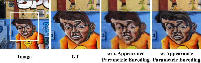
Figure 7: Ablation on the appearance parametric encoding. As illustrated above, using a parametric encoding significantly affects the rendering quality.

A.4 Entropy Details.

Our technical contribution lies in the step function encoding, which enables us to model abrupt scene-level content change without overfitting per-image illumination variation. We use the view synthesis stability (Entropy) along the time to quantify it. Specifically, we first render a video with a fixed viewpoint and a fixed illumination embedding. Then we compute the image difference (MSE) over two consecutive frames of this video to obtain the MSE over time. The distribution of MSE along the time can be regarded as the distribution of content changes over time. The ideal distribution should be concentrated into several points. Given a distribution $P$, which takes values in the alphabet $\mathcal{P}$ and is distributed by $p:\mathcal{P}\rightarrow[0,1]$ (the normalized MSE over time), its entropy $E$ can be computed as:

$$E(P)=\sum_{x_{i}\in\mathcal{P}}-p(x_{i})\text{log\;}p(x_{i}).$$ (9)

When $x$ is equal to zero or one, the function $y=-xlog(x)$ is zero, while this function is positive when $x$ is between zero and one. An ideal concentrated distribution has zero entropy.

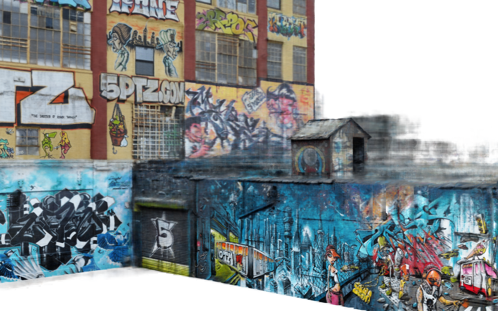
Figure 8: Our method cannot reconstruct blind spots well. People cannot see the top of this small platform when standing on the ground to take pictures.

Appendix B Additional Results

B.1 Ablation on the Step Func. Encoding

To further demonstrate the advantages of step function encoding (in addition to the ablation on the step function encoding we present in the main paper), we carefully selected a train/test split for 5Pointz and evaluated it by visual inspection. This test split contains a large number of images captured at the time of scene content changes. Without using the step function encoding, there would be noticeable blending artifacts in such a test split. Specifically, the results of using step function encoding versus not using it are 19.19/0.715/0.307 and 18.07/0.678/0.345 (PSNR/SSIM/LPIPS), respectively. We present qualitative results on Fig. 10.

B.2 Ablation on the Parametric Encoding

We find that the parametric encoding for appearance modeling significantly affects the rendering quality. Specifically, models with and without proposed parameter encoding produce 19.48/0.612/0.423 and 21.32/0.745/0.274 on 5Pointz in terms of PSNR/SSIM/LPIPS metrics, respectively. We provide a visual ablation on Fig. 7.

B.3 Ablation on the Static-geometry Assumption

We run an ablation study on 5Pointz testing the effect of allowing dynamic geometry, and the results indicate a slight decrease in performance (20.82/0.729 vs. 21.32/0.744 in terms of PSNR/SSIM). Note that all baselines we evaluate assume static geometry, to ensure a fair comparison.

B.4 Scalability of Step Function Encoding

Fig. 9 shows that our method works for synthetic signals with nearly 100 transitions, indicating the scalability of our approach. Specifically, the synthetic signals have multiple dimensions, with each dimension consisting of a randomly segmented and discretized value. Such signals are similar to real-world scenarios, where the value in each dimension can be analogized to a billboard in a real-world scene.

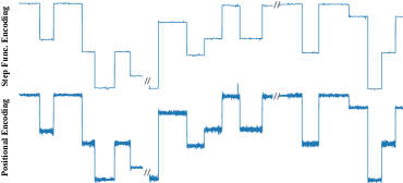
Figure 9: An extension of the experiment in Fig. 3 of main paper. The input noisy signal has 96 transitions, and the dimension of the step function encoding is set to 128. This figure shows fragments of selected transitions. Compared to positional encoding, our method exhibits better temporal stability.

Figure 10: Qualitative ablation on the step function encoding. We focus on the evaluation of manually annotated valid pixels for reasonable metric computation. It can be observed that blending artifacts appear when step function encoding (Step Func.) is not used. This demonstrates the effectiveness of Step Function Encoding.

Appendix C Discussion

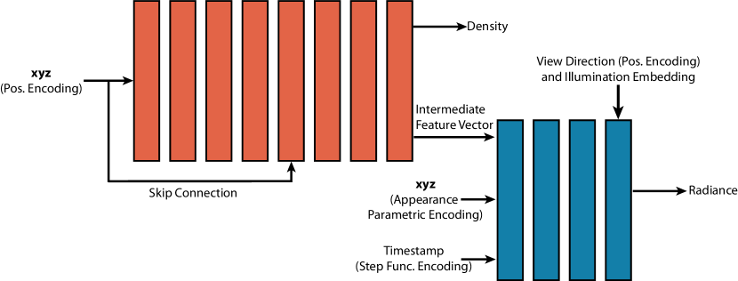
Figure 12: Model Architecture. Step Func. Encoding and Pos. Encoding represent Step Function Encoding and Positional Encoding, respectively. Each layer of the MLP has 256 neurons. We use ReLU as our activation function.

C.1 Time Period Selection

We reconstructed 4 scenes in the period 2009—2013. We chose this period because we found that Flickr was actively used during this period, which provides us with lots of photos. After this period, Flickr became less popular, perhaps due to the emerging social media platforms. For example, Flickr has nearly 80,000 pictures about Akihabara in 2010-2013, but there are less than 10,000 pictures about Akihabara in the last 4 years. Future datasets should also consider these social platforms, if interested in representing more recent years.

C.2 Additional discussion on transient object detection

Why does transient object detection not interfere with our goal to disentangle per-image changes from scene-level changes? The appearance of a scene at a certain stage is usually observed by multiple images, while transient objects are not. Uncertainty loss tends to increase the uncertainty of regions where the model cannot learn (e.g., regions of transient objects), while minimizing uncertainty in other regions. The model can more easily learn scene appearance changes in a 3D coherent way to fit regions with scene appearance changes, rather than predicting these regions with high uncertainty.

C.3 Additional Discussion on Artifacts

In addition to limitations in Sec.5 of the main paper, our method also has the limitation of not being able to reconstruct regions with very few observations. This problem is relatively common for landmark reconstruction from Internet photos. We include some visualization results in Fig. 8.

References

- [1] Sameer Agarwal, Yasutaka Furukawa, Noah Snavely, Ian Simon, Brian Curless, Steven M Seitz, and Richard Szeliski. Building rome in a day. ACM Communications, 2011.
- [2] Boming Zhao and Bangbang Yang, Zhenyang Li, Zuoyue Li, Guofeng Zhang, Jiashu Zhao, Dawei Yin, Zhaopeng Cui, and Hujun Bao. Factorized and controllable neural re-rendering of outdoor scene for photo extrapolation. In ACM MM, 2022.
- [3] Eric R. Chan, Connor Z. Lin, Matthew A. Chan, Koki Nagano, Boxiao Pan, Shalini De Mello, Orazio Gallo, Leonidas Guibas, Jonathan Tremblay, Sameh Khamis, Tero Karras, and Gordon Wetzstein. Efficient geometry-aware 3D generative adversarial networks. In CVPR, 2021.
- [4] Gaurav Chaurasia, Sylvain Duchene, Olga Sorkine-Hornung, and George Drettakis. Depth synthesis and local warps for plausible image-based navigation. ACM TOG, 2013.
- [5] Liang-Chieh Chen, Yukun Zhu, George Papandreou, Florian Schroff, and Hartwig Adam. Encoder-decoder with atrous separable convolution for semantic image segmentation. In ECCV, 2018.
- [6] Xingyu Chen, Qi Zhang, Xiaoyu Li, Yue Chen, Ying Feng, Xuan Wang, and Jue Wang. Hallucinated neural radiance fields in the wild. In CVPR, 2022.
- [7] Abe Davis, Marc Levoy, and Fredo Durand. Unstructured light fields. In Eurographics, 2012.
- [8] Jiemin Fang, Taoran Yi, Xinggang Wang, Lingxi Xie, Xiaopeng Zhang, Wenyu Liu, Matthias Nießner, and Qi Tian. Fast dynamic radiance fields with time-aware neural voxels. SIGGRAPH Asia, 2022.
- [9] John Flynn, Ivan Neulander, James Philbin, and Noah Snavely. Deepstereo: Learning to predict new views from the world’s imagery. In CVPR, June 2016.
- [10] Jan-Michael Frahm, Pierre Fite-Georgel, David Gallup, Tim Johnson, Rahul Raguram, Changchang Wu, Yi-Hung Jen, Enrique Dunn, Brian Clipp, Svetlana Lazebnik, et al. Building rome on a cloudless day. In ECCV, 2010.
- [11] Yasutaka Furukawa, Brian Curless, Steven M Seitz, and Richard Szeliski. Towards internet-scale multi-view stereo. In CVPR, 2010.
- [12] Chen Geng, Sida Peng, Zhen Xu, Hujun Bao, and Xiaowei Zhou. Learning neural volumetric representations of dynamic humans in minutes. In CVPR, 2023.
- [13] Michael Goesele, Noah Snavely, Brian Curless, Hugues Hoppe, and Steven M Seitz. Multi-view stereo for community photo collections. In ICCV, 2007.
- [14] Steven J Gortler, Radek Grzeszczuk, Richard Szeliski, and Michael F Cohen. The lumigraph. In SIGGRAPH, 1996.
- [15] Zekun Hao, Arun Mallya, Serge Belongie, and Ming-Yu Liu. Gancraft: Unsupervised 3d neural rendering of minecraft worlds. In ICCV, 2021.
- [16] Erik Härkönen, Miika Aittala, Tuomas Kynkäänniemi, Samuli Laine, Timo Aila, and Jaakko Lehtinen. Disentangling random and cyclic effects in time-lapse sequences. ACM TOG, 2022.
- [17] Nima Khademi Kalantari, Ting-Chun Wang, and Ravi Ramamoorthi. Learning-based view synthesis for light field cameras. ACM TOG, 2016.
- [18] Marc Levoy and Pat Hanrahan. Light field rendering. In SIGGRAPH, 1996.
- [19] Tianye Li, Mira Slavcheva, Michael Zollhoefer, Simon Green, Christoph Lassner, Changil Kim, Tanner Schmidt, Steven Lovegrove, Michael Goesele, Richard Newcombe, et al. Neural 3d video synthesis from multi-view video. In CVPR, 2022.
- [20] Zhengqi Li, Simon Niklaus, Noah Snavely, and Oliver Wang. Neural scene flow fields for space-time view synthesis of dynamic scenes. In CVPR, 2021.
- [21] Zhengqi Li and Noah Snavely. Learning intrinsic image decomposition from watching the world. In CVPR, 2018.
- [22] Zhengqi Li, Qianqian Wang, Forrester Cole, Richard Tucker, and Noah Snavely. Dynibar: Neural dynamic image-based rendering. In CVPR, 2023.
- [23] Zhengqi Li, Wenqi Xian, Abe Davis, and Noah Snavely. Crowdsampling the plenoptic function. In ECCV, 2020.
- [24] Haotong Lin, Sida Peng, Zhen Xu, Yunzhi Yan, Qing Shuai, Hujun Bao, and Xiaowei Zhou. Efficient neural radiance fields for interactive free-viewpoint video. In SIGGRAPH Asia, 2022.
- [25] Andrew Liu, Shiry Ginosar, Tinghui Zhou, Alexei A Efros, and Noah Snavely. Learning to factorize and relight a city. In European Conference on Computer Vision, pages 544–561. Springer, 2020.
- [26] Lingjie Liu, Jiatao Gu, Kyaw Zaw Lin, Tat-Seng Chua, and Christian Theobalt. Neural sparse voxel fields. NeurIPS, 2020.
- [27] Ricardo Martin-Brualla, David Gallup, and Steven M Seitz. 3d time-lapse reconstruction from internet photos. In ICCV, 2015.
- [28] Ricardo Martin-Brualla, David Gallup, and Steven M Seitz. Time-lapse mining from internet photos. ACM TOG, 2015.
- [29] Ricardo Martin-Brualla, Noha Radwan, Mehdi S. M. Sajjadi, Jonathan T. Barron, Alexey Dosovitskiy, and Daniel Duckworth. NeRF in the Wild: Neural Radiance Fields for Unconstrained Photo Collections. In CVPR, 2021.
- [30] Kevin Matzen and Noah Snavely. Scene chronology. In ECCV, 2014.
- [31] Lars M. Mescheder, Michael Oechsle, Michael Niemeyer, Sebastian Nowozin, and Andreas Geiger. Occupancy networks: Learning 3d reconstruction in function space. In CVPR, 2019.
- [32] Moustafa Meshry, Dan B Goldman, Sameh Khamis, Hugues Hoppe, Rohit Pandey, Noah Snavely, and Ricardo Martin-Brualla. Neural rerendering in the wild. In CVPR, 2019.
- [33] Ben Mildenhall, Pratul P Srinivasan, Rodrigo Ortiz-Cayon, Nima Khademi Kalantari, Ravi Ramamoorthi, Ren Ng, and Abhishek Kar. Local light field fusion: Practical view synthesis with prescriptive sampling guidelines. ACM TOG, 2019.
- [34] Ben Mildenhall, Pratul P. Srinivasan, Matthew Tancik, Jonathan T. Barron, Ravi Ramamoorthi, and Ren Ng. Nerf: Representing scenes as neural radiance fields for view synthesis. In ECCV, 2020.
- [35] Michael Niemeyer, Lars M. Mescheder, Michael Oechsle, and Andreas Geiger. Differentiable volumetric rendering: Learning implicit 3d representations without 3d supervision. In CVPR, 2020.
- [36] Jeong Joon Park, Peter Florence, Julian Straub, Richard A. Newcombe, and Steven Lovegrove. Deepsdf: Learning continuous signed distance functions for shape representation. In CVPR, 2019.
- [37] Keunhong Park, Utkarsh Sinha, Jonathan T. Barron, Sofien Bouaziz, Dan B Goldman, Steven M. Seitz, and Ricardo Martin-Brualla. Nerfies: Deformable neural radiance fields. In ICCV, 2021.
- [38] Keunhong Park, Utkarsh Sinha, Peter Hedman, Jonathan T Barron, Sofien Bouaziz, Dan B Goldman, Ricardo Martin-Brualla, and Steven M Seitz. Hypernerf: A higher-dimensional representation for topologically varying neural radiance fields. arXiv, 2021.
- [39] Sida Peng, Yunzhi Yan, Qing Shuai, Hujun Bao, and Xiaowei Zhou. Representing volumetric videos as dynamic mlp maps. In CVPR, 2023.
- [40] Albert Pumarola, Enric Corona, Gerard Pons-Moll, and Francesc Moreno-Noguer. D-nerf: Neural radiance fields for dynamic scenes. In CVPR, 2021.
- [41] Sameera Ramasinghe and Simon Lucey. Beyond periodicity: Towards a unifying framework for activations in coordinate-mlps. In ECCV, 2022.
- [42] Viktor Rudnev, Mohamed Elgharib, William Smith, Lingjie Liu, Vladislav Golyanik, and Christian Theobalt. Nerf for outdoor scene relighting. In ECCV, 2022.
- [43] Sara Fridovich-Keil and Giacomo Meanti, Frederik Rahbæk Warburg, Benjamin Recht, and Angjoo Kanazawa. K-planes: Explicit radiance fields in space, time, and appearance. In CVPR, 2023.
- [44] Frederik Schaffalitzky and Andrew Zisserman. Multi-view matching for unordered image sets, or “how do i organize my holiday snaps?”. In ECCV, 2002.
- [45] Grant Schindler and Frank Dellaert. Probabilistic temporal inference on reconstructed 3d scenes. In CVPR, 2010.
- [46] Johannes L Schonberger and Jan-Michael Frahm. Structure-from-motion revisited. In CVPR, 2016.
- [47] Johannes L Schönberger, Enliang Zheng, Jan-Michael Frahm, and Marc Pollefeys. Pixelwise view selection for unstructured multi-view stereo. In ECCV, 2016.
- [48] Shuhan Shen. Accurate multiple view 3d reconstruction using patch-based stereo for large-scale scenes. TIP, 2013.
- [49] Vincent Sitzmann, Julien Martel, Alexander Bergman, David Lindell, and Gordon Wetzstein. Implicit neural representations with periodic activation functions. NeurIPS, 2020.
- [50] Vincent Sitzmann, Justus Thies, Felix Heide, Matthias Nießner, Gordon Wetzstein, and Michael Zollhöfer. Deepvoxels: Learning persistent 3d feature embeddings. In CVPR, 2019.
- [51] Noah Snavely, Steven M Seitz, and Richard Szeliski. Photo tourism: exploring photo collections in 3d. In SIGGRAPH, 2006.
- [52] Noah Snavely, Steven M Seitz, and Richard Szeliski. Modeling the world from internet photo collections. IJCV, 2008.
- [53] Jiaming Sun, Xi Chen, Qianqian Wang, Zhengqi Li, Hadar Averbuch-Elor, Xiaowei Zhou, and Noah Snavely. Neural 3D reconstruction in the wild. In SIGGRAPH, 2022.
- [54] Kalyan Sunkavalli, Wojciech Matusik, Hanspeter Pfister, and Szymon Rusinkiewicz. Factored time-lapse video. In ACM SIGGRAPH, pages 101–es. 2007.
- [55] Richard Tucker and Noah Snavely. Single-view view synthesis with multiplane images. In Proceedings of the IEEE/CVF Conference on Computer Vision and Pattern Recognition, pages 551–560, 2020.
- [56] Chaoyang Wang, Ben Eckart, Simon Lucey, and Orazio Gallo. Neural trajectory fields for dynamic novel view synthesis. arXiv, 2021.
- [57] Suttisak Wizadwongsa, Pakkapon Phongthawee, Jiraphon Yenphraphai, and Supasorn Suwajanakorn. Nex: Real-time view synthesis with neural basis expansion. In CVPR, 2021.
- [58] Wenqi Xian, Jia-Bin Huang, Johannes Kopf, and Changil Kim. Space-time neural irradiance fields for free-viewpoint video. In CVPR, 2021.
- [59] Jiakai Zhang, Xinhang Liu, Xinyi Ye, Fuqiang Zhao, Yanshun Zhang, Minye Wu, Yingliang Zhang, Lan Xu, and Jingyi Yu. Editable free-viewpoint video using a layered neural representation. ACM TOG, 2021.
- [60] C Lawrence Zitnick, Sing Bing Kang, Matthew Uyttendaele, Simon Winder, and Richard Szeliski. High-quality video view interpolation using a layered representation. ACM TOG, 2004.