Abstract

We develop an algorithm for automatic differentiation of Metropolis-Hastings samplers, allowing us to differentiate through probabilistic inference, even if the model has discrete components within it. Our approach fuses recent advances in stochastic automatic differentiation with traditional Markov chain coupling schemes, providing an unbiased and low-variance gradient estimator. This allows us to apply gradient-based optimization to objectives expressed as expectations over intractable target densities. We demonstrate our approach by finding an ambiguous observation in a Gaussian mixture model and by maximizing the specific heat in an Ising model.

1 Introduction

Metropolis-Hastings (MH) samplers have found wide applicability across a number of disciplines due to their ability to sample from distributions with intractable normalizing constants. However, MH samplers are not traditionally differentiable due to the presence of discrete accept/reject steps for proposed samples Zhang et al. (2021). This poses a problem when we wish to optimize objectives that are themselves a function of the sampler’s output.

In this work, we propose an approach for unbiasedly differentiating a MH sampler. Specifically, consider a family of distributions $\mu_{\theta}$ dependent on a parameter $\theta$, targeted by a MH sampler $\{Z_{t}^{\theta}\}_{t=1}^{\infty}$. The samples can be used to approximate expectations of functions $f$ with respect to $\mu_{\theta}$; that is, if the sampler is ergodic Maruyama & Tanaka (1959),

$$\mathop{\mathbb{E}}_{X^{\theta}\sim\mu_{\theta}}\left[f\left(X^{\theta}\right)\right]=\lim_{T\to\infty}\frac{1}{T}\sum_{t=1}^{T}f\left(Z_{t}^{\theta}\right),$$ (1)

for bounded and measurable $f$. Now, consider optimizing some function of $\mu_{\theta}$. For instance, Chandra et al. (2022) consider Bayesian inference on probabilistic models of human cognition, seeking an observation $\theta$ which maximizes the variance of the posterior $\mathrm{P}(x\mathbin{|}{}\theta)$ of a latent $x$. In such a case, we may be interested in estimating the gradient of an expectation over the density:

$$\frac{\partial}{\partial\theta}\mathop{\mathbb{E}}_{X^{\theta}\sim\mu_{\theta}}\left[f\left(X^{\theta}\right)\right].$$ (2)

This is challenging when $\mu_{\theta}$ can only be sampled by Monte Carlo methods. One approach to estimating (2) is to differentiate through the sampling process itself. However, direct application of gradient estimation strategies such as the score function estimator to MH leads to high variance as the chain length increases Thin et al. (2021); Doucet et al. (2023). Our key insight is that we can form a consistent estimator as the MH chain length increases, by coupling two MH chains with perturbed targets.

Prior work has considered sampling procedures that avoid MH accept/reject steps (Zhang et al., 2021; Doucet et al., 2022; 2023) or differentiated only through the continuous dynamics of samplers such as Hamiltonian Monte Carlo Chandra et al. (2022); Campbell et al. (2021); Zoltowski et al. (2021). The latter approach leads to biased gradients and does not apply to discrete target distributions. In this work, we instead unbiasedly differentiate the accept/reject steps. We make the following contributions:

• A provably unbiased algorithm for differentiating through MH with $\mathcal{O}(1)$ multiplicative computational overhead, that applies to arbitrary discrete or continuous target distributions, based on smoothed perturbation analysis Fu et al. (1997) and stochastic automatic differentiation Arya et al. (2022).

• A demonstration of how Monte Carlo coupling schemes Wang et al. (2021); Propp & Wilson (1996) may be applied to produce an efficient low-variance single-chain MH gradient estimator.

• Empirical verifications of the correctness of our gradient estimator and preliminary applications to optimizing the posterior of a Gaussian mixture model and the specific heat of an Ising model.

2 Differentiable Metropolis-Hastings

Consider the use of MH to sample from a target distribution $\mu_{\theta}$ using an unnormalized density $g_{\theta}(x)\propto\mu_{\theta}(x)$ and a proposal density $q(x^{\prime}\mathbin{|}{}x)$. At state $x=Z_{t}^{\theta}$, we draw a candidate sample $x^{\prime}\sim q(\cdot\mathbin{|}{}x)$ and accept it with probability

$$\alpha_{\theta}(x^{\prime}\mathbin{|}{}x)=\min\left(1,\frac{g_{\theta}(x^{\prime})}{g_{\theta}(x)}\frac{q(x\mathbin{|}{}x^{\prime})}{q(x^{\prime}\mathbin{|}{}x)}\right).$$ (3)

Algorithm 1 shows the corresponding algorithm.

1:  Input: functions $g_{\theta},f$, proposal $q$, start state $x_{1}$

2:  $S:=x_{1}$

3:  for $i=1$ to $T-1$ do

4:     sample $x^{\prime}\sim q(\cdot\mathbin{|}{}x_{i})$, $U\sim\operatorname{Unif}()$

5:     $b:=U\leq\alpha_{\theta}(x^{\prime}\mathbin{|}x_{i})$

6:     if $b=1$ then $x_{i+1}:=x^{\prime}$ else $x_{i+1}:=x_{i}$ end if

7:     $S:=S+f(x_{i+1})$

8:  end for

9:  return $S/T$

Algorithm 1 $T$-sample Metropolis-Hastings

Now, let us understand the sensitivity of MH with respect to a parameter $\theta\in\mathbb{R}$. The acceptance probability $\alpha_{\theta}(x^{\prime}\mathbin{|}{}x)$ depends on $\theta$, with derivative in the non-trivial case

$$\frac{\partial}{\partial\theta}\alpha_{\theta}(x^{\prime}\mathbin{|}{}x)=\alpha_{\theta}(x^{\prime}\mathbin{|}{}x)\frac{\partial}{\partial\theta}\log\frac{g_{\theta}(x^{\prime})}{g_{\theta}(x)}.$$ (4)

This acceptance probability feeds into the discrete random accept/reject step (Algorithm 1, lines 4-5). A number of gradient estimation approaches have been developed in such a discrete random setting, including score-function estimators Kleijnen & Rubinstein (1996), measure-valued derivatives Heidergott & Vázquez-Abad (2008), and smoothed perturbation analysis (SPA) Fu et al. (1997). In this work, we opt for an SPA-based estimator, which for a purely discrete random variable $X^{\theta}$ assumes the following form Heidergott & Vázquez-Abad (2008); Arya et al. (2022):

$$\frac{\partial}{\partial\theta}\mathbb{E}[f(X^{\theta})]=\mathbb{E}\left[w^{\theta}\left(f(Y^{\theta})-f(X^{\theta})\right)\right].$$ (5)

Intuitively, the estimator works by taking differences between the program evaluated at the primal sample $X^{\theta}$ and at a discretely perturbed alternative sample $Y^{\theta}$ that “branches off” the primal, weighting these by a possibly random $w^{\theta}$ related to the infinitesimal probability of a change. In the case of the long Markov chains produced by MH, we will see that the coupling of $X^{\theta}$ and $Y^{\theta}$, i.e. the form of their joint distribution, plays a key role in reducing variance.

There has been recent interest in automating the application of such strategies across whole programs Lew et al. (2023); Arya et al. (2022); Krieken et al. (2021). In particular, Arya et al. (2022) develop composition rules for an SPA-based estimator to perform automatic unbiased gradient estimation for discrete random programs, calling their construction “stochastic derivatives.” We use it to develop a differentiable MH sampler, given in Algorithm 2.

Algorithm 2 $T$-sample Differentiable Metropolis-Hastings

1:  Input: functions $g_{\theta},f$, proposal $q$, start state $x_{1}$,

2:            coupled proposal $q_{xy}$

3:  $\partial S:=0$, $y_{1}:=x_{1}$, $w_{1}:=0$

4:  for $i=1$ to $T-1$ do

5:      // Perform MH step for primal and alternative

6:     sample $x^{\prime},y^{\prime}\sim q_{xy}(\cdot,\cdot\mathbin{|}{}x_{i},y_{i})$, $U\sim\operatorname{Unif}()$

7:     $b_{x}:=U\leq\alpha_{\theta}(x^{\prime}\mathbin{|}x_{i})$, $b_{y}:=U\leq\alpha_{\theta}(y^{\prime}\mathbin{|}y_{i})$,

8:     if $b_{x}=1$ then $x_{i+1}:=x^{\prime}$ else $x_{i+1}=x_{i}$ end if

9:     if $b_{y}=1$ then $y_{i+1}:=y^{\prime}$ else $y_{i+1}:=y_{i}$ end if

10:      // Compute stochastic derivative weight

11:     if $b_{x}=1$ then

12:        $w:={\alpha_{\theta}(x^{\prime}\mathbin{|}x_{i})}^{-1}\max(0,-\frac{\partial\alpha_{\theta}(x^{\prime}\mathbin{|}x_{i})}{\partial\theta})$

13:     else

14:        $w:={(1-\alpha_{\theta}(x^{\prime}\mathbin{|}x_{i}))}^{-1}\max(0,\frac{\partial\alpha_{\theta}(x^{\prime}\mathbin{|}x_{i})}{\partial\theta})$

15:     end if

16:      // Prune between previous alternative and new

17:     if $y_{i+1}=x_{i+1}$ then $w_{i}:=0$ end if // drop recoupled

18:     $w_{i+1}:=w+w_{i}$

19:     sample $\varpi\sim\operatorname{Unif}()$

20:     if $\varpi\cdot w_{i+1}<w$ then

21:        if $b_{x}=1$ then $y_{i+1}:=x_{i}$ else $y_{i+1}=x^{\prime}$ end if

22:     end if

23:      // Update derivative estimate

24:     $\partial S:=\partial S+w_{i+1}(f(y_{i+1})-f(x_{i+1}))$

25:  end for

26:  return $\partial S/T$

Most parts of Algorithm 2 follow from directly applying the composition rules of Arya et al. (2022) to Algorithm 1. At a high level, alternative MH samples $y_{i}$ are propagated in parallel to the primal samples $x_{i}$ (lines 6–9). For each primal accept/reject step $b_{x}$, we compute the weight of a flip in $b_{x}$ according to the stochastic derivative estimator (lines 11–15). We employ the pruning strategy given in Arya et al. (2022) to stochastically select a single alternative between the currently tracked alternative and the new possible alternative (lines 17–22), with the extra optimization that we stop tracking alternatives that have recoupled, as they will stay coupled for all future steps and no longer contribute to the derivative. On recoupling, we can thus always prune and consider a new alternative. Note that Algorithm 2 accepts a “coupled proposal” $q_{xy}$, which specifies the joint proposal distribution for the primal and alternative MH chains (line 6). As long as $q_{xy}$ is a valid coupling, Algorithm 2 computes an unbiased derivative estimate of finite-sample MH expectations:

Theorem 2.1.

Suppose that for all $x,y$, it holds that if $x^{\prime},y^{\prime}\sim q_{xy}(\cdot,\cdot\mathbin{|}{}x,y)$ then $x^{\prime}\sim q(\cdot\mathbin{|}{}x)$ and $y^{\prime}\sim q(\cdot\mathbin{|}{}y)$ (i.e. $q_{xy}$ is a proposal coupling), and furthermore that if $x=y$ then $x^{\prime}=y^{\prime}$. Then, with inputs $g_{\theta}(x)\propto\mu_{\theta}(x)$, a bounded and measurable $f$, $q$, $x_{0}$, and $q_{xy}$, the output of Algorithm 2 is an unbiased estimator of

$$\frac{\partial}{\partial\theta}\left(\mathbb{E}\left[\frac{1}{T}\sum_{i=1}^{T}f\left(Z_{t}^{\theta}\right)\right]\right),$$ (6)

where $Z_{t}^{\theta}$ is a MH sampler of $\mu_{\theta}$ with proposal $q$, initial state $Z_{0}^{\theta}=x_{0}$.

While unbiasedness is guaranteed by Theorem 2.1, the choice of coupling is important for the variance performance of Algorithm 2. A simple choice is common random numbers (CRN) Glasserman & Yao (1992), equivalent to using the same random seed for both chains: we use CRN for the accept/reject step in Algorithm 2. For the proposal, we leverage prior work on coupling for its more traditional use: minimizing recoupling time. That is, if alternative trajectories rapidly recouple to the primal, we will be able to consider additional alternative trajectories over the lifetime of the chain, hence reducing variance. Wang et al. (2021) present several schemes for coupling MH proposals. Figure 1 gives an example of the maximal reflection coupling for a Gaussian proposal applied in Algorithm 2: we see that the alternative trajectories recouple within $\approx 5$ steps.

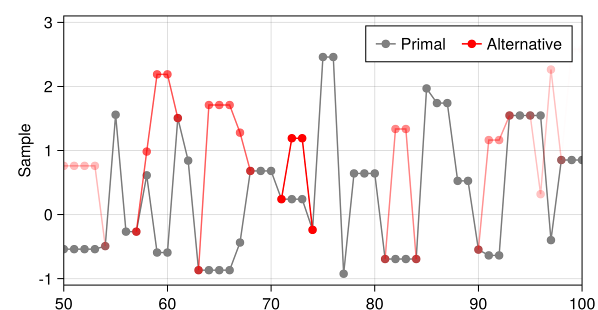
Figure 1: Differentiable MH (Algorithm 2) samples two coupled chains: the primal chain (grey) and a chain containing alternative samples (red), which together allow to estimate the derivative of the sampler. Here we target $\mu_{\theta}\sim\mathcal{N}(\theta,1)$ with $\theta=0.5$ and a maximal reflection proposal coupling. The alpha values of the depicted alternative paths correspond to their weight.

Ultimately, we note that Algorithm 2 can be derived automatically from Algorithm 1 and need not be handwritten; in code, we can implement our differentiable MH by applying StochasticAD.jl of Arya et al. (2022) to Algorithm 1. Only the proposal coupling needs to be manually specified, if it differs from CRN.

3 Examples

3.1 Finding ambiguous observations in a Gaussian mixture model

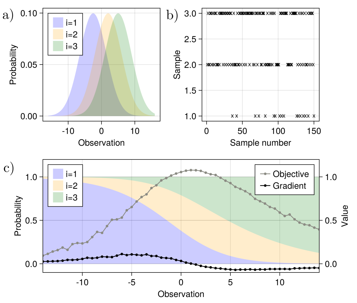
Figure 2: Finding ambiguous observations in a Gaussian mixture model by differentiating MH inference. a) Density of each Gaussian component. b) Samples from an MH chain inferring the component $J$ for the observation $H=4.0$. c) Posterior density of $J$ for each observation. The values of the optimization objective (posterior entropy) and its estimated gradient are overlayed.

Consider a mixture model with three independent Gaussians $N_{i}\sim N(\mu_{i},\sigma)$ with means $\mu_{1}=-2.5,\mu_{2}=2,\mu_{3}=5$, and $\sigma=4$ [Figure 2a)]. Suppose we pick a component $J\in\{1,2,3\}$ uniformly at random and sample $H\sim N_{J}$. Now, conditional on the observation $H$, e.g. the height of a person in a population, we would like to infer the source cluster $J$. By Bayes’ rule, the posterior [Figure 2c)] is

$$\mathrm{P}(J=j\mathbin{|}{}H=h)\propto\mathrm{P}(H=h\mathbin{|}{}J=j)\mathrm{P}(J=j).$$ (7)

In this case, the posterior has a small finite support, allowing us to compute the usually intractable normalization constant of (7) via explicit enumeration. However, in order to test our approach, we consider sampling the posterior by MH (Figure 2b) using only the unnormalized density (7).

Now, we use differentiable MH to optimize the posterior distribution. We seek to find the observation $h$ that maximizes inference ambiguity, i.e. finds the observation for which it is most difficult to determine which cluster it came from by maximizing posterior entropy. Even in this toy setting, a naïve application of the score function estimator yields an estimator whose variance does not decrease with more MH samples (Section A.1). However, Algorithm 2, using maximal independent proposal coupling Vaserstein (1969), does better. This coupling seeks to maximize the probability that the proposals agree and recouple on the next step. A sweep of the objective and its gradient, computed by differentiable MH, is depicted in Figure 2c. Optimization via gradient descent converges to the optimum observation in $\approx 100$ iterations.

3.2 Maximizing the specific heat in an Ising model

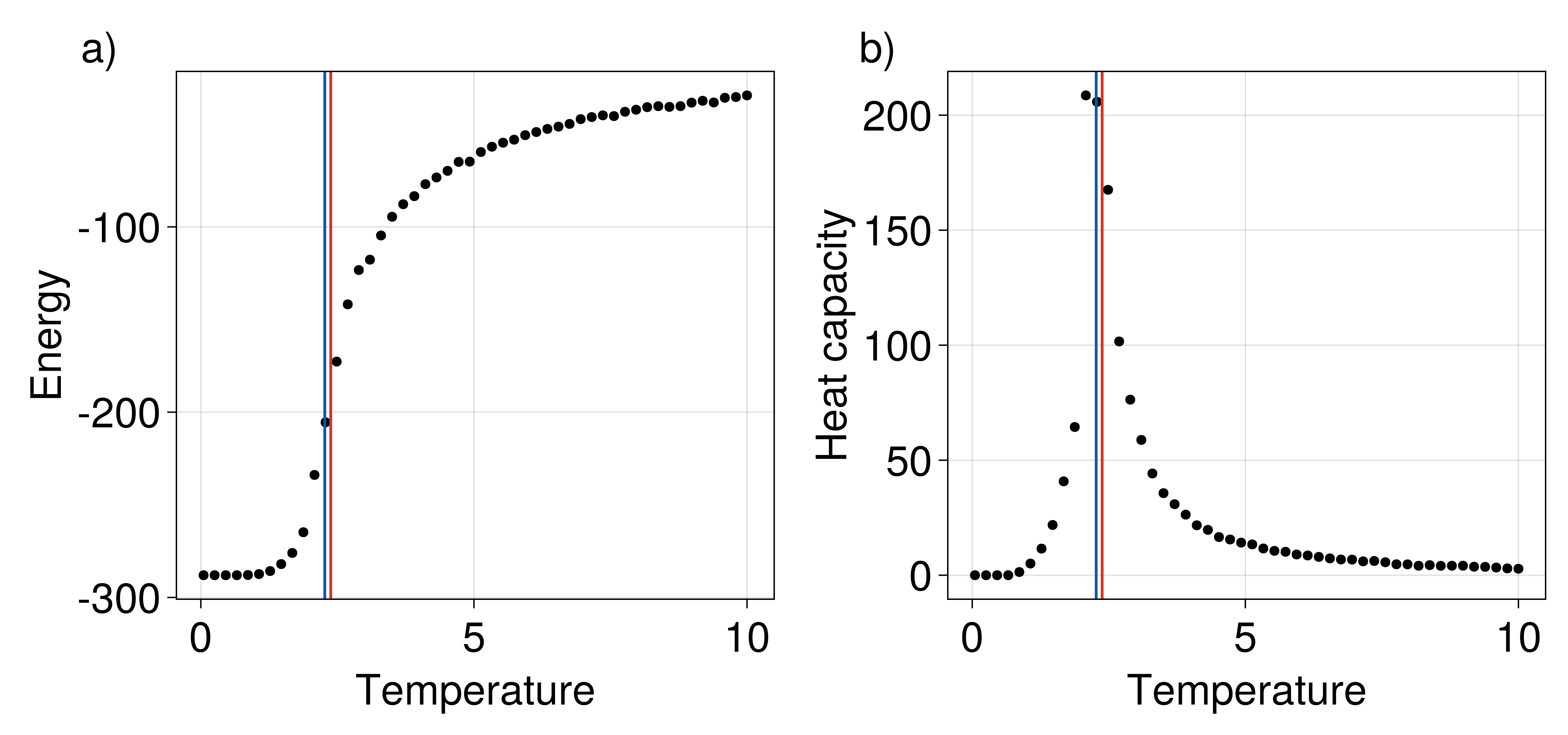
Figure 3: Maximizing the specific heat in an Ising model as a function of temperature $T$ via differentiable MH, for $L=12$ and $\theta=1$. a) Average energy $\mathop{\mathbb{E}}\left[H(X^{T},\theta)\right]$. b) Heat capacity (11). The blue and red lines correspond to the analytical value (10) and the numerically optimized prediction of the critical temperature, respectively.

Next, we consider an example from physics. The random configuration $X^{T}$ of a classical physical system at thermal equilibrium in contact with a large thermal reservoir of temperature $T$, follows the Boltzmann distribution,

$$\mathrm{P}(X^{T}=x\mathbin{|}{}\theta)=e^{-{H}({x},\theta)/(k_{B}T)}/Z(\theta),$$ (8)

where $Z(\theta)=\sum_{x}e^{-{H}({x},\theta)/(k_{B}T)}$ is the partition function. Consider the two-dimensional isotropic Ising model for spin configurations on an $L{\times}L$ square lattice with periodic boundary conditions. The spin $x_{j,k}$ at a site $(j,k)$ can take a value of either $+1$ or $-1$, resulting in a state space of size $2^{L^{2}}$. The Hamiltonian for this model is given by

$$\textstyle H(x,\theta)=-\theta\sum_{j,k=1}^{L}\left(x_{j,k}x_{j,k+1}+x_{j+1,k}x_{j,k}\right),$$ (9)

where the parameter $\theta$ represents the strength of the nearest-neighbor interaction. The identification of phase transitions is central to understanding the properties and behavior of a wide range of material systems Arnold & Schäfer (2022). The Ising model exhibits a symmetry-breaking phase transition at a critical temperature of

$$T_{c}={2\theta}/({k_{B}\log(1+\sqrt{2})}),$$ (10)

in the limit $L\rightarrow\infty$, between an ordered (low temperature) and a disordered (high temperature) phase. This phase transition is associated with a peak in the heat capacity

$$C(T)=\mathop{\operatorname{Var}}\!\left(H(X^{T},\theta)\right)/(k_{B}T^{2}).$$ (11)

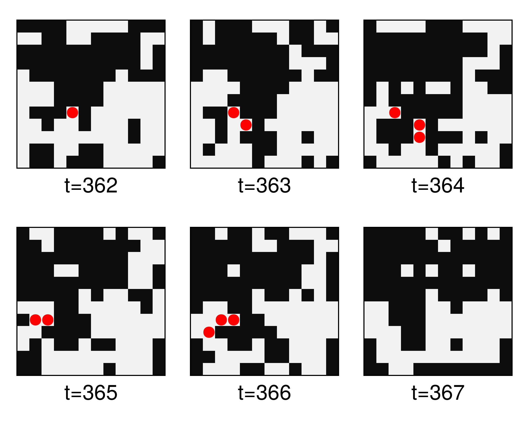
Figure 4: Recoupling of primal (black and white) and alternative (flipped cells in red) spin states in the Ising model over a subrange of sweeps in the heat bath algorithm, with $L=12$.

Our goal is to find the critical temperature by maximizing the heat capacity. In general, computing $C(T)$ by exhaustive enumeration is not feasible due to the size of the configuration space, but it can be computed with a Monte Carlo procedure. To sample configurations we use a variant of the heat bath algorithm in which we pick a site, propose to set the spin at that site to $+1$ or $-1$ with equal probability and use a MH step to decide whether to accept this proposal. We couple by proposing the same change for primal and alternative together with common random numbers to check for acceptance in both chains. It is easy to see that this creates a monotone coupling (Propp & Wilson, 1996). As the primal and alternative at the time of a branch are ordered with respect to the natural partial order on the configuration space, this order is preserved until the branches recouple after a finite time (Figure 4). Having a differentiable MH sampler for $C(T)$, we can then perform stochastic gradient ascent to find the optimal value of $T$, as shown in Figure 3 (optimization trace provided in Section A.3).

4 Conclusion and outlook

We have presented an efficient low-variance derivative estimator for Metropolis-Hastings samplers and showed its efficacy in discrete and high-dimensional spaces. A key avenue for future work is to apply our scheme in settings with many trainable parameters, for example optimizing over models conditioned on observed images and videos (Chandra et al., 2022; 2023), training energy-based models (Du et al., 2020), and working with nested models (Zhang & Amin, 2022). This may require incorporating reverse-mode automatic differentiation and exploring further variance reduction techniques. We may also wish to unbiasedly differentiate samplers with both discrete and continuous dynamics, see e.g. concurrent work on differentiating piecewise deterministic Monte Carlo samplers Seyer (2023). Additionally, for applications such as gradient-based hyperparameter optimization (Campbell et al., 2021), we may also want to differentiate with respect to parameters of the proposal and support alternative optimization objectives such as autocorrelations of the MH chain.

Appendix A Appendix

A.1 Differentiable Metropolis-Hastings via Score Method

Algorithm 3 $T$-sample Differentiable Metropolis-Hastings via Score

1:  Input: functions $g_{\theta},f$, proposal $q$, start state $x_{1}$

2:  $\partial S:=0$, $w:=0$

3:  for $i=1$ to $T-1$ do

4:     sample $x^{\prime}\sim q(\cdot\mathbin{|}{}x_{i})$, $U\sim\operatorname{Unif}()$

5:     $b:=U\leq\alpha_{\theta}(x^{\prime}\mathbin{|}x_{i})$

6:     if $b=1$ then $x_{i+1}:=x^{\prime}$ else $x_{i+1}:=x_{i}$ end if

7:     $w:=w+\dfrac{\partial\log\alpha_{\theta}(x_{i+1}\mathbin{|}x_{i})}{\partial\theta}$

8:     $\partial S:=\partial S+w\cdot f(x_{i+1})$

9:  end for

10:  return $\partial S/T$

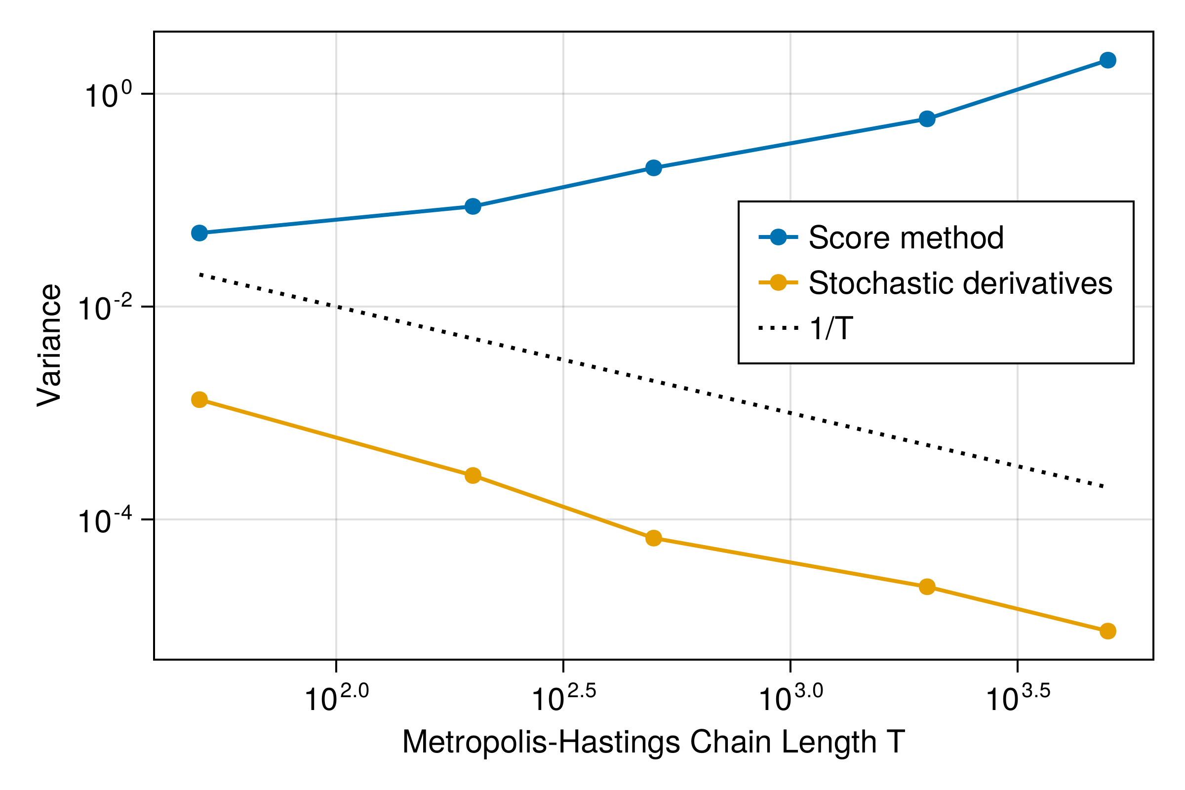
Figure 5: Variance comparison of stochastic derivative-based differentiable MH (Algorithm 2) and score method-based differentiable MH (Algorithm 3), for the Gaussian mixture inference task given in Section 3.1 with the observation $H=0.4$.

Algorithm 3 applies a score-function estimator to each accept/reject step of Algorithm 1. Note that we cannot apply the score-function estimator directly to the density $\mu_{\theta}$, since the normalizing constant is unknown and dependent on the parameter $\theta$. Thus, just as we did with the stochastic derivative estimator in Algorithm 2, we apply the score function estimator to each step of Algorithm 1 to obtain an unbiased estimator of finite-sample expectations for comparison.

A.2 Proof of Theorem 2.1

Proof.

Since Algorithm 1 implements MH, and Algorithm 2 follows from applying the composition rules of Arya et al. (2022) to each step of Algorithm 1, and then applying (5) to compute $\partial S$, the result follows from Theorem 2.6 (Chain Rule) and Proposition 2.3 (Unbiasedness) of Arya et al. (2022). One additional trick employed by Algorithm 2 is to drop the currently tracked alternative if it has recoupled (line 17), which is justified by the assumption that $x=y$ implies $x^{\prime}=y^{\prime}$ and the fact that for the common random numbers coupling $\alpha(y^{\prime}\mathbin{|}y)=\alpha(x^{\prime}\mathbin{|}x)$ implies $b_{x}=b_{y}$, so that chains that recouple are guaranteed to remain coupled and have no further derivative contribution in Equation 5. ∎

A.3 Optimization of the heat capacity in the Ising model

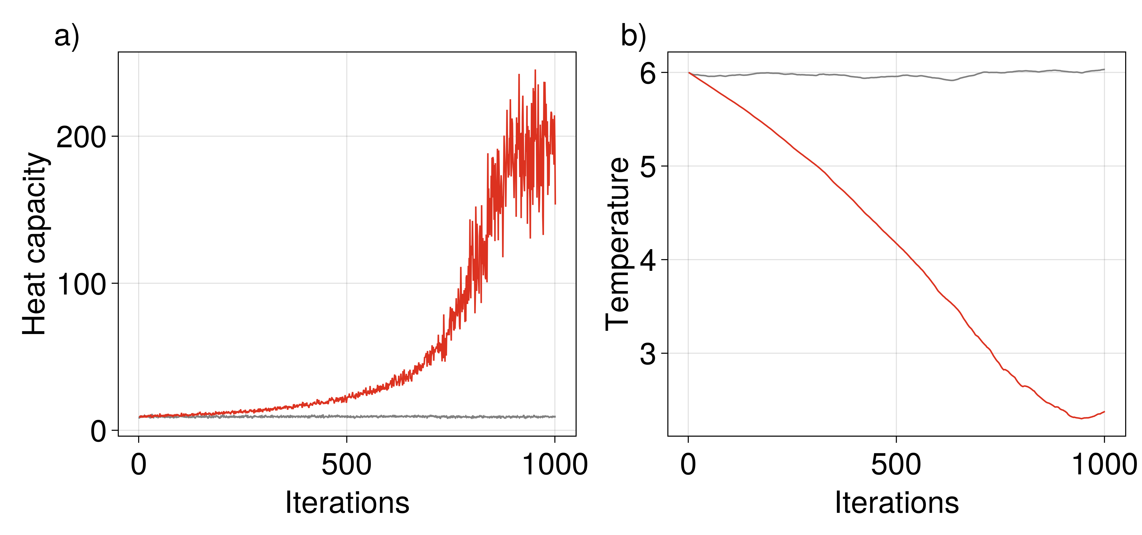
Figure 6: Maximizing the specific heat in an Ising model (9) with respect to temperature $T$ via differentiable MH, for $L=12$ and $\theta=1$. a) Heat capacity (11) across Adam optimizer iterations. b) Temperature across Adam optimizer iterations. The red and gray lines correspond to coupled and uncoupled proposals in Algorithm 2, respectively.

A.4 Code

Code for reproducing the experiments in this paper is available at https://github.com/gaurav-arya/differentiable_mh.

References

- Arnold & Schäfer (2022) Arnold, J. and Schäfer, F. Replacing neural networks by optimal analytical predictors for the detection of phase transitions. Phys. Rev. X, 12:031044, Sep 2022. doi: 10.1103/PhysRevX.12.031044. URL https://link.aps.org/doi/10.1103/PhysRevX.12.031044.
- Arya et al. (2022) Arya, G., Schauer, M., Schäfer, F., and Rackauckas, C. Automatic differentiation of programs with discrete randomness. Advances in Neural Information Processing Systems, 35:10435–10447, 2022.
- Campbell et al. (2021) Campbell, A., Chen, W., Stimper, V., Hernandez-Lobato, J. M., and Zhang, Y. A gradient based strategy for Hamiltonian Monte Carlo hyperparameter optimization. In International Conference on Machine Learning, pp. 1238–1248. PMLR, 2021.
- Chandra et al. (2022) Chandra, K., Li, T.-M., Tenenbaum, J., and Ragan-Kelley, J. Designing perceptual puzzles by differentiating probabilistic programs. In ACM SIGGRAPH 2022 Conference Proceedings, pp. 1–9, 2022.
- Chandra et al. (2023) Chandra, K., Li, T.-M., Tenenbaum, J., and Ragan-Kelley, J. Acting as inverse inverse planning. In Special Interest Group on Computer Graphics and Interactive Techniques Conference Proceedings (SIGGRAPH ’23 Conference Proceedings), August 2023. doi: 10.1145/3588432.3591510.
- Doucet et al. (2022) Doucet, A., Grathwohl, W., Matthews, A. G., and Strathmann, H. Score-based diffusion meets annealed importance sampling. Advances in Neural Information Processing Systems, 35:21482–21494, 2022.
- Doucet et al. (2023) Doucet, A., Moulines, E., and Thin, A. Differentiable samplers for deep latent variable models. Philosophical Transactions of the Royal Society A, 381(2247):20220147, 2023.
- Du et al. (2020) Du, Y., Li, S., Tenenbaum, J., and Mordatch, I. Improved contrastive divergence training of energy based models. arXiv preprint arXiv:2012.01316, 2020.
- Fu et al. (1997) Fu, M., Hu, J.-Q., Fu, M., and Hu, J.-Q. Conditional Monte Carlo gradient estimation. Conditional Monte Carlo: Gradient Estimation and Optimization Applications, 1997.
- Glasserman & Yao (1992) Glasserman, P. and Yao, D. D. Some guidelines and guarantees for common random numbers. Management Science, 38(6):884–908, 1992.
- Heidergott & Vázquez-Abad (2008) Heidergott, B. and Vázquez-Abad, F. Measure-valued differentiation for Markov chains. Journal of Optimization Theory and Applications, 136(2):187–209, 2008.
- Kleijnen & Rubinstein (1996) Kleijnen, J. P. and Rubinstein, R. Y. Optimization and sensitivity analysis of computer simulation models by the score function method. European Journal of Operational Research, 88(3):413–427, 1996.
- Krieken et al. (2021) Krieken, E., Tomczak, J., and Ten Teije, A. Storchastic: A framework for general stochastic automatic differentiation. Advances in Neural Information Processing Systems, 34:7574–7587, 2021.
- Lew et al. (2023) Lew, A. K., Huot, M., Staton, S., and Mansinghka, V. K. ADEV: Sound automatic differentiation of expected values of probabilistic programs. Proceedings of the ACM on Programming Languages, 7(POPL):121–153, 2023.
- Maruyama & Tanaka (1959) Maruyama, G. and Tanaka, H. Ergodic prorerty of n-dimensional recurrent Markov processes. Memoirs of the Faculty of Science, Kyushu University. Series A, Mathematics, 13(2):157–172, 1959.
- Propp & Wilson (1996) Propp, J. G. and Wilson, D. B. Exact sampling with coupled Markov chains and applications to statistical mechanics. Random Structures and Algorithms, 9(1):223–252, 1996.
- Seyer (2023) Seyer, R. Differentiable Monte Carlo samplers with piecewise deterministic Markov processes. Master’s thesis, Chalmers University of Technology & University of Gothenburg, 2023.
- Thin et al. (2021) Thin, A., Kotelevskii, N., Doucet, A., Durmus, A., Moulines, E., and Panov, M. Monte carlo variational auto-encoders. In International Conference on Machine Learning, pp. 10247–10257. PMLR, 2021.
- Vaserstein (1969) Vaserstein, L. N. Markov processes over denumerable products of spaces, describing large systems of automata. Problemy Peredachi Informatsii, 5(3):64–72, 1969.
- Wang et al. (2021) Wang, G., O’Leary, J., and Jacob, P. Maximal couplings of the Metropolis-Hastings algorithm. In International Conference on Artificial Intelligence and Statistics, pp. 1225–1233. PMLR, 2021.
- Zhang et al. (2021) Zhang, G., Hsu, K., Li, J., Finn, C., and Grosse, R. B. Differentiable annealed importance sampling and the perils of gradient noise. Advances in Neural Information Processing Systems, 34:19398–19410, 2021.
- Zhang & Amin (2022) Zhang, Y. and Amin, N. Reasoning about “reasoning about reasoning”: semantics and contextual equivalence for probabilistic programs with nested queries and recursion. Proceedings of the ACM on Programming Languages, 6(POPL):1–28, 2022.
- Zoltowski et al. (2021) Zoltowski, D., Cai, D., and Adams, R. P. Slice sampling reparameterization gradients. Advances in Neural Information Processing Systems, 34:23532–23544, 2021.