Abstract

Within the Two Higgs Doublet Model (2HDM) with ${{\cal CP}}$ conservation and a softly broken $Z_{2}$ symmetry, we analyze the flavor changing Higgs decays $h\to bs$ ($bs$ refers jointly to the two decay channels $b\bar{s}$ and $\bar{b}s$), where $h$ is identified with the SM-like Higgs boson discovered at the LHC. We provide a comprehensive study of the decay width $\Gamma(h\to bs)$ with particular focus on the most relevant effects from the triple Higgs coupling $\lambda_{hH^{+}H^{-}}$. Furthermore, we consider all the relevant theoretical and experimental constraints to determine which predictions for the $\text{BR}\left(h\to bs\right)$ are still allowed by the current data. We find that the predictions for $\text{BR}\left(h\to bs\right)$ in types II and III can be several orders of magnitude smaller compared to the SM value. In contrast, in type I and IV we find that the predicted enhancements in the decay rates with respect to the SM of up to about 70% and 50%, respectively, are still allowed. We discuss how these deviations from the SM are caused by interference effects controlled by the coupling $\lambda_{hH^{+}H^{-}}$ which can be large for very heavy $H^{\pm}$. To better understand the role of $\lambda_{hH^{+}H^{-}}$ in the $h\to bs$ decay we derive and analyze here the analytical results for the $hbs$ one-loop effective vertex that is generated by integrating out the heavy $H^{\pm}$.

1 Introduction

After the discovery of the Higgs boson [1, 2] one of the main goals is to measure its properties with the highest possible accuracy. The current measurements, within the experimental and theoretical uncertainties, are compatible with the predictions for the Higgs boson in the Standard Model (SM). Nevertheless, the triple and quartic Higgs self-couplings still remain unmeasured, leaving plenty of room for new physics in the Higgs-boson sector. In particular, flavor-changing Higgs interactions can provide an interesting scenario to search for new physics. In the SM, flavor-changing neutral currents (FCNC) only occur at the loop level, and are thus highly suppressed. Therefore, physics beyond the SM (BSM) could predict much larger FCNC compared to the SM. One example are the decays $h\to b\bar{s}$ and $h\to\bar{b}s$, which we denote together as $h\to bs$. The first studies of the SM loop-induced $hbs$ coupling date from the 80s [3, 4], and more recent works, with the current data, report a prediction of $\text{BR}\left(h\to bs\right)\sim 10^{-7}$ within the SM [5, 6]. This value is very far from the expected experimental sensitivity in the short-medium term [7, 8].

One of the most investigated models with Higgs-extended sectors is the Two Higgs Doublet Model (2HDM) [9, 10, 11]. The ${{\cal CP}}$-conserving 2HDM predicts five physical Higgs bosons: $h$ and $H$ are ${{\cal CP}}$-even, $A$ is ${{\cal CP}}$-odd, and $H^{\pm}$ are two charged Higgs bosons, with the masses denoted as $m_{h}$, $m_{H}$, $m_{A}$ and $m_{H^{\pm}}$, respectively. We will assume that the lightest ${{\cal CP}}$-even Higgs boson $h$ is the SM-like boson discovered with a mass of $\sim 125\,\,\mathrm{GeV}$. The addition of the second Higgs doublet can induce FCNC at the tree level, which are highly constrained by the experimental data. It is usual to consider a $Z_{2}$ symmetry in the 2HDM to avoid them, which leads to four different Yukawa textures [12, 10], providing the so-called four 2HDM types. This symmetry can be softly broken by the parameter $m_{12}^{2}$, with dimension of mass squared. Nevertheless, the 2HDM scalar sector can induce new sources of FCNC interactions at the loop level in addition to those present in the SM. At one loop, the charged Higgs boson $H^{\pm}$ mediates these FCNC interactions, which can also involve couplings among the 2HDM scalar states.

In the case of the $h\to bs$ decay, the triple Higgs coupling $\lambda_{hH^{+}H^{-}}$ enters relevantly the 2HDM prediction. With our convention, the Feynman rule for the $hH^{+}H^{-}$ interaction is given by $-iv\lambda_{hH^{+}H^{-}}$. Therefore, the triple Higgs coupling $\lambda_{hH^{+}H^{-}}$ will be crucial in the 2HDM prediction, as it can additionally and significantly contribute to the flavor-changing neutral current rates. The 2HDM prediction for $\text{BR}\left(h\to bs\right)$ without tree-level FCNC was analyzed in Ref. [13]. This decay was also studied in the 2HDM with an arbitrary Yukawa structure in Refs. [14, 15, 16]. These 2HDM models induce FCNC at the tree level and require some fine-tuning in the Yukawa parameters to avoid other constraints from flavor observables, and thus we will not consider them here. The goal of the present paper is to update the 2HDM prediction from Ref. [13] considering the current known properties of the SM-like Higgs boson $h$, as well as the exclusion limits from the BSM Higgs-boson searches. Furthermore, we will emphasize chiefly the role of $\lambda_{hH^{+}H^{-}}$ in the prediction of $\text{BR}(h\to bs)$. From previous works, it is known that $\lambda_{hH^{+}H^{-}}$ can be as large as ${\cal O}(30)$ in all 2HDM types while respecting all relevant theoretical and current experimental constraints [17, 18]. The 2HDM prediction for $h\to bs$ can exhibit a strong constructive or destructive interference effect, depending on the sign of $\lambda_{hH^{+}H^{-}}$ and the 2HDM Yukawa type.

In this work, we will provide a comprehensive analysis of the effects from $\lambda_{hH^{+}H^{-}}$, possibly leading to large distortions with respect to the SM prediction, while still in agreement with the current constraints to the 2HDM. To analyze in more detail the role of $\lambda_{hH^{+}H^{-}}$ in the $h\to bs$ decay, we will also present here a computation of the effective $hbs$ vertex based on the full one-loop calculation and assuming a heavy $H^{\pm}$. This study is done by means of an expansion of the one-loop decay amplitude in inverse powers of the large mass $m_{H^{\pm}}$. This will allow us to analyze in detail the most prominent effects from the very heavy charged Higgs in the flavor changing decay rates. It is found that they can yield (depending on the choice of the other 2HDM parameters) a non-vanishing constant (with $m_{H^{\pm}}$) shift with respect to the SM rates in the large $m_{H^{\pm}}$ limit. The effective vertex presented here, therefore, summarizes the leading (possibly non-decoupling) effects from the heavy charged Higgs boson within the 2HDM. This effective vertex is calculated for all four 2HDM types.

The structure of this article is as follows. In Sect. 2 we briefly review the 2HDM and fix our notation. In Sect. 3 we discuss the 2HDM prediction for the $h\to bs$ partial width and we analyze the role of $\lambda_{hH^{+}H^{-}}$ in the prediction. We first focus on the simplified scenario in the alignment limit in Sect. 3.1. We also provide an effective vertex description of the 2HDM effects in this decay in the alignment limit after the performance of a large $m_{H^{\pm}}$ series expansion in Sect. 3.2. In Sect. 3.3 we turn to the study outside the alignment limit. In Sect. 4 we consider all relevant theoretical and experimental constraints for the 2HDM, using a similar analysis as in [17, 18], and in Sect. 4.1 we discuss the possible allowed values for $\text{BR}\left(h\to bs\right)$. In Sect. 4.2 we discuss the possible experimental reach of present and future colliders in the $\text{BR}\left(h\to bs\right)$, as compared to the 2HDM predictions. Finally, in Sect. 5 we present our conclusions.

2 The Two Higgs Doublet Model

We assume the ${{\cal CP}}$ conserving 2HDM. The scalar potential of this model can be written as [9, 10, 11]:

$$\begin{split}V_{\rm 2HDM}=m_{11}^{2}(\Phi_{1}^{\dagger}\Phi_{1})+m_{22}^{2}(\Phi_{2}^{\dagger}\Phi_{2})-m_{12}^{2}(\Phi_{1}^{\dagger}\Phi_{2}+\Phi_{2}^{\dagger}\Phi_{1})+\frac{\lambda_{1}}{2}(\Phi_{1}^{\dagger}\Phi_{1})^{2}+\frac{\lambda_{2}}{2}(\Phi_{2}^{\dagger}\Phi_{2})^{2}\\ +\lambda_{3}(\Phi_{1}^{\dagger}\Phi_{1})(\Phi_{2}^{\dagger}\Phi_{2})+\lambda_{4}(\Phi_{1}^{\dagger}\Phi_{2})(\Phi_{2}^{\dagger}\Phi_{1})+\frac{\lambda_{5}}{2}[(\Phi_{1}^{\dagger}\Phi_{2})^{2}+(\Phi_{2}^{\dagger}\Phi_{1})^{2}]\;,\end{split}$$ (1)

where $\Phi_{1}$ and $\Phi_{2}$ denote the two $SU(2)_{L}$ doublets. To avoid the occurrence of FCNCs a $Z_{2}$ symmetry [12, 10] is imposed on the scalar potential of the model under which the scalar fields transform as:

$$\Phi_{1}\to\Phi_{1}\;,\quad\Phi_{2}\to-\Phi_{2}\;.$$ (2)

This $Z_{2}$, however, is softly broken by the $m_{12}^{2}$ term in the potential in Eq. (1). The extension of the $Z_{2}$ symmetry to the Yukawa sector forbids tree-level FCNCs. This results in four variants of 2HDM, depending on the $Z_{2}$ parities of the fermion fields. Tab. 1 shows the possible couplings between the Higgs doublets and the fermions in the four different 2HDM types.

	$u$-type	$d$-type	leptons
type I	$\Phi_{2}$	$\Phi_{2}$	$\Phi_{2}$
type II	$\Phi_{2}$	$\Phi_{1}$	$\Phi_{1}$
type III (X or lepton-specific)	$\Phi_{2}$	$\Phi_{2}$	$\Phi_{1}$
type IV (Y or flipped)	$\Phi_{2}$	$\Phi_{1}$	$\Phi_{2}$

Table 1: Allowed fermion couplings in the four types of 2HDM.

We will study the 2HDM in the “physical basis”, where the input parameters of the model are chosen to be:

$$c_{\beta-\alpha}\;,\quad\tan\beta\;,\quad v\;,\quad m_{h}\;,\quad m_{H}\;,\quad m_{A}\;,\quad m_{H^{\pm}}\;,\quad m_{12}\equiv\sqrt{m_{12}^{2}}\;.$$ (3)

Here $\tan\beta:=v_{2}/v_{1}$ is the ratio of the two vacuum expectations values (vevs). $\alpha$ is the mixing angle diagonalizing the ${{\cal CP}}$-even Higgs sector. $v:=\sqrt{v_{1}^{2}+v_{2}^{2}}\approx 246\,\,\mathrm{GeV}$ is the SM vev. From now on we use sometimes the short-hand notation $s_{x}=\sin(x)$, $c_{x}=\cos(x)$. In our analysis we will identify the lightest ${{\cal CP}}$-even Higgs boson, $h$, with the one observed at $\sim 125\,\,\mathrm{GeV}$. Also in some occasions we will use $\bar{m}$, a derived parameter from $m_{12}$ and $\tan\beta$, defined as,

$$\bar{m}^{2}=\frac{m_{12}^{2}}{\sin\beta\cos\beta}\;.$$ (4)

In the 2HDM, the couplings of the neutral Higgs bosons to SM particles are modified w.r.t. the SM Higgs-coupling predictions due to the mixing in the Higgs sector. Therefore, it is convenient to express the couplings of the neutral scalar mass eigenstates $h_{i}$ ($=h,\,H,\,A$) normalized to the corresponding SM couplings. We introduce the coupling coefficients $\xi_{V}^{h_{i}}$ such that the couplings to the massive vector bosons are given by:

$$\left(g_{h_{i}WW}\right)_{\mu\nu}=ig_{\mu\nu}\ \xi_{V}^{h_{i}}\ gm_{W}\quad\text{and }\quad\left(g_{h_{i}ZZ}\right)_{\mu\nu}=ig_{\mu\nu}\ \xi_{V}^{h_{i}}\ \frac{gm_{Z}}{c_{W}}\,,$$ (5)

where $g$ is the $SU(2)_{L}$ gauge coupling, $c_{W}$ is the cosine of weak mixing angle, $c_{W}=m_{W}/m_{Z},s_{W}=\sqrt{1-c_{W}^{2}}$, and $m_{W}$ and $m_{Z}$ denote the masses of the $W$ boson and the $Z$ boson, respectively. For the ${{\cal CP}}$-even boson couplings one finds that $\xi_{V}^{h}=s_{\beta-\alpha}$ and $\xi_{V}^{H}=c_{\beta-\alpha}$, whereas the coupling to the ${{\cal CP}}$-odd boson is $\xi_{V}^{A}=0$.

In the Yukawa sector the discrete $Z_{2}$ symmetry leads to the following Lagrangian:

$$-\mathcal{L}_{\mathrm{Yuk}} = \sum_{f=u,d,l}\frac{m_{f}}{v}\left[\xi^{h}_{f}\bar{f}fh+\xi^{H}_{f}\bar{f}fH+\xi^{A}_{f}\bar{f}\gamma_{5}fA\right]$$ (6)

$$+ \frac{\sqrt{2}}{v}\left[\bar{u}\left(\xi_{d}V_{\mathrm{CKM}}m_{d}P_{R}-\xi_{u}m_{u}V_{\mathrm{CKM}}P_{L}\right)dH^{+}+\xi_{l}\bar{\nu}m_{l}P_{R}lH^{+}+\mathrm{h.c.}\right],$$

where the parameters $\xi_{f}^{h,H,A}$, with $f=u,\,d,\,l$, are defined as:

$$\xi_{f}^{h}=s_{\beta-\alpha}+\xi_{f}c_{\beta-\alpha}\,,$$ (7)

$$\xi_{f}^{H}=c_{\beta-\alpha}-\xi_{f}s_{\beta-\alpha}\,,$$ (8)

$$\xi_{u}^{A}=-i\xi_{u}\;\;\mathrm{and}\;\;\xi_{d,l}^{A}=i\xi_{d,l}\,.$$ (9)

The particular values of $\xi_{f}$ for the four 2HDM types shown in Tab. 2. Notice that the couplings $\xi_{f}^{h,H}$ of the ${{\cal CP}}$-even Higgs boson coupling to fermions can be understood as the value of the coupling normalized to SM prediction.

	Type I	Type II	Type III/Flipped/Y	Type IV/Lepton-specific/X
$\xi_{u}$	$\cot\beta$	$\cot\beta$	$\cot\beta$	$\cot\beta$
$\xi_{d}$	$\cot\beta$	$-\tan\beta$	$-\tan\beta$	$\cot\beta$
$\xi_{l}$	$\cot\beta$	$-\tan\beta$	$\cot\beta$	$-\tan\beta$

Table 2: Values for $\xi_{f}$ in the four $Z_{2}$ conserving 2HDM types.

The potential in Eq. (1) defines the interactions in the scalar sector, also involving the SM-like Higgs boson. We define the triple Higgs couplings $\lambda_{hh_{i}h_{j}}$ couplings such that the Feynman rules are given by $-i\,v\,n!\;\lambda_{hh_{i}h_{j}}$, where $n$ is the number of identical particles in the vertex. Concretely, the coupling $hH^{+}H^{-}$, playing a dominant role in this work, is given by:

$$\lambda_{hH^{+}H^{-}}=\frac{1}{v^{2}}\Big{[}\left(m_{h}^{2}+2m_{H^{\pm}}^{2}-2\bar{m}^{2}\right)s_{\beta-\alpha}+2\cot 2\beta\left(m_{h}^{2}-\bar{m}^{2}\right)c_{\beta-\alpha}\Big{]}\,.$$ (10)

In the so-called alignment limit, where $c_{\beta-\alpha}\to 0$, all $h$ interactions present in the SM tend to their SM values at tree level. However, even in the alignment limit some BSM interactions can be non-zero, such as $hH^{+}H^{-}$ or $HZA$.

3 $\Gamma\left(h\to bs\right)$ in the 2HDM

In this section we will analyze the partial decay width of $h\to bs$ in the 2HDM with a softly broken $Z_{2}$ symmetry. Within this model, this observable was already computed for the first time in Ref. [13], prior to the Higgs-boson discovery. In this paper we update that prediction with the knowledge that there is a SM-like Higgs boson with a mass $\sim 125\,\,\mathrm{GeV}$. Furthermore, we will pay special attention to the effects of the triple Higgs coupling $\lambda_{hH^{+}H^{-}}$ on the prediction of $\Gamma(h\to bs)$.

In our model set-up the only non-conserving ${\cal CP}$ effect in this process will come from the ${\cal CP}$ violating phase in the CKM matrix, that it is known to be very small. Therefore, we will compute solely the decay width of the process $h\to b\bar{s}$ and multiply it by 2 to obtain the complete prediction for $\Gamma(h\to bs)$, to be understood as the sum of $\Gamma(h\to b\bar{s})$ and $\Gamma(h\to\bar{b}s)$. The analytical and numerical results shown in this work were obtained with the help of the public codes FeynArts [19], FormCalc and LoopTools [20], where the implementation of the 2HDM was made with the public code FeynRules [21]. In Appendix C we provide more details about the numerical computation of this decay width.

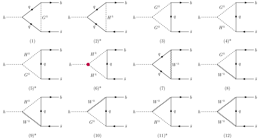
Figure 1: One-loop diagrams that contribute to the process $h\to b\bar{s}$. The quark $q$ inside the loops can be any $u$-type quark. The diagrams with an asterisk (*) do not appear in the SM. The red dot marks the $\lambda_{hH^{+}H^{-}}$ triple Higgs coupling.

All one-loop diagrams contributing to the process $h\to b\bar{s}$ in the 2HDM are depicted in Fig. 1. It should be noted that this process is loop induced because the $Z_{2}$ symmetry imposed in the 2HDM forbids flavor changing neutral currents at tree-level in the scalar sector. The total amplitude of the process can be written as:

$$\mathcal{M}\left(h\to b\bar{s}\right)=\frac{g^{3}}{64\pi^{2}m_{W}^{3}}\sum_{q=u,c,t}V_{qb}^{\ast}V_{qs}\bar{b}(p_{1})\left(\sum_{i=1}^{18}\mathcal{A}_{i}\right)s(p_{2}),$$ (11)

where $V_{ij}$ are the CKM matrix elements and $\mathcal{A}_{i}$ (with $i=1...18$) denotes the contribution to the amplitude of each of the 18 diagrams with the same numbering as shown in Fig. 1. $p_{1}$ and $p_{2}$ denote the momenta of the $b$ and $\bar{s}$ quarks, respectively. The explicit expressions of the 2HDM Feynman rules involved in the computation and the amplitudes $\mathcal{A}_{i}$ in the 2HDM can be found in Appendix A.

It should be noted that the particular fermions that are involved in this process are the various quarks, but not leptons, running in the loops and therefore, the prediction of the amplitude in the 2HDM types I and IV will be identical. Likewise, the prediction in types II and III will be also identical (see Tab. 2). The quark $q$ running inside the loops in Fig. 1 can be any $u$-type quark, accounting for a total of $18\times 3=54$ diagrams. All these diagrams are included in the computation of this decay. However, numerically some diagrams are more important than others. First, all contributions to the amplitude are proportional to either $m_{s}P_{R}$ or $m_{b}P_{L}$, where $P_{R,L}=(1\pm\gamma^{5})/2$ are the right/left chiral projectors. Since $m_{s}\ll m_{b}$, the contribution proportional to $P_{L}$ will dominate. On the other hand, concerning the $u$-type quark running inside the loop, the contribution from the $t$ quark is the leading one because it has the larger Yukawa couplings to Higgs bosons and the CKM suppression is milder with respect to other diagrams since $V_{tb}\simeq 1$. As said above, the computation reported here is a complete one with the inclusion of all the 54 diagrams present in the 2HDM. However, for illustrative purposes, approximate and simpler expressions considering only the leading contributions to ${\cal A}_{i}$ described above can be also found in Appendix A.

Finally, another important contribution in the 2HDM to the $h\to bs$ decay is the one coming from diagram 6, that depends on the triple Higgs coupling $\lambda_{hH^{+}H^{-}}$. In our convention, this triple Higgs coupling is dimensionless, such that the Feynman rule of the vertex $hH^{+}H^{-}$ is given by $-iv\lambda_{hH^{+}H^{-}}$. This coupling is a derived parameter within our setup of the 2HDM and its expression as a function of the input parameters $m_{h}$, $m_{H^{\pm}}$, $m_{12}$, $\tan\beta$ and $c_{\beta-\alpha}$ can be found in Eq. (10). It should be noticed that the coupling $\lambda_{hH^{+}H^{-}}$ does not vanish in the alignment limit, i.e. setting $c_{\beta-\alpha}=0$, and therefore neither does diagram 6. We will see later that this diagram and its interference effects with the rest of the diagrams is of crucial importance to the prediction of the decay width of $h\to bs$.

One key fact of the process $h\to bs$ is that it is very suppressed due to the unitarity of the CKM matrix. In particular, the unitarity relation that suppresses this decay is:

$$\sum_{q=u,c,t}V_{qb}^{\ast}V_{qs}=0\,.$$ (12)

Therefore, any contribution in the amplitudes ${\cal A}_{i}$ that does not depend on the mass of the $u$-type quark inside the loop, will factor out from the amplitude and vanish because of the unitarity of the CKM matrix. In order to find these $m_{q}$-independent parts of the amplitude, is crucial to perform the Passarino-Veltman reduction to scalar one-loop integrals in the amplitude. Thus, these terms in the amplitude were removed explicitly from the numerical evaluation.

Since this is a loop induced process, the full one-loop result should be free of ultraviolet divergences. The only non-divergent diagrams are diagrams 3 to 7, both included, and diagram 12, whereas the remaining diagrams are UV divergent. The total divergence in the amplitude sums up to:

$$\begin{split}\mathrm{div}(\mathcal{M})=\frac{g^{3}}{64\pi^{2}m_{W}^{3}}\sum_{q=u,c,t}V_{qb}^{\ast}V_{qs}\bar{b}\left(p_{1}\right)\left(m_{b}P_{L}+m_{s}P_{R}\right)s\left(p_{2}\right)\\ \times\Delta_{\mathrm{UV}}\left[m_{W}^{2}s_{\beta-\alpha}-\left(m_{q}^{2}\left(\xi_{d}-\xi_{u}\right)\left(\xi_{d}\xi_{u}+1\right)-\xi_{d}m_{W}^{2}\right)c_{\beta-\alpha}\right],\end{split}$$ (13)

where $\Delta_{\mathrm{UV}}=1/\epsilon=2/(4-D)$, $D=4-2\epsilon$ is the number of dimensions, and $\epsilon$ is a small parameter close to zero. If $c_{\beta-\alpha}=0$, one recovers the same divergence as in the SM, which vanishes thanks to the unitarity of the CKM matrix, in particular due to Eq. (12). Similarly, in the generic case with $c_{\beta-\alpha}\neq 0$ the terms proportional to $m_{W}^{2}$ also vanish because of the unitarity properties of the CKM matrix. The remaining terms proportional to $m_{q}^{2}$ vanish because the relation $\left(\xi_{d}-\xi_{u}\right)\left(\xi_{d}\xi_{u}+1\right)=0$ always holds in a $Z_{2}$ conserving 2HDM, see for instance Tab. 2.

The partial width of the process $h\to bs$ can be finally obtained as:

$$\Gamma(h\to bs)\equiv\Gamma(h\to b\bar{s})+\Gamma(h\to\bar{b}s)\simeq 2\times\Gamma(h\to b\bar{s})=2N_{C}\frac{\lambda^{1/2}\left(m_{h}^{2},m_{b}^{2},m_{s}^{2}\right)}{16\pi m_{h}^{3}}\left|\mathcal{\bar{M}}\right|^{2},$$ (14)

where $N_{C}=3$ is a color factor, $\lambda\left(x,y,z\right)=\left(x-y-z\right)^{2}-4y^{2}z^{2}$ and $\left|\mathcal{\bar{M}}\right|^{2}=\sum_{\mathrm{spin}}\left|\mathcal{M}\right|^{2}$ is the spin-averaged squared amplitude of Eq. (11). It should be noted that we have neglected the possible ${{\cal CP}}$ violating effects in this process, as we discussed at the beginning of this section.

3.1 $\Gamma\left(h\to bs\right)$ in the alignment limit

In this subsection, for illustrative purposes and to simplify the analysis, we will first restrict our study to the alignment limit, i.e. $c_{\beta-\alpha}=0$. Under this condition, the tree-level interactions of $h$ with fermions, gauge bosons and Goldstone bosons recover their SM value. Therefore, diagrams containing SM particles and the SM-like Higgs boson $h$ (i.e. diagrams without asterisk in Fig. 1) are as in the SM. In consequence, in the alignment limit, the new contributions to $h\to bs$ within the 2HDM arise only from diagrams with $H^{\pm}$ propagating in the loops. Hence, we can write the amplitude of $h\to bs$ as:

$$\mathcal{M}_{\rm align}\left(h\to b\bar{s}\right)=\frac{g^{3}}{64\pi^{2}m_{W}^{3}}\sum_{q=u,c,t}V_{qb}^{\ast}V_{qs}\bar{b}(p_{1})\bigg{[}{\cal A}_{\rm SM}+{\cal A}_{H^{\pm}}\bigg{]}s(p_{2}),$$ (15)

where ${\cal A}_{\rm SM}$ is the contribution from the SM-like diagrams in the alignment limit and ${\cal A}_{H^{\pm}}$ is the contribution from diagrams 2, 6, 14 and 17, those that feature a $H^{\pm}$ propagator in the loop. The remaining diagrams 4, 5, 9 and 11 vanish in the alignment limit.

In addition, for comparison, we have also computed the SM decay width under the same considerations described in the previous section and we have obtained the following value:

$$\Gamma_{\rm SM}\left(h\to bs\right)=4.22\times 10^{-10}\,\,\mathrm{GeV},$$ (16)

which is in agreement with the predictions in Refs. [5, 6]. We will use this value throughout this work to compare consistently the 2HDM prediction with the SM.

One interesting question here is, for which combination of 2HDM input parameters the SM prediction is recovered, corresponding to ${\cal A}_{H^{\pm}}=0$, see Eq. (15). One could expect naively that this ${\cal A}_{H^{\pm}}$ contribution should vanish for a very heavy $H^{\pm}$, since it appears suppressed by a factor $m_{H^{\pm}}^{-2}$ from each $H^{\pm}$ propagator. In fact, that is the case for the contributions from diagrams 2, 14 and 17. However, diagram 6 could exhibit some non-decoupling effects given the fact that $\lambda_{hH^{+}H^{-}}$ contains a term proportional to $m_{H^{\pm}}^{2}$. This coupling is non-zero in the alignment limit and has the following expression (see Eq. (10)):

$$\lambda_{hH^{+}H^{-}}^{\mathrm{align}}=\frac{m_{h}^{2}+2m_{H^{\pm}}^{2}-2\bar{m}^{2}}{v^{2}}.$$ (17)

For a very large value of $m_{H^{\pm}}$ the triangle loop function in diagram 6 scales $\propto m_{H^{\pm}}^{-2}$ (see Eqs. (45), (78), (79) and (80)), whereas the term in $\lambda_{hH^{+}H^{-}}\propto m_{H^{\pm}}^{2}$ gives rise to a non-vanishing contribution, which is constant with $m_{H^{\pm}}$ in this heavy mass limit. To suppress this contribution, one should then tune the prediction of $\lambda_{hH^{+}H^{-}}$ via a choice for $m_{12}$ such that $\lambda_{hH^{+}H^{-}}$ does not contain a term that depends quadratically on $m_{H^{\pm}}$. Nonetheless, it should be noted that outside the alignment limit one can still find BSM effects even with a heavy $H^{\pm}$ since the interaction $hH^{+}G^{-}$ is also proportional to $m_{H^{\pm}}^{2}$. This coupling can only be zero if $c_{\beta-\alpha}=0$ and/or if $m_{H^{\pm}}=m_{h}\simeq 125\,\,\mathrm{GeV}$.

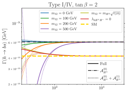
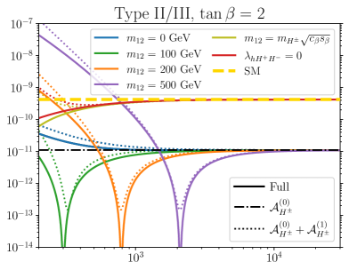
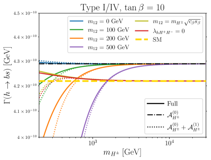
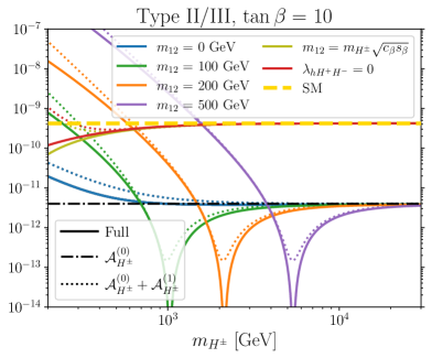
Figure 2: Prediction of $\Gamma(h\to bs)$ in the 2HDM types I and IV (left) and types II and III (right) as a function of $m_{H^{\pm}}$ in the alignment limit for $\tan\beta=2$ (top) and $\tan\beta=10$ (bottom) and for different values of $m_{12}$. Dot-dashed and dotted lines correspond to the 2HDM prediction of $\Gamma(h\to bs)$ with the charged Higgs boson effects approximated by a large $m_{H^{\pm}}$ expansion given by an effective vertex $V^{\rm eff}_{H^{\pm}}$, Eq. (23) with ${\cal A}_{H^{\pm}}^{\left(0\right)}$ (for the choices of fixed $m_{12}$) and ${\cal A}_{H^{\pm}}^{\left(0\right)}+{\cal A}_{H^{\pm}}^{\left(1\right)}$ respectively. Dashed yellow horizontal lines indicate the SM prediction.

The numerical prediction of $\Gamma(h\to bs)$ as a function of $m_{H^{\pm}}$, in the alignment limit, is shown in Fig. 2 for $\tan\beta=2$ (top) and $\tan\beta=10$ (bottom) for 2HDM types I/IV (left) and types II/III (right). The different solid color lines indicate several choices of the $m_{12}$ parameter. The SM prediction from Eq. (16) corresponds to the yellow dashed horizontal line. In this figure, one can see that the lines corresponding to $m_{12}=0,\,100,\,200,\,500\,\,\mathrm{GeV}$ tend at large $m_{H^{\pm}}$ to a fixed value of $\Gamma(h\to bs)\neq\Gamma_{\mathrm{SM}}(h\to bs)$. As we discussed above, this is because the non-decoupling contribution from diagram 6 due to the presence of $\lambda_{hH^{+}H^{-}}$. That constant value of $\Gamma\left(h\to bs\right)$ reached for large values of $m_{H^{\pm}}$ is larger than the SM value in types I/IV and smaller in types II/III. This implies that there is a constructive (destructive) interference between diagram 6 and the rest of the diagrams in types I/IV (II/III) for very large values of $m_{H^{\pm}}$. Hence, those negative interference effects lead to the deep dips found in the prediction of the partial width in types II/III. Conversely, regions with $\bar{m}\;\raisebox{-3.00003pt}{$\stackrel{{\scriptstyle\displaystyle>}}{{\sim}}$}\;m_{H^{\pm}}$ which imply $\lambda_{hH^{+}H^{-}}\;\raisebox{-3.00003pt}{$\stackrel{{\scriptstyle\displaystyle<}}{{\sim}}$}\;0$ show smaller $\Gamma\left(h\to bs\right)$ in the 2HDM than in the SM in types I/IV, while in types II/III the 2HDM rates are larger than in the SM, probing these interference patterns. These different patterns among the various types can traced back to the different signs of $\xi_{d}$ between 2HDM types I/IV and II/III, that enter in the Yukawa interactions of $H^{\pm}$ (see Eq. (6) and Tab. 2).

On the other hand, the red solid line in each plot of Fig. 2 corresponds to a value of $m_{12}$ such that the coupling $\lambda_{hH^{+}H^{-}}$ in Eq. (17) is equal to zero. Therefore in that case the only remnant 2HDM contribution in $\mathcal{A}_{H^{\pm}}$ comes from diagrams 2, 14 and 17. For all 2HDM types, this line reach the SM prediction for $m_{H^{\pm}}\gtrsim 2\,\,\mathrm{TeV}$, just as expected. The olive line indicates the prediction for the choice $m_{12}=m_{H^{\pm}}\sqrt{\cos\beta\sin\beta}$ (or equivalently $\bar{m}=m_{H^{\pm}}$), which implies the particular setting of $\lambda_{hH^{+}H^{-}}=m_{h}^{2}/v^{2}$. In this case, since $\lambda_{hH^{+}H^{-}}$ does not depend on $m_{H^{\pm}}$, there is not a non-decoupling effect from diagram 6 and the prediction for $\Gamma\left(h\to bs\right)$ also reaches the SM value for sufficiently large $m_{H^{\pm}}$.

In fact, the appearing gap at large $m_{H^{\pm}}$ between the predictions with a fixed value of $m_{12}$ and the red line with $\lambda_{hH^{+}H^{-}}=0$, or the olive line with $\lambda_{hH^{+}H^{-}}=m_{h}^{2}/v^{2}$ highlights the non-decoupling contribution from diagram 6 for parameter choices that lead to $\lambda_{hH^{+}H^{-}}\propto m_{H^{\pm}}^{2}$. It also confirms that the interference effects discussed above are caused by the presence of diagram 6, and consequently, the value of $\lambda_{hH^{+}H^{-}}$ is crucial in the 2HDM prediction of $\Gamma\left(h\to bs\right)$.

3.2 One-loop effective $hbs$ vertex from the large $m_{H^{\pm}}$ expansion

Given the presence of possible decoupling and non-decoupling effects in $\Gamma\left(h\to bs\right)$ described in the previous section, here we present a large $m_{H^{\pm}}$ series expansion that will capture such effects. We work again in the alignment limit, i.e, we set $c_{\beta-\alpha}=0$. The analytical results will be presented in the form of a one-loop effective vertex, $V^{\rm eff}_{H^{\pm}}$, for the $hbs$ interaction generated from integrating out the heavy mode $H^{\pm}$, which is valid at large $m_{H^{\pm}}$. Such an effective vertex can be useful to obtain a rough estimate of the most relevant numerical contributions from $H^{\pm}$ to the $h\to bs$ decay rates in the 2HDM.

In order to obtain this effective vertex, we have performed a series expansion of the 2HDM contribution $\mathcal{A}_{H^{\pm}}^{\rm eff}$ in powers of a small dimensionless variable $x_{H^{\pm}}$, assuming that

$$x_{H^{\pm}}=m_{\rm EW}^{2}/m_{H^{\pm}}^{2}\ll 1,$$ (18)

where $m_{\rm EW}$ denotes generically any mass-dimension parameter (other than $m_{H^{\pm}}$) involved in the computation, i.e. $m_{h}$, $m_{W}$, $m_{q}$ and $m_{12}$. Furthermore, for the results in this section, we have considered only the dominant contributions to ${\cal A}_{H^{\pm}}$, which are globally proportional to $m_{t}^{2}m_{b}$. In summary, the validity of our assumptions in this section applies in practice to the following mass hierarchy: $m_{H^{\pm}}\gg m_{t},\ m_{h},\ m_{12}\gg m_{b}\gg m_{s},\ m_{c},\ m_{u}$. (The case $m_{H^{\pm}}\sim m_{12}$ will be discussed separately below.) This hierarchy, on the other hand, (as discussed in the beginning of Sect. 3) implies that the result for the effective vertex will only involve the left projector $P_{L}$, since the $P_{R}$ contribution is always proportional to $m_{s}$ and can therefore be safely neglected. The analytical computation presented below was performed with the help of the public code PackageX [23].

We have computed the first two contributions in this series expansion,

$$\mathcal{A}_{H^{\pm}}^{\rm eff}=\mathcal{A}_{H^{\pm}}^{\left(0\right)}+\mathcal{A}_{H^{\pm}}^{\left(1\right)}+\dots$$ (19)

where $\mathcal{A}_{H^{\pm}}^{\left(0\right)}$ is the leading order contribution, i.e. $\mathcal{O}(x_{H^{\pm}}^{0})$, and $\mathcal{A}_{H^{\pm}}^{\left(1\right)}$ is the next to leading order contribution, i.e. $\mathcal{O}(x_{H^{\pm}}^{1})$. The dots in the above equation correspond to terms of $\mathcal{O}(x_{H^{\pm}}^{n})$, with $n=2,3,..$. In the following of this subsection we first present the analytical results of $\mathcal{A}_{H^{\pm}}^{\left(0\right)}$ and $\mathcal{A}_{H^{\pm}}^{\left(1\right)}$ in the generic case where $\lambda_{hH^{+}H^{-}}$ has been replaced by the expression in the alignment limit given by Eq. (17). Subsequently, we compare them with the analytical results of the two cases with the particular choices of $\lambda_{hH^{+}H^{-}}=0$ and $\lambda_{hH^{+}H^{-}}=m_{h}^{2}/v^{2}$.

The result obtained for the leading order contribution is the following:

$$\mathcal{A}_{H^{\pm}}^{\left(0\right)}=m_{t}^{2}m_{b}P_{L}\xi_{u}\biggl{\{}\frac{1}{2}\xi_{u}-2\xi_{d}\biggr{\}}\,.$$ (20)

This is the non-decoupling contribution (valid under the above given assumptions) discussed in the previous section that comes solely from diagram 6. With the particular values of $\xi_{u}$ and $\xi_{d}$ from Tab. 2 in Eq. (20), we get the following non-decoupling effects for the four 2HDM types:

$$\mathcal{A}_{H^{\pm}}^{\left(0\right)}=\begin{cases}-\frac{3}{2}m_{t}^{2}m_{b}P_{L}\cot^{2}\beta&\mathrm{Types\ I/IV},\vspace{2mm}\\ \frac{1}{2}m_{t}^{2}m_{b}P_{L}\left(4+\cot^{2}\beta\right)&\mathrm{Types\ II/III}.\end{cases}$$ (21)

Hence, $\mathcal{A}_{H^{\pm}}^{\left(0\right)}$ has different signs in types I/IV and II/III in the large $m_{H^{\pm}}$ limit.

The result for the next to leading order contribution is the following:

$$\begin{split}&\mathcal{A}_{H^{\pm}}^{\left(1\right)}=\frac{m_{t}^{2}m_{b}P_{L}\xi_{u}}{36m_{H^{\pm}}^{2}}\left\{36\bar{m}^{2}\left(2\xi_{d}-\frac{1}{2}\xi_{u}\right)+m_{h}^{2}(11\xi_{u}-46\xi_{d})-120m_{t}^{2}\xi_{d}\right.\\ &\left.+12\xi_{d}\left(2\left(m_{h}^{2}+5m_{t}^{2}\right)\sqrt{4r-1}\ \mathrm{arccot}\left(\sqrt{4r-1}\right)-m_{h}^{2}\log\left(\frac{m_{H^{\pm}}^{2}}{m_{t}^{2}}\right)\right)\right\}\,,\end{split}$$ (22)

with $r=m_{t}^{2}/m_{h}^{2}$. In the above result, the effects from $H^{\pm}$ are suppressed by $m_{H^{\pm}}^{-2}$ and come from diagrams 2, 6 and 14. Diagram 17 is proportional to $m_{s}$ and therefore negligible in our approximations. A more detailed derivation of the above equations can be found in Appendix B.

In summary, and for practical purposes, the effects from the $H^{\pm}$ in the alignment limit to the $h\to bs$ decay rates can be approximated by a one-loop effective $hbs$ vertex $V^{\rm eff}_{H^{\pm}}$, whose value, according to Eq. (11), is given by:

$$\begin{gathered}\includegraphics[scale={.9}]{hbs-effective}\end{gathered}:\ \ \ \ V^{\rm eff}_{H^{\pm}}\ =\ \frac{g^{3}}{64\pi^{2}m_{W}^{3}}V_{tb}^{\ast}V_{ts}\;{\cal A}_{H^{\pm}}^{\rm eff}\;,$$ (23)

where ${\cal A}_{H^{\pm}}^{\rm eff}$, as defined in Eq. (19), receives contributions from leading order and next to leading order in $x_{H^{\pm}}$ as given in Eqs. (20)-(22).

The approximate prediction for $\Gamma\left(h\to bs\right)$ with the effects of the heavy $H^{\pm}$ described by the effective vertex in Eq. (23) is also shown in Fig. 2 for the cases of fixed $m_{12}$ values. Both results with $V^{\rm eff}_{H^{\pm}}$ given by the leading order contribution, ${\cal A}_{H^{\pm}}^{\left(0\right)}$ (dot-dashed lines), and by the sum of the leading and next to leading contributions, ${\cal A}_{H^{\pm}}^{\left(0\right)}+{\cal A}_{H^{\pm}}^{\left(1\right)}$ (dotted lines) are shown for the different fixed values of $m_{12}$.

One can see that the approximation given by ${\cal A}_{H^{\pm}}^{\left(0\right)}$ already works quite well, specially for large values of $m_{H^{\pm}}$, just as expected. For example, for $m_{12}=0$, this approximation is very close to the full prediction in type I/IV for values of $m_{H^{\pm}}$ around hundreds of GeV while for types II/III the approximation works fine from around 1 TeV. As expected, for the lines with larger values of $m_{12}$, it is required to go to larger values of $m_{H^{\pm}}$ in order that ${\cal A}_{H^{\pm}}^{\left(0\right)}$ be a good approximation of ${\cal A}_{H^{\pm}}$. Also, this leading order approximation can reproduce quite well the dependence of the non-decoupling contributions for different values of $\tan\beta$. In fact, this leading contribution can already describe that the gap between the SM and the 2HDM non-decoupling value increases with $\tan\beta$ in types II/III and decreases in types I/IV.

Turning to the prediction with the effective vertex including both leading and next to leading order contributions, ${\cal A}_{H^{\pm}}^{\left(0\right)}+{\cal A}_{H^{\pm}}^{\left(1\right)}$, we also see in Fig. 2 that it approximates better the full result than considering just the leading order, in particular in the low $m_{H^{\pm}}$ region where the ${\cal O}(m_{\rm EW}^{2}/m_{H^{\pm}}^{2})$ corrections are more relevant. Furthermore, in types II/III, it also reproduces with a good accuracy the location of the deep interference minima present in these types, particularly if it takes place for a large value of $m_{H^{\pm}}$.

Finally, we comment on the effective vertex approximation for choices of $m_{12}$ that do not lead to the dependence of $\lambda_{hH^{+}H^{-}}\propto m_{H^{\pm}}^{2}$ for large values of $m_{H^{\pm}}$. In Fig. 2 this is realized for the particular choice of $m_{12}^{2}=m_{H^{\pm}}^{2}\sin\beta\cos\beta$ that leads to $\lambda_{hH^{+}H^{-}}=m_{h}^{2}/v^{2}$, and for the choice of $m_{12}^{2}=\sin\beta\cos\beta\left(m_{H^{\pm}}^{2}+m_{h}^{2}/2\right)$ that leads to $\lambda_{hH^{+}H^{-}}=0$. For these parameter choices, $m_{12}^{2}$ is constrained to contain a term directly proportional to $m_{H^{\pm}}^{2}$, i.e., the required expansion condition $m_{12}\ll m_{H^{\pm}}$ shown in Eq. (19) is not satisfied. Therefore, the consistent way to perform the series expansion in these cases is to consider the particular expression for $m_{12}$, and the resulting value of $\lambda_{hH^{+}H^{-}}$, before the series expansion. As noted above, the absence of a term proportional to $m_{H^{\pm}}^{2}$ in $\lambda_{hH^{+}H^{-}}$ implies complete decoupling in the prediction of $\Gamma(h\to bs)$ for large values of $m_{H^{\pm}}$. Thus, for both scenarios, after doing the expansion, we find a vanishing leading term:

$${\cal A}_{H^{\pm}}^{\left(0\right)}=0\,,$$ (24)

which summarizes the absence of non-decoupling effects in these two cases. However, there are still non-vanishing contributions to ${\cal A}_{H^{\pm}}^{\left(1\right)}$, which are suppressed by $m_{H^{\pm}}^{2}$ and therefore summarize the decoupling effects in these two particular cases. If $\lambda_{hH^{+}H^{-}}=0$, the result for the next to leading order contribution is:

$$\begin{split}&\mathcal{A}_{H^{\pm}}^{\left(1\right)}=\frac{m_{t}^{2}m_{b}P_{L}\xi_{u}}{36m_{H^{\pm}}^{2}}\bigg{\{}-4m_{h}^{2}\xi_{d}+6m_{t}^{2}\left(3\xi_{u}-8\xi_{d}\right)\\ &\left.+12\xi_{d}\left(2\left(m_{h}^{2}+5m_{t}^{2}\right)\sqrt{4r-1}\ \mathrm{arccot}\left(\sqrt{4r-1}\right)-\left(m_{h}^{2}+6m_{t}^{2}\right)\log\left(\frac{m_{H^{\pm}}^{2}}{m_{t}^{2}}\right)\right)\right\}\,,\end{split}$$ (25)

which only receives contributions from diagrams 2 and 14. On the other hand, if $m_{12}=m_{H^{\pm}}\sqrt{\sin\beta\cos\beta}$, corresponding to $\lambda_{hH^{+}H^{-}}=m_{h}^{2}/v^{2}$, the result for ${\cal A}_{H^{\pm}}^{\left(1\right)}$ also receives contributions from diagram 6. In this case the result is:

$$\begin{split}&\mathcal{A}_{H^{\pm}}^{\left(1\right)}=\frac{m_{t}^{2}m_{b}P_{L}\xi_{u}}{36m_{H^{\pm}}^{2}}\bigg{\{}m_{h}^{2}\left(9\xi_{u}-40\xi_{d}\right)+6m_{t}^{2}\left(3\xi_{u}-8\xi_{d}\right)\\ &\left.+12\xi_{d}\left(2\left(m_{h}^{2}+5m_{t}^{2}\right)\sqrt{4r-1}\ \mathrm{arccot}\left(\sqrt{4r-1}\right)-\left(m_{h}^{2}+6m_{t}^{2}\right)\log\left(\frac{m_{H^{\pm}}^{2}}{m_{t}^{2}}\right)\right)\right\}\,.\end{split}$$ (26)

It should be noted that the two expressions above are different from the previous result of Eq. (22), as expected. In that result, there are additional decoupling contributions of $\mathcal{O}\left(m_{H^{\pm}}^{-2}\right)$ coming from diagram 6 that are absent if $m_{12}=m_{H^{\pm}}\sqrt{\sin\beta\cos\beta}$ or $\lambda_{hH^{+}H^{-}}=0$.

The numerical results of the effective vertex considering the explicit expressions of $\mathcal{A}_{H^{\pm}}^{\left(1\right)}$ in the effective vertex $V_{H^{\pm}}^{\mathrm{eff}}$ are also shown in Fig. 2. The dotted red line shows the result from the approximation in the case that $\lambda_{hH^{+}H^{-}}=0$ (Eq. (25)), while the dotted olive line shows the result of the approximation for $\bar{m}=m_{H^{\pm}}$ (Eq. (26)). Since $\mathcal{A}_{H^{\pm}}^{\left(0\right)}=0$ in both cases, they can reproduce the expected decoupling behavior given these parameter choices for $m_{12}$. Additionally, the convergence to the SM prediction is also well reproduced by the effective vertex approximation considering the results for $\mathcal{A}_{H^{\pm}}^{\left(1\right)}$ for both cases. In particular, the approximation yields a very good agreement with the complete prediction when $m_{H^{\pm}}\gtrsim 500\,\,\mathrm{GeV}$.

3.3 $\Gamma\left(h\to bs\right)$ outside the alignment limit

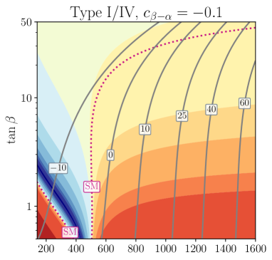
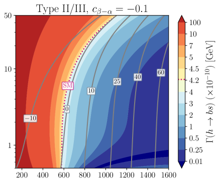
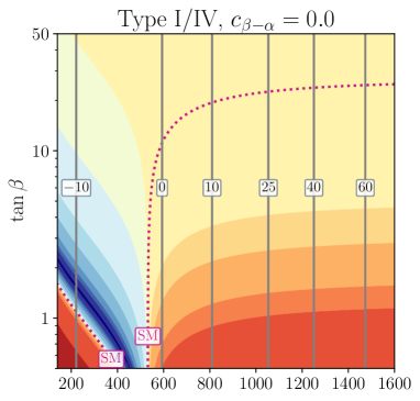
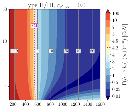
Figure 3: Prediction of $\Gamma(h\to bs)$ in the plane $m_{H^{\pm}}$-$\tan\beta$ with $\bar{m}=600\,\,\mathrm{GeV}$ for 2HDM types I/IV (left column) and types II/III (right column). $c_{\beta-\alpha}$ is set to -0.1 (top), 0 (middle) and 0.1 (bottom). Dotted pink line corresponds to the SM prediction. Solid grey lines show contour lines for different values of $\lambda_{hH^{+}H^{-}}$.

Once we studied the behavior of $\Gamma(h\to bs)$ within the alignment limit, the next step is to consider this observable outside this limit. The fact that $c_{\beta-\alpha}\neq 0$ implies that the couplings of $h$ to the fermions, gauge bosons and Goldstone bosons are not SM-like. Consequently, deviations with respect to the SM can arise from all diagrams. The $h$ coupling to fermions scales with $\xi_{f}^{h}=s_{\beta-\alpha}+\xi_{f}c_{\beta-\alpha}$ (see Eq. (6)). Regarding the $h$ couplings to gauge and Goldstone bosons, they are now proportional to $s_{\beta-\alpha}$ and Yukawa-type independent, and consequently they are always smaller than or equal to the SM Higgs-boson couplings. Furthermore, another interactions involving the charged Higgs boson $H^{\pm}$ are now also present in the prediction, like $hH^{\pm}G^{\mp},\ hH^{\pm}W^{\mp}\propto c_{\beta-\alpha}$, and consequently they will depend on the sign of $c_{\beta-\alpha}$ and will be potentially small if $c_{\beta-\alpha}$ is also small. Finally, the last new effect can enter thought $\lambda_{hH^{+}H^{-}}$, that is a function of $c_{\beta-\alpha}$ given in Eq. (10). Due to these features appearing outside the alignment limit, it is not possible to split the 2HDM result for the decay amplitude into the SM and the $H^{\pm}$ contributions as in Eq. (15), and neither to write the (possibly) most relevant contribution from the 2HDM by means of just an effective vertex for very large $m_{H^{\pm}}$ as in Eq. (23). Thus, we present in this section the numerical results using the full formulas for the decay amplitude and we do not employ anymore the approximate formulas with the effective vertex discussed in the previous section. Since we investigate here the analytical dependencies of $\Gamma(h\to bs)$ we do not apply any experimental or theoretical constraints. This will be done in the phenomenological analysis in Sect. 4.

In Fig. 3 we show the effects of $c_{\beta-\alpha}\neq 0$ on $\Gamma(h\to bs)$ in the plane $m_{H^{\pm}}$-$\tan\beta$ with $\bar{m}=600\,\,\mathrm{GeV}$ for the 2HDM types I/IV (left column) and II/III (right column). The prediction for $c_{\beta-\alpha}=-0.1,\;0.0,\;0.1$ is shown for both cases in the top, middle and bottom rows, respectively. The dotted pink contour lines indicates where the partial decay width has the same value as in the SM. The grey contour lines in the plots correspond to constant values of the triple Higgs coupling $\lambda_{hH^{+}H^{-}}$, i.e. the parameter that controls to a large extend the size of the contribution of diagram 6.

We first focus on the plots in the alignment limit as shown in the middle row of Fig. 3. In types I/IV (middle left plot), we see that for $\lambda_{hH^{+}H^{-}}\;\raisebox{-3.00003pt}{$\stackrel{{\scriptstyle\displaystyle<}}{{\sim}}$}\;0\,(\;\raisebox{-3.00003pt}{$\stackrel{{\scriptstyle\displaystyle>}}{{\sim}}$}\;0)$ very important destructive (constructive) interference effects are found. These interference effects are mainly dominated by the effect of diagram 6, the one containing $\lambda_{hH^{+}H^{-}}$, just as we found in the previous section. In fact, there is a narrow region where the prediction of the partial width can be below $10^{-12}\,\,\mathrm{GeV}$, just in the region where $\lambda_{hH^{+}H^{-}}$ becomes negative. If we turn now to the prediction in types II and III (middle right plot), the situation is the opposite as compared to types I and IV. Now the strong destructive effects are found when $\lambda_{hH^{+}H^{-}}\;\raisebox{-3.00003pt}{$\stackrel{{\scriptstyle\displaystyle>}}{{\sim}}$}\;0$, while in the region where $\lambda_{hH^{+}H^{-}}\;\raisebox{-3.00003pt}{$\stackrel{{\scriptstyle\displaystyle<}}{{\sim}}$}\;0$ they are absent. It can also be seen that the contour lines become flat for larger values of $m_{H^{\pm}}$, these are the non-decoupling effects for fixed $m_{12}$ that, as discussed in the previous section, can be approximated by Eq. (20). In the case of types II/III it would be necessary to go to larger values of $m_{H^{\pm}}$ to reach this flat behavior. Furthermore, we can also see the effects of large $\tan\beta$ in these plots. In types I/IV, it can be observed that the prediction of $\Gamma(h\to bs)$ exhibits a strong dependence on $\tan\beta$ for lower values of this parameter, whereas the dependence is less pronounced in the region of large $\tan\beta$. This is because all diagrams with a $H^{\pm}$ running inside the loop are proportional to $\xi_{d}=\cot\beta$, so they are very suppressed in this region of large $\tan\beta$. Nonetheless, in types II/III, $\xi_{d}=-\tan\beta$ and these diagrams are relevant when $\tan\beta$ is large. In fact, some leading contributions are proportional to $\xi_{u}\xi_{d}$, and therefore in these 2HDM types we see $\tan\beta$ independence in the contour lines for $\Gamma\left(h\to bs\right)$.

We turn now to the cases where $c_{\beta-\alpha}\neq 0$. We can understand these results as distortions from the alignment limit case. In types I/IV, we see that overall the partial width is slightly larger (smaller) when $c_{\beta-\alpha}=-0.1(+0.1)$ with respect to the alignment limit case, specially for large values of $m_{H^{\pm}}$. The reason for this behavior is that the SM-like diagrams are slightly enhanced for $c_{\beta-\alpha}>0$ and diminished for $c_{\beta-\alpha}>0$, and thus account for these subtle differences. Now we turn to types II/III, where we see noticeable differences between the plots with $c_{\beta-\alpha}=\pm 0.1$ and the prediction in the alignment limit, contrary to what we have seen in types I/IV. As before, the contribution from diagram 6 dominates the pattern of the prediction of $\Gamma\left(h\to bs\right)$ for low and moderate values of $\tan\beta\;\raisebox{-3.00003pt}{$\stackrel{{\scriptstyle\displaystyle<}}{{\sim}}$}\;5$, where the prediction is very similar to the alignment limit case. However, in the large $\tan\beta$ region there is a new non-negligible 2HDM effect coming from diagram 14, which can be enhanced by $\xi_{d}=-\tan\beta$. In addition, the SM-like diagrams can be also strongly enhanced by the same parameter, like for example diagram 13. Furthermore, because of the interplay between all these contributions, the deep minimum due to the negative interference can be found around $\tan\beta\simeq 20$ for lower values of $m_{H^{\pm}}$ and $c_{\beta-\alpha}=+0.1$.

It should be noted that the SM prediction, corresponding to the pink dashed contours in Fig. 3 is found in both sets of Yukawa types (I and IV vs. II and III) in different regions of the parameter space. In contrast to our discussion of the alignment limit in Sect. 3.1, in these regions the sum of the SM-like diagrams do not yield the SM value: their non-SM contributions are canceled by the non-SM diagrams involving the $H^{\pm}$.

4 Allowed values of $\mathrm{BR}\left(h\to bs\right)$ in the 2HDM

After the theoretical study of the prediction of $\Gamma\left(h\to bs\right)$, in this section we will analyze the possible size for the branching ratio still allowed by the current theoretical and experimental constraints of the 2HDM. The restrictions on the parameter space for the 2HDM was studied recently in Ref. [18, 17]. Here we follow the same procedure and only briefly summarize the considered constraints:

• Electroweak precision data. New physics effects on electroweak observables from extended Higgs sectors can be parametrized in terms of the oblique parameters $S$, $T$ and $U$ [24, 25]. The values for the oblique parameters reported by the PDG [26] are very close to zero, meaning that the new physics contribution should remain small. Within the 2HDM, the most constraining oblique parameter is $T$, that is very sensitive to mass splittings between the additional Higgs bosons. Therefore, in the rest of this work, we will consider $m_{A}=m_{H^{\pm}}$, because this choice keeps the $T$ under control at the one-loop level, even outside the alignment limit.

• Theoretical constraints. These constraints consists in tree-level perturbative unitarity and the stability of the 2HDM potential. For the tree-level unitarity, we set an upper bound on the modulus of the eigenvalues of the two-body $s$-wave scattering amplitude matrix between the scalars fields [28, 29, 30]. For potential stability, we demand the 2HDM potential to be bounded from below [31, 32]. Additionally, we also require that the minimum of the potential is a true minimum [33]. All these constraints can be translated to inequalities involving the parameters $\lambda_{i}$ from the 2HDM potential in Eq. (1) and can be found in Ref. [18]. Typically, these theoretical constraints impose the hardest bounds on the tripe Higgs couplings size and, in particular, on $\lambda_{hH^{+}H^{-}}$.

• Higgs searches at colliders. We require that the Higgs bosons predicted by the 2HDM avoid the known experimental searches for new particles at the 95% CL. We made use of the public code HiggsBounds5.9 [34, 35, 36, 37, 38, 39], that determines if a particular configuration of an extended-Higgs model is excluded at the 95% CL by the existing experimental bounds. The theoretical predictions required by HiggsBounds to check the experimental bounds were computed with the public code 2HDMC [40]. HiggsBounds contains experimental bounds from LEP, Tevatron and the LHC, including also all relevant results from the LHC Run 2.

• Rate measurements of the 125 GeV Higgs boson. We have identified the $h$ state from the 2HDM with the $~{}125\,\,\mathrm{GeV}$ SM-like Higgs boson discovered by the LHC. The properties of $h$ should be in agreement with the experimental measurements of the mass and the signal strengths of such Higgs boson. To evaluate this agreement we made use of the public code HiggsSignals2.6 [41, 42, 43, 39], that performs a statistical $\chi^{2}$ analysis considering all the Higgs boson signal strength and mass measurements available from Tevatron and the LHC, including most relevant results from the LHC Run 2. Again, the theoretical predictions needed by HiggsSignals to compute the $\chi^{2}$ fit are obtained with 2HDMC. We will consider the allowed region to be not further away than $2\sigma$ ($\Delta\chi^{2}=6.18$ for a two-dimensional scan, i.e. a plane) from the SM, where $\chi^{2}_{\rm SM}=85.76$ with 107 observables. It is known that the discovered Higgs boson is in a very good agreement with the SM predictions, therefore the results from HiggsSignals will be translated into allowed values of $c_{\beta-\alpha}$ very close the alignment limit. Stronger constraints on $c_{\beta-\alpha}$ are expected in types II, III and IV, where the $h\to bb$ and/or the $h\to\tau\tau$ rates are enhanced by large values of $\tan\beta$ (depending on the type, see Tab. 2).

• Flavor observables. The new Higgs bosons in the 2HDM can induce relevant loop corrections to several rare $b$-flavored meson decays. In many BSM models the most important new contributions to these $B$-physics observables come from the effects from diagrams mediated by charged Higgs bosons, $H^{\pm}$. In our analysis, we will consider the 95% CL limits from the experimental average of $\text{BR}\left(B\to X_{s}\gamma\right)$ and $\text{BR}\left(B_{s}\to\mu\mu\right)$, as given in [26]. The theoretical computation of these BRs within the 2HDM was done with the public codes SuperISO [44, 45] and 2HDMC. Stronger bounds are known to be found for all types in the low $\tan\beta$ region with light $H^{\pm}$. Furthermore, in types II and III, there is a nearly $\tan\beta$-independent bound on $m_{H^{\pm}}\;\raisebox{-3.00003pt}{$\stackrel{{\scriptstyle\displaystyle>}}{{\sim}}$}\;500\,\,\mathrm{GeV}$.

4.1 Results of $\mathrm{BR}\left(h\to bs\right)$

The results in this section will be given in terms of the ratio between the $\text{BR}\left(h\to bs\right)$ prediction in the 2HDM with respect to the SM, given by:

$$R_{\mathrm{2HDM}}=\frac{\text{BR}\left(h\to bs\right)_{\mathrm{2HDM}}}{\text{BR}\left(h\to bs\right)_{\mathrm{SM}}}.$$ (27)

The computation of the total width of $h$ needed to estimate $\text{BR}\left(h\to bs\right)_{\rm 2HDM}$ was done with the public code 2HDMC [40]. For the $\text{BR}\left(h\to bs\right)_{\rm SM}$ prediction we used the following value of the total width:

$$\Gamma_{\mathrm{SM}}\left(h\right)=4.353\times 10^{-3}\,\,\mathrm{GeV},$$ (28)

obtained with 2HDMC via setting $c_{\beta-\alpha}=0$ and $\lambda_{hH^{+}H^{-}}=0$ via a tuned value of $m_{12}$. This choice allows for a consistent comparison of both quantities at the same accuracy level.

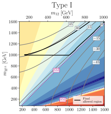
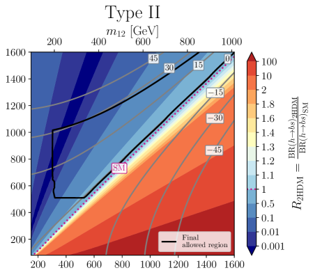
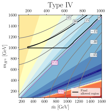
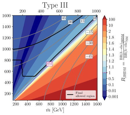
Figure 4: Prediction of $R_{\mathrm{2HDM}}=\text{BR}\left(h\to bs\right)_{\mathrm{2HDM}}/\text{BR}\left(h\to bs\right)_{\mathrm{SM}}$ in the plane $\bar{m}$-$m_{H^{\pm}}$ with $m_{h}=125\,\,\mathrm{GeV}$, $m_{H}=\bar{m}+50\,\,\mathrm{GeV}$, $m_{A}=m_{H^{\pm}}$, $\tan\beta=2$ and $c_{\beta-\alpha}=0$ for the four 2HDM types. The black contour lines indicates the boundary of the allowed region by all considered constraints. The dashed pink contour correspond to $R_{\mathrm{2HDM}}=1$. Solid grey lines shows contour lines with different values of $\lambda_{hH^{+}H^{-}}$.

In Fig. 4 we show the prediction for $R_{\mathrm{2HDM}}$ in the plane $m_{H^{\pm}}$-$\bar{m}$ in the alignment limit for $\tan\beta=2$, $m_{h}=125\,\,\mathrm{GeV}$, $m_{H}=\bar{m}-50\,\,\mathrm{GeV}$ and $m_{A}=m_{H^{\pm}}$. The $R_{\mathrm{2HDM}}$ prediction for types I/IV are shown in the left column of the figure, while the 2HDM types II/III predictions are shown in the right column. In the upper axis we show the corresponding value of $m_{12}$, which is related to $\bar{m}$ by the equation $m_{12}^{2}=\bar{m}^{2}\sin\beta\cos\beta=\frac{2}{5}\bar{m}^{2}$, for the chosen value of $\tan\beta$. Since we are in the alignment limit, our prediction for the total width of $h$ does not depend on the model type and therefore the values of $\text{BR}\left(h\to bs\right)$ are equal in types I/IV and in types II/III.

First, we comment on the shape of the allowed area by our set of constraints in the four types, whose boundaries are shown as solid black lines. For all types, there is a diagonal line, close to $m_{H^{\pm}}=\bar{m}$, coming from the potential stability constraints. On the other hand, the boundary close to the $\lambda_{hH^{+}H^{-}}=30$ contour corresponds to tree-level unitarity. These theoretical constraints are model independent and therefore equal for the four types. The lower bound for $m_{H^{\pm}}$ in all types comes from $B\to X_{s}\gamma$ for types I/IV and from $B_{s}\to\mu\mu$ for types II/III. Finally, there are some disallowed areas in types II/III for low values of $\bar{m}$ due to BSM Higgs-boson searches. In both types, the bound below $m_{H^{\pm}}\sim 800\,\,\mathrm{GeV}$ originates from a BSM search in the $pp\to H,\,A\to\tau\tau$ channel [47], while the additional bound in type III for $m_{H^{\pm}}\;\raisebox{-3.00003pt}{$\stackrel{{\scriptstyle\displaystyle>}}{{\sim}}$}\;800\,\,\mathrm{GeV}$ comes from a $gg\to A\to HZ\to bbll$ search [48].

Now, we turn to the discussion on the values for $R_{\mathrm{2HDM}}$ in Fig. 4. Overall, the contour lines for $R_{\mathrm{2HDM}}$ follow straight lines with different slopes in the $m_{H^{\pm}}$-$\bar{m}$ plane. This reflects the dependence of the diagram 6 amplitude on these parameters, which is the dominant contribution to the process, as we have discussed above. Furthermore, the same interference pattern as before can be observed: in types I/IV, for $\lambda_{hH^{+}H^{-}}\;\raisebox{-3.00003pt}{$\stackrel{{\scriptstyle\displaystyle>}}{{\sim}}$}\;0\left(\;\raisebox{-3.00003pt}{$\stackrel{{\scriptstyle\displaystyle<}}{{\sim}}$}\;0\right)$ the interference is constructive (destructive), and the opposite happens in types II/III. Since negative values for $\lambda_{hH^{+}H^{-}}$ are disallowed by the theoretical constraints [17, 18], inside the allowed region we find an enhancement w.r.t. the SM prediction in types I/IV ($R_{\mathrm{2HDM}}>1$) and a decrease w.r.t. the SM ($R_{\mathrm{2HDM}}<1$) in types II/III. In particular, in this plane for types I/IV, $R_{\mathrm{2HDM}}$ can reach values up to 1.4 close to the left “tip” of the allowed region, around $m_{H^{\pm}}\sim 1\,\,\mathrm{TeV}$ and $\bar{m}\sim 300\,\,\mathrm{GeV}$ (or $m_{12}\sim 200\,\,\mathrm{GeV}$). In types II/III, $R_{\mathrm{2HDM}}$ can be orders of magnitude smaller than 1, just around that same region. In principle, there should be a contour line where $R_{\mathrm{2HDM}}$ is exactly zero, but numerically that is not possible, and we find values as low as $R_{\mathrm{2HDM}}\sim 10^{-9}$, inside and outside the allowed region. As a consequence of this destructive interference pattern, it is very difficult to find values for $\text{BR}\left(h\to bs\right)$ larger than the SM prediction within the allowed region in types II/III.

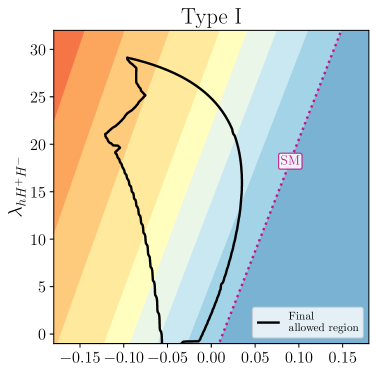
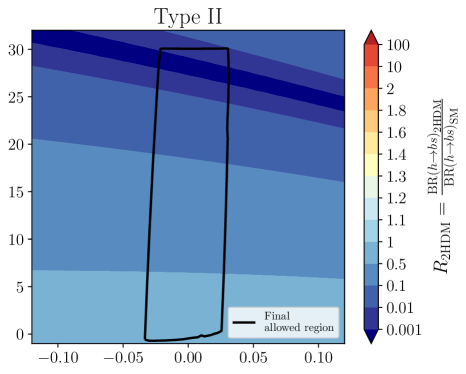
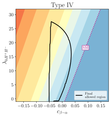
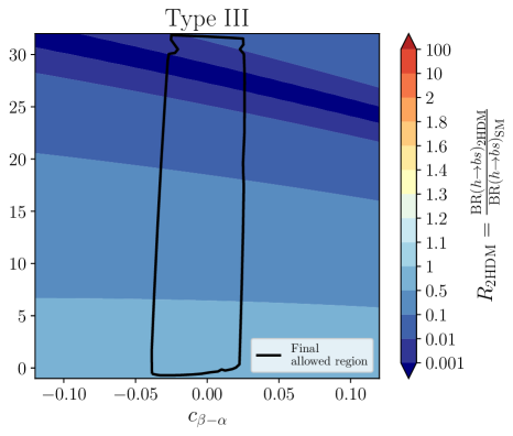
Figure 5: Prediction of $R_{\mathrm{2HDM}}$ in the plane $\lambda_{hH^{+}H^{-}}$-$c_{\beta-\alpha}$ with $m_{h}=125\,\,\mathrm{GeV}$, $m_{H^{\pm}}=1000\,\,\mathrm{GeV}$, $\tan\beta=2$ and $m_{H}=\bar{m}+120\,\,\mathrm{GeV}$ for 2HDM types I and IV and $m_{H}=\bar{m}+50\,\,\mathrm{GeV}$ for 2HDM types II and III. The black contour lines indicates the boundary of the allowed region by all considered constraints. The dashed pink contour correspond to $R_{\mathrm{2HDM}}=1$.

To emphasize on the relevance of the triple Higgs coupling $\lambda_{hH^{+}H^{-}}$, in the prediction of $\text{BR}\left(h\to bs\right)$, in Fig. 5 we show $R_{\mathrm{2HDM}}$ in the plane $c_{\beta-\alpha}$-$\lambda_{hH^{+}H^{-}}$ for $\tan\beta=2$ and $m_{A}=m_{H^{\pm}}=1\,\,\mathrm{TeV}$. Since in this figure, in contrast to our previous plots, we are using as an input parameter $\lambda_{hH^{+}H^{-}}$, according to Eq. (10), $\bar{m}$ and $m_{12}$ should be set to the respective derived values:

$$\bar{m}^{2}=\frac{m_{12}^{2}}{\sin\beta\cos\beta}=\frac{\left(m_{h}^{2}+2m_{H^{\pm}}^{2}\right)s_{\beta-\alpha}+2m_{h}^{2}c_{\beta-\alpha}\cot 2\beta-v^{2}\lambda_{hH^{+}H^{-}}}{2s_{\beta-\alpha}+2c_{\beta-\alpha}\cot 2\beta}.$$ (29)

Furthermore, we choose $m_{H}=\bar{m}+120\,\,\mathrm{GeV}$ for types I/IV, and $m_{H}=\bar{m}+50\,\,\mathrm{GeV}$ for types II/III. These particular choices are made with the goal to obtain the maximum possible distortion for $R_{\mathrm{2HDM}}\neq 1$, together with a sizable allowed region, specially in types I/IV.

First, we comment on the shape of the allowed regions plotted in Fig. 5. The right curved boundary in types I/IV is present due to tree-level unitarity constraints. The curved right border in type I covering values of $\lambda_{hH^{+}H^{-}}$ from 0 to 20 is due to the potential stability constraints. The additional upper irregular bounds for $\lambda_{hH^{+}H^{-}}>20$ in type I originate from an analysis combining several $pp\to H\to WW,\,ZZ$ searches [49]. The “left” and “right” limits on $c_{\beta-\alpha}\sim\pm 0.05$ in types II/III and also the “left” limit in type IV are given by the LHC rate measurements of the $125\,\,\mathrm{GeV}$ Higgs boson. The upper bound for $\lambda_{hH^{+}H^{-}}\sim 30$ in type II come from a search in the $pp\to H\to\tau\tau$ channel [47]. In the case of type III, this bound is not relevant in that region and the upper limit on $\lambda_{hH^{+}H^{-}}$ appears due to the tree-level unitarity conditions. In addition, the small cracks in the allowed region present in type III around $\lambda_{hH^{+}H^{-}}\sim 30$ come from searches in the channel $pp\to H\to ZZ\to 4l,\,2l2q,\,2l2\nu$ with $l=e,\,\mu$ [50]. In all types, the bound for low values of $\lambda_{hH^{+}H^{-}}$ are present due to the potential stability conditions.

Now we turn to the predictions for $R_{\mathrm{2HDM}}$ in types I/IV, shown in the left panels of Fig. 5. For these types, the contour lines for this variable follow straight lines with a constant slope, where $R_{\mathrm{2HDM}}$ is larger for lower values of $c_{\beta-\alpha}$ and larger values of $\lambda_{hH^{+}H^{-}}$. This is in agreement with our discussion in Sect. 3.3, where negative values of $c_{\beta-\alpha}$ slightly enhance the prediction of $\text{BR}\left(h\to bs\right)$ because of the effects from the SM-like diagrams. In addition, the total decay width of $h$ has also a small effect on $R_{\mathrm{2HDM}}$ in that direction because it decreases with $c_{\beta-\alpha}$ in types I/IV. The predictions of $R_{\mathrm{2HDM}}$ look very similar for both types, but there is a small, hardly visible difference in the total width of $h$, and therefore in $R_{\mathrm{2HDM}}$, due to the differences in the leptonic decays. Within the allowed region, the maximum values of $R_{\mathrm{2HDM}}$ are reached in both types for large (but allowed) values of $\lambda_{hH^{+}H^{-}}\sim 20-30$ and the lowest allowed value of $c_{\beta-\alpha}$. Concretely, $R_{\mathrm{2HDM}}$ can reach values up to 1.7 in type I and 1.5 in type IV. The choice for $m_{H}$ in types I/IV is such that the region allowed by the theoretical constraints is “shifted” to negative values of $c_{\beta-\alpha}$, where $\text{BR}\left(h\to bs\right)$ is larger. Larger values for $R_{\mathrm{2HDM}}$ are difficult to obtain while satisfying all considered constraints. For instance, the prediction for $R_{\mathrm{2HDM}}$ could be larger for smaller values of $\tan\beta$, but that would imply heavier $H^{\pm}$ values to avoid flavor constraints. Such large values of $m_{H^{\pm}}$, together with large values of $\lambda_{hH^{+}H^{-}}$, easily violate the constraints from tree-level unitarity, especially outside the alignment limit.

Finally, we comment on $R_{\mathrm{2HDM}}$ in types II/III, shown in the right column of Fig. 5. Both Yukawa types yield very similar predictions. Again, there is a tiny difference in $R_{\mathrm{2HDM}}$ between both types due to different $h$ decay rates to leptons. In this case, the predictions for $R_{\mathrm{2HDM}}$ decrease for large values of $\lambda_{hH^{+}H^{-}}$, reaching a minimum in the upper region of the plot. Again, the reason is the destructive interference governed by diagram 6 in the prediction of $\Gamma\left(h\to bs\right)$. The contour lines are nearly $c_{\beta-\alpha}$-independent, but the tilt is slightly stronger for larger values of $\lambda_{hH^{+}H^{-}}$. These extremely low values of the $\text{BR}\left(h\to bs\right)$ prediction can also be found in other regions of the parameter space of types II and III, in contrast to the maximum values found in types I and IV, which are only found in the indicated parameter space.

4.2 Experimental prospects for $h\to bs$

In this section we discuss on the future prospects to detect experimentally the decay channel $h\to bs$. It is very challenging for the LHC, as well as the future HL-LHC, to measure any flavor-changing decays in the quark sector for the SM-like Higgs boson. These searches suffer from extremely large hadronic backgrounds and therefore, in practice, they are inaccessible for these machines, see for instance Ref. [7]. However, possible future $e^{+}e^{-}$ colliders provide a much cleaner environment and a priori could be able to detect this process. In particular, there is an analysis of the experimental prospects at the International Linear Collider (ILC) [8]. It was found that the ILC could set an upper bound on $\text{BR}\left(h\to bs\right)$ of order $10^{-3}$ at the 95% CL. To our knowledge, there are no further analyses of this type for other lepton colliders, such as CLIC, FCC-ee or CEPC. The possible future upper bound of ${\cal O}(10^{-3})$ is five orders of magnitude above the SM prediction. Furthermore, in the previous section, we found that only enhancements up to 70% or 50% w.r.t. the SM (i.e. $R_{\mathrm{2HDM}}=1.7$ and $1.5$) could be realized within 2HDM types I and IV, respectively. In the case of 2HDM types II and III, the predictions are in general below the SM prediction in almost the entire parameter space. In consequence, it appears that there is no collider projected at the medium-large term with sufficient experimental reach to measure such values of $\text{BR}\left(h\to bs\right)$, neither within the SM, nor in the 2HDM. Conversely, any signal detected in the $h\to bs$ channel at the projected future experiments would clearly point to models beyond the SM and the 2HDM with a softly broken $Z_{2}$ symmetry.

One could ask the question if the prediction for $R_{\mathrm{2HDM}}$ could be larger under some circumstances. The main limiting factor to have a larger decay width for $h\to bs$ are the flavor constraints. In particular, for types I and IV, $B\to X_{s}\gamma$ sets the strongest bounds at low $\tan\beta$ in our analysis. If in the future this bound relaxes (due to a shift in the central experimental value or any other reason), the 2HDM could allow larger rates for $h\to bs$. For instance, from Fig. 3 it can be seen that $\Gamma\left(h\to bs\right)\sim 10^{-9}\,\,\mathrm{GeV}$ for $\tan\beta=1$ and $m_{H^{\pm}}=1\,\,\mathrm{TeV}$, leading to $R_{\mathrm{2HDM}}\sim 2.5$. Nevertheless, it does not appear likely that such bounds would relax below $\tan\beta=1$. On the other hand, large enhancements for very light $H^{\pm}$ could also be realized coming from diagrams without $\lambda_{hH^{+}H^{-}}$. However, these low values of $m_{H^{\pm}}$ are strongly disfavored by experimental searches, see, e.g. Ref. [51] (LEP) and Refs. [52, 53, 54] (LHC). Consequently, only a slightly larger prediction for $R_{\mathrm{2HDM}}\sim 3$ could be possible if the flavor bounds on the low $\tan\beta$ region become less constraining in the future. However, even such enhancements are still very far away from the expected experimental reach for this process. Therefore, the conclusion holds that if any evidence of the decay $h\to bs$ is detected in the near future, this would imply the presence of new physics beyond the SM and the ${{\cal CP}}$ conserving 2HDM with a softly broken $Z_{2}$ symmetry.

We would like to comment briefly on the case that the discovered 125 GeV Higgs boson is identified with the heavy ${{\cal CP}}$-even boson $H$, implying that $m_{h}<125$ GeV and that alignment limit corresponds to $c_{\beta-\alpha}\to 1$. This is known in the literature as “inverted” hierarchy ($m_{h}<m_{H}\sim 125$ GeV), compared to the usual “normal” hierarchy ($m_{h}\sim 125$ GeV $<m_{H}$). We do not expect any significant impact on our conclusions for $\text{BR}(H\to bs)$ in the “inverted” scenario compared to $\text{BR}(h\to bs)$ in the “normal” one. In the alignment limit, the prediction of the decay rates for $H\to bs$ in the “inverse” hierarchy is identical to $h\to bs$ in the “normal” hierarchy but with $m_{H}\to m_{h}$. Outside the alignment limit, there are some contributions in $H\to bs$ that change sign with respect to $h\to bs$ (like the vertices $hH^{\pm}G^{\mp}$ vs. $HH^{\pm}G^{\mp}$), but all of these would be small since they are proportional to $s_{\beta-\alpha}\sim 0$. The similarity between $h\to bs$ and $H\to bs$ in the “normal” and “inverted” hierarchies respectively is also observed in Ref. [13]. Furthermore, the fact that both ${{\cal CP}}$-even Higgs bosons are light in the “inverted” scenario would imply an upper bound on the mass of $m_{H^{\pm}}$ below 1 TeV (see, for instance, Ref. [55]). Therefore, we expect very similar conclusions in both scenarios. In addition, one could also think that the “inverted” scenario could favor lower values for $m_{H^{\pm}}$, but as discussed above, such lower values of $m_{H^{\pm}}$ are currently very discouraged by direct LEP/LHC searches.

Finally, we would like to highlight the differences between our work and the previous results of Ref. [13] from 2004. As discussed before, we update and complement the results of Ref. [13], which investigated the $\text{BR}(h\to bs)$ only in the 2HDM types I and II. In the present work, we have analyzed the allowed values for $\text{BR}(h\to bs)$ in the four 2HDM types considering all the latest relevant constraints, including the measured properties of the later discovered Higgs boson with a mass around 125 GeV. Additionally, we also highlight the relevant role of the triple Higgs coupling $\lambda_{hH^{+}H^{-}}$ in the final prediction of $\text{BR}(h\to bs)$. We discuss how this observable can exhibit non-decoupling effects induced by $\lambda_{hH^{+}H^{-}}$, and we have also computed an effective vertex $hbs$ valid for large values of $m_{H^{\pm}}$ in the alignment limit.

5 Conclusions

Within the 2HDM we have analyzed the phenomenology of the flavor-changing decays of the SM-like Higgs boson to a strange-bottom quark pair, $h\to b\bar{s}$ and $h\to\bar{b}s$, which we denote together as $h\to bs$. We have assumed the lightest ${{\cal CP}}$-even Higgs boson, denoted as $h$, to be the SM-like Higgs discovered by the LHC. We consider a $Z_{2}$ symmetry that forbids FCNCs at the tree level, which is softly broken by the parameter $m_{12}$. This is in contrast to other recent works that study this process within a 2HDM with tree-level flavor-changing Yukawa interactions [14, 15, 16], which can predict more sizable rates, but has to be fine-tuned to avoid large FCNCs disallowed by the current experiments. Hence, this work provides an updated analysis of the previous result for one-loop generated FC Higgs decays within the 2HDM from Ref. [13], published before the discovery of the Higgs boson at $\sim 125\,\,\mathrm{GeV}$. Furthermore, a significant focus of this paper is the analysis of the 2HDM contributions mediated by the charged Higgs bosons $H^{\pm}$. More concretely, we emphasize the role of the triple Higgs coupling $\lambda_{hH^{+}H^{-}}$, which was found to be crucial in this decay process.

We started our analysis of the $h\to bs$ decay width in the alignment limit, which implies that the 2HDM couplings of the $h$ that are present in the SM recover their SM values. Under this assumption, we found that the amplitude for the decay process $h\to bs$ can be split into two parts. The first part corresponds to the set of diagrams as in the SM, while the second one consists of a pure 2HDM set of diagrams involving the charged Higgs boson, $H^{\pm}$. Among these 2HDM diagrams, the one with the triple Higgs coupling $\lambda_{hH^{+}H^{-}}$ stands out because its contribution can be of a similar order or even larger than the SM-like contribution. Consequently, the interference between the diagram with $\lambda_{hH^{+}H^{-}}$ and all other contributions turns out to be crucial in the analysis of the prediction of the decay width. Concretely, this interference is positive (negative) for $\lambda_{hH^{+}H^{-}}>0$ in the 2HDM types I and IV (types II and III). Furthermore, this diagram can possibly lead to non-decoupling effects that do not vanish even for heavy $H^{\pm}$ due to the dependence on $m_{H^{\pm}}$ of the triple Higgs coupling $\lambda_{hH^{+}H^{-}}$. We captured these one-loop effects of a heavy charged Higgs boson in the prediction of $\Gamma(h\to bs)$ by a series expansion in inverse powers of $m_{H^{\pm}}$ up to $(m_{\rm EW}/m_{H^{\pm}})^{2}$, assuming this mass to be much larger than all other occurring masses. Using this series expansion, we presented a one-loop effective vertex description of the heavy charged Higgs effects in $h\to bs$ in the alignment limit. This effective vertex approximation yields reasonably accurate predictions of the decay width for large values of $m_{H^{\pm}}$ above 500 GeV, and are particularly good for low values of $\tan\beta<10$.

Subsequently, we analyzed the effects outside the alignment limit, obtaining similar conclusions since the effect of moderate values of $c_{\beta-\alpha}\neq 0$ slightly modifies the $h$ couplings to other particles. Therefore, the interference pattern between the diagram with $\lambda_{hH^{+}H^{-}}$ and the remaining contributions holds similarly as in the alignment limit.

We studied the possible range of $\text{BR}(h\to bs)$ allowed by all relevant theoretical and current experimental constraints on the 2HDM parameter space, based on previous analysis from Refs. [17, 18]. Mainly positive values of $\lambda_{hH^{+}H^{-}}$ are allowed by the 2HDM potential stability constraint. Consequently, due to the interference patterns found in the decay width prediction for the 2HDM Yukawa types, we find enhancements of $\text{BR}\left(h\to bs\right)$ w.r.t. the SM prediction in types I and IV and a decrease in the allowed values for the BR in types II and III. More concretely, in types I and IV, one can find enhancements of the BR prediction of around 70% and 50% w.r.t. the SM, respectively. These predictions are realized for negative values of $c_{\beta-\alpha}$ and large values of $\lambda_{hH^{+}H^{-}}$. The principal constraints that yield this maximum in the BR predictions are light Higgs-boson rate measurements at the LHC, which do not allow for a large deviation from the alignment limit, as well as the theoretical constraints on the potential, due to the large values of $\lambda_{hH^{+}H^{-}}$. Regarding types II and III, the negative interference effects in these types lead to significantly suppressed $\text{BR}\left(h\to bs\right)$ by up to several orders of magnitude compared to the SM.

Finally, we discussed the prospects to observe and probe the $h\to bs$ decay experimentally. We conclude that the allowed ranges for the 2HDM prediction of $\text{BR}\left(h\to bs\right)$ are several orders of magnitude beyond the experimental reach of present and even future collider experiments. Therefore, in the hypothetical case that any signal from this $h$ decay channel is detected experimentally, it would require from physics beyond the SM and the 2HDM with a softly broken $Z_{2}$ symmetry.

Acknowledgments

The present work has received financial support from the grant IFT Centro de Excelencia Severo Ochoa CEX2020-001007-S funded by MCIN/AEI/10.13039/501100011033. The work of F.A. and S.H. was also supported in part by the grant PID2019-110058GB-C21 funded by MCIN/AEI/10.13039/501100011033 and by ”ERDF A way of making Europe”. F.A. and M.J.H.  also acknowledge financial support from the Spanish “Agencia Estatal de Investigación” (AEI) and the EU “Fondo Europeo de Desarrollo Regional” (FEDER) through the project PID2019-108892RB-I00 funded by MCIN/AEI/10.13039/501100011033 and from the European Union’s Horizon 2020 research and innovation programme under the Marie Sklodowska-Curie grant agreement No 860881-HIDDeN. The work of F.A. was also supported by the Spanish Ministry of Science and Innovation via an FPU grant with code FPU18/06634.

Appendix A Feynman rules and expressions for the amplitudes of $h\to bs$ in the 2HDM

The 2HDM Feynman rules that are needed to obtain the amplitudes to the process $h\to bs$ are the following:

$$hu\bar{u}: \quad-\frac{im_{u}\left(s_{\beta-\alpha}+\xi_{u}c_{\beta-\alpha}\right)}{v},$$ (30)

$$hd\bar{d}: \quad-\frac{im_{d}\left(s_{\beta-\alpha}+\xi_{d}c_{\beta-\alpha}\right)}{v},$$ (31)

$$u\bar{d}H^{-}: \quad\frac{-i\sqrt{2}}{v}V_{ud}^{\ast}\left(m_{d}\xi_{d}P_{L}-m_{u}\xi_{u}P_{R}\right),$$ (32)

$$\bar{u}dH^{+}: \quad\frac{-i\sqrt{2}}{v}V_{ud}\left(m_{d}\xi_{d}P_{R}-m_{u}\xi_{u}P_{L}\right),$$ (33)

$$hG^{\pm}W^{\mp}: \quad\mp\frac{1}{2}igs_{\beta-\alpha}\left(p_{h}^{\mu}-p_{G}^{\mu}\right),$$ (34)

$$hH^{\pm}W^{\mp}: \quad\mp\frac{1}{2}igc_{\beta-\alpha}\left(p_{h}^{\mu}-p_{H^{\pm}}^{\mu}\right),$$ (35)

$$hG^{\pm}G^{\mp}: \quad-\frac{im_{h}^{2}s_{\beta-\alpha}}{v},$$ (36)

$$hH^{\pm}G^{\mp}: \quad-\frac{i\left(m_{h}^{2}-m_{H^{\pm}}^{2}\right)c_{\beta-\alpha}}{v},$$ (37)

$$hW^{\pm}W^{\mp}: \quad igm_{W}s_{\beta-\alpha}g^{\mu\nu},$$ (38)

$$hH^{\pm}H^{\mp}: \quad-iv\lambda_{hH^{+}H^{-}},$$ (39)

with $\lambda_{hH^{+}H^{-}}$ defined in Eq. (10) and all momenta going inwards.

With the above Feynman rules, the specific expressions for the amplitudes of each diagram with the same numbering and notation as in Fig. 1 and Eq. (11) are given by:

$$\mathcal{A}_{1}=m_{q}^{2}\left(s_{\beta-\alpha}+c_{\beta-\alpha}\xi_{u}\right)\left\{m_{s}P_{R}\left[B_{0}^{\text{(1)}}+m_{q}^{2}\left(C_{0}^{\text{(1)}}-2C_{1}^{\text{(1)}}\right)+m_{h}^{2}C_{1}^{\text{(1)}}\right.\right.\\ \left.\left.+m_{b}^{2}\left(C_{0}^{\text{(1)}}+2\left(C_{1}^{\text{(1)}}+C_{2}^{\text{(1)}}\right)\right)\right]+m_{b}P_{L}\left[B_{0}^{\text{(1)}}+m_{h}^{2}C_{1}^{\text{(1)}}+m_{b}^{2}C_{2}^{\text{(1)}}\right.\right.\\ \left.\left.-m_{s}^{2}\left(C_{0}^{\text{(1)}}+2C_{1}^{\text{(1)}}+C_{2}^{\text{(1)}}\right)+m_{q}^{2}\left(3C_{0}^{\text{(1)}}+2\left(C_{1}^{\text{(1)}}+C_{2}^{\text{(1)}}\right)\right)\right]\right\},$$ (40)

$$\mathcal{A}_{2}=-m_{q}^{2}\left(s_{\beta-\alpha}+c_{\beta-\alpha}\xi_{u}\right)\left\{m_{s}P_{R}\left[m_{b}^{2}\xi_{d}^{2}\left(C_{0}^{\text{(3)}}+2C_{1}^{\text{(3)}}\right)+m_{q}^{2}\xi_{u}^{2}\left(C_{0}^{\text{(3)}}+2C_{2}^{\text{(3)}}\right)\right.\right.\\ \left.\left.-\xi_{d}\xi_{u}\left(B_{0}^{\text{(3)}}+2m_{q}^{2}C_{0}^{\text{(3)}}+m_{h}^{2}C_{2}^{\text{(3)}}\right)\right]+m_{b}P_{L}\left[m_{q}^{2}\xi_{u}^{2}\left(C_{0}^{\text{(3)}}+2C_{1}^{\text{(3)}}\right)+m_{s}^{2}\xi_{d}^{2}\left(C_{0}^{\text{(3)}}+2C_{2}^{\text{(3)}}\right)\right.\right.\\ \left.\left.-\xi_{d}\xi_{u}\left(B_{0}^{\text{(3)}}+2m_{q}^{2}C_{0}^{\text{(3)}}+m_{h}^{2}C_{2}^{\text{(3)}}+m_{s}^{2}\left(C_{0}^{\text{(3)}}+C_{1}^{\text{(3)}}+C_{2}^{\text{(3)}}\right)\right.\right.\right.\\ \left.\left.\left.-m_{b}^{2}\left(C_{0}^{\text{(3)}}+C_{1}^{\text{(3)}}+C_{2}^{\text{(3)}}\right)\right)\right]\right\},$$ (41)

$$\mathcal{A}_{3}=m_{h}^{2}s_{\beta-\alpha}\left\{m_{s}P_{R}\left[m_{b}^{2}C_{1}^{\text{(2)}}+m_{q}^{2}\left(C_{0}^{\text{(2)}}+C_{2}^{\text{(2)}}\right)\right]\right.\\ \left.+m_{b}P_{L}\left[m_{q}^{2}\left(C_{0}^{\text{(2)}}+C_{1}^{\text{(2)}}\right)+m_{s}^{2}C_{2}^{\text{(2)}}\right]\right\},$$ (42)

$$\mathcal{A}_{4}=c_{\beta-\alpha}\left(m_{h}^{2}-m_{H^{\pm}}^{2}\right)\left\{m_{s}P_{R}\left[m_{b}^{2}\xi_{d}C_{2}^{\text{(4)}}+m_{q}^{2}\left(\xi_{d}C_{0}^{\text{(4)}}-\xi_{u}\left(C_{0}^{\text{(4)}}+C_{1}^{\text{(4)}}+C_{2}^{\text{(4)}}\right)\right)\right]\right.\\ \left.-m_{b}P_{L}\left[\xi_{d}m_{s}^{2}\left(C_{0}^{\text{(4)}}+C_{1}^{\text{(4)}}+C_{2}^{\text{(4)}}\right)-m_{q}^{2}\xi_{u}\left(C_{0}^{\text{(4)}}+C_{2}^{\text{(4)}}\right)\right]\right\},$$ (43)

$$\mathcal{A}_{5}=-c_{\beta-\alpha}\left(m_{h}^{2}-m_{H^{\pm}}^{2}\right)\left\{m_{s}P_{R}\left[-m_{q}^{2}\xi_{u}\left(C_{0}^{\text{(5)}}+C_{2}^{\text{(5)}}\right)+m_{b}^{2}\xi_{d}\left(C_{0}^{\text{(5)}}+C_{1}^{\text{(5)}}+C_{2}^{\text{(5)}}\right)\right]\right.\\ \left.-m_{b}P_{L}\left[m_{s}^{2}\xi_{d}C_{2}^{\text{(5)}}+m_{q}^{2}\left(\xi_{d}C_{0}^{\text{(5)}}-\xi_{u}\left(C_{0}^{\text{(5)}}+C_{1}^{\text{(5)}}+C_{2}^{\text{(5)}}\right)\right)\right]\right\},$$ (44)

$$\mathcal{A}_{6}=-v^{2}\lambda_{hH^{-}H^{+}}\left\{m_{s}P_{R}\left[-m_{q}^{2}\xi_{u}\left(\xi_{d}C_{0}^{\text{(6)}}+\xi_{u}C_{1}^{\text{(6)}}\right)+m_{b}^{2}\xi_{d}^{2}\left(C_{0}^{\text{(6)}}+C_{1}^{\text{(6)}}+C_{2}^{\text{(6)}}\right)\right]\right.\\ \left.-m_{b}P_{L}\left[m_{s}^{2}\xi_{d}^{2}C_{1}^{\text{(6)}}+m_{q}^{2}\xi_{u}\left(\xi_{d}C_{0}^{\text{(6)}}-\xi_{u}\left(C_{0}^{\text{(6)}}+C_{1}^{\text{(6)}}+C_{2}^{\text{(6)}}\right)\right)\right]\right\},$$ (45)

$$\mathcal{A}_{7}=-2m_{W}^{2}m_{q}^{2}\left(s_{\beta-\alpha}+c_{\beta-\alpha}\xi_{u}\right)\left\{m_{s}P_{R}\left[C_{0}^{\text{(1)}}+2C_{1}^{\text{(1)}}\right]-m_{b}P_{L}\left[C_{0}^{\text{(1)}}+2\left(C_{1}^{\text{(1)}}+C_{2}^{\text{(1)}}\right)\right]\right\},$$ (46)

$$\mathcal{A}_{8}=-m_{W}^{2}s_{\beta-\alpha}\left\{m_{s}P_{R}\left[m_{q}^{2}\left(C_{0}^{\text{(2)}}-C_{2}^{\text{(2)}}\right)+m_{b}^{2}\left(C_{1}^{\text{(2)}}+2C_{2}^{\text{(2)}}\right)\right]\right.\\ \left.-m_{b}P_{L}\left[B_{0}^{\text{(1)}}-\left(m_{b}^{2}-2m_{q}^{2}-m_{W}^{2}\right)C_{0}^{\text{(2)}}+m_{q}^{2}C_{1}^{\text{(2)}}+\left(m_{b}^{2}-m_{h}^{2}\right)C_{2}^{\text{(2)}}\right]\right\},$$ (47)

$$\mathcal{A}_{9}=m_{W}^{2}c_{\beta-\alpha}\left\{m_{s}P_{R}\left[m_{b}^{2}\xi_{d}\left(C_{0}^{\text{(5)}}+C_{1}^{\text{(5)}}-C_{2}^{\text{(5)}}\right)-m_{q}^{2}\xi_{u}\left(C_{0}^{\text{(5)}}-C_{2}^{\text{(5)}}\right)\right]\right.\\ \left.-m_{b}P_{L}\left[m_{q}^{2}\xi_{u}\left(-C_{0}^{\text{(5)}}+C_{1}^{\text{(5)}}+C_{2}^{\text{(5)}}\right)\right.\right.\\ \left.\left.-\xi_{d}\left(B_{0}^{\text{(1)}}+m_{H^{\pm}}^{2}C_{0}^{\text{(5)}}-m_{h}^{2}C_{2}^{\text{(5)}}-m_{b}^{2}\left(C_{0}^{\text{(5)}}-C_{2}^{\text{(5)}}\right)\right)\right]\right\},$$ (48)

$$\mathcal{A}_{10}=m_{W}^{2}s_{\beta-\alpha}\left\{m_{s}P_{R}\left[B_{0}^{\text{(1)}}+m_{s}^{2}\left(2C_{1}^{\text{(2)}}+C_{2}^{\text{(2)}}\right)+m_{q}^{2}\left(2C_{0}^{\text{(2)}}+C_{2}^{\text{(2)}}\right)+m_{W}^{2}C_{0}^{\text{(2)}}\right.\right.\\ \left.\left.+m_{h}^{2}\left(-2C_{1}^{\text{(2)}}+C_{2}^{\text{(2)}}\right)-m_{b}^{2}\left(C_{0}^{\text{(2)}}+C_{1}^{\text{(2)}}+C_{2}^{\text{(2)}}\right)\right]\right.\\ \left.+m_{b}P_{L}\left[m_{q}^{2}\left(-C_{0}^{\text{(2)}}+C_{1}^{\text{(2)}}\right)-m_{s}^{2}\left(2C_{1}^{\text{(2)}}+C_{2}^{\text{(2)}}\right)\right]\right\},$$ (49)

$$\mathcal{A}_{11}=m_{W}^{2}c_{\beta-\alpha}\left\{m_{s}P_{R}\left[m_{q}^{2}\xi_{u}\left(C_{0}^{\text{(4)}}-C_{1}^{\text{(4)}}-C_{2}^{\text{(4)}}\right)-m_{s}^{2}\xi_{d}\left(C_{0}^{\text{(4)}}+C_{1}^{\text{(4)}}-C_{2}^{\text{(4)}}\right)\right.\right.\\ \left.\left.+\xi_{d}\left(B_{0}^{\text{(3)}}+m_{W}^{2}C_{0}^{\text{(4)}}+m_{b}^{2}C_{1}^{\text{(4)}}-m_{h}^{2}\left(C_{0}^{\text{(4)}}+C_{1}^{\text{(4)}}+3C_{2}^{\text{(4)}}\right)\right)\right]\right.\\ \left.+m_{b}P_{L}\left[m_{s}^{2}\xi_{d}\left(C_{0}^{\text{(4)}}+C_{1}^{\text{(4)}}-C_{2}^{\text{(4)}}\right)-m_{q}^{2}\xi_{u}\left(C_{0}^{\text{(4)}}-C_{2}^{\text{(4)}}\right)\right]\right\},$$ (50)

$$\mathcal{A}_{12}=4m_{W}^{4}s_{\beta-\alpha}\left\{m_{s}P_{R}C_{2}^{\text{(2)}}+m_{b}P_{L}C_{1}^{\text{(2)}}\right\},\ \ \ \ \ \ \ \ \ \ \ \ \ \ \ \ \ \ \ \ \ \ \ \$$ (51)

$$\mathcal{A}_{13}=-\frac{s_{\beta-\alpha}+c_{\beta-\alpha}\xi_{d}}{m_{b}^{2}-m_{s}^{2}}\left\{m_{b}^{2}m_{s}P_{R}\left[m_{s}^{2}B_{1}^{\text{(1)}}+m_{q}^{2}\left(2B_{0}^{\text{(1)}}+B_{1}^{\text{(1)}}\right)\right]\right.\\ \left.+m_{b}P_{L}\left[m_{q}^{2}\left(m_{b}^{2}+m_{s}^{2}\right)B_{0}^{\text{(1)}}+\left(m_{b}^{2}+m_{q}^{2}\right)m_{s}^{2}B_{1}^{\text{(1)}}\right]\right\},$$ (52)

$$\mathcal{A}_{14}=\frac{s_{\beta-\alpha}+c_{\beta-\alpha}\xi_{d}}{m_{b}^{2}-m_{s}^{2}}\left\{m_{b}^{2}m_{s}P_{R}\left[m_{s}^{2}\xi_{d}^{2}\left(B_{0}^{\text{(3)}}+B_{1}^{\text{(3)}}\right)\right.\right.\\ \left.\left.+m_{q}^{2}\xi_{u}\left(-2\xi_{d}B_{0}^{\text{(3)}}+\xi_{u}\left(B_{0}^{\text{(3)}}+B_{1}^{\text{(3)}}\right)\right)\right]+m_{b}P_{L}\left[m_{q}^{2}m_{s}^{2}\xi_{u}\left(\left(-\xi_{d}+\xi_{u}\right)B_{0}^{\text{(3)}}+\xi_{u}B_{1}^{\text{(3)}}\right)\right.\right.\\ \left.\left.+m_{b}^{2}\xi_{d}\left(-m_{q}^{2}\xi_{u}B_{0}^{\text{(3)}}+m_{s}^{2}\xi_{d}\left(B_{0}^{\text{(3)}}+B_{1}^{\text{(3)}}\right)\right)\right]\right\},$$ (53)

$$\mathcal{A}_{15}=-\frac{2m_{W}^{2}\left(s_{\beta-\alpha}+c_{\beta-\alpha}\xi_{d}\right)}{m_{b}^{2}-m_{s}^{2}}\left\{m_{b}m_{s}\left(m_{s}P_{L}+m_{b}P_{R}\right)B_{1}^{\text{(1)}}\right\},\ \ \ \ \ \ \ \ \ \ \ \ \ \ \ \ \ \ \ \ \ \ \ \ \ \ \ \ \ \ \ \ \$$ (54)

$$\mathcal{A}_{16}=\frac{s_{\beta-\alpha}+c_{\beta-\alpha}\xi_{d}}{m_{b}^{2}-m_{s}^{2}}\left\{m_{s}P_{R}\left[m_{q}^{2}\left(m_{b}^{2}+m_{s}^{2}\right)B_{0}^{\text{(2)}}+m_{b}^{2}\left(m_{q}^{2}+m_{s}^{2}\right)B_{1}^{\text{(2)}}\right]\right.\\ \left.+m_{b}m_{s}^{2}P_{L}\left[m_{b}^{2}B_{1}^{\text{(2)}}+m_{q}^{2}\left(2B_{0}^{\text{(2)}}+B_{1}^{\text{(2)}}\right)\right]\right\},$$ (55)

$$\mathcal{A}_{17}=-\frac{s_{\beta-\alpha}+c_{\beta-\alpha}\xi_{d}}{m_{b}^{2}-m_{s}^{2}}\left\{m_{s}P_{R}\left[-m_{q}^{2}m_{s}^{2}\xi_{d}\xi_{u}B_{0}^{\text{(4)}}\right.\right.\\ \left.\left.+m_{b}^{2}\left(m_{s}^{2}\xi_{d}^{2}\left(B_{0}^{\text{(4)}}+B_{1}^{\text{(4)}}\right)+m_{q}^{2}\xi_{u}\left(\left(-\xi_{d}+\xi_{u}\right)B_{0}^{\text{(4)}}+\xi_{u}B_{1}^{\text{(4)}}\right)\right)\right]\right.\\ \left.+m_{b}m_{s}^{2}P_{L}\left[m_{b}^{2}\xi_{d}^{2}\left(B_{0}^{\text{(4)}}+B_{1}^{\text{(4)}}\right)+m_{q}^{2}\xi_{u}\left(-2\xi_{d}B_{0}^{\text{(4)}}+\xi_{u}\left(B_{0}^{\text{(4)}}+B_{1}^{\text{(4)}}\right)\right)\right]\right\},$$ (56)

$$\mathcal{A}_{18}=\frac{2m_{W}^{2}\left(s_{\beta-\alpha}+c_{\beta-\alpha}\xi_{d}\right)}{m_{b}^{2}-m_{s}^{2}}\left\{m_{b}m_{s}\left(m_{s}P_{L}+m_{b}P_{R}\right)B_{1}^{\text{(2)}}\right\},\ \ \ \ \ \ \ \ \ \ \ \ \ \ \ \ \ \ \ \ \ \ \ \ \ \ \ \ \ \ \ \ \$$ (57)

where $B_{i}$ and $C_{i}$ are Passarino-Veltman funtions with the following arguments: $B_{i}^{(1)}=B_{i}(m_{s}^{2},m_{q}^{2},m_{W}^{2})$, $B_{i}^{(2)}=B_{i}(m_{b}^{2},m_{q}^{2},m_{W}^{2})$, $B_{i}^{(3)}=B_{i}(m_{s}^{2},m_{H^{\pm}}^{2},m_{q}^{2})$, $B_{i}^{(4)}=B_{i}(m_{b}^{2},m_{H^{\pm}}^{2},m_{q}^{2})$, $C_{i}^{(1)}=C_{i}(m_{h}^{2},m_{s}^{2},m_{b}^{2},m_{q}^{2},m_{q}^{2},m_{W}^{2})$, $C_{i}^{(2)}=C_{i}(m_{b}^{2},m_{h}^{2},m_{s}^{2},m_{q}^{2},m_{W}^{2},m_{W}^{2})$, $C_{i}^{(3)}=C_{i}(m_{b}^{2},m_{h}^{2},m_{s}^{2},m_{H^{\pm}}^{2},m_{q}^{2},m_{q}^{2})$, $C_{i}^{(4)}=C_{i}(m_{s}^{2},m_{b}^{2},m_{h}^{2},m_{H^{\pm}}^{2},m_{q}^{2},m_{W}^{2})$, $C_{i}^{(5)}=C_{i}(m_{b}^{2},m_{s}^{2},m_{h}^{2},m_{H^{\pm}}^{2},m_{q}^{2},m_{W}^{2})$ and $C_{i}^{(6)}=C_{i}(m_{h}^{2},m_{s}^{2},m_{b}^{2},m_{H^{\pm}}^{2},m_{H^{\pm}}^{2},m_{q}^{2})$, where we use the same convention for the Passarino-Veltman function as in FormCalc [20].

If we consider the approximation that the first and second quark generation are massless we get the following reduced expressions:

$$\mathcal{A}_{1}=m_{b}m_{t}^{2}P_{L}\left(s_{\beta-\alpha}+c_{\beta-\alpha}\xi_{u}\right)\left\{B_{0}^{\text{(1)}}+m_{h}^{2}C_{1}^{\text{(1)}}+m_{b}^{2}C_{2}^{\text{(1)}}\right.\\ \left.+m_{t}^{2}\left(3C_{0}^{\text{(1)}}+2\left(C_{1}^{\text{(1)}}+C_{2}^{\text{(1)}}\right)\right)\right\},$$ (58)

$$\mathcal{A}_{2}=-m_{b}m_{t}^{2}P_{L}\xi_{u}\left(s_{\beta-\alpha}+c_{\beta-\alpha}\xi_{u}\right)\left\{m_{t}^{2}\xi_{u}\left(C_{0}^{\text{(3)}}+2C_{1}^{\text{(3)}}\right)\right.\\ \left.+\xi_{d}\left(-B_{0}^{\text{(3)}}-2m_{t}^{2}C_{0}^{\text{(3)}}-m_{h}^{2}C_{2}^{\text{(3)}}+m_{b}^{2}\left(C_{0}^{\text{(3)}}+C_{1}^{\text{(3)}}+C_{2}^{\text{(3)}}\right)\right)\right\},$$ (59)

$$\mathcal{A}_{3}=m_{b}m_{h}^{2}m_{t}^{2}P_{L}s_{\beta-\alpha}\left\{C_{0}^{\text{(2)}}+C_{1}^{\text{(2)}}\right\},\ \ \ \ \ \ \ \ \ \ \ \ \ \ \ \ \ \ \ \ \ \ \ \ \ \ \ \ \ \ \ \ \ \ \ \ \ \ \ \ \ \ \ \ \ \ \ \ \ \$$ (60)

$$\mathcal{A}_{4}=c_{\beta-\alpha}m_{b}m_{t}^{2}\left(m_{h}^{2}-m_{H^{\pm}}^{2}\right)P_{L}\xi_{u}\left\{C_{0}^{\text{(4)}}+C_{2}^{\text{(4)}}\right\},\ \ \ \ \ \ \ \ \ \ \ \ \ \ \ \ \ \ \ \ \ \ \ \ \ \ \ \ \ \ \ \ \ \ \ \ \ \ \$$ (61)

$$\mathcal{A}_{5}=c_{\beta-\alpha}m_{b}m_{t}^{2}\left(m_{h}^{2}-m_{H^{\pm}}^{2}\right)P_{L}\left\{\xi_{d}C_{0}^{\text{(5)}}-\xi_{u}\left(C_{0}^{\text{(5)}}+C_{1}^{\text{(5)}}+C_{2}^{\text{(5)}}\right)\right\},\ \ \ \ \ \ \ \ \ \ \ \ \ \$$ (62)

$$\mathcal{A}_{6}=-m_{b}m_{t}^{2}P_{L}v^{2}\lambda_{hH^{-}H^{+}}\xi_{u}\left\{-\xi_{d}C_{0}^{\text{(6)}}+\xi_{u}\left(C_{0}^{\text{(6)}}+C_{1}^{\text{(6)}}+C_{2}^{\text{(6)}}\right)\right\},\ \ \ \ \ \ \ \ \ \ \ \ \ \ \ \ \ \ \ \ \$$ (63)

$$\mathcal{A}_{7}=2m_{b}m_{W}^{2}m_{t}^{2}P_{L}\left(s_{\beta-\alpha}+c_{\beta-\alpha}\xi_{u}\right)\left\{C_{0}^{\text{(1)}}+2\left(C_{1}^{\text{(1)}}+C_{2}^{\text{(1)}}\right)\right\},\ \ \ \ \ \ \ \ \ \ \ \ \ \ \ \ \ \ \ \ \ \ \ \$$ (64)

$$\mathcal{A}_{8}=m_{b}m_{W}^{2}P_{L}s_{\beta-\alpha}\left\{B_{0}^{\text{(1)}}+\left(2m_{t}^{2}+m_{W}^{2}\right)C_{0}^{\text{(2)}}+m_{t}^{2}C_{1}^{\text{(2)}}-m_{h}^{2}C_{2}^{\text{(2)}}\right.\\ \left.+m_{b}^{2}\left(-C_{0}^{\text{(2)}}+C_{2}^{\text{(2)}}\right)\right\},$$ (65)

$$\mathcal{A}_{9}=c_{\beta-\alpha}m_{b}m_{W}^{2}P_{L}\left\{m_{t}^{2}\xi_{u}\left(C_{0}^{\text{(5)}}-C_{1}^{\text{(5)}}-C_{2}^{\text{(5)}}\right)\right.\\ \left.+\xi_{d}\left(B_{0}^{\text{(1)}}+\left(-m_{b}^{2}+m_{H^{\pm}}^{2}\right)C_{0}^{\text{(5)}}+\left(m_{b}^{2}-m_{h}^{2}\right)C_{2}^{\text{(5)}}\right)\right\},$$ (66)

$$\mathcal{A}_{10}=m_{b}m_{W}^{2}m_{t}^{2}P_{L}s_{\beta-\alpha}\left\{-C_{0}^{\text{(2)}}+C_{1}^{\text{(2)}}\right\},\ \ \ \ \ \ \ \ \ \ \ \ \ \ \ \ \ \ \ \ \ \ \ \ \ \ \ \ \ \ \ \ \ \ \ \ \ \ \ \ \ \ \ \ \$$ (67)

$$\mathcal{A}_{11}=c_{\beta-\alpha}m_{b}m_{W}^{2}m_{t}^{2}P_{L}\xi_{u}\left\{-C_{0}^{\text{(4)}}+C_{2}^{\text{(4)}}\right\},\ \ \ \ \ \ \ \ \ \ \ \ \ \ \ \ \ \ \ \ \ \ \ \ \ \ \ \ \ \ \ \ \ \ \ \ \ \ \ \ \ \ \ \ \ \ \ \$$ (68)

$$\mathcal{A}_{12}=4m_{b}m_{W}^{4}P_{L}s_{\beta-\alpha}C_{1}^{\text{(2)}},\ \ \ \ \ \ \ \ \ \ \ \ \ \ \ \ \ \ \ \ \ \ \ \ \ \ \ \ \ \ \ \ \ \ \ \ \ \ \ \ \ \ \ \ \ \ \ \ \ \ \ \ \ \ \ \ \ \ \ \$$ (69)

$$\mathcal{A}_{13}=-m_{b}m_{t}^{2}P_{L}\left(s_{\beta-\alpha}+c_{\beta-\alpha}\xi_{d}\right)B_{0}^{\text{(1)}},\ \ \ \ \ \ \ \ \ \ \ \ \ \ \ \ \ \ \ \ \ \ \ \ \ \ \ \ \ \ \ \ \ \ \ \ \ \ \ \ \ \ \ \ \ \$$ (70)

$$\mathcal{A}_{14}=-m_{b}m_{t}^{2}P_{L}\xi_{d}\left(s_{\beta-\alpha}+c_{\beta-\alpha}\xi_{d}\right)\xi_{u}B_{0}^{\text{(3)}},\ \ \ \ \ \ \ \ \ \ \ \ \ \ \ \ \ \ \ \ \ \ \ \ \ \ \ \ \ \ \ \ \ \ \ \ \ \ \ \ \ \ \ \ \ \$$ (71)

$$\mathcal{A}_{15}=\mathcal{A}_{16}=\mathcal{A}_{17}=\mathcal{A}_{18}=0.\ \ \ \ \ \ \ \ \ \ \ \ \ \ \ \ \ \ \ \ \ \ \ \ \ \ \ \ \ \ \ \ \ \ \ \ \ \ \ \ \ \ \ \ \ \$$ (72)

Appendix B Large $m_{H^{\pm}}$ series expansion

In this appendix we present the analytical expressions of the relevant Passarino-Veltman functions needed to perform the large $m_{H^{\pm}}$ series expansion described in Sect. 3.2. We consider only the $t$-mediated loop diagrams and we neglect the masses of the bottom and the strange quarks in the loop functions.

The Passarino-Veltman functions in diagrams 2, 14 and 17 have to be known up order one in $x_{H^{\pm}}\propto m_{H^{\pm}}^{-2}$:

$$B_{0}^{(3)}=B_{0}^{(4)}=B_{0}\left(0,m_{H^{\pm}}^{2},m_{t}^{2}\right)=\frac{1}{\epsilon}+1+\log\left(\frac{\mu^{2}}{m_{H^{\pm}}^{2}}\right)-\frac{m_{t}^{2}\log\left(\frac{m_{H^{\pm}}^{2}}{m_{t}^{2}}\right)}{m_{H^{\pm}}^{2}},$$ (73)

$$B_{1}^{(3)}=B_{1}^{(4)}=B_{1}\left(0,m_{H^{\pm}}^{2},m_{t}^{2}\right)=-\frac{1}{2\epsilon}-\frac{3}{4}-\frac{1}{2}\log\left(\frac{\mu^{2}}{m_{H^{\pm}}^{2}}\right)+\frac{m_{t}^{2}\left(\log\left(\frac{m_{H^{\pm}}^{2}}{m_{t}^{2}}\right)-\frac{1}{2}\right)}{m_{H^{\pm}}^{2}},$$ (74)

$$C_{0}^{(3)}=C_{0}\left(0,m_{h}^{2},0,m_{H^{\pm}}^{2},m_{t}^{2},m_{t}^{2}\right)=\frac{2\sqrt{4r-1}\arctan\left(\frac{1}{\sqrt{4r-1}}\right)-\log\left(\frac{m_{H^{\pm}}^{2}}{m_{t}^{2}}\right)-1}{m_{H^{\pm}}^{2}},$$ (75)

$$C_{1}^{(3)}=C_{1}\left(0,m_{h}^{2},0,m_{H^{\pm}}^{2},m_{t}^{2},m_{t}^{2}\right)=\frac{-\sqrt{4r-1}\arctan\left(\frac{1}{\sqrt{4r-1}}\right)+\frac{1}{2}\log\left(\frac{m_{H^{\pm}}^{2}}{m_{t}^{2}}\right)+\frac{1}{4}}{m_{H^{\pm}}^{2}},$$ (76)

$$C_{2}^{(3)}=C_{2}^{(3)} =C_{2}\left(0,m_{h}^{2},0,m_{H^{\pm}}^{2},m_{t}^{2},m_{t}^{2}\right)$$

$$=\frac{6r-6(r-1)\sqrt{4r-1}\mathrm{\ arccot}\left(\sqrt{4r-1}\right)-3\log\left(\frac{m_{H^{\pm}}^{2}}{m_{t}^{2}}\right)-1}{9m_{H^{\pm}}^{2}},$$ (77)

with $r=m_{t}^{2}/m_{h}^{2}$ and $\epsilon$ as defined below Eq. (13).

The Passarino-Veltman functions in diagram 6 have to be known up to order two (i.e. $x_{H^{\pm}}^{2}\propto m_{H^{\pm}}^{-4}$), due to the presence of $\lambda_{hH^{+}H^{-}}$ as a common multiplicative factor:

$$C_{0}^{(6)}=C_{0}\left(m_{h}^{2},0,0,m_{H^{\pm}}^{2},m_{H^{\pm}}^{2},m_{t}^{2}\right)=-\frac{1}{m_{H^{\pm}}^{2}}-\frac{\frac{m_{h}^{2}}{12}-m_{t}^{2}\log\left(\frac{m_{H^{\pm}}^{2}}{m_{t}^{2}}\right)+m_{t}^{2}}{m_{H^{\pm}}^{4}},$$ (78)

$$C_{1}^{(6)}=C_{1}\left(m_{h}^{2},0,0,m_{H^{\pm}}^{2},m_{H^{\pm}}^{2},m_{t}^{2}\right)=\frac{1}{4m_{H^{\pm}}^{2}}+\frac{m_{h}^{2}-9m_{t}^{2}}{36m_{H^{\pm}}^{4}},$$ (79)

$$C_{2}^{(6)}=C_{2}\left(m_{h}^{2},0,0,m_{H^{\pm}}^{2},m_{H^{\pm}}^{2},m_{t}^{2}\right)=\frac{1}{2m_{H^{\pm}}^{2}}+\frac{m_{h}^{2}-36m_{t}^{2}\log\left(\frac{m_{H^{\pm}}^{2}}{m_{t}^{2}}\right)+54m_{t}^{2}}{36m_{H^{\pm}}^{4}}.$$ (80)

The result of this series expansions were performed with the help of the code PackageX [23].

The final contribution from diagrams 2, 6, 14 and 17 in the alignment limit up to order one in $x_{H^{\pm}}$ is:

$$\mathcal{A}_{H^{\pm}}=m_{t}^{2}\xi_{u}\left(\frac{1}{2}\xi_{u}-2\xi_{d}\right)\left(m_{s}P_{R}+m_{b}P_{L}\right)+\frac{m_{t}^{2}}{6m_{H^{\pm}}^{2}}\log\left(\frac{m_{H^{\pm}}^{2}}{m_{t}^{2}}\right)\Bigl{(}5m_{b}^{3}P_{L}\xi_{d}\xi_{u}\\ +m_{b}P_{L}\xi_{d}\left(5m_{s}^{2}(2\xi_{d}-\xi_{u})-2m_{h}^{2}\xi_{u}\right)+2m_{s}P_{R}\xi_{u}\left(5m_{t}^{2}\xi_{u}-m_{h}^{2}\xi_{d}\right)\Bigr{)}\\ +\frac{1}{36m_{h}^{2}m_{H^{\pm}}^{2}}\Bigl{(}12m_{t}^{2}\sqrt{4r-1}\mathrm{\ arccot}\left(\sqrt{4r-1}\right)\left(m_{b}^{3}P_{L}\xi_{d}\xi_{u}\left(2m_{t}^{2}-5m_{h}^{2}\right)\right.\\ \left.+m_{b}P_{L}\xi_{d}\left(2m_{h}^{4}\xi_{u}+5m_{h}^{2}\left(m_{s}^{2}(\xi_{u}-2\xi_{d})+2m_{t}^{2}\xi_{u}\right)+2m_{s}^{2}m_{t}^{2}(2\xi_{d}-\xi_{u})\right)\right.\\ \left.+2m_{s}P_{R}\xi_{u}\left(m_{h}^{4}\xi_{d}+5m_{h}^{2}m_{t}^{2}(\xi_{d}-\xi_{u})+2m_{t}^{4}\xi_{u}\right)\right)-m_{t}^{2}\xi_{d}\xi_{u}\left(m_{b}P_{L}\left(m_{h}^{2}\left(-31m_{b}^{2}-72\bar{m}^{2}\right.\right.\right.\\ \left.\left.\left.+46m_{h}^{2}+31m_{s}^{2}\right)+24m_{t}^{2}\left(m_{b}^{2}+5m_{h}^{2}-m_{s}^{2}\right)\right)+2m_{h}^{2}m_{s}P_{R}\left(-36\bar{m}^{2}+23m_{h}^{2}+60m_{t}^{2}\right)\right)\\ +m_{b}m_{s}\xi_{d}^{2}\left(-18\bar{m}^{2}m_{h}^{2}(m_{b}P_{R}+m_{s}P_{L})+11m_{h}^{4}(m_{b}P_{R}+m_{s}P_{L})+26m_{h}^{2}m_{s}m_{t}^{2}P_{L}-48m_{s}m_{t}^{4}P_{L}\right)\\ +m_{t}^{2}\xi_{u}^{2}\left(m_{b}m_{h}^{2}P_{L}\left(11m_{h}^{2}-18\bar{m}^{2}\right)+m_{s}P_{R}\left(-18\bar{m}^{2}m_{h}^{2}+11m_{h}^{4}+26m_{h}^{2}m_{t}^{2}-48m_{t}^{4}\right)\right)\Bigr{)},$$ (81)

where we have neglected the $m_{t}$-independent terms, because they vanish due to the unitarity of the CKM matrix.

Under the assumption that $m_{s}=0$ we get:

$$\mathcal{A}_{H^{\pm}}\simeq m_{t}^{2}m_{b}P_{L}\xi_{u}\biggl{\{}\frac{1}{2}\xi_{u}-2\xi_{d}+\frac{1}{36m_{h}^{2}m_{H^{\pm}}^{2}}\biggl{(}m_{h}^{2}\left(31m_{b}^{2}+72\bar{m}^{2}-46m_{h}^{2}\right)\xi_{d}\\ -24\left(m_{b}^{2}+5m_{h}^{2}\right)m_{t}^{2}\xi_{d}+m_{h}^{2}\left(11m_{h}^{2}-18\bar{m}^{2}\right)\xi_{u}+6\xi_{d}\biggl{(}2\sqrt{4r-1}\left(m_{b}^{2}\left(2m_{t}^{2}-5m_{h}^{2}\right)\right.\\ \left.+2\left(m_{h}^{4}+5m_{h}^{2}m_{t}^{2}\right)\right)\mathrm{arccot}\left(\sqrt{4r-1}\right)+m_{h}^{2}\left(5m_{b}^{2}-2m_{h}^{2}\right)\log\left(\frac{m_{H^{\pm}}^{2}}{m_{t}^{2}}\right)\biggr{)}\biggr{)}\biggl{\}}.$$ (82)

Finally, if $m_{b}$ is neglected with respect to $m_{t}$, $m_{h}$ and $m_{12}$ we get:

$$\mathcal{A}_{H^{\pm}}\simeq m_{t}^{2}m_{b}P_{L}\xi_{u}\biggl{\{}\frac{1}{2}\xi_{u}-2\xi_{d}+\frac{1}{36m_{H^{\pm}}^{2}}\biggl{(}36\bar{m}^{2}\left(2\xi_{d}-\frac{1}{2}\xi_{u}\right)+m_{h}^{2}(11\xi_{u}-46\xi_{d})\\ -120m_{t}^{2}\xi_{d}+12\xi_{d}\left(2\left(m_{h}^{2}+5m_{t}^{2}\right)\sqrt{4r-1}\mathrm{\ arccot}\left(\sqrt{4r-1}\right)-m_{h}^{2}\log\left(\frac{m_{H^{\pm}}^{2}}{m_{t}^{2}}\right)\right)\biggr{)}\biggr{\}}.$$ (83)

Appendix C Numerical input parameters and considerations

The correct implementation of the unitarity of the CKM matrix is key to compute the partial width of the decay $h\to bs$. Therefore, we parametrized the CKM matrix $V_{\mathrm{CKM}}$ in the “standard parametrization” consisting in three rotation angles and a ${{\cal CP}}$ phase $\delta$, yielding a CKM matrix that is unitary by construction. Furthermore, we considered the ${{\cal CP}}$ phase to be zero, since the ${{\cal CP}}$ effects in the observable $h\to bs$ are negligible. By doing this, the CKM matrix becomes real and the unitarity conditions are easier to fulfill numerically. In summary, the CKM matrix that we used in our computation is:

$$V_{\mathrm{CKM}}=\left(\begin{array}[]{ccc}c_{12}c_{13}&s_{12}c_{13}&s_{13}\\ -s_{12}c_{23}-c_{12}s_{23}s_{13}&c_{12}c_{23}-s_{12}s_{23}s_{13}&s_{23}c_{13}\\ s_{12}s_{23}-c_{12}c_{23}s_{13}&-c_{12}s_{23}-s_{12}c_{23}s_{13}&c_{23}c_{13}\end{array}\right),$$ (84)

where $s_{12}=0.22500$, $s_{23}=0.04182$, $s_{13}=0.00369$, according to PDG [26]. In order to ensure with high numerical accuracy the unitarity of the CKM matrix, we have computed the Passarino-Veltman functions present in the amplitude (shown in the previous appendix) with the help of LoopTools [20] with quadruple precision.

In addition, we also considered the masses of the final-state quarks, $m_{b}$ and $m_{s}$, in the $\overline{\text{MS}}$ scheme at an energy scale of the SM-like Higgs boson mass, in order to include leading contributions from QCD corrections. We used the values as given in Ref. [56]: $m_{b}\left(m_{h}\right)=2.768\,\,\mathrm{GeV}$ and $m_{s}\left(m_{h}\right)=0.052\,\,\mathrm{GeV}$. The rest of the masses involved in the computation were taken from PDG [26]: $m_{u}=2.16\times 10^{-3}\,\,\mathrm{GeV}$, $m_{c}=1.27\,\,\mathrm{GeV}$, $m_{t}=172.5\,\,\mathrm{GeV}$, $m_{W}=80.377\,\,\mathrm{GeV}$ and $m_{h}=125.25\,\,\mathrm{GeV}$. In our calculation we employed the $G_{F}$-scheme, where the EW parameters are derived from the Fermi constant $G_{F}=1.1663788\times 10^{-5}\,\,\mathrm{GeV}^{-2}$. In particular, $v=(\sqrt{2}G_{F})^{-\frac{1}{2}}\simeq 246.22\,\,\mathrm{GeV}$ and $g=2m_{W}/v\simeq 0.65$.

References

- [1] G. Aad et al. [ATLAS], Phys. Lett. B 716 (2012), 1-29 [arXiv:1207.7214 [hep-ex]].
- [2] S. Chatrchyan et al. [CMS], Phys. Lett. B 716 (2012), 30-61 [arXiv:1207.7235 [hep-ex]].
- [3] R. S. Willey and H. L. Yu, Phys. Rev. D 26 (1982), 3086.
- [4] B. Grzadkowski and P. Krawczyk, Z. Phys. C 18 (1983), 43-45.
- [5] L. G. Benitez-Guzmán, I. García-Jiménez, M. A. López-Osorio, E. Martínez-Pascual and J. J. Toscano, J. Phys. G 42 (2015) no.8, 085002 [arXiv:1506.02718 [hep-ph]].
- [6] J. I. Aranda, G. González-Estrada, J. Montaño, F. Ramírez-Zavaleta and E. S. Tututi, J. Phys. G 47 (2020) no.12, 125001 [arXiv:2009.07166 [hep-ph]].
- [7] G. Blankenburg, J. Ellis and G. Isidori, Phys. Lett. B 712 (2012), 386-390 [arXiv:1202.5704 [hep-ph]].
- [8] D. Barducci and A. J. Helmboldt, JHEP 12 (2017), 105 [arXiv:1710.06657 [hep-ph]].
- [9] J. F. Gunion, H. E. Haber, G. L. Kane and S. Dawson, Front. Phys. 80 (2000), 1-404, SCIPP-89/13. Erratum: [arXiv:hep-ph/9302272 [hep-ph]].
- [10] M. Aoki, S. Kanemura, K. Tsumura and K. Yagyu, Phys. Rev. D 80, 015017 (2009) [arXiv:0902.4665 [hep-ph]].
- [11] G. C. Branco, P. M. Ferreira, L. Lavoura, M. N. Rebelo, M. Sher and J. P. Silva, Phys. Rept. 516 (2012) 1 [arXiv:1106.0034 [hep-ph]].
- [12] S. L. Glashow and S. Weinberg, Phys. Rev. D 15, 1958 (1977).
- [13] A. Arhrib, Phys. Lett. B 612 (2005), 263-274 [arXiv:hep-ph/0409218 [hep-ph]].
- [14] F. J. Botella, G. C. Branco, A. Carmona, M. Nebot, L. Pedro and M. N. Rebelo, JHEP 07 (2014), 078 [arXiv:1401.6147 [hep-ph]].
- [15] A. Crivellin, J. Heeck and D. Müller, Phys. Rev. D 97 (2018) no.3, 035008 [arXiv:1710.04663 [hep-ph]].
- [16] J. Herrero-Garcia, M. Nebot, F. Rajec, M. White and A. G. Williams, JHEP 02 (2020), 147 [arXiv:1907.05900 [hep-ph]].
- [17] F. Arco, S. Heinemeyer and M. J. Herrero, Eur. Phys. J. C 82 (2022) no.6, 536 [arXiv:2203.12684 [hep-ph]].
- [18] F. Arco, S. Heinemeyer and M. J. Herrero, Eur. Phys. J. C 80 (2020) no.9, 884 [arXiv:2005.10576 [hep-ph]].
- [19] T. Hahn, Comput. Phys. Commun. 140 (2001), 418-431 [arXiv:hep-ph/0012260 [hep-ph]].
- [20] T. Hahn and M. Perez-Victoria, Comput. Phys. Commun. 118 (1999), 153-165 [arXiv:hep-ph/9807565 [hep-ph]].
- [21] A. Alloul, N. D. Christensen, C. Degrande, C. Duhr and B. Fuks, Comput. Phys. Commun. 185 (2014), 2250-2300 [arXiv:1310.1921 [hep-ph]].
- [22] J. Ellis, Comput. Phys. Commun. 210 (2017), 103-123 [arXiv:1601.05437 [hep-ph]].
- [23] H. H. Patel, Comput. Phys. Commun. 197 (2015), 276-290 [arXiv:1503.01469 [hep-ph]].
- [24] M. E. Peskin and T. Takeuchi, Phys. Rev. Lett. 65 (1990), 964-967.
- [25] M. E. Peskin and T. Takeuchi, Phys. Rev. D 46 (1992), 381-409.
- [26] R. L. Workman et al. [Particle Data Group], PTEP 2022 (2022), 083C01.
- [27] T. Aaltonen et al. [CDF], Science 376 (2022) no.6589, 170-176.
- [28] S. Kanemura, T. Kubota and E. Takasugi, Phys. Lett. B 313 (1993), 155-160 [arXiv:hep-ph/9303263 [hep-ph]].
- [29] A. G. Akeroyd, A. Arhrib and E. M. Naimi, Phys. Lett. B 490 (2000), 119-124 [arXiv:hep-ph/0006035 [hep-ph]].
- [30] I. F. Ginzburg and I. P. Ivanov, Phys. Rev. D 72 (2005), 115010 [arXiv:hep-ph/0508020 [hep-ph]].
- [31] N. G. Deshpande and E. Ma, Phys. Rev. D 18 (1978), 2574.
- [32] M. Maniatis, A. von Manteuffel, O. Nachtmann and F. Nagel, Eur. Phys. J. C 48 (2006), 805-823 [arXiv:hep-ph/0605184 [hep-ph]].
- [33] A. Barroso, P. M. Ferreira, I. P. Ivanov and R. Santos, JHEP 06 (2013), 045 [arXiv:1303.5098 [hep-ph]].
- [34] P. Bechtle, O. Brein, S. Heinemeyer, G. Weiglein and K. E. Williams, Comput. Phys. Commun. 181 (2010), 138-167 [arXiv:0811.4169 [hep-ph]].
- [35] P. Bechtle, O. Brein, S. Heinemeyer, G. Weiglein and K. E. Williams, Comput. Phys. Commun. 182 (2011) 2605 [arXiv:1102.1898 [hep-ph]].
- [36] P. Bechtle, O. Brein, S. Heinemeyer, O. Stål, T. Stefaniak, G. Weiglein and K. E. Williams, Eur. Phys. J. C 74 (2014) no.3, 2693 [arXiv:1311.0055 [hep-ph]].
- [37] P. Bechtle, S. Heinemeyer, O. Stål, T. Stefaniak and G. Weiglein, Eur. Phys. J. C 75 (2015) no.9, 421 [arXiv:1507.06706 [hep-ph]].
- [38] P. Bechtle, D. Dercks, S. Heinemeyer, T. Klingl, T. Stefaniak, G. Weiglein and J. Wittbrodt, Eur. Phys. J. C 80 (2020) no.12, 1211. [arXiv:2006.06007 [hep-ph]].
- [39] H. Bahl, T. Biekötter, S. Heinemeyer, C. Li, S. Paasch, G. Weiglein and J. Wittbrodt, [arXiv:2210.09332 [hep-ph]].
- [40] D. Eriksson, J. Rathsman and O. Stal, Comput. Phys. Commun. 181 (2010), 189-205 [arXiv:0902.0851 [hep-ph]].
- [41] P. Bechtle, S. Heinemeyer, O. Stål, T. Stefaniak and G. Weiglein, Eur. Phys. J. C 74 (2014) no.2, 2711 [arXiv:1305.1933 [hep-ph]].
- [42] P. Bechtle, S. Heinemeyer, O. Stål, T. Stefaniak and G. Weiglein, JHEP 1411 (2014) 039 [arXiv:1403.1582 [hep-ph]].
- [43] P. Bechtle, S. Heinemeyer, T. Klingl, T. Stefaniak, G. Weiglein and J. Wittbrodt, Eur. Phys. J. C 81 (2021) no.2, 145 [arXiv:2012.09197 [hep-ph]].
- [44] F. Mahmoudi, Comput. Phys. Commun. 180 (2009), 1579-1613 [arXiv:0808.3144 [hep-ph]].
- [45] F. Mahmoudi, Comput. Phys. Commun. 180 (2009), 1718-1719.
- [46] F. Arco, S. Heinemeyer and M. J. Herrero, Phys. Lett. B 835 (2022), 137548 [arXiv:2207.13501 [hep-ph]].
- [47] G. Aad et al. [ATLAS], Phys. Rev. Lett. 125 (2020) no.5, 051801 [arXiv:2002.12223 [hep-ex]].
- [48] M. Aaboud et al. [ATLAS], Phys. Lett. B 783 (2018), 392-414 [arXiv:1804.01126 [hep-ex]].
- [49] M. Aaboud et al. [ATLAS], Phys. Rev. D 98 (2018) no.5, 052008 [arXiv:1808.02380 [hep-ex]].
- [50] A. M. Sirunyan et al. [CMS], JHEP 06 (2018), 127 [erratum: JHEP 03 (2019), 128] [arXiv:1804.01939 [hep-ex]].
- [51] G. Abbiendi et al. [ALEPH, DELPHI, L3, OPAL and LEP], Eur. Phys. J. C 73 (2013), 2463 [arXiv:1301.6065 [hep-ex]].
- [52] M. Aaboud et al. [ATLAS], JHEP 09 (2018), 139 [arXiv:1807.07915 [hep-ex]].
- [53] A. M. Sirunyan et al. [CMS], JHEP 07 (2019), 142 [arXiv:1903.04560 [hep-ex]].
- [54] A. M. Sirunyan et al. [CMS], Phys. Rev. D 102 (2020) no.7, 072001 [arXiv:2005.08900 [hep-ex]].
- [55] J. Bernon, J. F. Gunion, H. E. Haber, Y. Jiang and S. Kraml, Phys. Rev. D 92 (2015) no.7, 075004 [arXiv:1507.00933 [hep-ph]].
- [56] G. y. Huang and S. Zhou, Phys. Rev. D 103 (2021) no.1, 016010 [arXiv:2009.04851 [hep-ph]].