Reducing Exposure to Harmful Content via Graph Rewiring

Abstract.

Most media content consumed today is provided by digital platforms that aggregate input from diverse sources, where access to information is mediated by recommendation algorithms. One principal challenge in this context is dealing with content that is considered harmful. Striking a balance between competing stakeholder interests, rather than block harmful content altogether, one approach is to minimize the exposure to such content that is induced specifically by algorithmic recommendations. Hence, modeling media items and recommendations as a directed graph, we study the problem of reducing the exposure to harmful content via edge rewiring. We formalize this problem using absorbing random walks, and prove that it is NP-hard and NP-hard to approximate to within an additive error, while under realistic assumptions, the greedy method yields a $(1-\nicefrac{{1}}{{e}})$-approximation. Thus, we introduce Gamine, a fast greedy algorithm that can reduce the exposure to harmful content with or without quality constraints on recommendations. By performing just $100$ rewirings on YouTube graphs with several hundred thousand edges, Gamine reduces the initial exposure by $50\%$, while ensuring that its recommendations are at most $5\%$ less relevant than the original recommendations. Through extensive experiments on synthetic data and real-world data from video recommendation and news feed applications, we confirm the effectiveness, robustness, and efficiency of Gamine in practice.

1. Introduction

Recommendation algorithms mediate access to content on digital platforms, and as such, they critically influence how individuals and societies perceive the world and form their opinions (Spinelli and Crovella, 2017; Robertson et al., 2018; Papadamou et al., 2022; Hussein et al., 2020; Ferrara et al., 2022). In recent years, platforms have come under increasing scrutiny from researchers and regulators alike due to concerns and evidence that their recommendation algorithms create filter bubbles (Ledwich et al., 2022; Srba et al., 2022; Kirdemir and Agarwal, 2022; Chitra and Musco, 2020) and fuel radicalization (Hosseinmardi et al., 2021; Whittaker et al., 2021; Ribeiro et al., 2020; Ledwich and Zaitsev, 2020; Pescetelli et al., 2022). One of the main challenges in this context is dealing with content that is considered harmful (Bandy, 2021; Yesilada and Lewandowsky, 2022; Costanza-Chock et al., 2022). To address this challenge while balancing the interests of creators, users, and platforms, rather than block harmful content, one approach is to minimize the exposure to such content that is induced by algorithmic recommendations.

(a) Minimizing segregation

(b) Minimizing exposure

Figure 1. 3-out-regular directed graphs with four good nodes (white) and three bad nodes (gray). Edges running from good to bad nodes are drawn in red. The left graph minimizes the segregation objective from Fabbri et al. (Fabbri et al., 2022), but random walks oscillate between good nodes and bad nodes. In contrast, only the right graph minimizes our exposure objective.

In this paper, we study the problem of reducing the exposure to harmful content via edge rewiring, i.e., replacing certain recommendations by others. This problem was recently introduced by Fabbri et al. (Fabbri et al., 2022), who proposed to address it by modeling harmfulness as a binary node label and minimizing the maximum segregation, defined as the largest expected number of steps of a random walk starting at a harmful node until it visits a benign node. However, while Fabbri et al. (Fabbri et al., 2022) posed a theoretically interesting and practically important problem, their approach has some crucial limitations.

First, treating harmfulness as dichotomous fails to capture the complexity of real-world harmfulness assessments. Second, the segregation objective ignores completely all random-walk continuations that return to harmful content after the first visit to a benign node, but benign nodes do not act as absorbing states in practice. The consequences are illustrated in Fig. 1(a), where the segregation objective judges that the graph provides minimal exposure to harmful content (the hitting time from any harmful node to a benign node is 1), while long random walks, which model user behavior more realistically, oscillate between harmful and benign content.

In this paper, we remedy the above-mentioned limitations. First, we more nuancedly model harmfulness as real-valued node costs. Second, we propose a novel minimization objective, the expected total exposure, defined as the sum of the costs of absorbing random walks starting at any node. Notably, in our model, no node is an absorbing state, but any node can lead to absorption, which represents more faithfully how users cease to interact with a platform. Our exposure objective truly minimizes the exposure to harmful content. For example, it correctly identifies the graph in Fig. 1(b) as significantly less harmful than that in Fig. 1(a), while for the segregation objective by Fabbri et al. (Fabbri et al., 2022), the two graphs are indistinguishable.

On the algorithmic side, we show that although minimizing the expected total exposure is NP-hard and NP-hard to approximate to within an additive error, its maximization version is equivalent to a submodular maximization problem under the assumption that the input graph contains a small number of safe nodes, i.e., nodes that cannot reach nodes with non-zero costs. If these safe nodes are present—which holds in $80\%$ of the real-world graphs used in our experiments—the greedy method yields a $(1-\nicefrac{{1}}{{e}})$-approximation. Based on our theoretical insights, we introduce Gamine, a fast greedy algorithm for reducing exposure to harmful content via edge rewiring. Gamine leverages provable strategies for pruning unpromising rewiring candidates, and it works both with and without quality constraints on recommendations. With just $100$ rewirings on YouTube graphs containing hundred thousands of edges, Gamine reduces the exposure by $50\%$, while ensuring that its recommendations are at least $95\%$ as relevant as the originals.

In the following, we introduce our problems, REM and QREM (Section 2), and analyze them theoretically (Section 3). Building on our theoretical insights, we develop Gamine as an efficient greedy algorithm for tackling our problems (Section 4). Having discussed related work (Section 5), we demonstrate the performance of Gamine through extensive experiments (Section 6) before concluding with a discussion (Section 7). All code, datasets, and results are publicly available,​ and we provide further materials in Appendices E, B, F, A, C and D.

2. Problems

We consider a directed graph $G=(V,E)$ of content items ($V$) and what-to-consume-next recommendations ($E$), with $n=|V|$ nodes and $m=|E|$ edges. Since we can typically make a fixed number of recommendations for a given content item, such recommendation graphs are often $d$-out-regular, i.e., all nodes have $d=\nicefrac{{m}}{{n}}$ out-neighbors, but we do not restrict ourselves to this setting. Rather, each node $i$ has an out-degree $\delta^{+}\!(i)=|\Gamma^{+}\!(i)|$, where $\Gamma^{+}\!(i)$ is the set of out-neighbors of $i$, and a cost $c_{i}\in[0,1]$, which quantifies the harmfulness of content item $i$, ranging from $0$ (not harmful at all) to $1$ (maximally harmful). For convenience, we define $\Delta^{+}=\max\{\delta^{+}\!(i)\mid i\in V\}$ and collect all costs into a vector $\mathbf{c}\in[0,1]^{n}$. We model user behavior as a random-walk process on the recommendation graph $G$. Each edge $(i,j)$ in the recommendation graph is associated with a transition probability $p_{ij}$ such that $\sum_{j\in\Gamma^{+}\!(i)}p_{ij}=1-\alpha_{i}$, where $\alpha_{i}$ is the absorption probability of a random walk at node $i$ (i.e., the probability that the walk ends at $i$). Intuitively, one can interpret $\alpha_{i}$ as the probability that a user stops using the service after consuming content $i$. For simplicity, we assume $\alpha_{i}=\alpha\in(0,1]$ for all $i\in V$. Thus, we can represent the random-walk process on $G$ by the transition matrix $\mathbf{P}\in[0,1-\alpha]^{n\times n}$, where

(1) $$\mathbf{P}[i,j]=\begin{cases}p_{ij}&\text{if }(i,j)\in E\;,\\ 0&\text{otherwise}\;.\end{cases}$$

This is an absorbing Markov chain, and the expected number of visits from a node $i$ to a node $j$ before absorption is given by the entry $(i,j)$ of the fundamental matrix $\mathbf{F}\in\mathbb{R}_{\geq 0}^{n\times n}$, defined as

(2) $$\mathbf{F}=\sum_{i=0}^{\infty}\mathbf{P}^{i}=(\mathbf{I}-\mathbf{P})^{-1}\;,$$

where $\mathbf{I}$ is the $n\times n$-dimensional identity matrix, and the series converges since $\lVert\mathbf{P}\rVert_{\infty}=\max_{i}\sum_{j=0}^{n}\mathbf{P}[i,j]=1-\alpha<1$. Denoting the $i$-th unit vector as $\mathbf{e}_{i}$, observe that the row vector $\mathbf{e}_{i}^{T}\mathbf{F}$ gives the expected number of visits, before absorption, from $i$ to any node, and the column vector $\mathbf{F}\mathbf{e}_{i}$ gives the expected number of visits from any node to $i$. Hence, $\mathbf{e}_{i}^{T}\mathbf{F}\mathbf{c}=\sum_{j\in V}\mathbf{F}[i,j]\mathbf{c}_{j}$ gives the expected exposure to harmful content of users starting their random walk at node $i$, referred to as the exposure of $i$. The expected total exposure to harm in the graph $G$, then, is given by the non-negative function

(3) $$f(G)=\mathbf{1}^{T}\mathbf{F}\mathbf{c}\;,$$

where $\mathbf{1}$ is the vector with each entry equal to $1$.

We would like to minimize the exposure function given in Eq. 3 by making $r$ edits to the graph $G$, i.e., we seek an effective post-processing strategy for harm reduction. In line with our motivating application, we restrict edits to edge rewirings denoted as $(i,j,k)$, in which we replace an edge $(i,j)\in E$ by an edge $(i,k)\notin E$ with $i\neq k$, setting $p_{ik}=p_{ij}$ (other edits are discussed in Appendix B). Seeking edge rewirings to minimize the expected total exposure yields the following problem definition.

Problem 1 ($r$-rewiring exposure minimization [REM]).

Given a graph $G$, its random-walk transition matrix $\mathbf{P}$, a node cost vector $\mathbf{c}$, and a budget $r$, minimize $f(G_{r})$, where $G_{r}$ is $G$ after $r$ rewirings.

Equivalently, we can maximize the reduction in the expected total exposure to harmful content,

(4) $$f_{\Delta}(G,G_{r})=f(G)-f(G_{r})\;.$$

Note that while any set of rewirings minimizing $f(G_{r})$ also maximizes $f_{\Delta}(G,G_{r})$, the approximabilities of $f$ and $f_{\Delta}$ can differ widely.

As 1 does not impose any constraints on the rewiring operations, the optimal solution might contain rewirings $(i,j,k)$ such that node $k$ is unrelated to $i$. To guarantee high-quality recommendations, we need additional relevance information, which we assume to be given as a relevance matrix $\mathbf{R}\in\mathbb{R}_{\geq 0}^{n\times n}$, where $\mathbf{R}[i,j]$ denotes the relevance of node $j$ in the context of node $i$. Given such relevance information, and assuming that the out-neighbors of a node $i$ are ordered as $\mathbf{r}_{i}\in V^{\delta^{+}\!(i)}$, we can define a relevance function $\theta$ with range $[0,1]$ to judge the quality of the recommendation sequence at node $i$, depending on the relevance and ordering of recommended nodes, and demand that any rewiring retain $\theta(\mathbf{r}_{i})\geq q$ for all $i\in V$ and some quality threshold $q\in[0,1]$. One potential choice for $\theta$ is the normalized discounted cumulative gain (nDCG), a popular ranking quality measure, which we use in our experiments and define in Section D.1. Introducing $\theta$ allows us to consider a variant of REM with relevance constraints.

Problem 2 ($q$-relevant $r$-rewiring exposure minimization [QREM]).

Given a graph $G$, its random-walk transition matrix $\mathbf{P}$, a node cost vector $\mathbf{c}$, a budget $r$, a relevance matrix $\mathbf{R}$, a relevance function $\theta$, and a quality threshold $q$, minimize $f(G_{r})$ under the condition that $\theta(\mathbf{r}_{i})\geq q$ for all $i\in V$.

For $q=0$, QREM is equivalent to REM. Collecting our notation in Appendix Table 3, we now seek to address both problems.

3. Theory

To start with, we establish some theoretical properties of our problems, the functions $f$ and $f_{\Delta}$, and potential solution approaches.

Hardness

We begin by proving that REM (and hence, also QREM) is an NP-hard problem.

Theorem 1 (NP-Hardness of REM).

The $r$-rewiring exposure minimization problem is NP-hard, even on 3-out-regular input graphs with binary costs $\mathbf{c}\in\{0,1\}^{n}$.

Proof.

We obtain this result by reduction from minimum vertex cover for cubic, i.e., 3-regular graphs (MVC-3), which is known to be NP-hard (Greenlaw and Petreschi, 1995). A full, illustrated proof is given in Section A.1. ∎

Next, we further show that REM is hard to approximate under the Unique Games Conjecture (UGC) (Khot, 2002), an influential conjecture in hardness-of-approximation theory.

Theorem 2.

Assuming the UGC, REM is hard to approximate to within an additive error of both $\Theta(n)$ and $\Theta(r)$.

Proof.

We obtain this result via the hardness of approximation of MVC under the UGC. A full proof is given in Section A.2. ∎

Both 1 and 2 extend from $f$ to $f_{\Delta}$ (Eq. 9).

Approximability

Although we cannot approximate $f$ directly, we can approximate $f_{\Delta}$ with guarantees under mild assumptions, detailed below. To formulate this result and its assumptions, we start by calling a node safe if $\mathbf{e}_{i}^{T}\mathbf{F}\mathbf{c}=0$, i.e., no node $j$ with $c_{j}>0$ is reachable from $i$, and unsafe otherwise. Note that the existence of a safe node in a graph $G$ containing at least one unsafe node (i.e., $c_{i}>0$ for some $i\in V$) implies that $G$ is not strongly connected. The node safety property partitions $V$ into two sets of safe resp. unsafe nodes, $S=\{i\in V\mid\mathbf{e}_{i}^{T}\mathbf{F}\mathbf{c}=0\}$ and $U=\{i\in V\mid\mathbf{e}_{i}^{T}\mathbf{F}\mathbf{c}>0\}$, and $E$ into four sets, $E_{SS}$, $E_{SU}$, $E_{US}$, and $E_{UU}$, where $E_{AB}=\{(i,j)\in E\mid i\in A,j\in B\}$, and $E_{SU}=\emptyset$ by construction. Further, observe that if $S\neq\emptyset$, then $f$ is minimized, and $f_{\Delta}$ is maximized, once $E_{UU}=\emptyset$. This allows us to state the following result.

Lemma 1.

If there exists a safe node in $G$ and we allow multi-edges, maximizing $f_{\Delta}$ is equivalent to maximizing a monotone, submodular set function over $E_{UU}$.

Proof.

Leveraging the terminology introduced above, we obtain this result by applying the definitions of monotonicity and submodularity. A full proof is given in Section A.3. ∎

Our motivating application, however, ideally prevents multi-edges. To get a similar result without multi-edges, denote by $\Lambda^{+}=\max\{\delta^{+}\!(i)\mid i\in U\}$ the maximum out-degree of any unsafe node in $G$, and assume that $|S|\geq\Lambda^{+}$. Now, we obtain the following.

Theorem 3.

If $|S|\geq\Lambda^{+}$, then maximizing $f_{\Delta}$ is equivalent to maximizing a monotone and submodular set function over $E_{UU}$.

Proof.

Following the reasoning provided for 1, with the modification that we need $|S|\geq\Lambda^{+}$ to ensure that safe targets are always available for rewiring without creating multi-edges. ∎

Observe that the larger the number of zero-cost nodes, the smaller the number of edges, or the more homophilous the linking, the higher the probability that safe nodes exist in a graph. Notably, the precondition of 3 holds for the graph constructed to prove 1 (Section A.1, Fig. 10) as well as for most of the real-world graphs used in our experiments (Appendix E, Fig. 17). However, 3 only applies to the maximization version of REM (Eq. 9) and not to the maximization version of QREM, since in the quality-constrained setting, some safe nodes might not be available as rewiring targets for edges emanating from unsafe nodes. Still, for the maximization version of REM, due to 3, using a greedy approach to optimize $f_{\Delta}$ provides an approximation guarantee with respect to the optimal solution (Nemhauser et al., 1978).

Corollary 1.

If the precondition of 3 holds, then the greedy algorithm, which always picks the rewiring $(i,j,k)$ that maximizes $f_{\Delta}(G,G_{1})$ for the current $G$, yields a $(1-\nicefrac{{1}}{{e}})$-approximation for $f_{\Delta}$.

Note that 1 only applies to the maximization version of REM, not to its minimization version, as supermodular minimization is less well-behaved than submodular maximization (Zhang et al., 2022; Il’ev, 2001).

Greedy Rewiring

Given the quality assurance of a greedy approach at least for REM, we seek to design an efficient greedy algorithm to tackle both REM and QREM. To this end, we analyze the mechanics of individual rewirings to understand how we can identify and perform greedily optimal rewirings efficiently. As each greedy step constitutes a rank-one update of the transition matrix $\mathbf{P}$, we can express the new transition matrix $\mathbf{P}^{\prime}$ as

(5) $$\mathbf{P}^{\prime}=\mathbf{P}+\mathbf{u}(-\mathbf{v})^{T}\;,$$

where $\mathbf{u}=p_{ij}\mathbf{e}_{i}$ and $\mathbf{v}=\mathbf{e}_{j}-\mathbf{e}_{k}$, and we omit the dependence on $i$, $j$, and $k$ for notational conciseness. This corresponds to a rank-one update of $\mathbf{F}$, such that we obtain the new fundamental matrix $\mathbf{F}^{\prime}$ as

(6) $$\mathbf{F}^{\prime}=(\mathbf{I}-(\mathbf{P}+\mathbf{u}(-\mathbf{v})^{T}))^{-1}=(\mathbf{I}-\mathbf{P}+\mathbf{u}\mathbf{v}^{T})^{-1}\;.$$

The rank-one update allows us to use the Sherman-Morrison formula (Sherman and Morrison, 1950) to compute the updated fundamental matrix as

(7) $$\mathbf{F}^{\prime}=\mathbf{F}-\frac{\mathbf{F}\mathbf{u}\mathbf{v}^{T}\mathbf{F}}{1+\mathbf{v}^{T}\mathbf{F}\mathbf{u}}\;.$$

The mechanics of an individual edge rewiring are summarized in Table 1. They will help us perform greedy updates efficiently.

To also identify greedily optimal rewirings efficiently, leveraging Eq. 7, we assess the impact of a rewiring on the value of our objective function, which will help us prune weak rewiring candidates. For a rewiring $(i,j,k)$ represented by $\mathbf{u}$ and $\mathbf{v}$, the value of the exposure function $f$ for the new graph $G^{\prime}$ is

$$f(G^{\prime}) =\mathbf{1}^{T}\mathbf{F}^{\prime}\mathbf{c}=\mathbf{1}^{T}\left(\mathbf{F}-\frac{\mathbf{F}\mathbf{u}\mathbf{v}^{T}\mathbf{F}}{1+\mathbf{v}^{T}\mathbf{F}\mathbf{u}}\right)\mathbf{c}=\mathbf{1}^{T}\mathbf{F}\mathbf{c}-\mathbf{1}^{T}\left(\frac{\mathbf{F}\mathbf{u}\mathbf{v}^{T}\mathbf{F}}{1+\mathbf{v}^{T}\mathbf{F}\mathbf{u}}\right)\mathbf{c}$$

(8) $$=f(G)-\frac{(\mathbf{1}^{T}\mathbf{F}\mathbf{u})(\mathbf{v}^{T}\mathbf{F}\mathbf{c})}{1+\mathbf{v}^{T}\mathbf{F}\mathbf{u}}=f(G)-\frac{\sigma\tau}{\rho}=f(G)-\Delta\;,$$

with $\sigma=\mathbf{1}^{T}\mathbf{F}\mathbf{u}$, $\tau=\mathbf{v}^{T}\mathbf{F}\mathbf{c}$, $\rho=1+\mathbf{v}^{T}\mathbf{F}\mathbf{u}$, and

(9) $$\Delta=f_{\Delta}(G,G^{\prime})=\frac{\sigma\tau}{\rho}=\frac{(\mathbf{1}^{T}\mathbf{F}\mathbf{u})(\mathbf{v}^{T}\mathbf{F}\mathbf{c})}{1+\mathbf{v}^{T}\mathbf{F}\mathbf{u}}\;.$$

Table 1. Summary of an edge rewiring $(i,j,k)$ in a graph $G=(V,E)$ with random-walk transition matrix $\mathbf{P}$ and fundamental matrix $\mathbf{F}=(\mathbf{I}-\mathbf{P})^{-1}$.

$G^{\prime}=(V,E^{\prime})$, for $E^{\prime}=(E\setminus\{(i,j)\})\cup\{(i,k)\}$, $(i,j)\in E$, $(i,k)\notin E$
$\mathbf{P}^{\prime}[x,y]=\begin{cases}0&\text{if }x=i\text{ and }y=j\;,\\ \mathbf{P}[i,j]&\text{if }x=i\text{ and }y=k\;,\\ \mathbf{P}[x,y]&\text{otherwise}\;.\end{cases}$
$\mathbf{F}^{\prime}=\mathbf{F}-\frac{\mathbf{F}\mathbf{u}\mathbf{v}^{T}\mathbf{F}}{1+\mathbf{v}^{T}\mathbf{F}\mathbf{u}}$, with $\mathbf{u}=p_{ij}\mathbf{e}_{i}$, $\mathbf{v}=\mathbf{e}_{j}-\mathbf{e}_{k}$, cf. Eq. 7

The interpretation of the above quantities is as follows: $\sigma$ is the $p_{ij}$-scaled $i$-th column sum of $\mathbf{F}$ (expected number of visits to $i$), $\tau$ is the cost-scaled sum of the differences between the $j$-th row and the $k$-th row of $\mathbf{F}$ (expected number of visits from $j$ resp. $k$), and $\rho$ is a normalization factor scaling the update by $1$ plus the $p_{ij}$-scaled difference in the expected number of visits from $j$ to $i$ and from $k$ to $i$, ensuring that $\mathbf{F}^{\prime}\mathbf{1}=\mathbf{F}\mathbf{1}$. Scrutinizing Eq. 9, we observe:

Lemma 2.

For a rewiring $(i,j,k)$ represented by $\mathbf{u}$ and $\mathbf{v}$, (i) $\rho$is always positive, (ii) $\sigma$is always positive, and (iii) $\tau$can have any sign.

Proof.

We obtain this result by analyzing the definitions of $\rho$, $\sigma$, and $\tau$. The full proof is given in Section A.4. ∎

To express when we can safely prune rewiring candidates, we call a rewiring $(i,j,k)$ greedily permissible if $\Delta>0$, i.e., if it reduces our objective, and greedily optimal if it maximizes $\Delta$. For QREM, we further call a rewiring $(i,j,k)$ greedily $q$-permissible if it ensures that $\theta(\mathbf{r}_{i})\geq q$ under the given relevance function $\theta$. With this terminology, we can confirm our intuition about rewirings as a corollary of Eqs. 8 and 9, combined with 2.

Corollary 2.

A rewiring $(i,j,k)$ is greedily permissible if and only if $\tau>0$, i.e., if $j$ is more exposed to harm than $k$.

For the greedily optimal rewiring, that is, to maximize $\Delta$, we would like $\sigma\tau$ to be as large as possible, and $\rho$ to be as small as possible. Inspecting Eq. 9, we find that to accomplish this objective, it helps if (in expectation) $i$ is visited more often (from $\sigma$), $j$ is more exposed and $k$ is less exposed to harm (from $\tau$), and $i$ is harder to reach from $j$ and easier to reach from $k$ (from $\rho$).

In the next section, we leverage these insights to guide our efficient implementation of the greedy method for REM and QREM.

4. Algorithm

In the previous section, we identified useful structure in the fundamental matrix $\mathbf{F}$, the exposure function $f$, and our maximization objective $f_{\Delta}$. Now, we leverage this structure to design an efficient greedy algorithm for REM and QREM. We develop this algorithm in three steps, focusing on REM in the first two steps, and integrating the capability to handle QREM in the third step.

Naïve implementation

Given a graph $G$, its transition matrix $\mathbf{P}$, a cost vector $\mathbf{c}$, and a budget $r$, a naïve greedy implementation for REM computes the fundamental matrix and gradually fills up an initially empty set of rewirings by performing $r$ greedy steps before returning the selected rewirings (Appendix C, Algorithm 3). In each greedy step, we identify the triple $(i,j,k)$ that maximizes Eq. 9 by going through all edges $(i,j)\in E$ and computing $\Delta$ for rewirings to all potential targets $k$. We then update $E$, $\mathbf{P}$, and $\mathbf{F}$ to reflect a rewiring replacing $(i,j)$ by $(i,k)$ (cf. Table 1), and add the triple $(i,j,k)$ to our set of rewirings. Computing the fundamental matrix naïvely takes time $\mathcal{O}(n^{3})$, computing $\Delta$ takes time $\mathcal{O}(n)$ and is done $\mathcal{O}(mn)$ times, and updating $\mathbf{F}$ takes time $\mathcal{O}(n^{2})$. Hence, we arrive at a time complexity of $\mathcal{O}(rn^{2}(n+m))$. But we can do better.

Forgoing matrix inversion

When identifying the greedy rewiring, we never need access to $\mathbf{F}$ directly. Rather, in Eq. 9, we work with $\mathbf{1}^{T}\mathbf{F}$, corresponding to the column sums of $\mathbf{F}$, and with $\mathbf{F}\mathbf{c}$, corresponding to the cost-scaled row sums of $\mathbf{F}$. We can approximate both via power iteration:

(10) $$\mathbf{1}^{T}\mathbf{F}=~{} \mathbf{1}^{T}\sum_{i=0}^{\infty}\mathbf{P}^{i}=\mathbf{1}^{T}+\mathbf{1}^{T}\mathbf{P}+(\mathbf{1}^{T}\mathbf{P})\mathbf{P}+((\mathbf{1}^{T}\mathbf{P})\mathbf{P})\mathbf{P}+\dots$$

(11) $$\mathbf{F}\mathbf{c}=~{} \left(\sum_{i=0}^{\infty}\mathbf{P}^{i}\right)\mathbf{c}=\mathbf{c}+\mathbf{P}\mathbf{c}+\mathbf{P}(\mathbf{P}\mathbf{c})+\mathbf{P}(\mathbf{P}(\mathbf{P}\mathbf{c}))+\dots$$

For each term in these sums, we need to perform $\mathcal{O}(m)$ multiplications, such that we can compute $\mathbf{1}^{T}\mathbf{F}$ and $\mathbf{F}\mathbf{c}$ in time $\mathcal{O}(\kappa m)$, where $\kappa$ is the number of power iterations. This allows us to compute $\mathbf{1}^{T}\mathbf{F}\mathbf{u}$ for all $(i,j)\in E$ in time $\mathcal{O}(m)$ and $\mathbf{v}^{T}\mathbf{F}\mathbf{c}$ for all $j\neq k\in V$ in time $\mathcal{O}(n^{2})$. To compute $\Delta$ in time $\mathcal{O}(1)$, as $\mathbf{F}$ is now unknown, we need to compute $\mathbf{F}\mathbf{u}$ for all $(i,j)\in E$ via power iteration, which is doable in time $\mathcal{O}(\kappa n^{2})$. This changes the running time from $\mathcal{O}(rn^{2}(n+m))$ to $\mathcal{O}(r\kappa n(n+m))$ (Appendix C, Algorithm 4). But we can do better.

Reducing the number of candidate rewirings

Observe that to further improve the time complexity of our algorithm, we need to reduce the number of rewiring candidates considered. To this end, note that the quantity $\tau$ is maximized for the nodes $j$ and $k$ with the largest difference in cost-scaled row sums. How exactly we leverage this fact depends on our problem.

If we solve REM, instead of considering all possible rewiring targets, we focus on the $\Delta^{+}+2$ candidate targets $K$ with the smallest exposure, which we can identify in time $\mathcal{O}(n)$ without sorting $\mathbf{F}\mathbf{c}$. This ensures that for each $(i,j)\in E$, there is at least one $k\in K$ such that $k\neq i$ and $k\neq j$, which ascertains that despite restricting to $K$, for each $i\in V$, we still consider the rewiring $(i,j,k)$ maximizing $\tau$. With this modification, we reduce the number of candidate targets from $\mathcal{O}(n)$ to $\mathcal{O}(\Delta^{+})$ and the time to compute all relevant $\mathbf{v}^{T}\mathbf{F}\mathbf{c}$ values from $\mathcal{O}(n^{2})$ to $\mathcal{O}(\Delta^{+}n)$. To obtain a subquadratic complexity, however, we still need to eliminate the computation of $\mathbf{F}\mathbf{u}$ for all $(i,j)\in E$. This also means that we can no longer afford to compute $\rho$ for each of the now $\mathcal{O}(m\Delta^{+})$ rewiring candidates under consideration, as this can only be done in constant time if $\mathbf{F}\mathbf{u}$ is already precomputed for the relevant edge $(i,j)$. However, $\rho$ is driven by the difference between two entries of $\mathbf{F}$, whereas $\tau$ is driven by the difference between two row sums of $\mathbf{F}$, and $\sigma$ is driven by a single column sum of $\mathbf{F}$. Thus, although $\sigma\tau>\sigma\tau^{\prime}$ does not generally imply $\nicefrac{{\sigma\tau}}{{\rho}}>\nicefrac{{\sigma\tau^{\prime}}}{{\rho^{\prime}}}$, the variation in $\sigma\tau$ is typically much larger than that in $\rho$, and large $\sigma\tau$ values mostly dominate small values of $\rho$. Consequently, as demonstrated in Section F.3, the correlation between $\hat{\Delta}=\Delta\rho=\sigma\tau$ and $\Delta=\nicefrac{{\sigma\tau}}{{\rho}}$ is almost perfect. Thus, instead of $\Delta$, we opt to compute $\hat{\Delta}$ as a heuristic, and we further hedge against small fluctuations without increasing the time complexity of our algorithm by computing $\Delta$ for the rewirings associated with the $\mathcal{O}(1)$ largest values of $\hat{\Delta}$, rather than selecting the rewiring with the best $\hat{\Delta}$ value directly. Using $\hat{\Delta}$ instead of $\Delta$, we obtain a running time of $\mathcal{O}(r\kappa\Delta^{+}(n+m))$ when solving REM.

When solving QREM, we are given a relevance matrix $\mathbf{R}$, a relevance function $\theta$, and a relevance threshold $q$ as additional inputs. Instead of considering the $\Delta^{+}+2$ nodes $K$ with the smallest exposure as candidate targets for all edges, for each edge $(i,j)$, we first identify the set of rewiring candidates $(i,j,k)$ such that $(i,j,k)$ is $q$-permissible, i.e., $\theta(\mathbf{r}_{i})\geq q$ after replacing $(i,j)$ by $(i,k)$, and then select the node $k_{ij}$ with the smallest exposure to construct our most promising rewiring candidate $(i,j,k_{ij})$ for edge $(i,j)$. This ensures that we can still identify the rewiring $(i,j,k)$ that maximizes $\sigma\tau$ and satisfies our quality constraints, and it leaves us to consider $\mathcal{O}(m)$ rewiring candidates. Again using $\hat{\Delta}$ instead of $\Delta$, we can now solve QREM in time $\mathcal{O}(r\kappa\ell gm+h)$, where $\ell$ is the maximum number of targets $k$ such that $(i,j,k)$ is $q$-permissible, $g$ is the complexity of evaluating $\theta$, and $h$ is the complexity of determining the initial set $Q$ of $q$-permissible rewirings.

Thus, we have arrived at our efficient greedy algorithm, called Gamine (Greedy approximate minimization of exposure), whose pseudocode we state as Algorithms 1 and 2 in Appendix C. Gamine solves REM in time $\mathcal{O}(r\kappa\Delta^{+}(n+m))$ and QREM in time $\mathcal{O}(r\kappa\ell gm+h)$. In realistic recommendation settings, the graph $G$ is $d$-out-regular for $d\in\mathcal{O}(1)$, such that $\Delta^{+}\in\mathcal{O}(1)$ and $m=dn\in\mathcal{O}(n)$. Further, for QREM, we can expect that $\theta$ is evaluable in time $\mathcal{O}(1)$, and that only the $\mathcal{O}(1)$ nodes most relevant for $i$ will be considered as potential rewiring targets of any edge $(i,j)$, such that $\ell\in\mathcal{O}(1)$ and $h\in\mathcal{O}(m)=\mathcal{O}(n)$. As we can also safely work with a number of power iterations $\kappa\in\mathcal{O}(1)$ (Section D.3), in realistic settings, Gamine solves both REM and QREM in time $\mathcal{O}(rn)$, which, for $r\in\mathcal{O}(1)$, is linear in the order of the input graph $G$.

5. Related Work

Our work methodically relates to research on graph edits with distinct goals, such as improving robustness, reducing distances, or increasing centralities (Chan and Akoglu, 2016; Parotsidis et al., 2015; Medya et al., 2018), and research leveraging random walks to rank nodes (Wąs et al., 2019; Oettershagen et al., 2022; Mavroforakis et al., 2015) or recommend links (Yin et al., 2010; Paudel and Bernstein, 2021). The agenda of our work, however, aligns most closely with the literature studying harm reduction, bias mitigation, and conflict prevention in graphs. Here, the large body of research on shaping opinions or mitigating negative phenomena in graphs of user interactions (especially on social media) (Gionis et al., 2013; Das et al., 2014; Abebe et al., 2021; Amelkin and Singh, 2019; Garimella et al., 2017, 2018; Tsioutsiouliklis et al., 2022; Zhu et al., 2021; Zhu and Zhang, 2022; Vendeville et al., 2023; Minici et al., 2022) pursues goals similar to ours in graphs capturing different digital contexts.

As our research is motivated by recent work demonstrating how recommendations on digital media platforms like YouTube can fuel radicalization (Ribeiro et al., 2020; Mamié et al., 2021), the comparatively scarce literature on harm reduction in graphs of content items is even more closely related. Our contribution is inspired by Fabbri et al. (Fabbri et al., 2022), who study how edge rewiring can reduce radicalization pathways in recommendation graphs. Fabbri et al. (Fabbri et al., 2022) encode harmfulness in binary node labels, model benign nodes as absorbing states, and aim to minimize the maximum segregation of any node, defined as the largest expected length of a random walk starting at a harmful node before it visits a benign node. In contrast, we encode harmfulness in more nuanced, real-valued node attributes, use an absorbing Markov chain model that more naturally reflects user behavior, and aim to minimize the expected total exposure to harm in random walks starting at any node. Thus, our work not only eliminates several limitations of the work by Fabbri et al. (Fabbri et al., 2022), but it also provides a different perspective on harm mitigation in recommendation graphs.

While Fabbri et al. (Fabbri et al., 2022), like us, consider recommendation graphs, Haddadan et al. (Haddadan et al., 2022) focus on polarization mitigation via edge insertions. Their setting was recently reconsidered by Adriaens et al. (Adriaens et al., 2023), who tackle the minimization objective directly instead of using the maximization objective as a proxy, providing approximation bounds as well as speed-ups for the standard greedy method. Both Fabbri et al. (Fabbri et al., 2022) and the works on edge insertion employ with random-walk objectives that—unlike our exposure function—do not depend on random walks starting from all nodes. In our experiments, we compare with the algorithm introduced by Fabbri et al. (Fabbri et al., 2022), which we call MMS. We refrain from comparing with edge insertion strategies because they consider a different graph edit operation and are already outperformed by MMS.

6. Experimental Evaluation

In our experiments, we seek to

1. establish the impact of modeling choices and input parameters on the performance of Gamine;

2. demonstrate the effectiveness of Gamine in reducing exposure to harm compared to existing methods and baselines;

3. ensure that Gamine is scalable in theory and practice;

4. understand what features make reducing exposure to harm easier resp. harder on different datasets; and

5. derive general guidelines for reducing exposure to harm in recommendation graphs under budget constraints.

Further experimental results are provided in Appendix F.

6.1. Setup

6.1.1. Datasets

To achieve our experimental goals, we work with both synthetic and real-world data, as summarized in Table 2. Below, we briefly introduce these datasets. Further details, including on data generation and preprocessing, are provided in Appendix E.

Table 2. Overview of the datasets used in our experiments. For each graph $G$, we report the regular out-degree $d$, the number of nodes $n$, and the number of edges $m$, as well as the range of the expected exposure $\nicefrac{{f(G)}}{{n}}$ under our various cost functions, edge wirings, and edge transition probabilities. Datasets with identical statistics are pooled in the same row.

Dataset	$d$	$n$	$m$	$\nicefrac{{f(G)}}{{n}}$
SU, SH   ($2\cdot 4\cdot 36$ graphs)	5	10i	5$\times$10i	[1.291, 15.231]
		for $i\in\{2,3,4,5\}$
YT-100k ($3\cdot 6$ graphs)	5	40 415	202 075	[0.900, 8.475]
	10		404 150	[0.938, 8.701]
	20		808 300	[0.989, 9.444]
YT-10k ($3\cdot 6$ graphs)	5	150 572	752 860	[0.806, 5.785]
	10		1 505 720	[0.883, 7.576]
	20		3 011 440	[0.949, 8.987]
NF-Jan06 ($3\cdot 6$ graphs)	5	11 931	59 655	[4.217, 9.533]
	10		119 310	[4.248, 9.567]
	20		238 620	[4.217, 9.533]
NF-Cov19 ($3\cdot 6$ graphs)	5	57 447	287 235	[4.609, 11.068]
	10		574 470	[4.392, 10.769]
	20		1 148 940	[4.329, 10.741]
NF-All ($3\cdot 6$ graphs)	5	93 455	467 275	[5.565, 11.896]
	10		934 550	[5.315, 11.660]
	20		1 869 100	[5.138, 11.517]

Synthetic data

As our synthetic data, we generate a total of $288$ synthetic graphs of four different sizes using two different edge placement models and various parametrizations. The first model, SU, chooses out-edges uniformly at random, similar to a directed Erdős-Rényi model (Erdős and Rényi, 1959). In contrast, the second model, SH, chooses edges preferentially to favor small distances between the costs of the source and the target node, implementing the concept of homophily (McPherson et al., 2001). We use these graphs primarily to analyze the behavior of our objective function, and to understand the impact of using $\hat{\Delta}$ instead of $\Delta$ to select the greedily optimal rewiring (Section F.3).

Real-world data

We work with real-world data from two domains, video recommendations (YT) and news feeds (NF). For our video application, we use the YouTube data by Ribeiro et al. (Mamié et al., 2021; Ribeiro et al., 2020), which contains identifiers and “Up Next”-recommendations for videos from selected channels categorized to reflect different degrees and directions of radicalization. For our news application, we use subsets of the NELA-GT-2021 dataset (Gruppi et al., 2021), which contains 1.8 million news articles published in 2021 from 367 outlets, along with veracity labels from Media Bias/Fact Check. Prior versions of both datasets are used in the experiments reported by Fabbri et al. (Fabbri et al., 2022).

Parametrizations

To comprehensively assess the effect of modeling assumptions regarding the input graph and its associated random-walk process on our measure of exposure as well as on the performance of Gamine and its competitors, we experiment with a variety of parametrizations expressing these assumptions. For all datasets, we distinguish three random-walk absorption probabilities $\alpha\in\{0.05,0.1,0.2\}$ and two probability shapes $\chi\in\{\mathbf{U},\mathbf{S}\}$ over the out-edges of each node (Uniform and Skewed). For our synthetic datasets, we further experiment with three fractions of latently harmful nodes $\beta\in\{0.3,0.5,0.7\}$ and two cost functions $c\in\{c_{B},c_{R}\}$, one binary and one real-valued. Lastly, for our real-world datasets, we distinguish three regular out-degrees $d\in\{5,10,20\}$, five quality thresholds $q\in\{0.0,0.5,0.9,0.95,0.99\}$ and four cost functions, two binary ($c_{B}1$, $c_{B}2$) and two real-valued ($c_{R1},c_{R2}$), based on labels provided with the original datasets, as detailed in Section E.2.2.

6.1.2. Algorithms

We compare Gamine, our algorithm for REM and QREM, with four baselines (BL1-BL4) and the algorithm by Fabbri et al. (Fabbri et al., 2022) for minimizing the maximum segregation, which we call MMS. In all QREM experiments, we use the $\mathcal{O}(1)$-computable normalized discounted cumulative gain (nDCG), defined in Section D.1 and also used by MMS, as a relevance function $\theta$, and consider the $100$ most relevant nodes as potential rewiring targets.

As MMS can only handle binary costs, we transform nonbinary costs $c$ into binary costs $c^{\prime}$ by thresholding to ensure $c_{i}\geq\mu\Leftrightarrow c^{\prime}_{i}=1$ for some rounding threshold $\mu\in(0,1]$ (cf. Section D.2). Since MMS requires access to relevance information, we restrict our comparisons with MMS to data where this information is available.

Our baselines BL1-BL4 are ablations of Gamine, such that outperforming them shows how each component of our approach is beneficial. We order the baselines by the competition we expect from them, from no competition at all (BL1) to strong competition (BL4). Intuitively, BL1 does not consider our objective at all, BL2 is a heuristic focusing on the $\tau$ component of our objective, BL3 is a heuristic focusing on the $\sigma$ component of our objective, and BL4 is a heuristic eliminating the iterative element of our approach. BL1–BL3 each run in $r$ rounds, while BL4 runs in one round. In each round, BL1 randomly selects a permissible rewiring via rejection sampling. BL2 selects the rewiring $(i,j,k)$ with the node $j$ maximizing $\mathbf{e}_{j}^{T}\mathbf{F}\mathbf{c}$ as its old target, the node $i$ with $j\in\Gamma^{+}\!(i)$ maximizing $\mathbf{1}^{T}\mathbf{F}\mathbf{e}_{i}$ as its source, and the available node $k$ minimizing $\mathbf{e}_{k}^{T}\mathbf{F}\mathbf{c}$ as its new target. BL3 selects the rewiring $(i,j,k)$ with the node $i$ maximizing $\mathbf{1}^{T}\mathbf{F}\mathbf{e}_{i}$ as its source, the node $j$ with $j\in\Gamma^{+}\!(i)$ maximizing $\mathbf{e}_{j}^{T}\mathbf{F}\mathbf{c}$ as its old target, and the available node $k$ minimizing $\mathbf{e}_{k}^{T}\mathbf{F}\mathbf{c}$ as its new target. BL4 selects the $r$ rewirings with the largest initial values of $\hat{\Delta}$, while ensuring each edge is rewired at most once.

6.1.3. Implementation and reproducibility

All algorithms, including Gamine, the baselines, and MMS, are implemented in Python 3.10. We run our experiments on a 2.9 GHz 6-Core Intel Core i9 with 32 GB RAM and report wall-clock time. All code, datasets, and results are publicly available,​ and we provide further reproducibility information in Appendix D.

6.2. Results

6.2.1. Impact of modeling choices

To understand the impact of a particular modeling choice on the performance of Gamine and its competitors, we analyze groups of experimental settings that vary only the parameter of interest while keeping the other parameters constant, focusing on the YT-100k datasets. We primarily report the evolution of the ratio $\nicefrac{{f(G_{r})}}{{f(G)}}=\nicefrac{{\big{(}f(G)-f_{\Delta}(G,G_{r})\big{)}}}{{f(G)}}$, which indicates what fraction of the initial expected total exposure is left after $r$ rewirings, and hence is comparable across REM instances with different starting values. Overall, we observe that Gamine robustly reduces the expected total exposure to harm, and that it changes its behavior predictably under parameter variations. Due to space constraints, we defer the results showing this for variations in the regular out-degree $d$, the random-walk absorption probability $\alpha$, the probability shape $\chi$, and the cost function $c$ to Section F.1.

Impact of quality threshold $q$

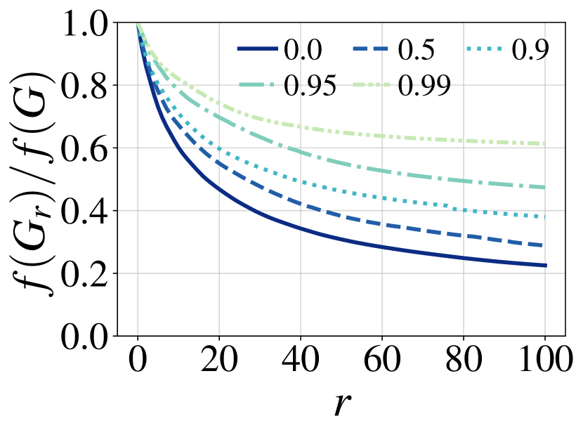
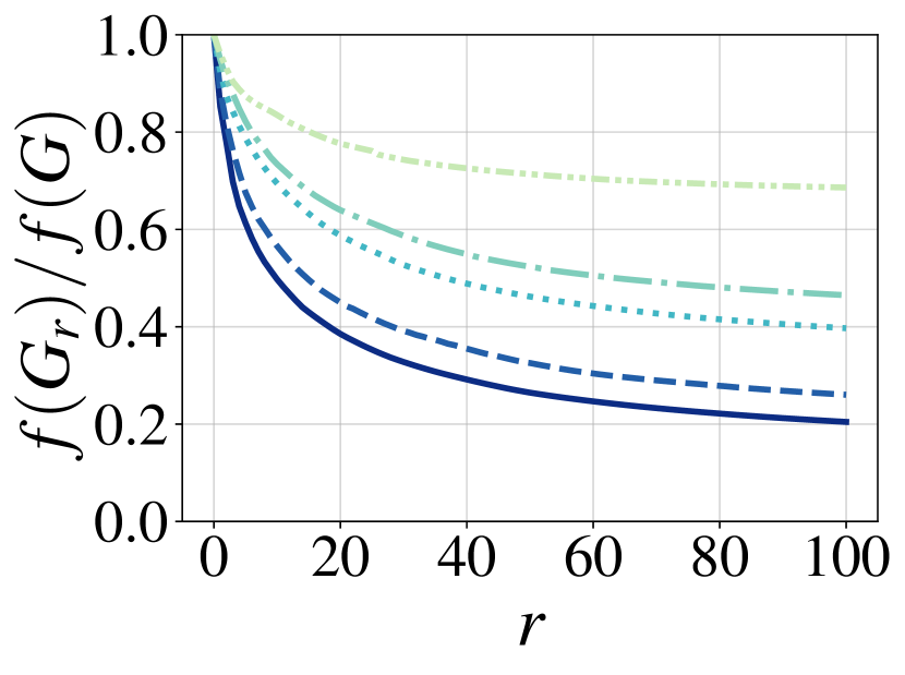
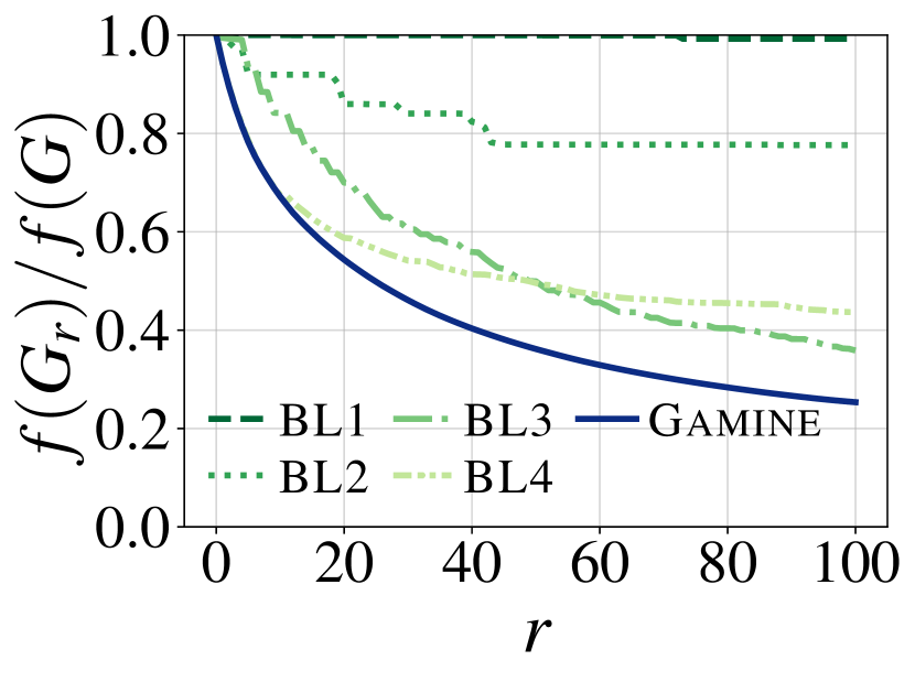
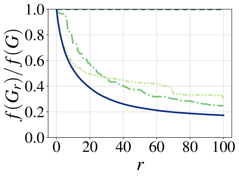
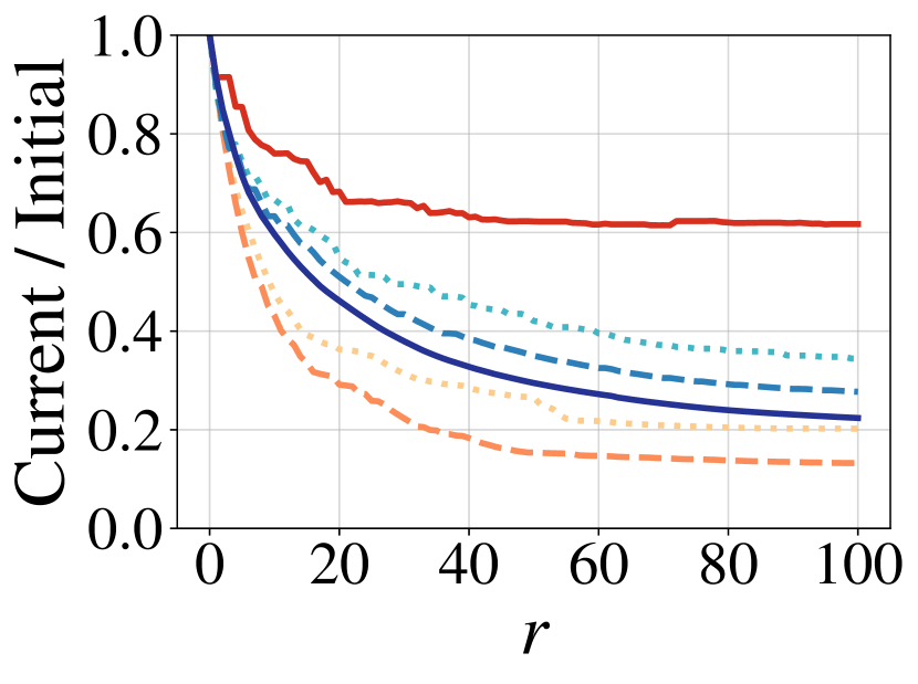
The higher the quality threshold $q$, the more constrained our rewiring options. Thus, under a given budget $r$, we expect Gamine to reduce our objective more strongly for smaller $q$. As illustrated in Fig. 2, our experiments confirm this intuition, and the effect is more pronounced if the out-edge probability distribution is skewed. We further observe that Gamine can guarantee $q=0.5$ with little performance impact, and it can strongly reduce the exposure to harm even under a strict $q=0.95$: With just $100$ edge rewirings, it reduces the expected total exposure to harm by $50\%$, while ensuring that its recommendations are at most $5\%$ less relevant than the original recommendations.

6.2.2. Performance comparisons

Having ensured that Gamine robustly and predictably reduces the total exposure across the entire spectrum of modeling choices, we now compare it with its competitors. Overall, we find that Gamine offers more reliable performance and achieves stronger harm reduction than its contenders.

Comparison with baselines BL1–BL4

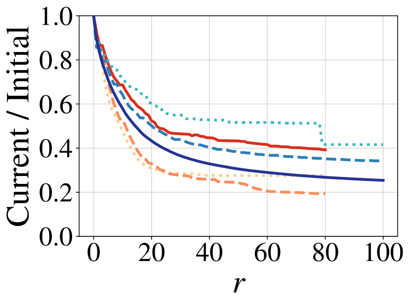
First, we compare Gamine with our four baselines, each representing a different ablation of our algorithm. As depicted in Fig. 3, the general pattern we observe matches our performance expectations (from weak performance of BL1 to strong performance of BL4), but we are struck by the strong performance of BL3 (selecting based on $\sigma$), especially in contrast to the weak performance of BL2 (selecting based on $\tau$). This suggests that whereas the most exposed node does not necessarily have a highly visited node as an in-neighbor, the most visited node tends to have a highly exposed node as an out-neighbor. In other words, for some highly prominent videos, the YouTube algorithm problematically appears to recommend highly harm-inducing content to watch next. Despite the competitive performance of BL3 and BL4, Gamine consistently outperforms these baselines, too, and unlike the baselines, it smoothly reduces the exposure function. This lends additional support to our reliance on $\sigma\tau$ (rewiring a highly visited $i$ away from a highly exposed $j$) as an iteratively evaluated heuristic.

Comparison with MMS

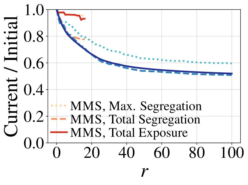
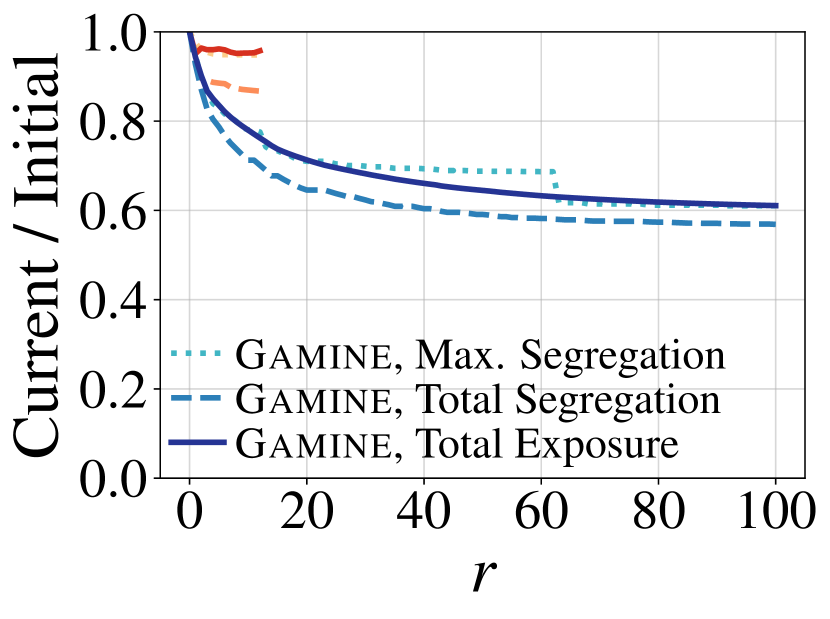
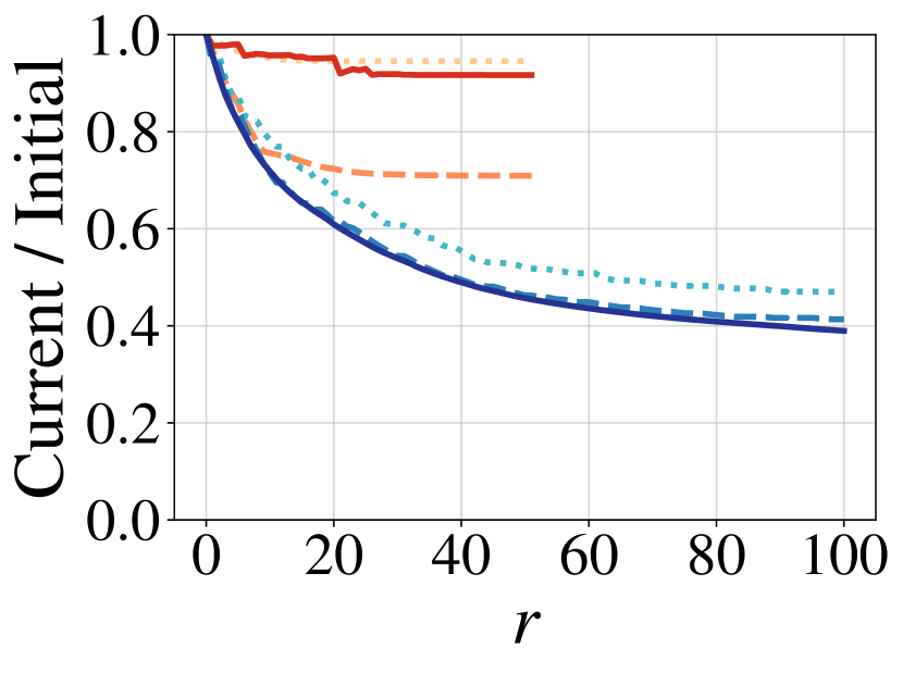
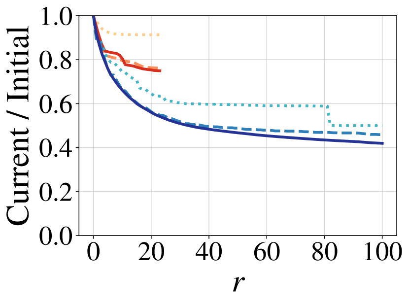
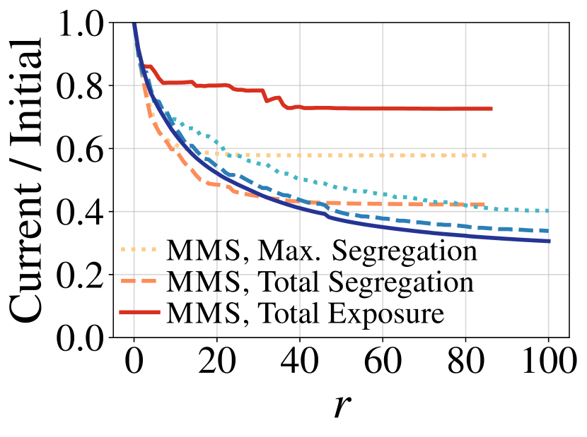
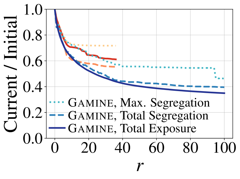
Having established that all components of Gamine are needed to achieve its performance, we now compare our algorithm with MMS, the method proposed by Fabbri et al. (Fabbri et al., 2022). To this end, we run both Gamine and MMS using their respective objective functions, i.e., the expected total exposure to harm of random walks starting at any node (total exposure, Gamine) and the maximum expected number of random-walk steps from a harmful node to a benign node (maximum segregation, MMS). Reporting their performance under the objectives of both algorithms (as well as the total segregation, which sums the segregation scores of all harmful nodes) in Fig. 4, we find that under strict quality control ($q\in\{0.9,0.95,0.99\}$), Gamine outperforms MMS on all objectives, and MMS stops early as it can no longer reduce its objective function. For $q=0.5$, MMS outperforms Gamine on the segregation-based objectives, but Gamine still outperforms MMS on our exposure-based objective, sometimes at twice the margin (Fig. 4(g)). Further, while Gamine delivers consistent and predictable performance that is strong on exposure-based and segregation-based objectives, we observe much less consistency in the performance of MMS. For example, it is counterintuitive that MMS identifies $100$ rewirings on the smaller YT-100k data but stops early on the larger YT-10k data. Moreover, MMS delivers the results shown in Fig. 4 under $c_{B1}$, but it cannot decrease its objective at all on the same data under $c_{B2}$, which differs from $c_{B1}$ only in that it also assigns harm to anti-feminist content (Appendix E, Table 7). We attribute this brittleness to the reliance on the maximum-based segregation objective, which, by design, is less robust than our sum-based exposure objective.

(a) Probability shape $\chi=\mathbf{U}$

(b) Probability shape $\chi=\mathbf{S}$

Figure 2. Performance of Gamine for quality thresholds $q\in\{0.0,0.5,0.9,0.95,0.99\}$ as measured by $c_{B2}$, run on YT-100k with $d=5$ and $\alpha=0.05$. Gamine can ensure $q=0.5$ with little loss in performance, and it can reduce our objective considerably even under a strict $q=0.95$.

(a) Regular out-degree $d=10$

(b) Regular out-degree $d=5$

Figure 3. Performance of Gamine with $q=0.0$, compared with the four baselines BL1, BL2, BL3, and BL4 under $c_{B1}$, run on YT-100k with $\alpha=0.05$ and $\chi=\mathbf{U}$. As BL4 is roundless, we apply its rewirings in decreasing order of $\Delta$ to depict its performance as a function of $r$. Gamine outcompetes all baselines, but BL3 and BL4 also show strong performance.

(a) YT-100k, $q=0.99$

(b) YT-10k, $q=0.99$

(c) YT-100k, $q=0.95$

(d) YT-10k, $q=0.95$

(e) YT-100k, $q=0.9$

(f) YT-10k, $q=0.9$

(g) YT-100k, $q=0.5$

(h) YT-10k, $q=0.5$

Figure 4. Performance of Gamine and MMS when measured under $c_{B1}$ by the maximum segregation or the total segregation from Fabbri et al. (Fabbri et al., 2022), or by the total exposure as defined in Eq. 3, run on YT-100k (left) and YT-10k (right) with $d=5$, $\alpha=0.05$, and $\chi=\mathbf{U}$. For all but $q=0.5$, Gamine outperforms MMS on all objectives, and MMS stops early because it can no longer reduce the maximum segregation.

(a) Gamine on REM

(b) Gamine and MMS on QREM

Figure 5. Scaling of Gamine and MMS under $c_{B1}$ with $\alpha=0.05$, $\chi=\mathbf{U}$, and $q=0.0$ (REM) resp. $0.99$ (QREM). We report the seconds $s$ to compute a single rewiring as a function of $m=dn$ (MMS does not identify any rewirings on NF-Cov19 and NF-All). Gamine scales more favorably than MMS.

6.2.3. Empirical scalability of Gamine

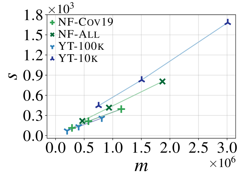
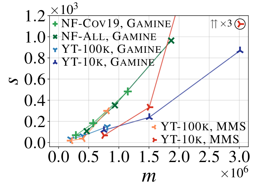
In our previous experiments, we found that Gamine robustly and reliably reduces the expected total exposure to harm. Now, we seek to ascertain that its practical scaling behavior matches our theoretical predictions, i.e., that under realistic assumptions on the input, Gamine scales linearly in $n$ and $m$. We are also interested in comparing Gamine’s scalability to that of MMS. To this end, we measure the time taken to compute a single rewiring and report, in Fig. 5, the average over ten rewirings for each of our datasets. This corresponds to the time taken by 1-REM in Gamine and by 1-Rewiring in MMS, which drives the overall scaling behavior of both algorithms. We find that Gamine scales approximately linearly, whereas MMS scales approximately quadratically (contrasting with the empirical time complexity of $\mathcal{O}(n\log n)$ claimed in (Fabbri et al., 2022)). This is because our implementation of MMS follows the original authors’, whose evaluation of the segregation objective takes time $\mathcal{O}(n)$ and is performed $\mathcal{O}(m)$ times. The speed of precomputations depends on the problem variant (REM vs. QREM), and for QREM, also on the quality function $\theta$. In our experiments, precomputations add linear overhead for Gamine and volatile overhead for MMS, as we report in Section F.2.

6.2.4. Data complexity

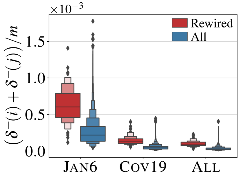
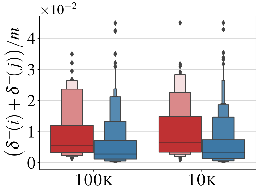
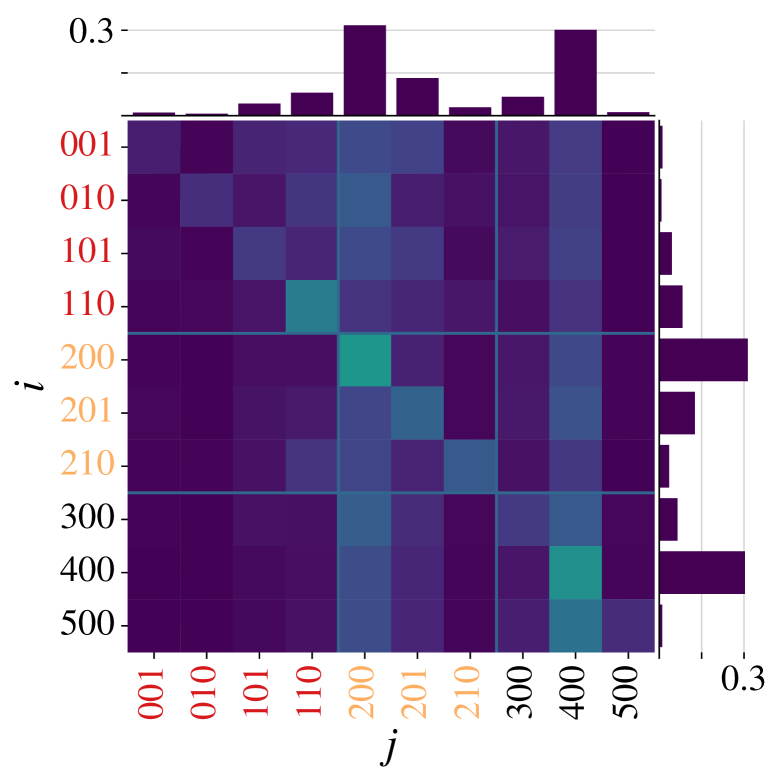
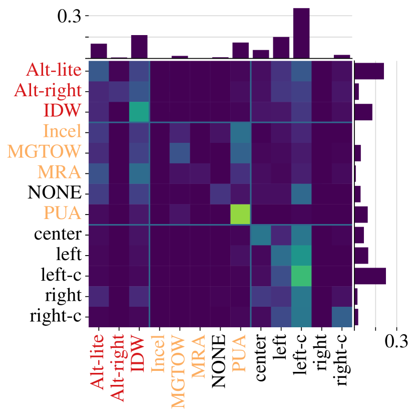
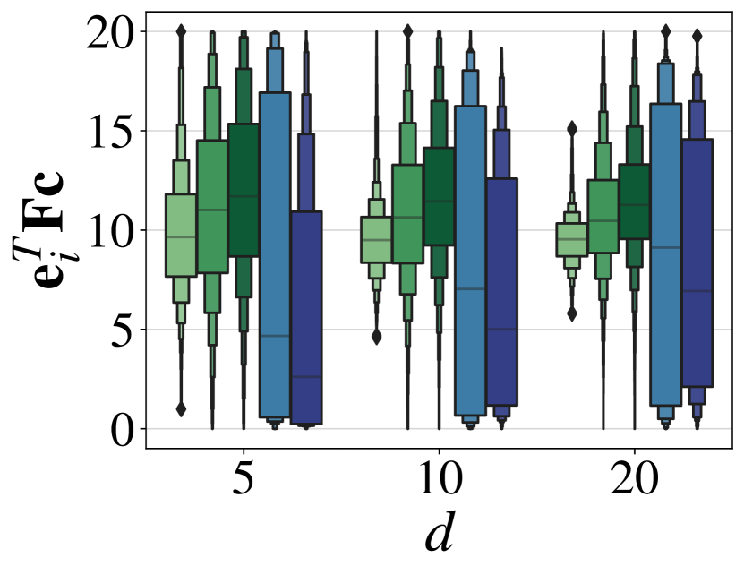
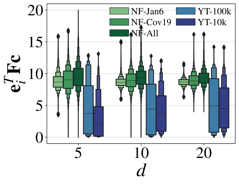
Given that Gamine strongly reduces the expected total exposure to harm with few rewirings on the YouTube data, as evidenced in Figs. 2, 3 and 4, one might be surprised to learn that its performance seems much weaker on the NELA-GT data (Section F.4): While it still reduces the expected total exposure and outperforms MMS (which struggles to reduce its objective at all on the NF data), the impact of individual rewirings is much smaller than on the YouTube datasets, and the value of the quality threshold $q$ barely makes a difference. This motivates us to investigate how data complexity impacts our ability to reduce the expected total exposure to harm via edge rewiring: Could reducing exposure to harm be intrinsically harder on NF data than on YT data? The answer is yes. First, the in-degree distributions of the YT graphs are an order of magnitude more skewed than those of the NF graphs (Section E.2.3, Fig. 15). This is unsurprising given the different origins of their edges (user interactions vs. cosine similarities), but it creates opportunities for high-impact rewirings involving highly prominent nodes in YT graphs (which Gamine seizes in practice, see below). Second, as depicted in Fig. 6, harmful and benign nodes are much more strongly interwoven in the NF data than in the YT data. This means that harmful content is less siloed in the NF graphs, but it also impedes strong reductions of the expected total exposure. Third, as a result of the two previous properties, the initial node exposures are much more concentrated in the NF graphs than in the YT graphs, as illustrated in Fig. 7, with a median sometimes twice as large as the median of the identically parametrized YT graphs, and a much higher average exposure (cf. $\nicefrac{{f(G)}}{{n}}$ in Table 2). Finally, the relevance scores are much more skewed in the YT data than in the NF data (Section E.2.3, Fig. 16). Hence, while we are strongly constrained by $q$ on the YT data even when considering only the $100$ highest-ranked nodes as potential rewiring targets, we are almost unconstrained in the same setting on the NF data, which explains the comparative irrelevance of $q$ on the NF data. Thus, the performance differences we observe between the NF data and the YT data are due to intrinsic dataset properties: REM and QREM are simply more complex on the news data than on the video data.

(a) NF-All

(b) YT-10k

Figure 6. Fractions of edges running between news outlet resp. video channel categories for real-world graphs with $d=5$, with marginals indicating the fraction of sources (right) resp. targets (top) in each category. News outlet categories are denoted as triples (veracity score, conspiracy-pseudoscience flag, questionable-source flag); for video channel categories, $\{\text{left},\text{right}\}$-center is abbreviated as $\{\text{left},\text{right}\}$-c; and label colors are coarse indicators of harm. In NF-All, harmful and benign nodes are more interconnected than in YT-10k.

(a) $c_{B2}$, $\chi=\mathbf{S}$

(b) $c_{R1}$, $\chi=\mathbf{U}$

Figure 7. Distributions of initial node exposures $\mathbf{e}^{T}_{i}\mathbf{F}\mathbf{c}$ in our real-world datasets, computed with $\alpha=0.05$. Note that cost functions sharing a name are defined differently for the YT and NF datasets (based on their semantics). The NF datasets generally exhibit more concentrated exposure distributions than the YT datasets and higher median exposures.

(a) Quality threshold $q=0.0$

(b) Quality threshold $q=0.99$

Figure 8. Channel class of videos in rewirings $(i,j,k)$ on YT-100k with $d=5$, $\alpha=0.05$, and $\chi=\mathbf{U}$, computed using $c_{R1}$, for different quality thresholds. Rewirings between classes are color-scaled by their count, using blues if $c_{R1}(k)<c_{R1}(j)$, reds if $c_{R1}(k)>c_{R1}(j)$, and grays otherwise. For $q=0.0$, we only replace costly targets $j$ by less costly targets $k$, as expected, but for $q=0.99$, we see many rewirings with $c_{R1}(k)\geq c_{R1}(j)$.

(a) YT-100k

(b) YT-10k

Figure 9. Mapping the nodes in each rewiring $(i,j,k)$ to their costs $(c_{i},c_{j},c_{k})$, we report the fraction of rewirings in each cost class under $c_{B1}$ and $q\in\{0.0,0.5,0.9,0.95,0.99\}$, for YT graphs with $d=5$, $\alpha=0.05$, and $\chi=\textbf{U}$. While most intuitively suboptimal classes occur rarely (e.g., 001, 011, 101), under quality constraints, we often rewire among harmful nodes.

6.2.5. General guidelines

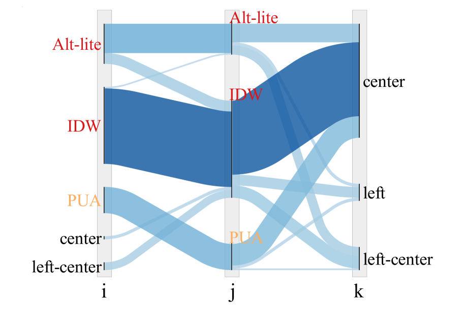
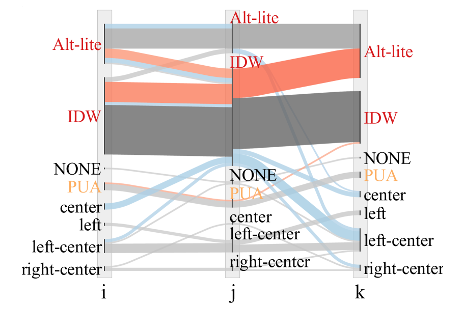
Finally, we would like to abstract the findings from our experiments into general guidelines for reducing exposure to harm in recommendation graphs, especially under quality constraints. To this end, we analyze the metadata associated with our rewirings. In particular, for each set of rewirings $(i,j,k)$ obtained in our experiments, we are interested in the channel resp. news outlet classes involved, as well as in the distributions of cost triples $(c_{i},c_{j},c_{k})$ and in-degree tuples $(\delta^{-}\!(i),\delta^{-}\!(j))$. As exemplified in Fig. 8, while we consistently rewire edges from harmful to benign targets in the quality-unconstrained setting ($q=0.0$), under strict quality control ($q=0.99$), we frequently see rewirings from harmful to equally or more harmful targets. More generally, as illustrated in Fig. 9, the larger the threshold $q$, the more we rewire among harmful, resp. benign, nodes ($c_{i}=c_{j}=c_{k}=1$, resp. $0$)—which MMS does not even allow. Furthermore, the edges we rewire typically connect nodes with large in-degrees (Section F.5, Fig. 28). We conclude that a simplified strategy for reducing exposure to harm under quality constraints is to identify edges that connect high-cost nodes with large in-degrees, and rewire them to the node with the lowest exposure among all nodes meeting the quality constraints.

7. Discussion and Conclusion

We studied the problem of reducing the exposure to harmful content in recommendation graphs by edge rewiring. Modeling this exposure via absorbing random walks, we introduced QREM and REM as formalizations of the problem with and without quality constraints on recommendations. We proved that both problems are NP-hard and NP-hard to approximate to within an additive error, but that under mild assumptions, the greedy method provides a $(1-\nicefrac{{1}}{{e}})$-approximation for the REM problem. Hence, we introduced Gamine, a greedy algorithm for REM and QREM running in linear time under realistic assumptions on the input, and we confirmed its effectiveness, robustness, and efficiency through extensive experiments on synthetic data as well as on real-world data from video recommendation and news feed applications.

Our work improves over the state of the art (MMS by Fabbri et al. (Fabbri et al., 2022)) in terms of performance, and it eliminates several limitations of prior work. While Fabbri et al. (Fabbri et al., 2022) model benign nodes as absorbing states and consider a brittle max-objective that is minimized even by highly harm-exposing recommendation graphs, we model benign nodes as transient states and consider a robust sum-objective that captures the overall consumption of harmful content by users starting at any node in the graph. Whereas MMS can only handle binary node labels, Gamine works with real-valued node attributes, which permits a more nuanced encoding of harmfulness.

We see potential for future work in several directions. For example, it would be interesting to adapt our objective to mitigate polarization, i.e., the separation of content with opposing views, with positions modeled as positive and negative node costs. Moreover, we currently assume that all nodes are equally likely as starting points of random walks, which is unrealistic in many applications. Finally, we observe that harm reduction in recommendation graphs has largely been studied in separation from harm reduction in other graphs representing consumption phenomena, such as user interaction graphs. A framework for optimizing functions under budget constraints that includes edge rewirings, insertions, and deletions could unify these research lines and facilitate future progress.

ethicsmark.sectionethicsmark.sectionEthics StatementEthics Statementethicsmark.section

Ethics Statement

In this work, we introduce Gamine, a method to reduce the exposure to harm induced by recommendation algorithms on digital media platforms via edge rewiring, i.e., replacing certain recommendations by others. While removing harm-inducing recommendations constitutes a milder intervention than censoring content directly, it still steers attention away from certain content to other content, which, if pushed to the extreme, can have censorship-like effects. Although in its intended usage, Gamine primarily counteracts the tendency of recommendation algorithms to overexpose harmful content as similar to other harmful content, when fed with a contrived cost function, it could also be used to discriminate against content considered undesirable for problematic reasons (e.g., due to political biases or stereotypes against minorities). However, as the changes to recommendations suggested by Gamine could also be made by amending recommendation algorithms directly, the risk of intentional abuse is no greater than that inherent in the recommendation algorithms themselves, and unintentional abuse can be prevented by rigorous impact assessments and cost function audits before and during deployment. Thus, we are confident that overall, Gamine can contribute to the health of digital platforms.

appendixmark.sectionappendixmark.sectionAppendixAppendixappendixmark.section

Appendix

In addition to Table 3, included below, the written appendix to this work contains the following sections:

1. Omitted proofs

2. Other graph edits

3. Omitted pseudocode

4. Reproducibility information

5. Dataset information

6. Further experiments

This appendix, along with the main paper, is available on arXiv and also deposited at the following DOI: 10.5281/zenodo.8002980. To facilitate reproducibility, all code, data, and results are made available at the following DOI: 10.5281/zenodo.7936816.

Table 3. Most important notation used in this work.

notationmark.sectionnotationmark.sectionNotationNotationnotationmark.section Symbol Definition Description Graph Notation $G$ $=$ $(V,E)$ Graph $n$ $=$ $|V|$ Number of nodes $m$ $=$ $|E|$ Number of edges $\delta^{-}\!(i)$ $=$ $|\{j\mid(j,i)\in E\}|$ In-degree of node $i$ $\Gamma^{+}\!(i)$ $=$ $\{j\mid(i,j)\in E\}$ Set of out-neighbors of node $i$ $\delta^{+}\!(i)$ $=$ $|\Gamma^{+}\!(i)|$ Out-degree of node $i$ $d$ Regular out-degree of an out-regular graph $\Delta^{+}$ $=$ $\max\{\delta^{+}\!(i)\mid i\in V\}$ Maximum out-degree $S$ $=$ $\{i\in V\mid\mathbf{e}_{i}^{T}\mathbf{F}\mathbf{c}=0\}$ Set of safe nodes $U$ $=$ $\{i\in V\mid\mathbf{e}_{i}^{T}\mathbf{F}\mathbf{c}>0\}$ Set of unsafe nodes $\Lambda^{+}$ $=$ $\max\{\delta^{+}\!(i)\mid i\in U\}$ Maximum out-degree of an unsafe node Matrix Notation $\mathbf{M}[i,j]$ Element in row $i$, column $j$ of $\mathbf{M}$ $\mathbf{M}[i,:]$ Row $i$ of $\mathbf{M}$ $\mathbf{M}[:,j]$ Column $j$ of $\mathbf{M}$ $\mathbf{e}_{i}$ $i$-th unit vector $\mathbf{1}$ All-ones vector $\mathbf{I}$ Identity matrix $\lVert\mathbf{M}\rVert_{\infty}$ $=$ $\max_{i}\sum_{j=0}^{n}\mathbf{M}[i,j]$ Infinity norm Notation for REM and QREM $(i,j,k)$ Rewiring replacing $(i,j)\in E$ by $(i,k)\notin E$ with $p_{ik}=p_{ij}$, cf. Table 1 $r$ $\in$ $\mathbb{N}$ Rewiring budget $\alpha$ $\in$ $(0,1]$ Random-walk absorption probability $p_{ij}$ $\in$ $(0,1-\alpha]$ Probability of traversing $(i,j)$ from $i$ $\mathbf{P}$ $\in$ $[0,1-\alpha]^{n\times n}$ Random-walk transition matrix $\mathbf{F}$ $=$ $\sum_{i=0}^{\infty}\mathbf{P}^{i}=(\mathbf{I}-\mathbf{P})^{-1}$ Fundamental matrix $c$ Cost function with range $[0,1]$ $c_{i}$ $\in$ $[0,1]$ Cost associated with node $i$ $\mathbf{c}$ $\in$ $[0,1]^{n}$ Vector of node costs $\kappa$ $\in$ $\mathbb{N}$ Number of power iterations $\chi$ $\in$ $\{\mathbf{U},\mathbf{S}\}$ Shape of probability distribution over the out-edges of a node Notation for QREM Only $\mathbf{R}$ $\in$ $\mathbb{R}_{\geq 0}^{n\times n}$ Relevance matrix $\theta$ Relevance function with range $[0,1]$ $q$ $\in$ $[0,1]$ Quality threshold $\mathbf{r}_{i}$ $\in$ $V^{\delta^{+}\!(i)}$ Relevance-ordered targets of out-edges of $i$ $\text{idx}_{i}(j)$ Relevance rank of node $j$ for node $i$ $T_{\delta^{+}}\!(i)$ $=$ $\{j\mid\text{idx}_{i}(j)\leq\delta^{+}\!(i)\}$ Set of the $\delta^{+}\!(i)$ nodes most relevant for node $i$ DCG $=$ $\sum_{j\in\Gamma^{+}\!(i)}\frac{\mathbf{R}[i,j]}{\log_{2}(1+\text{idx}_{i}(j))}$ Discounted Cumulative Gain iDCG $=$ $\sum_{j\in T_{\delta^{+}}\!(i)}\frac{\mathbf{R}[i,j]}{\log_{2}(1+\text{idx}_{i}(j))}$ Ideal Discounted Cumulative Gain nDCG $=$ $\frac{\textsc{DCG}(i)}{\textsc{iDCG}(i)}$ Normalized Discounted Cumulative Gain Notation Related to the Exposure Function $f$ and its Analysis $f(G)$ $=$ $\mathbf{1}^{T}\mathbf{F}c$ Exposure function (minimization objective) $f_{\Delta}(G,G_{r})$ $=$ $f(G)-f(G_{r})$ Reduction-in-exposure function (equivalent maximization objective) $G^{\prime}$, $\mathbf{P}^{\prime}$, $\mathbf{F}^{\prime}$ Graph $G$, transition matrix $\mathbf{P}$, fundamental matrix $\mathbf{F}$, as updated by rewiring $(i,j,k)$, cf. Table 1 $\mathbf{u}$ $=$ $p_{ij}\mathbf{e}_{i}$ Vector capturing the source $i$ of a rewiring $(i,j,k)$ and the traversal probability of $(i,j)$ $\mathbf{v}$ $=$ $\mathbf{e}_{j}-\mathbf{e}_{k}$ Vector capturing the old target $j$ and the new target $k$ of a rewiring $(i,j,k)$ $\sigma$ $=$ $\mathbf{1}^{T}\mathbf{F}\mathbf{u}$ $p_{ij}$-scaled $i$-th column sum $\tau$ $=$ $\mathbf{v}^{T}\mathbf{F}\mathbf{c}$ $\mathbf{c}$-scaled sum of differences between the $j$-th row sum and the $k$-th row sum $\rho$ $=$ $1+\mathbf{v}^{T}\mathbf{F}\mathbf{u}$ Normalization factor ensuring that $\mathbf{F}^{\prime}\mathbf{1}=\mathbf{F}\mathbf{1}$ $\Delta$ $=$ $f_{\Delta}(G,G^{\prime})=\nicefrac{{\sigma\tau}}{{\rho}}$ Reduction of $f$ obtained by a single rewiring $(i,j,k)$ $\hat{\Delta}$ $=$ $\Delta\rho=\sigma\tau$ Heuristic for $\Delta$

Appendix

In this appendix, we present the proofs omitted in the main paper (Appendix A), discuss alternative graph edit operations (Appendix B), and state the pseudocode for Gamine as well as the algorithms leading up to it (Appendix C). We also provide further reproducibility information (Appendix D), more details on our datasets (Appendix E), and additional experimental results (Appendix F).

Appendix A Omitted Proofs

In this section, we provide the full proofs of our hardness results for REM, which carry over to QREM: NP-hardness (1) and hardness of approximation (2). We further give the complete proofs of the submodularity of $f_{\Delta}$ (1 and 3) and of the mathematical structure in $\Delta$ (2).

A.1. NP-Hardness of REM

See 1

Proof.

We reduce from minimum vertex cover for undirected cubic, i.e., 3-regular graphs (MVC-3), which is known to be NP-hard (Greenlaw and Petreschi, 1995). To this end, we transform an instance of MVC-3 into an instance of REM with a directed, 3-out-regular input graph (REM-3 instance) as follows. From a cubic undirected graph $G^{\prime}=(V^{\prime},E^{\prime})$ with $n^{\prime}=|V^{\prime}|$ and $m^{\prime}=|E^{\prime}|=\nicefrac{{3n^{\prime}}}{{2}}$, we construct our directed REM-3 instance by defining a graph $G=(V,E)$ with $n=|V|=2n^{\prime}+4$ nodes and $m=|E|=6n^{\prime}+12$ edges such that

$$V=~{} V^{\prime}\cup\overline{V^{\prime}}\cup S\;,~{}\text{for}~{}\overline{V^{\prime}}=\{b_{i}\mid i\in V^{\prime}\}\;,~{}S=\{g_{1},g_{2},g_{3},g_{4}\}\;,$$

$$E=~{} \{(i,b_{i})\mid i\in V^{\prime}\}\cup\{(b_{i},j)\mid\{i,j\}\in E^{\prime}\}$$

$$\cup\{(g_{i},g_{j})\in S\times S\mid i\neq j\}\cup\{(i,g_{x})\mid i\in V^{\prime},x\in\{1,2\}\}\;,$$

$$\mathbf{P}[x,y]=~{} \frac{1-\alpha}{\delta^{+}\!(x)}=\frac{1-\alpha}{3}\;,~{}\text{and}~{}c_{x}=\begin{cases}1&x\in\overline{V^{\prime}}\\ 0&\text{otherwise}\;.\end{cases}$$

That is, for each node $i\in V^{\prime}$, we introduce a node $i\in V$ with $c_{i}=0$, a companion node $b_{i}\in V$ with $c_{b_{i}}=1$, and an edge $(i,b_{i})\in E$ in $G$. We then encode the original edge set implicitly by defining two edges $(b_{i},j)\in E$ and $(b_{j},i)\in E$ for each edge $\{i,j\}\in E^{\prime}$. Finally, we add a complete 3-out-regular graph of zero-cost nodes and connect each node representing a node from $V^{\prime}$ to the first two nodes of that graph.

Intuitively, the edges $\{(i,b_{i})\mid i\in V^{\prime}\}$ will be our prime candidates for rewiring—and rewiring an edge $(i,b_{i})$ in REM-3 will correspond to selecting node $i$ into the vertex cover of the original MVC-3 instance. The implicit encoding of the original edge set introduces the asymmetry necessary to tell from the value of our objective function if an optimal $r$-rewiring of $G$ corresponds to a vertex cover of cardinality $r$ in $G^{\prime}$. Adding a complete 3-out-regular graph of zero-cost nodes gives us a strongly connected safe component $S$ of nodes as rewiring targets, and it ensures that $G$ is 3-out-regular. The entire transformation is visualized in Fig. 10.

(a) Toy MVC-3 instance $G^{\prime}=(V^{\prime},E^{\prime})$

(b) REM-3 instance constructed from $G^{\prime}$

Figure 10. Reduction setup for 1. Fig. 10(a) depicts a toy MVC-3 instance, which we transform into a REM-3 instance as shown in Fig. 10(b). In Fig. 10(b), white nodes represent $V^{\prime}$, gray nodes represent $\overline{V^{\prime}}$, silver nodes represent $S$, and edges $ab$ with $c_{a}=0$ and $c_{b}=1$ are drawn in red. Silver edges and nodes with silver boundaries are needed to ensure that $G$ is 3-out-regular, and all edges are traversed with probability $\frac{(1-\alpha)}{3}$.

In the graph $G$ thus constructed, the only nodes ever exposed to harm are the $n^{\prime}$ nodes in $V^{\prime}$ and the $n^{\prime}$ nodes in $\overline{V^{\prime}}$. As illustrated in Fig. 11, random walks starting from a node in $\overline{V^{\prime}}$ only see nodes with cost $1$ after an even number of steps, random walks starting from a node in $V^{\prime}$ only see nodes with cost $1$ after an odd number of steps, and as $G$ is 3-out-regular, all random walks have a branching factor of $3$, such that they see exactly $3^{t}$ (not necessarily distinct) nodes at $t$ steps from their origin. Each node in $V^{\prime}$ has three out-neighbors, and before the first rewiring, exactly one of them is a node with cost $1$. Thus if the random walks do not get absorbed, the regularity in our construction implies that the probability of encountering a node with cost $1$ after $2$ steps from a node in $\overline{V^{\prime}}$ is $\frac{3^{1}}{3^{2}}=\frac{1}{3}$, just like the probability of encountering a node with cost $1$ after $3$ steps from a node in $V^{\prime}$ is $\frac{3^{1}}{3^{3}}=\frac{1}{9}$. Therefore, the starting value of our objective function can be written succinctly as

(12) $$f(G)=\underbrace{n^{\prime}\sum_{t=0}^{\infty}3^{-t}(1-\alpha)^{2t}}_{\text{Contributions from $\overline{V^{\prime}}$}}+\underbrace{n^{\prime}\sum_{t=0}^{\infty}3^{-t-1}(1-\alpha)^{2t+1}}_{\text{Contributions from $V^{\prime}$}}\;.$$

(a) Walks starting at node $i\in V^{\prime}$

(b) Walks starting at node $b_{i}\in\overline{V^{\prime}}$ (safe nodes at step $4$ not shown)

Figure 11. Random walks in 3-out-regular directed graphs $G=(V,E)$ constructed from undirected MVC-3 instances as depicted in Fig. 10. All edges are traversed with probability $\frac{1-\alpha}{3}$, nodes in $\overline{V^{\prime}}$ are drawn in gray, and branches leading into the safe component $S$ are collated into silver square boxes labeled $S$. The annotations at level $t$ to the right of each random-walk tree indicate the fraction of nodes with cost $1$ of all nodes encountered after taking exactly $t$ steps.

Since $S$ contains four safe nodes and $G$ is 3-out-regular, we can always rewire edges with unsafe targets to safe targets without creating multi-edges. Therefore, as long as $r\leq n^{\prime}$, an optimal rewiring $X$ will contain triples of shape $(i,b_{i},g_{x})$, where $g_{x}$ is any node that is safe after the $r$ rewirings have been performed (this includes the nodes in $S$ but can also include other zero-cost nodes $i$ for which $(i,b_{i},g_{x^{\prime}})$ is part of the rewiring for some other, safe node $g_{x^{\prime}}$). Now, each individual rewiring reduces the objective by

(13) $$\underbrace{\frac{1}{3}(1-\alpha)}_{(1)}+\underbrace{\frac{3}{9}(1-\alpha)^{2}}_{(2)}+\underbrace{\frac{2\gamma^{\prime}}{27}(1-\alpha)^{3}}_{(3)}+~{}\varepsilon^{\prime}\;,$$

where $\varepsilon^{\prime}$ is a term summarizing all contributions from walks longer than $3$ steps, and $\gamma^{\prime}$ is the number of edges that are newly covered in $G^{\prime}$ by selecting the source node $i$ of our rewiring in $G$ into the vertex cover $C$ of $G^{\prime}$, i.e.,

(14) $$\gamma^{\prime}=|\{e\in E^{\prime}\mid C\cap e=\emptyset\}|~{}~{}\text{for}~{}~{}C=\{i\in V^{\prime}\mid(i,b_{i})\in E_{X}\}\;,$$

where $E_{X}$ is the set of previously rewired edges in $G$.

More elaborately, in Eq. 13, the component marked (1) is the exposure of $i$ to $b_{i}$ at distance $1$ via the walk $(i,b_{i})$, and the component marked (2) is the exposure of $b_{j}$ to $b_{i}$ at distance $2$ via the walk $(b_{j},i,b_{i})$, for the three nodes $j$ such that $\{i,j\}\in E^{\prime}$, where $|\{\{x,y\}\in E^{\prime}\mid y=j\}|=3$ because $G^{\prime}$ is 3-regular. The component marked (3) is the sum of (i) the exposure of $i$ to nodes $b_{j}$ with $\{i,j\}\in E^{\prime}$ at distance $3$ via the walk $(i,b_{i},j,b_{j})$, and (ii) the exposure of nodes $j$ with $\{i,j\}\in E^{\prime}$ to node $i$ at distance $3$ via the walk $(j,b_{j},i,b_{i})$, each of which is

$$\frac{1}{27}(1-\alpha)^{3}\cdot(1-|E_{X}\cap\{(j,b_{j})\}|)=\begin{cases}\frac{1}{27}(1-\alpha)^{3}&\text{if}~{}(j,b_{j})\notin E_{X}\\ 0&\text{otherwise}\;.\end{cases}$$

Hence, the objective function reduces by $\frac{2}{27}(1-\alpha)^{3}$ for each edge $\{i,j\}\in E^{\prime}$ that is covered for the first time when we select $i$ into the vertex cover of $G^{\prime}$, and because $G^{\prime}$ is 3-regular, each rewiring can cover at most 3 new edges, such that $\gamma^{\prime}\leq 3$.

Thus, an optimal $r$-rewiring of $G$ reduces the objective function in Eq. 12 by

(15) $$f_{\Delta}(G,G_{r})=\frac{r}{3}(1-\alpha)+\frac{3r}{9}(1-\alpha)^{2}+\frac{2\gamma}{27}(1-\alpha)^{3}+\varepsilon\;,$$

where $\gamma\geq\frac{3}{2}r$ is the number of edges in $G^{\prime}$ that are covered by the source nodes of our rewirings, and $\varepsilon$ is the sum of the small terms $\varepsilon^{\prime}$ associated with each rewiring. Therefore, $G^{\prime}$ has a minimum vertex cover of size at most $r$ if and only if an optimal $r$-rewiring of $G$ reduces our objective by

(16) $$f_{\Delta}(G,G_{r})=\frac{r}{3}(1-\alpha)+\frac{3r}{9}(1-\alpha)^{2}+\frac{2m^{\prime}}{27}(1-\alpha)^{3}+\varepsilon\;,$$

i.e., $G^{\prime}$ has a minimum vertex cover of size at most $r$ if and only if

$$f(G_{r})=~{} f(G)-f_{\Delta}(G,G_{r})$$

$$=~{} n^{\prime}+\frac{n^{\prime}-r}{3}(1-\alpha)+\frac{3(n^{\prime}-r)}{9}(1-\alpha)^{2}+\frac{3n^{\prime}-2m^{\prime}}{27}(1-\alpha)^{3}$$

$$+(\xi-\varepsilon)$$

$$=~{} n^{\prime}+\frac{n^{\prime}-r}{3}(1-\alpha)+\frac{3(n^{\prime}-r)}{9}(1-\alpha)^{2}+\frac{3n^{\prime}-2\frac{3n^{\prime}}{2}}{27}(1-\alpha)^{3}$$

$$+(\xi-\varepsilon)$$

(17) $$=~{} n^{\prime}+\frac{n^{\prime}-r}{3}(1-\alpha)+\frac{3(n^{\prime}-r)}{9}(1-\alpha)^{2}+(\xi-\varepsilon)\;,$$

where $\xi\geq\varepsilon$ is the entire exposure of random walks in $G$ due to nodes encountered after four or more steps, i.e.,

(18) $$\xi =\underbrace{n^{\prime}\sum_{t=0}^{\infty}3^{-t}(1-\alpha)^{2t}}_{\text{\emph{All} contributions from $\overline{V^{\prime}}$}}+\underbrace{n^{\prime}\sum_{t=0}^{\infty}3^{-t-1}(1-\alpha)^{2t+1}}_{\text{\emph{All} contributions from $V^{\prime}$}}$$

$$\quad-\underbrace{n^{\prime}\sum_{t=0}^{1}3^{-t}(1-\alpha)^{2t}}_{\text{At most $3$ steps from $\overline{V^{\prime}}$}}-\underbrace{n^{\prime}\sum_{t=0}^{1}3^{-t-1}(1-\alpha)^{2t+1}}_{\text{At most $3$ steps from $V^{\prime}$}}\;.$$

As we do not know $\varepsilon$ exactly, we cannot check Eq. 17 directly to decide whether $G^{\prime}$ has a vertex cover of size at most $r$. Instead, we would like to check if

(19) $$f_{\Delta}(G,G_{r})\geq\frac{r}{3}(1-\alpha)+\frac{3r}{9}(1-\alpha)^{2}+\frac{2m^{\prime}}{27}(1-\alpha)^{3}\;,$$

that is, for the purposes of our decision, we would like to ignore $\varepsilon$. Observe that as $\varepsilon\leq\xi$, we can safely do this if

(20) $$\xi<\frac{2}{27}(1-\alpha)^{3}\;,$$

as in this case, the entire exposure of random walks due to nodes encountered after four or more steps in $G$ is smaller than the change of the objective function we obtain by covering a single new edge in the original MVC-3 instance $G^{\prime}$. In 3, we prove that if we choose $\alpha\geq\frac{1}{2}$, then Eq. 20 is guaranteed. Hence, $G^{\prime}$ has a minimum vertex cover of size at most $r$ if and only if Eq. 19 holds, and we obtain the vertex cover of $G^{\prime}$ by setting

$$C=\{i\in V^{\prime}\mid(i,b_{i})\in E_{X}\}\;.$$

∎

Lemma 3.

If in the setting of 1, we set the random-walk absorption probability to $\alpha\geq\frac{1}{2}$, then $\xi<\frac{2}{27}(1-\alpha)^{3}$.

Proof.

Recall the definition of $\xi$ from Eq. 18, and observe that the infinite series involved have closed-form solutions

$$\sum_{t=0}^{\infty}3^{-t}(1-\alpha)^{2t}=\sum_{t=0}^{\infty}\frac{(1-\alpha)^{2t}}{3^{t}}=\sum_{t=0}^{\infty}\bigg{(}\frac{(1-\alpha)^{2}}{3}\bigg{)}^{t}$$

$$=\frac{1}{1-\frac{(1-\alpha)^{2}}{3}}\;,~{}\text{and}$$

$$\sum_{t=0}^{\infty}3^{-t-1}(1-\alpha)^{2t+1}=\sum_{t=0}^{\infty}\frac{(1-\alpha)^{2t+1}}{3^{t+1}}=\sum_{t=0}^{\infty}\frac{1-\alpha}{3}\bigg{(}\frac{(1-\alpha)^{2}}{3}\bigg{)}^{t}$$

$$=\frac{\frac{1-\alpha}{3}}{1-\frac{(1-\alpha)^{2}}{3}}\;,$$

and that the partial sums evaluate to

$$\sum_{t=0}^{1}3^{-t}(1-\alpha)^{2t}=1+\frac{1}{3}(1-\alpha)^{2}\;,~{}\text{and}$$

$$\sum_{t=0}^{1}3^{-t-1}(1-\alpha)^{2t+1}=\frac{1}{3}(1-\alpha)+\frac{1}{9}(1-\alpha)^{3}\;.$$

Using these equalities to rewrite Eq. 18 for $\xi$, and intermittently setting $x=1-\alpha$, where for $\alpha\geq\frac{1}{2}$, we have $x\leq\frac{1}{2}$, we obtain

$$\xi =\frac{1+\frac{(1-\alpha)}{3}}{1-\frac{(1-\alpha)^{2}}{3}}-1-\frac{(1-\alpha)^{2}}{3}-\frac{(1-\alpha)}{3}-\frac{(1-\alpha)^{3}}{9}$$

$$=\frac{1+\frac{x}{3}}{1-\frac{x^{2}}{3}}-1-\frac{x^{2}}{3}-\frac{x}{3}-\frac{x^{3}}{9}$$

$$=\frac{1+\frac{x}{3}}{1-\frac{x^{2}}{3}}-\frac{1-\frac{x^{2}}{3}}{1-\frac{x^{2}}{3}}-\frac{\frac{x^{2}}{3}-\frac{x^{2}}{3}\frac{x^{2}}{3}}{1-\frac{x^{2}}{3}}-\frac{\frac{x}{3}-\frac{x}{3}\frac{x^{2}}{3}}{1-\frac{x^{2}}{3}}-\frac{\frac{x^{3}}{9}-\frac{x^{3}}{9}\frac{x^{2}}{3}}{1-\frac{x^{2}}{3}}$$

$$=\frac{1+\frac{x}{3}-1+\frac{x^{2}}{3}-\frac{x^{2}}{3}+\frac{x^{2}}{3}\frac{x^{2}}{3}-\frac{x}{3}+\frac{x}{3}\frac{x^{2}}{3}-\frac{x^{3}}{9}+\frac{x^{3}}{9}\frac{x^{2}}{3}}{1-\frac{x^{2}}{3}}$$

$$=\frac{\frac{x^{4}}{9}+\frac{x^{5}}{27}}{1-\frac{x^{2}}{3}}=\frac{\frac{x}{9}+\frac{x^{2}}{27}}{1-\frac{x^{2}}{3}}x^{3}$$

$$\leq\frac{\frac{1}{18}+\frac{1}{108}}{1-\frac{1}{12}}x^{3}=\frac{108+18}{18\cdot 108}\cdot\frac{12}{11}x^{3}$$

$$=\frac{126}{3\cdot 54\cdot 11}x^{3}=\frac{126}{1\,749}x^{3}=\frac{3\,402}{1\,749\cdot 27}x^{3}$$

$$<\frac{3\,498}{1\,749\cdot 27}x^{3}=\frac{2}{27}x^{3}=\frac{2}{27}(1-\alpha)^{3}\;,$$

as required. ∎

Note that the choice of $\alpha\geq\frac{1}{2}$ in 3 is almost tight, as for $\alpha=1-\frac{1}{10}(\sqrt{201}-9)\approx 0.48$, we have

(21) $$\frac{\frac{1-\alpha}{9}+\frac{(1-\alpha)^{2}}{27}}{1-\frac{(1-\alpha)^{2}}{3}}=\frac{2}{27}\;.$$

We present the slightly looser bound as it suffices to prove 1 and simplifies the presentation.

A.2. Hardness of Approximation for REM

See 2

Proof.

Under the UGC, MVC is hard to approximate to within a factor of $(2-\varepsilon)$ (Khot and Regev, 2008), and it is generally hardest to approximate on regular graphs (Feige, 2003). Therefore, consider again the reduction construction from the proof of 1 with an original MVC-3 graph $G^{\prime}=(V^{\prime},E^{\prime})$ as well as a transformed REM graph $G=(V,E)$, and assume that $\alpha=\frac{1}{2}$, satisfying 3.

A solution to REM on a graph derived from an MVC-3 instance that has a minimum vertex cover of size $r$ which approximates the optimum to within an additive error of

(22) $$\frac{2r}{27}(1-\alpha)^{3}-\frac{2\frac{r-\varepsilon r}{2}}{27}(1-\alpha)^{3}=\frac{(1+\varepsilon)r}{27}(1-\alpha)^{3}=\frac{(1+\varepsilon)r}{27\cdot 8}$$

would rewire edges such that $\frac{r-\varepsilon r}{2}$ edges in the MVC-3 instance remain uncovered. In this case, taking both endpoints of all uncovered edges yields a vertex cover of size $r+2\frac{r-\varepsilon r}{2}=(2-\varepsilon)r$. Thus, if there existed an algorithm $\mathcal{A}$ discovering the stated approximate solution to REM in polynomial time, we could obtain a $(2-\varepsilon)$-approximation to MVC-3 in polynomial time by transforming the MVC-3 instance into a REM-3 instance, running $\mathcal{A}$ for all integers $r\in\{\frac{n^{\prime}}{4},\dots,\frac{2n^{\prime}}{3}\}$, where $\frac{n^{\prime}}{4}$ and $\frac{2n^{\prime}}{3}$ are the minimum resp. maximum cardinality of an MVC on a 3-regular undirected graph with $n^{\prime}$ nodes, reconstructing the vertex cover solutions, and finally picking the solution with the smallest cardinality. This would contradict the UGC. Observing that the cardinality of an MVC in 3-regular undirected graphs with $n^{\prime}$ nodes is in $r\in\Theta(n^{\prime})$, that $n^{\prime}\in\Theta(n)$, and that $\frac{(1+\varepsilon)}{27\cdot 8}\in\Theta(1)$, the claim follows. ∎

A.3. Submodularity of $f_{\Delta}$

See 1

Proof.

By assumption, there exists a safe node in $G$. Therefore, fix a safe node $s$, and observe that $s$ is an optimal rewiring target because $\mathbf{e}_{s}^{T}\mathbf{F}\mathbf{c}=0$. Hence, there exists an optimal strategy for maximizing $f_{\Delta}$ that selects only rewirings $(i,j,s)$ with $(i,j)\in E_{UU}$. Now denote the set of rewirings as $X$, and the set of rewired edges as $E_{X}=\{(i,j)\mid(i,j,k)\in X\}$. Knowing that there exists an optimal rewiring for which $E_{X}\subseteq E_{UU}$, we can define a set function $\hat{f}_{\Delta}$ over the set $E_{UU}$ that is equivalent to $f_{\Delta}$ as

(23) $$\hat{f}_{\Delta}(E_{X})=f(G)-f(G_{E_{X}})\;.$$

The function $\hat{f}_{\Delta}$ is monotone because we only perform rewirings from $E_{UU}$ to $s$, and no such rewiring can decrease $\hat{f}_{\Delta}$. To see that $\hat{f}_{\Delta}$ is also submodular, fix $E_{X}\subseteq E_{UU}$, and consider $x_{1}\neq x_{2}\in E_{UU}\setminus E_{X}$. Observe that $x_{1}$ and $x_{2}$ consist of unsafe nodes, which cannot be reachable from $s$—otherwise, $\mathbf{e}_{s}^{T}\mathbf{F}\mathbf{c}>0$, and $s$ would not be safe. Hence, there is no exposure to harm that is only removed when both $x_{1}$ and $x_{2}$ are rewired, and we have

$$f(G_{E_{X}})-f(G_{E_{X}\cup\{x1,x_{2}\}})\phantom{~{}.}$$

(24) $$\leq\big{(}f(G_{E_{X}})-f(G_{E_{X}\cup\{x_{1}\}})\big{)}+\big{(}f(G_{E_{X}})-f(G_{E_{X}\cup\{x_{2}\}})\big{)}\;.$$

Using the definition from Eq. 23, we obtain

$$f(G_{E_{X}})-f(G_{E_{X}\cup\{x1,x_{2}\}}) =f(G_{E_{X}})-f(G)+\hat{f}_{\Delta}(E_{X}\cup\{x_{1},x_{2}\})\;,$$

$$f(G_{E_{X}})-f(G_{E_{X}\cup\{x_{1}\}}) =f(G_{E_{X}})-f(G)+\hat{f}_{\Delta}(E_{X}\cup\{x_{1}\})\;,~{}\text{and}$$

$$f(G_{E_{X}})-f(G_{E_{X}\cup\{x_{2}\}}) =f(G_{E_{X}})-f(G)+\hat{f}_{\Delta}(E_{X}\cup\{x_{2}\})\;,$$

for the three parts of Eq. 24. Putting things together, we obtain

$$f(G_{E_{X}})-f(G)+\hat{f}_{\Delta}(E_{X}\cup\{x_{1},x_{2}\})\phantom{~{},}$$

$$\leq f(G_{E_{X}})-f(G)+\hat{f}_{\Delta}(E_{X}\cup\{x_{2}\})\phantom{~{},}$$

$$+~{}f(G_{E_{X}})-f(G)+\hat{f}_{\Delta}(E_{X}\cup\{x_{1}\})\phantom{~{},}$$

$$\Leftrightarrow f(G)-f(G_{E_{X}})+\hat{f}_{\Delta}(E_{X}\cup\{x_{1},x_{2}\})\phantom{~{},}$$

$$\leq\hat{f}_{\Delta}(E_{X}\cup\{x_{1}\})+\hat{f}_{\Delta}(E_{X}\cup\{x_{2}\})\phantom{~{},}$$

$$\Leftrightarrow\hat{f}_{\Delta}(E_{X})+\hat{f}_{\Delta}(E_{X}\cup\{x_{1},x_{2}\})\leq\hat{f}_{\Delta}(E_{X}\cup\{x_{1}\})+\hat{f}_{\Delta}(E_{X}\cup\{x_{2}\})\;,$$

which is the definition of submodularity. ∎

Observe that 1, which follows from 1 and 3, does not contradict 2: As for the graphs used in 1 and 2, which satisfy the precondition of 3, the value of $f_{\Delta}$ stated in Eq. 16 is

$$f_{\Delta}(G,G_{r})=\frac{r}{3}(1-\alpha)+\frac{3r}{9}(1-\alpha)^{2}+\frac{2m^{\prime}}{27}(1-\alpha)^{3}+\varepsilon\;,$$

the $(1-\nicefrac{{1}}{{e}})$-approximation of $f_{\Delta}$ guaranteed by 1 still loses an additive term of $\Theta(n)$ and $\Theta(r)$, as required by 2.

Furthermore, note that 1 does not provide any approximation guarantee for the minimization of $f$: Although $f$ is necessarily supermodular when $f_{\Delta}$ is submodular, approximation guarantees from submodular maximization do not generally carry over to supermodular minimization (Il’ev, 2001; Zhang et al., 2022).

A.4. Components of $\Delta$

See 2

Proof.

For $\rho$, we have

(25) $$\rho=1+\mathbf{v}^{T}\mathbf{F}\mathbf{u}=1+\mathbf{v}^{T}p_{ij}\mathbf{F}[:,i]=1+p_{ij}\mathbf{F}[j,i]-p_{ij}\mathbf{F}[k,i]\thinspace.$$

For a node $x$, $p_{ij}\mathbf{F}[x,i]$ is the expected number of times we traverse the edge $(i,j)$ in a random walk starting at $x$. Now, the probability that we reach $j$ from $k\notin\{i,j\}$ is at most $(1-\alpha)$, and the probability that we traverse $(i,j)$ from $k$ without first visiting $j$ is at most $(1-\alpha)p_{ij}$. Since $\alpha>0$ and $p_{ij}\leq 1-\alpha$, therefore, we have

(26) $$p_{ij}\mathbf{F}[k,i]\leq(1-\alpha)p_{ij}+(1-\alpha)p_{ij}\mathbf{F}[j,i]<1+p_{ij}\mathbf{F}[j,i]\;,$$

and hence, $\rho>0$.

For $\sigma$, we have

(27) $$\sigma=\mathbf{1}^{T}\mathbf{F}\mathbf{u}=p_{ij}\sum_{x}\mathbf{F}[x,i]\;,$$

which is positive as all row sums of $\mathbf{F}$ are positive.

For $\tau$, we have

(28) $$\tau=\mathbf{v}^{T}\mathbf{F}\mathbf{c}=\mathbf{e}_{j}^{T}\mathbf{F}\mathbf{c}-\mathbf{e}_{k}^{T}\mathbf{F}\mathbf{c}\;,$$

which is positive (resp. negative) if $j$ is more (resp. less) exposed to harm than $k$, and zero if both nodes are equally exposed to harm. ∎

Appendix B Other Graph Edits

In this section, we define and analyze two other graph edits, which are less natural for recommendation graphs but potentially relevant in other applications: edge deletions and edge insertions.

B.1. Edge Deletions

An edge deletion removes an edge $(i,j)$ from $G$, redistributing the $p_{ij}$ to the remaining edges outgoing from $i$. Assuming that we redistribute the freed probability mass evenly among the remaining out-neighbors of $i$, the necessary changes are summarized in Table 4. We require $\delta^{+}\!(i)>1$, since otherwise, $i$ would have no remaining neighbors among which to distribute the unused probability mass (and to exclude division by zero), which would effectively require us to create a new absorbing state.

What can we say about the components of $\Delta=\nicefrac{{\sigma\tau}}{{\rho}}$? For $\rho$,

$$\rho =1+\mathbf{v}^{T}\mathbf{F}\mathbf{u}=1+p_{ij}\mathbf{F}[j,i]-\frac{p_{ij}}{\delta^{+}\!(i)-1}\underset{k\in\Gamma^{+}\!(i)\setminus\{j\}}{\sum}\mathbf{F}[k,i]\;,$$

which generalizes what we observed for edge rewirings. With the same reasoning as for edge rewiring, for each $k\in\Gamma^{+}\!(i)$, we have

$$p_{ij}\mathbf{F}[k,i]\leq(1-\alpha)+p_{ij}\mathbf{F}[j,i] <1+p_{ij}\mathbf{F}[j,i]$$

$$\Leftrightarrow\frac{p_{ij}}{\delta^{+}\!(i)-1}\mathbf{F}[k,i] <\frac{1}{\delta^{+}\!(i)-1}+\frac{p_{ij}}{\delta^{+}\!(i)-1}\mathbf{F}[j,i]\;,$$

such that $\rho$ again must be positive. For $\sigma=\mathbf{1}^{T}\mathbf{F}\mathbf{u}$, as $\mathbf{u}$ is exactly the same as for edge rewirings, the analysis for $\sigma$ under edge rewiring holds analogously. For $\tau$, we get

$$\tau=\mathbf{v}^{T}\mathbf{F}\mathbf{c}=\mathbf{e}_{j}\mathbf{F}\mathbf{c}-\frac{1}{\delta^{+}\!(i)-1}\underset{k\in\Gamma^{+}\!(i)\setminus\{j\}}{\sum}\mathbf{e}_{k}\mathbf{F}\mathbf{c}\;,$$

which can have any sign, and which we would like to be positive because $\rho$ and $\sigma$ are positive, too. Intuitively, this generalizes what we observed for edge rewirings: To maximize $\tau$, we need to maximize the difference between the cost-scaled row sum of $j$ and the average of the cost-scaled row sums of all other out-neighbors of $i$.

B.2. Edge Insertions

An edge insertion adds an edge $(i,j)$ into $G$ with a freely chosen $p_{ij}\leq 1-\alpha$, reducing the probability masses associated with the other edges outgoing from $i$ proportionally. Assuming that we subtract the required probability mass evenly from the original out-neighbors of $i$, the necessary changes are summarized in Table 5.

What can we say about the components of $\Delta=\nicefrac{{\sigma\tau}}{{\rho}}$? For $\rho$,

$$\rho =1+\mathbf{v}^{T}\mathbf{F}\mathbf{u}=1+\frac{1}{\delta^{+}\!(i)}\sum_{k\in\Gamma^{+}\!(i)}p_{ij}\mathbf{F}[k,i]-p_{ij}\mathbf{F}[j,i]\;,$$

which generalizes what we observed for edge rewirings. Unfortunately, as in this case, the edge $(i,j)$ does not factor into the computation of $\mathbf{F}$ (as is the case for edge rewirings and edge deletions), we cannot guarantee that $\rho$ is always positive. For $\sigma=\mathbf{1}^{T}\mathbf{F}\mathbf{u}$, as $\mathbf{u}$ is exactly the same as for edge rewirings, the analysis for $\sigma$ under edge rewiring holds analogously. For $\tau$, we get

$$\tau=\mathbf{v}^{T}\mathbf{F}\mathbf{c}=\frac{1}{\delta^{+}\!(i)}\sum_{k\in\Gamma^{+}\!(i)}\mathbf{e}_{k}\mathbf{F}\mathbf{c}-\mathbf{e}_{j}\mathbf{F}\mathbf{c}\;,$$

which can have any sign, and which we would like to be positive if $\rho$ is positive, and negative if $\rho$ is negative. Intuitively, this generalizes what we observed for edge rewirings: To maximize the $\tau$, we need to maximize the difference between the average of the cost-scaled row sums of all out-neighbors of $i$ and the cost-scaled row sum of $j$.

Table 4. Summary of an edge deletion $-(i,j)$ in a graph $G=(V,E)$ with random-walk transition matrix $\mathbf{P}$ and fundamental matrix $\mathbf{F}=(\mathbf{I}-\mathbf{P})^{-1}$.

$G^{\prime}=(V,E^{\prime})$, for $E^{\prime}=E\setminus\{(i,j)\}$, $(i,j)\in E$
$\mathbf{P}^{\prime}[x,y]=\begin{cases}0&\text{if}~{}x=i~{}\text{and}~{}y=j\\ \mathbf{P}[i,y]+\frac{\mathbf{P}[i,j]}{\delta^{+}\!(i)-1}&\text{if}~{}x=i~{}\text{and}~{}y\in\Gamma^{+}\!(i)\setminus\{j\}\\ 0&\text{otherwise}\;.\end{cases}$
$\mathbf{F}^{\prime}=\mathbf{F}-\frac{\mathbf{F}\mathbf{u}\mathbf{v}^{T}\mathbf{F}}{1+\mathbf{v}^{T}\mathbf{F}\mathbf{u}}$, with $\mathbf{u}=p_{ij}\mathbf{e}_{i}$, $\mathbf{v}=\mathbf{e}_{j}-\frac{1}{\delta^{+}\!(i)-1}\underset{k\in\Gamma^{+}\!(i)\setminus\{j\}}{\sum}\mathbf{e}_{k}$

Table 5. Summary of an edge insertion $+(i,j)$ in a graph $G=(V,E)$ with random-walk transition matrix $\mathbf{P}$ and fundamental matrix $\mathbf{F}=(\mathbf{I}-\mathbf{P})^{-1}$.

$G^{\prime}=(V,E^{\prime})$, for $E^{\prime}=E\cup\{(i,j)\}$, $(i,j)\notin E$
$\mathbf{P}^{\prime}[x,y]=\begin{cases}p_{ij}&\text{if}~{}x=i~{}\text{and}~{}y=j\\ \mathbf{P}[i,y]-\frac{p_{ij}}{\delta^{+}\!(i)}&\text{if}~{}x=i~{}\text{and}~{}y\in\Gamma^{+}\!(i)\\ 0&\text{otherwise}\;,\end{cases}$
for $p_{ij}\leq 1-\alpha$ chosen freely.
$\mathbf{F}^{\prime}=\mathbf{F}-\frac{\mathbf{F}\mathbf{u}\mathbf{v}^{T}\mathbf{F}}{1+\mathbf{v}^{T}\mathbf{F}\mathbf{u}}$, with $\mathbf{u}=p_{ij}\mathbf{e}_{i}$, $\mathbf{v}=-\mathbf{e}_{j}+\frac{1}{\delta^{+}\!(i)}\underset{k\in\Gamma^{+}\!(i)\setminus\{j\}}{\sum}\mathbf{e}_{k}$

Appendix C Omitted Pseudocode

In the main paper, we omitted the pseudocode for Gamine, our algorithm for heuristic greedy $r$-rewiring exposure minimization (REM) and heuristic greedy $q$-relevant $r$-rewiring exposure minimization (QREM). We now provide this pseudocode as Algorithm 1 for REM and Algorithm 2 for QREM. Furthermore, we also state the pseudocode for the algorithms leading up to Gamine, naïve greedy $r$-rewiring exposure minimization and exact greedy $r$-rewiring exposure minimization, as Algorithms 3 and 4.

1:Graph $G=(V,E)$, transition matrix $\mathbf{P}$, costs $\mathbf{c}$, budget $r$

2:Set of $r$ rewirings $X$ of shape $(i,j,k)$

3:$X\leftarrow\emptyset$

4:for $i\in\mathbb{N}_{\leq r}$ do

5:     Compute $\mathbf{1}^{T}\mathbf{F}$ and $\mathbf{F}\mathbf{c}$$\triangleright$ $\mathcal{O}(\kappa m)$

6:     Compute $\mathbf{1}^{T}\mathbf{F}\mathbf{u}$ for all $(i,j)\in E$$\triangleright$ $\mathcal{O}(m)$

7:     $K\leftarrow\{k\mid\mathbf{F}\mathbf{c}[k]~{}\in\text{$\{(\Delta^{+}+2)$ smallest $\mathbf{F}\mathbf{c}$-values}\}\}$$\triangleright$ $\mathcal{O}(n)$

8:     Compute $\mathbf{v}^{T}\mathbf{F}\mathbf{c}$ for $j\in V$ and $k\in K$$\triangleright$ $\mathcal{O}(\Delta^{+}n)$

9:     1-REM( )

10:return $X$

11:

12:function 1-REM( )

13:     $\hat{\Delta},i^{\prime},j^{\prime},k^{\prime}\leftarrow 0,\bot,\bot,\bot$

14:     for $(i,j)\in E$ do$\triangleright$ $\mathcal{O}(m)$

15:         for $k_{ij}\in K\setminus(\Gamma^{+}\!(i)\cup\{i\})$ do$\triangleright$ $\mathcal{O}(\Delta^{+})$

16:              $\mathbf{u}\leftarrow\mathbf{P}[i,j]\mathbf{e}_{i}$

17:              $\mathbf{v}\leftarrow\mathbf{e}_{j}-\mathbf{e}_{k_{ij}}$

18:              $\hat{\Delta}_{ijk}\leftarrow(\mathbf{1}^{T}\mathbf{F}\mathbf{u})(\mathbf{v}^{T}\mathbf{F}\mathbf{c})$$\triangleright$ $\mathcal{O}(1)$

19:              if $\hat{\Delta}_{ijk}>\hat{\Delta}$ then

20:                  $\hat{\Delta},i^{\prime},j^{\prime},k^{\prime}\leftarrow\hat{\Delta}_{ijk},i,j,k_{ij}$                             

21:     $E\leftarrow(E\setminus\{(i^{\prime},j^{\prime})\})\cup\{(i^{\prime},k^{\prime})\}$

22:     $\mathbf{P}[i^{\prime},k^{\prime}]\leftarrow\mathbf{P}[i^{\prime},j^{\prime}]$

23:     $\mathbf{P}[i^{\prime},j^{\prime}]\leftarrow 0$

24:     $X\leftarrow X\cup\{(i^{\prime},j^{\prime},k^{\prime})\}$

Algorithm 1 Heuristic greedy REM with Gamine.

1:​Graph $G=(V,E)$, transition matrix $\mathbf{P}$, costs $\mathbf{c}$, budget $r$,
     relevance matrix $\mathbf{R}$, relevance function $\theta$, quality threshold $q$

2:Set of $r$ rewirings $X$ of shape $(i,j,k)$

3:$X\leftarrow\emptyset$

4:$Q\leftarrow\{(i,j,k)~{}\mid(i,j)\in E,(i,k)\notin E,(i,j,k)~{}\text{is $q$-permissible}\}$

5:$\triangleright$ $\mathcal{O}(h)$

6:for $i\in\mathbb{N}_{\leq r}$ do

7:     Compute $\mathbf{1}^{T}\mathbf{F}$ and $\mathbf{F}\mathbf{c}$$\triangleright$ $\mathcal{O}(\kappa m)$

8:     Compute $\mathbf{1}^{T}\mathbf{F}\mathbf{u}$ for all $(i,j)\in E$$\triangleright$ $\mathcal{O}(m)$

9:     for $(i,j)\in E$ do$\triangleright$ $\mathcal{O}(m)$

10:         $k_{ij}\leftarrow\arg\min\{\mathbf{e}_{k}^{T}\mathbf{F}\mathbf{c}\mid(i,j,k)\in Q\}$$\triangleright$ $\mathcal{O}(\ell)$

11:         Compute $\mathbf{v}^{T}\mathbf{F}\mathbf{c}$ for $j$ and $k_{ij}$$\triangleright$ $\mathcal{O}(1)$      

12:     1-REM( )

13:return $X$

14:

15:function 1-REM( )

16:     $\hat{\Delta},i^{\prime},j^{\prime},k^{\prime}\leftarrow 0,\bot,\bot,\bot$

17:     for $(i,j)\in E$ do$\triangleright$ $\mathcal{O}(m)$

18:         $\mathbf{u}\leftarrow\mathbf{P}[i,j]\mathbf{e}_{i}$

19:         $\mathbf{v}\leftarrow\mathbf{e}_{j}-\mathbf{e}_{k_{ij}}$

20:         $\hat{\Delta}_{ijk}\leftarrow(\mathbf{1}^{T}\mathbf{F}\mathbf{u})(\mathbf{v}^{T}\mathbf{F}\mathbf{c})$$\triangleright$ $\mathcal{O}(1)$

21:         if $\hat{\Delta}_{ijk}>\hat{\Delta}$ then

22:              $\hat{\Delta},i^{\prime},j^{\prime},k^{\prime}\leftarrow\hat{\Delta}_{ijk},i,j,k_{ij}$               

23:     $E\leftarrow(E\setminus\{(i^{\prime},j^{\prime})\})\cup\{(i^{\prime},k^{\prime})\}$

24:     $\mathbf{P}[i^{\prime},k^{\prime}]\leftarrow\mathbf{P}[i^{\prime},j^{\prime}]$

25:     $\mathbf{P}[i^{\prime},j^{\prime}]\leftarrow 0$

26:     $X\leftarrow X\cup\{(i^{\prime},j^{\prime},k^{\prime})\}$

27:     Update $Q$$\triangleright$ $\mathcal{O}(\ell g)$

Algorithm 2 Heuristic greedy QREM with Gamine.

1:Graph $G=(V,E)$, transition matrix $\mathbf{P}$, costs $\mathbf{c}$, budget $r$

2:Set of $r$ rewirings $X$ of shape $(i,j,k)$

3:$\mathbf{F}\leftarrow(\mathbf{I}-\mathbf{P})^{-1}$$\triangleright$ Eq. 2

4:$X\leftarrow\emptyset$

5:for $i\in\mathbb{N}_{\leq r}$ do

6:     1-REM( )

7:return $X$

8:

9:function 1-REM( )

10:     $\Delta,i^{\prime},j^{\prime},k^{\prime}\leftarrow 0,\bot,\bot,\bot$

11:     for $(i,j)\in E$ do

12:         for $k\in V\setminus(\Gamma^{+}\!(i)\cup\{i\})$ do

13:              $\mathbf{u}\leftarrow\mathbf{P}[i,j]\mathbf{e}_{i}$

14:              $\mathbf{v}\leftarrow\mathbf{e}_{j}-\mathbf{e}_{k}$

15:              $\Delta_{ijk}\leftarrow\frac{(\mathbf{1}^{T}\mathbf{F}\mathbf{u})(\mathbf{v}^{T}\mathbf{F}\mathbf{c})}{1+\mathbf{v}^{T}\mathbf{F}\mathbf{u}}$$\triangleright$ Eq. 9

16:              if $\Delta_{ijk}>\Delta$ then

17:                  $\Delta,i^{\prime},j^{\prime},k^{\prime}\leftarrow\Delta_{ijk},i,j,k$                             

18:     $E\leftarrow(E\setminus\{(i^{\prime},j^{\prime})\})\cup\{(i^{\prime},k^{\prime})\}$$\triangleright$ Table 1

19:     $\mathbf{P}[i^{\prime},k^{\prime}]\leftarrow\mathbf{P}[i^{\prime},j^{\prime}]$

20:     $\mathbf{P}[i^{\prime},j^{\prime}]\leftarrow 0$

21:     $\mathbf{F}\leftarrow\mathbf{F}-\frac{\mathbf{F}\mathbf{u}\mathbf{v}^{T}\mathbf{F}}{1+\mathbf{v}^{T}\mathbf{F}\mathbf{u}}$

22:     $X\leftarrow X\cup\{(i^{\prime},j^{\prime},k^{\prime})\}$

Algorithm 3 Naïve greedy REM.

1:Graph $G=(V,E)$, transition matrix $\mathbf{P}$, costs $\mathbf{c}$, budget $r$

2:Set of $r$ rewirings $X$ of shape $(i,j,k)$

3:$X\leftarrow\emptyset$

4:for $i\in\mathbb{N}_{\leq r}$ do

5:     Precompute $\mathbf{1}^{T}\mathbf{F}$ and $\mathbf{F}\mathbf{c}$$\triangleright$ $\mathcal{O}(\kappa m)$

6:     Precompute $\mathbf{1}^{T}\mathbf{F}\mathbf{u}$ for $(i,j)\in E$$\triangleright$ $\mathcal{O}(m)$

7:     Precompute $\mathbf{F}\mathbf{u}$ for $(i,j)\in E$$\triangleright$ $\mathcal{O}(n^{2})$

8:     Precompute $\mathbf{v}^{T}\mathbf{F}\mathbf{c}$ for $j\neq k\in V$$\triangleright$ $\mathcal{O}(\kappa n^{2})$

9:     1-REM( )

10:return $X$

11:

12:function 1-REM( )

13:     $\Delta,i^{\prime},j^{\prime},k^{\prime}\leftarrow 0,\bot,\bot,\bot$

14:     for $(i,j)\in E$ do$\triangleright$ $\mathcal{O}(m)$

15:         for $k\in V\setminus(\Gamma^{+}\!(i)\cup\{i\})$ do$\triangleright$ $\mathcal{O}(n)$

16:              $\mathbf{u}\leftarrow\mathbf{P}[i,j]\mathbf{e}_{i}$

17:              $\mathbf{v}\leftarrow\mathbf{e}_{j}-\mathbf{e}_{k}$

18:              $\Delta_{ijk}\leftarrow\frac{(\mathbf{1}^{T}\mathbf{F}\mathbf{u})(\mathbf{v}^{T}\mathbf{F}\mathbf{c})}{1+\mathbf{v}^{T}\mathbf{F}\mathbf{u}}$$\triangleright$ $\mathcal{O}(1)$

19:              if $\Delta_{ijk}>\Delta$ then

20:                  $\Delta,i^{\prime},j^{\prime},k^{\prime}\leftarrow\Delta_{ijk},i,j,k$                             

21:     $E\leftarrow(E\setminus\{(i^{\prime},j^{\prime})\})\cup\{(i^{\prime},k^{\prime})\}$

22:     $\mathbf{P}[i^{\prime},k^{\prime}]\leftarrow\mathbf{P}[i^{\prime},j^{\prime}]$

23:     $\mathbf{P}[i^{\prime},j^{\prime}]\leftarrow 0$

24:     $X\leftarrow X\cup\{(i^{\prime},j^{\prime},k^{\prime})\}$

Algorithm 4 Exact greedy REM.

Appendix D Reproducibility Information

We make all code, datasets, and results publicly available.​

D.1. Choice of Relevance Function $\theta$

In our experiments, we instantiate $\theta$ with the normalized discounted cumulative gain (nDCG), a popular measure of ranking quality.

Given $\mathbf{R}$, and denoting as $\text{idx}_{i}(j)$ the relevance rank of $j$ for $i$, we define the discounted cumulative gain (DCG) (Järvelin and Kekäläinen, 2002) of node $i$ as

(29) $$\textsc{DCG}(i) =\sum_{j\in\Gamma^{+}\!(i)}\frac{\mathbf{R}[i,j]}{\log_{2}(1+\text{idx}_{i}(j))}\;.$$

Denoting as $T_{\delta^{+}}\!(i)=\{j\mid\text{idx}_{i}(j)\leq\delta^{+}\!(i)\}$ the $\delta^{+}\!(i)$ most relevant nodes for node $i$, we obtain the normalized DCG as

(30) $$\textsc{nDCG}(i) =\frac{\textsc{DCG}(i)}{\textsc{iDCG}(i)}\;,~{}\text{where}$$

(31) $$\textsc{iDCG}(i) =\!\!\!\!\sum_{j\in T_{\delta^{+}}\!(i)}\frac{\mathbf{R}[i,j]}{\log_{2}(1+\text{idx}_{i}(j))}\phantom{nI\;.}$$

is the ideal discounted cumulative gain. Asserting that $\textsc{nDCG}(i)\geq q$ in the original graph $G$ (which holds when a system simply recommends the top-ranked items, such that before rewiring, $\textsc{nDCG}(i)=\textsc{iDCG}(i)$ for all $i\in V$) allows us to require that all rewirings $(i,j,k)$ maintain $\textsc{nDCG}(i)\geq q$ for $i\in V$.

We can compute the nDCG in time $\mathcal{O}(\Delta^{+})$, assuming that lookup operations for matrix elements and relevance ranks take constant time. As $\Delta^{+}\in\mathcal{O}(1)$ for $\mathcal{O}(1)$-out-regular graphs, this entails that in our experiments, we can evaluate $\theta\equiv\textsc{nDCG}$ in constant time.

D.2. Binarization Thresholds for MMS

As MMS can only handle binary costs, we transform nonbinary costs $c$ into binary costs $c^{\prime}$ by thresholding to guarantee $c_{i}\geq\mu\Leftrightarrow c^{\prime}_{i}=1$ for some rounding threshold $\mu\in(0,1]$. In our experiments, we use the binarization thresholds $1.0$, $0.6$, and $0.4$, which are chosen to ensure that they yield different binarized costs given our original real-valued costs as inputs. Note, however, that the resulting problem instances differ from the original instances, and as such, it is hardly possible to fairly compare Gamine with MMS in the real-valued setting. Hence, we focus our performance comparisons on the binary setting.

D.3. Other Parameters

Hedging against small fluctuations

When developing Gamine, we state that we can hedge against small fluctuations in the relationship between $\Delta$ and $\hat{\Delta}$ by computing $\Delta$ exactly for the rewiring candidates associated with the $\mathcal{O}(1)$ largest values of $\hat{\Delta}$ before selecting the final rewiring. In our experiments, we compute $\Delta$ exactly for the top $100$ rewiring candidates.

Error bounds for power iteration

Recall that $\lVert\mathbf{M}^{\kappa}\rVert\leq\lVert\mathbf{M}\rVert^{\kappa}$ for any square matrix $\mathbf{M}$, associated matrix norm $\lVert\cdotB\rVert$, and non-negative integer $\kappa$. Recall further that each row of $\mathbf{P}$ sums to $(1-\alpha)$, such that $\lVert\mathbf{P}\rVert_{\infty}=(1-\alpha)$ and

(32) $$\lVert\mathbf{P}^{\kappa}\rVert_{\infty}=\lVert\mathbf{P}\rVert_{\infty}^{\kappa}=(1-\alpha)^{\kappa}\;.$$

Therefore, we can bound the approximation error in the infinity norm of our approximation of $\mathbf{F}$ as

(33) $$\sum_{i=0}^{\infty}\mathbf{P}^{i}-\sum_{i=0}^{\kappa}\mathbf{P}^{i}=\frac{1}{1-(1-\alpha)}-\frac{1-(1-\alpha)^{\kappa}}{1-(1-\alpha)}=\frac{(1-\alpha)^{\kappa}}{\alpha}\;.$$

Thus, to obtain an approximation error on the row sums of at most $\varepsilon$, we need to set the number of iterations $\kappa$

(34) $$\varepsilon\leq\frac{(1-\alpha)^{\kappa}}{\alpha}\Leftrightarrow\varepsilon\alpha\leq(1-\alpha)^{\kappa}\Leftrightarrow\kappa\geq\log_{1-\alpha}\varepsilon\alpha=\frac{\log\varepsilon\alpha}{\log 1-\alpha}\;.$$

For example, to obtain an absolute approximation error $\varepsilon\leq 0.01$ on the row sums, given an absorption probability of $\alpha=0.05$, we need to set

$$\kappa\geq\frac{\log 0.005}{\log 0.95}=148.18\approx 150\;,$$

independently of $n$. This justifies the assumption that $\kappa\in\mathcal{O}(1)$, and prompts us to set the number of iterations in all power iteration calculations to $150$.

Appendix E Dataset Information

In this section, we provide more information on our datasets and the cost assignments used in our experiments.

E.1. Synthetic Data

E.1.1. Preprocessing

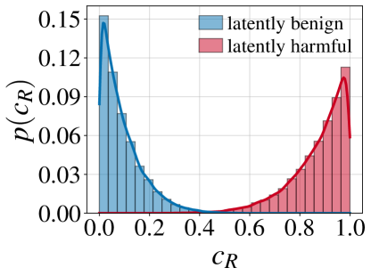
Since the viewports of popular electronic devices typically fit around five recommendations, as our synthetic data, we generate synthetic 5-out-regular graphs. We experiment with four graph sizes using three absorption probabilities, two shapes of probability distributions over out-edges, three fractions of latently harmful nodes, and two cost functions, one binary and one real-valued based on a mixture of two beta distributions as depicted in Fig. 12, to assign costs to nodes. We state the details on these parameters in Table 6. For each of the resulting $144$ configurations, we place edges using two different edge-placement models, SU and SH, for a total of $288$ graphs. For each node $i$, SU chooses $d$ distinct nodes $j\neq i$ as targets for its edges uniformly at random, whereas SH chooses $d$ distinct targets by sampling each $j$ with probability $\frac{1-|c(i)-c(j)|}{\sum_{j\in V}(1-|c(i)-c(j)|)}$. Hence, in SH, edges are drawn preferentially between nodes of similar costs, implementing homophily, whereas in SU, edges are drawn uniformly at random.

Figure 12. Histograms and kernel density estimates of $50\,000$ draws from the beta distributions used to assign costs to nodes in SU and SH under $c_{R}$. The cost of latently benign nodes is drawn from $\mathrm{Beta}(1,10)$, whereas the cost of latently harmful nodes is drawn from $\mathrm{Beta}(7,1)$.

(a) SU, cost function $c_{B}$

(b) SH, cost function $c_{B}$

(c) SU, cost function $c_{R}$

(d) SH, cost function $c_{R}$

Figure 13. Distributions of initial exposures $\mathbf{e}_{i}^{T}\mathbf{F}\mathbf{c}$ for nodes in SU and SH graphs with $100\,000$ nodes, for all combinations of absorption probabilities $\alpha\in\{0.05,0.1,0.2\}$ ($x$-axis label, first row), fractions of latently harmful nodes $\beta\in\{0.3,0.5,0.7\}$ ($x$-axis label, second row), and out-edge probability distributions $\chi\in\{\mathbf{U},\mathbf{S}\}$ (color). While the choice of the cost function barely makes a difference under random edge placements (SU, left), it has a tremendous impact under homophilous edge placements (SH, right).

E.1.2. Statistics

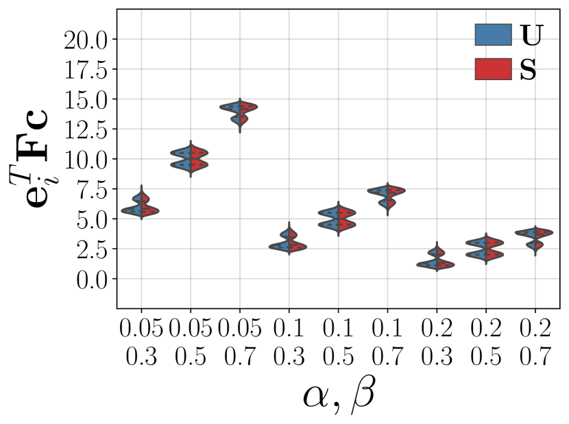
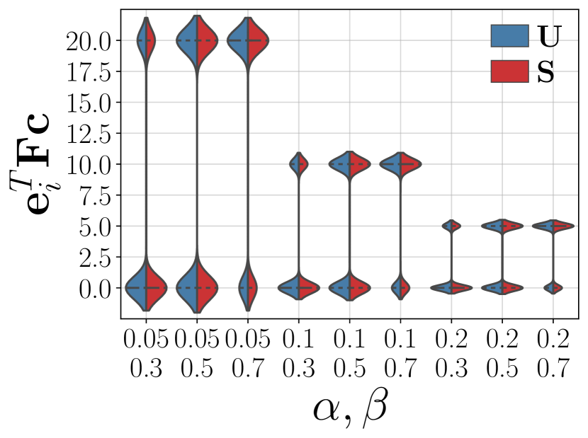
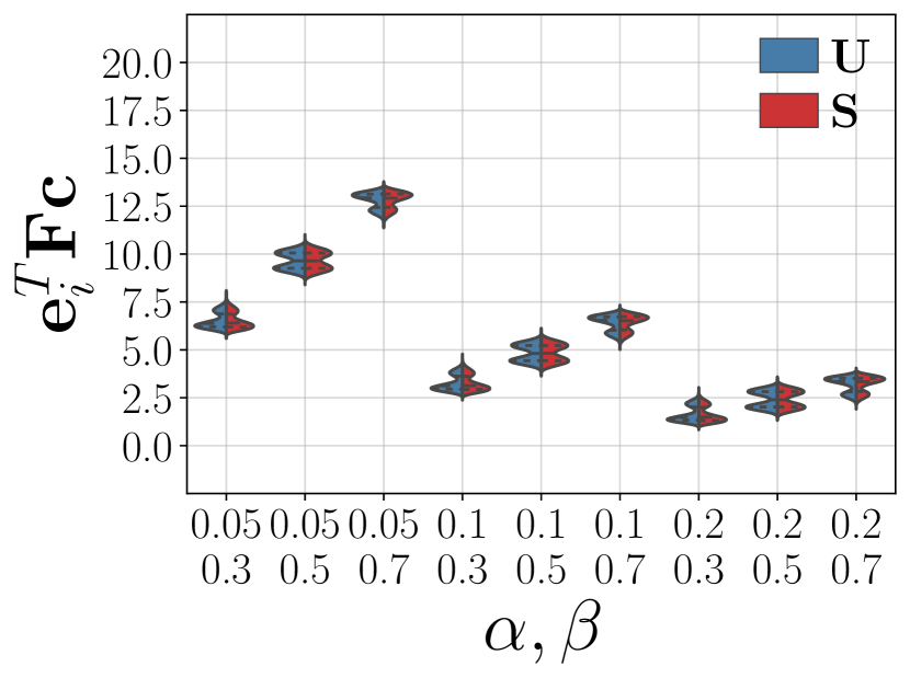
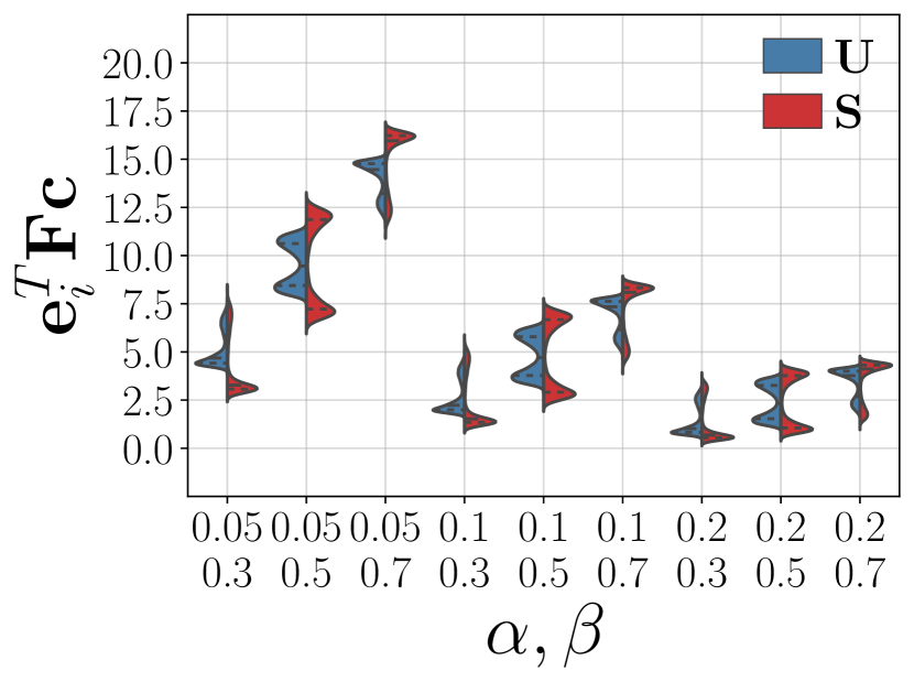
In Fig. 13, we show the distributions of initial exposures for nodes in our SU and SH graphs. For SU, we observe that the range of initial exposures is small and the cost function choice barely makes a difference, which is expected as edges are placed uniformly at random. In contrast, for SH, we observe the maximum range of initial exposures under $c_{B}$, as homophilous sampling under binary costs effectively splits the graph into two components consisting of harmful and benign nodes, respectively. Under $c_{R}$, we still observe a range of initial exposures that is twice to thrice as large as in SU graphs, and the probability shape $\chi\in\{\mathbf{U},\mathbf{S}\}$ strongly influences the distribution of initial exposures. These are again effects of homophilous sampling.

Table 6. Parameters used to generate SU and SH graphs.

Parameter	Meaning
$d=5$	Regular out-degree
$n\in\{10^{i}\mid i$ 1000$\in\{2,3,4,5\}\}$	Number of nodes in $G$
$\alpha\in\{0.05,0.1,0.2\}$	Random-walk absorption probability
$\chi\in\{\mathbf{U},\mathbf{S}\}$	Probability shape over a node’s out-edges: – Uniform – $\big{(}p_{ij}=\frac{1-\alpha}{d}$ for all $(i,j)\in E\big{)}$; – Skewed – $\big{(}\frac{1-\alpha}{d}\cdot p$ for $p\in\langle 0.35,0.25,0.20,0.15,0.05\rangle\big{)}$
$\beta\in\{0.3,0.5,0.7\}$	Fraction of latently harmful nodes – SU: fraction of nodes $i$ with $c_{i}=1$ – SH: fraction of nodes drawn from the beta – distribution with parameters $\alpha=7$, $\beta=1$
$c\in\{c_{B},c_{R}\}$	Cost functions – $c_{B}(i)=\begin{cases}1&\text{if $i$ is latently harmful}\\ 0&\text{otherwise}\\ \end{cases}$ – $c_{R}(i)=\begin{cases}\mathrm{Beta}(7,1)&\text{if $i$ is latently harmful}\\ \mathrm{Beta}(1,10)&\text{otherwise}\\ \end{cases}$

E.2. Real-World Data

E.2.1. Preprocessing

YouTube datasets

For our YouTube datasets, like Fabbri et al. (Fabbri et al., 2022), who experiment with a prior (not uniquely identified) version of this dataset, we generate $d$-regular recommendation graphs for $d\in\{5,10,20\}$ that contain only videos with at least 100 000, resp. 10 000, views as nodes (YT-100k, resp. YT-10k). Similar to Fabbri et al. (Fabbri et al., 2022) we treat the observed recommendations as implicit feedback interactions, eliminate sinks in the observed recommendation graph, use alternating least squares to generate relevance scores (Hu et al., 2008), and then take the nodes with the top scores as targets of out-edges in our reconstructed recommendation graphs. We additionally distinguish three absorption probabilities $\alpha\in\{0.05,0.1,0.2\}$ and two shapes $\chi\in\{\mathbf{U},\mathbf{S}\}$ of probability distributions over out-edges in our random-walk model, which leaves us with 36 transition matrices from six underlying graph structures.

NELA-GT datasets

To create our NELA-GT datasets, we restrict ourselves to news items of at least 140 characters (thus excluding boilerplate messages which we suspect were captured by accident) that were published in January 2021 by one of the 341 outlets for which all veracity labels are present, and consider the articles containing the authors’ January 6 keywords (NF-Jan06), the articles containing the authors’ COVID-19 keywords (NF-Cov19), and the collection containing all articles (NF-All). After embedding all news items using the all-MiniLM-L6-v2 model from the Sentence-Transformers library (Reimers and Gurevych, 2019), we compute pairwise cosine similarities $\cos(i,j)$ between all articles from the respective collection, transform these similarities into relevance scores between 0 and 1 via min-max-normalization ($\mathbf{R}[i,j]=\frac{\cos(i,j)+1}{2}$), and take the news items with the highest scores as targets of out-edges in our initial news feed graphs.

E.2.2. Cost functions

For both the YT and the NF datasets, we measure performance based on four different cost functions $c$ from two binary and two real-valued assignments of costs to channels and their videos ($c_{B1}$, $c_{B2}$, resp. $c_{R1}$, $c_{R2}$).

YouTube datasets

Our cost functions for the YT datasets map the channel categories provided with the original dataset to costs based on different mapping rules. Table 7 details the assignment of costs to video channels under our four different cost functions, and in Table 8, we provide the number of videos and the number of channels per category in YT-100k and YT-10k. Additionally, Table 9 lists the expected initial exposures of nodes in each of our YouTube recommendation graphs.

NELA-GT datasets

The costs we assign to nodes in our NF datasets are based on the Media Bias/Fact Check scores as well as the questionable source and conspiracy/pseudoscience flags of news outlets provided with the original dataset. As the number of news outlets covered by this dataset is too large to detail their individual cost assignments, here, we instead state how we transform the labels provided with the dataset into cost assignments under our four different cost functions. We define

$$c_{B1} =\begin{cases}1&\text{if}~{}\texttt{questionable\_source}=1\\ &\text{or}~{}\texttt{conspiracy\_pseudoscience}=1\\ 0&\text{otherwise,}\end{cases}$$

$$c_{B2} =\begin{cases}1&\text{if}~{}\texttt{factuality}\leq 2\\ 0&\text{otherwise,}\end{cases}$$

$$c_{R1} =1-\frac{\texttt{factuality}}{5}\;,~{}\text{and}$$

$$c_{R2} =1-\frac{\texttt{label}}{2}\;,$$

where typewritten variables are the names of the corresponding columns in the original data, $\texttt{questionable\_source}\in\{0,1\}$, $\texttt{conspiracy\_pseudoscience}\in\{0,1\}$, $\texttt{factuality}\in\{0,1,2,3,4,5\}$, and $\texttt{label}\in\{0,1,2\}$ is an aggregate label combining the other scores. An overview of the resulting cost assignments in each of our NF datasets is given in Table 10. In Table 11, we additionally state the expected total exposure as well as the total segregation and the maximum segregation from Fabbri et al. (Fabbri et al., 2022) for all NF datasets with $\alpha=0.05$ and $\chi=\textbf{U}$.

Table 7. Costs of videos from each channel under our four different cost functions.

Category	$c_{B1}$	$c_{B2}$	$c_{R1}$	$c_{R2}$
Alt-lite	1.0	1.0	0.8	0.8
Alt-right	1.0	1.0	1.0	1.0
Incel	0.0	1.0	0.4	0.6
IDW	1.0	1.0	0.6	0.2
MGTOW	0.0	1.0	0.4	0.6
MRA	0.0	1.0	0.2	0.4
NONE	0.0	0.0	0.0	0.0
PUA	0.0	1.0	0.2	0.4
center	0.0	0.0	0.0	0.0
left	0.0	0.0	0.0	0.0
left-center	0.0	0.0	0.0	0.0
right	0.0	0.0	0.0	0.0
right-center	0.0	0.0	0.0	0.0

E.2.3. Statistics

In-degree distributions

As our real-world graphs are $d$-out-regular by construction, their out-degree distributions are uniform. In contrast, the in-degree distributions of these graphs are highly skewed. In Fig. 14, we show the normalized in-degree distributions of our two largest real-world datasets, NF-All and YT-10k. Note that in-degrees, at least visually, appear to be exponentially distributed in the NF-All graph and power-law distributed in the YT-10k graph. Further, as illustrated in Fig. 15, even when considering only non-zero in-degrees and all real-world graphs, the NF graphs appear to be about an order of magnitude less skewed than the YT graphs.

Table 8. Number of videos $|V|$ and number of channels $|C|$ for each of our YouTube datasets.

	YT-100k	YT-10k	YT-100k	YT-10k
Category	$|V|$	$|V|$	$|C|$	$|C|$
Alt-lite	8 908	31 483	90	106
Alt-right	658	4 685	41	71
Incel	44	322	13	28
IDW	6 720	19 146	79	85
MGTOW	431	6 863	49	71
MRA	167	1 522	17	27
NONE	2 477	6 590	21	30
PUA	4 414	14 209	87	119
center	2 503	10 117	16	16
left	4 433	14 705	16	16
left-center	8 587	33 617	24	24
right	370	3 253	6	6
right-center	703	4 060	5	5

(a) NF-All

(b) YT-10k

Figure 14. Normalized in-degree distributions of our two largest real-world datasets for $d=20$. The in-degree distribution of the YT-10k graph is considerably more skewed than the in-degree distribution of the NF-All graph.

(a) NF

(b) YT

Figure 15. Distributions of nonzero in-degrees $\delta^{-}\!(i)$, normalized by the number of edges $m$, for each of our real-world datasets. The NF datasets are an order of magnitude more balanced than the YT datasets, and within one collection, smaller graphs have more skewed in-degree distributions.

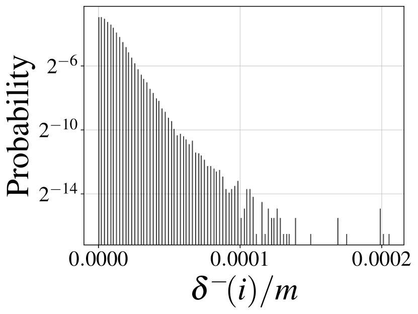
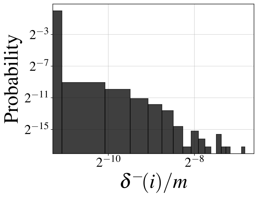
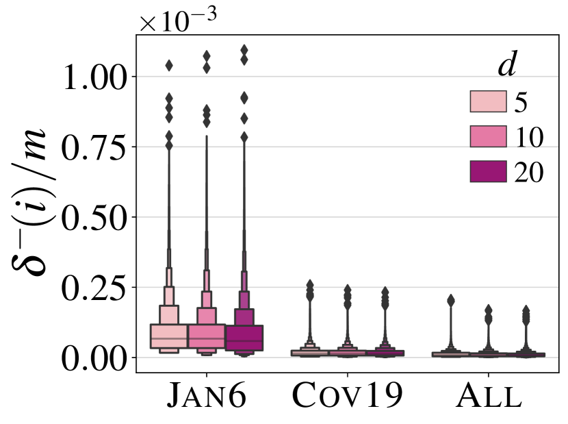
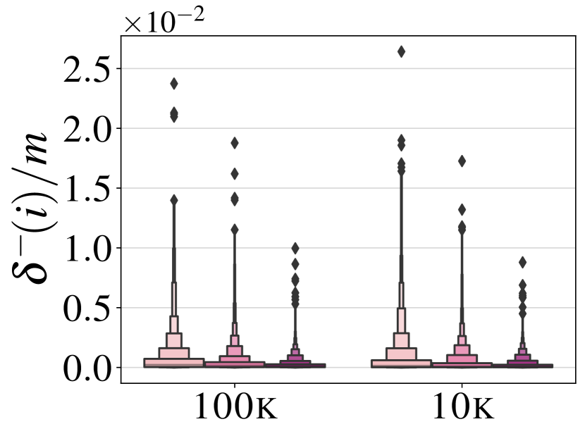
Relevance-score distributions

Complementing the discussion in the main paper, in Fig. 16, we show the relevance score distribution for each of our real-world datasets. Note that the nDCG used in our QREM experiments does not expect relevance scores to lie within a particular range, and that the relevance scores obtained by preprocessing YT are not strictly bounded, but they are guaranteed to mostly lie between $0$ and $1$, whereas the relevance scores obtained by preprocessing NF are directly cosine similarities, rescaled to lie between $0$ and $1$. As the relevance scores of the NF datasets are very concentrated, the quality threshold $q$ hardly constrains our rewiring options when solving QREM on NF graphs.

Table 9. Expected initial exposure $\nicefrac{{f(G)}}{{n}}$ of nodes in $G$ for the YouTube datasets.

	$d$	$\alpha$	$\chi$	$c_{B1}$	$c_{B2}$	$c_{R1}$	$c_{R2}$
YT-100k	5	0.05	S	6.318	8.129	4.335	2.518
			U	6.506	8.475	4.486	2.637
		0.10	S	3.251	4.245	2.303	1.491
			U	3.357	4.412	2.377	1.530
		0.20	S	1.694	2.234	1.245	0.900
			U	1.737	2.297	1.272	0.908
	10	0.05	S	6.387	8.316	4.440	2.688
			U	6.605	8.701	4.623	2.842
		0.10	S	3.355	4.417	2.395	1.584
			U	3.466	4.590	2.482	1.647
		0.20	S	1.750	2.317	1.290	0.938
			U	1.796	2.382	1.324	0.961
	20	0.05	S	6.983	9.026	4.880	3.014
			U	7.372	9.444	5.153	3.195
		0.10	S	3.606	4.716	2.582	1.722
			U	3.749	4.874	2.687	1.801
		0.20	S	1.844	2.429	1.359	0.989
			U	1.894	2.486	1.398	1.022
YT-10k	5	0.05	S	4.198	5.597	2.992	1.926
			U	4.173	5.785	3.040	2.066
		0.10	S	2.330	3.217	1.734	1.244
			U	2.401	3.369	1.801	1.315
		0.20	S	1.309	1.854	1.019	0.806
			U	1.353	1.922	1.053	0.834
	10	0.05	S	5.093	6.729	3.641	2.377
			U	5.712	7.576	4.101	2.704
		0.10	S	2.729	3.743	2.027	1.448
			U	2.958	4.063	2.203	1.584
		0.20	S	1.450	2.046	1.125	0.883
			U	1.525	2.152	1.185	0.932
	20	0.05	S	6.185	8.186	4.405	2.820
			U	6.741	8.987	4.819	3.094
		0.10	S	3.120	4.285	2.310	1.625
			U	3.306	4.569	2.460	1.741
		0.20	S	1.577	2.228	1.222	0.949
			U	1.638	2.324	1.275	0.996

Presence of safe nodes

In 3 and 1, we established that if a graph $G$ has at least $\Lambda^{+}$ safe nodes, where a node $i$ is safe if its exposure $\mathbf{e}_{i}^{T}\mathbf{F}\mathbf{c}$ is $0$ and $\Lambda^{+}$ is the maximum degree of an unsafe node in $G$, then we can approximate $f_{\Delta}$ up to a factor of $(1-\nicefrac{{1}}{{e}})$. In Fig. 17, we demonstrate that under all our cost functions, this applies to all YT graphs and roughly two thirds of the NF graphs, with the notable exception of news articles on the topic of January 6 (i.e., content reporting on the Capitol riot). Hence, our theoretical approximation guarantee mostly holds also in practice.

Table 10. Number of news outlets $|C|$ and number of videos $|V|$ in each of our NELA-GT-2021 datasets, for each unique combination of assigned costs.

					NF-Jan6	NF-Cov19	NF-All
$c_{B1}$	$c_{B2}$	$c_{R1}$	$c_{R2}$	$|C|$	$|V|$	$|V|$	$|V|$
0	0	0.0	0.0	4	147	631	993
0	0	0.2	0.0	69	3188	17794	29021
0	0	0.4	0.0	18	1463	3986	6549
0	1	0.6	0.0	1	0	0	0
0	1	0.6	1.0	40	3920	19398	32303
1	1	0.6	0.5	73	1533	8804	15549
1	1	0.8	0.5	112	1497	6436	14337
1	1	1.0	0.5	24	237	983	1987

Table 11. Initial expected total exposure to harm $f(G)$, as well as total segregation and maximum segregation from Fabbri et al. (Fabbri et al., 2022), on each of our NF graphs with $\alpha=0.05$, $\chi=\textbf{U}$, and $\mu=1.0$ for segregation computations under $c_{R1}$ and $c_{R2}$.

	$d$	$c$	$f(G)$	Total Seg.	Max. Seg.
NF-Jan06	5	$c_{B1}$	51 940	6 896	19.99
		$c_{B2}$	118 506	25 038	19.99
		$c_{R1}$	104 948	259	2.04
		$c_{R2}$	92 536	8 555	19.99
	10	$c_{B1}$	50 682	5 342	5.79
		$c_{B2}$	114 141	18 151	19.99
		$c_{R1}$	103 482	250	1.47
		$c_{R2}$	88 800	6 172	10.33
	20	$c_{B1}$	50 319	4 889	4.05
		$c_{B2}$	113 738	16 194	6.50
		$c_{R1}$	103 445	246	1.21
		$c_{R2}$	88 579	5 782	2.93
NF-Cov19	5	$c_{B1}$	264 781	54 699	19.99
		$c_{B2}$	635 867	201 579	19.99
		$c_{R1}$	520 763	1 075	2.19
		$c_{R2}$	503 477	81 903	19.99
	10	$c_{B1}$	252 294	44 313	19.99
		$c_{B2}$	618 645	157 105	19.99
		$c_{R1}$	513 982	1 038	1.86
		$c_{R2}$	492 498	65 199	19.99
	20	$c_{B1}$	248 708	38 597	19.99
		$c_{B2}$	617 014	134 998	19.99
		$c_{R1}$	513 113	1 020	1.48
		$c_{R2}$	492 660	56 696	19.05
NF-All	5	$c_{B1}$	520 092	128 388	19.99
		$c_{B2}$	1 111 742	383 640	19.99
		$c_{R1}$	890 383	3 013	19.99
		$c_{R2}$	851 697	136 356	19.99
	10	$c_{B1}$	496 667	103 825	19.99
		$c_{B2}$	1 089 690	307 444	19.99
		$c_{R1}$	880 536	2 666	15.10
		$c_{R2}$	841 357	111 298	19.99
	20	$c_{B1}$	480 186	88 983	19.99
		$c_{B2}$	1 076 287	260 998	19.99
		$c_{R1}$	874 785	2 187	6.90
		$c_{R2}$	836 194	96 895	19.99

Figure 16. Distributions of relevance scores $\mathbf{R}[i,j]$ for each source node $i\in V$ and the top $100$ nodes $j$ considered as potential rewiring targets, for each of our real-world datasets in the QREM setting. The relevance distributions are much more skewed in the YT datasets than in the NF datasets.

(a) NF

(b) YT

Figure 17. Fraction (color) and number (annotation) of safe nodes in each of our real-world graphs with degrees $d\in\{5,10,20\}$, under our four cost functions $c\in\{c_{B1},c_{B2},c_{R1},c_{R2}\}$. In all YT graphs and roughly two thirds of the NF graphs, the precondition of 3 holds, such that the greedy algorithm can approximate $f_{\Delta}$ up to a factor of $(1-\frac{1}{e})$.

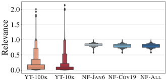
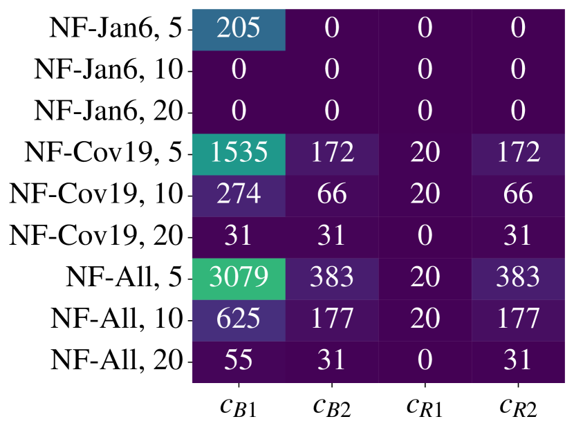
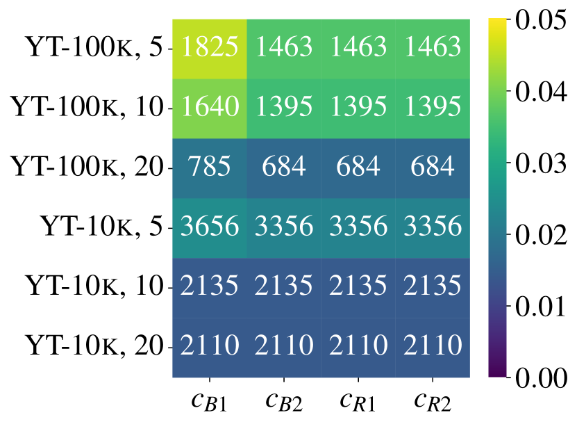
Impact of cost-function noise

To see how errors in harmfulness assessment might impact our ability to rewire edges effectively, we investigate the behavior of our exposure objective under noise in the cost function. In particular, we assess how the distribution of node exposures shifts when we change the original cost vector $\mathbf{c}$ to a cost vector $\mathbf{c}^{\prime}$ by either swapping the cost of a randomly chosen harmful node with that of a randomly chosen benign node (cost swaps), or setting the cost $c_{i}$ of a randomly chosen node $i$ to its opposite, i.e., $1-c_{i}$ (cost flips). Illustrating the results on the YT-100k dataset in Fig. 18, we observe that as expected—and by construction—, node exposures are generally sensitive to individual cost assignments. However, the median impact of moderate cost-function noise on node exposure levels is close to zero, and the most extreme cost fluctuations occur for nodes whose observed exposure decreases as compared to their actual exposure. The latter might lead Gamine to undervalue some highly exposed nodes in its rewiring considerations, but this risk is unavoidable when dealing with noisy data. In contrast to prior work, Gamine uses an exposure objective that depends on the cost assignments of all nodes in the graph. Overall, our experiments with node-level cost-function noise demonstrate that this objective decays rather smoothly—not only in theory but also in practice.

(a) Cost flips

(b) Cost swaps

Figure 18. Distribution of differences between node exposures before and after the introduction of noise, shown for the YT-100k dataset with $d=5$, $\alpha=0.05$, and $\chi\in\{\mathbf{U},\mathbf{S}\}$, as measured under $c_{R1}$. Negative values signal that adding noise decreased the exposure to harm of a particular node.

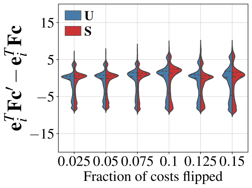
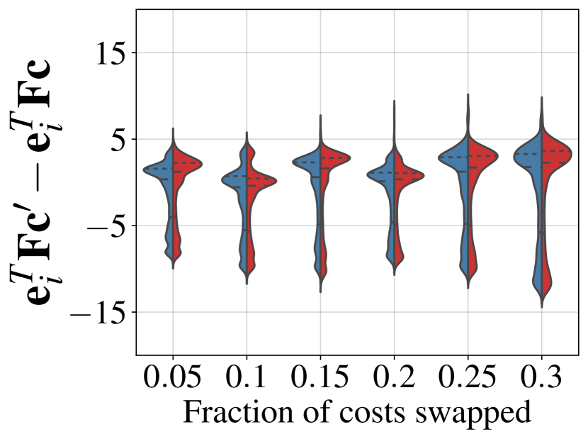
Appendix F Further Experiments

F.1. Impact of Modeling Choices

In the main text, we only demonstrated the impact of the quality threshold $q$ on the performance of Gamine. Here, we further discuss the performance impact of the regular out-degree $d$, the absorption probability $\alpha$, the shape of the probability distribution over out-edges $\chi$, and the cost function $c$.

Impact of regular out-degree $d$

Since the impact of individual edges on the objective function decreases as $d$ increases, for a given budget $r$, we expect Gamine to reduce our objective more strongly for smaller values of $d$. This is exactly what we find, as illustrated in Fig. 19, and the pattern persists across absorption probabilities $\alpha$, probability shapes $\chi$, quality thresholds $q$, and cost functions $c$.

Impact of absorption probability $\alpha$ and out-edge probability distribution shape $\chi$

For smaller random-walk absorption probabilities $\alpha$, we obtain longer random walks and thus higher exposure to harmful content, and for $\chi=\mathbf{S}$, some edges are traversed particularly often. Thus, given a constant budget $r$, we expect Gamine to achieve a larger decrease of $f$ for smaller $\alpha$, and an initially faster decrease on graphs with skewed out-edge probability distributions. Again, this is what we find, as depicted in Fig. 20.

Impact of cost function $c$

As the binary cost function $c_{B1}$ (used also in (Fabbri et al., 2022) on a prior version of the data from (Ribeiro et al., 2020)) labels only videos from Alt-Right, Alt-Lite, and Intellectual Dark Web (IDW) channels as harmful ($c_{B1}=1$) and all other videos as benign ($c_{B1}=0$), whereas all other cost functions also assign positive cost to videos from anti-feminist channels (Incel, MGTOW, MRA, and PUA) (cf. Table 7), we expect Gamine to perform strongest under $c_{B1}$. As exemplified in Fig. 21, this is exactly what we observe, and the pattern persists across regular out-degrees $d$, absorption probabilities $\alpha$, distribution shapes $\chi$, and quality thresholds $q$. Interestingly, we also consistently observe that Gamine is roughly equally strong under the binary cost function $c_{B2}$ and the real-valued cost function $c_{R1}$, and weakest under the real-valued cost function $c_{R2}$. As $c_{R1}$ and $c_{R2}$ differ only in how they assign costs to videos from IDW and anti-feminist channels, with $c_{R1}$ ($c_{R2}$) placing IDW to the right (left) of anti-feminist channels, this means that reducing the exposure to harm is harder when we consider the IDW more benign than anti-feminist communities, even though there are more IDW videos in YT-100k than videos from all anti-feminist communities combined.

(a) Absorption probability $\alpha=0.05$

(b) Absorption probability $\alpha=0.1$

Figure 19. Performance of Gamine for out-regular degrees $d\in\{5,10,20\}$, run with $q=0.0$ under $c_{B1}$ on YT-100k with $\chi=\mathbf{U}$. The smaller the out-degree, the stronger Gamine.

(a) Cost function $c_{R1}$

(b) Cost function $c_{B1}$

Figure 20. Performance of Gamine for absorption probabilities $\alpha\in\{0.05,0.1,0.2\}$ and out-edge probability distribution shapes $\chi\in\{\mathbf{U},\mathbf{S}\}$, run with $q=0.5$ on YT-100k with $d=5$. The smaller the absorption probability, the stronger the performance of Gamine, and our objective function drops faster when the out-edge probability distribution is skewed.

(a) Quality threshold $q=0.99$

(b) Quality threshold $q=0.0$

Figure 21. Performance of Gamine under cost functions $c\in\{c_{B1},c_{B2},c_{R1},c_{R2}\}$, run on YT-100k with $d=5$, $\alpha=0.05$, and $\chi=\mathbf{U}$. Gamine is strongest under the binary cost function $c_{B1}$, weakest under the real-valued cost function $c_{R2}$, and roughly equally strong under the binary $c_{B2}$ and the real-valued $c_{R1}$.

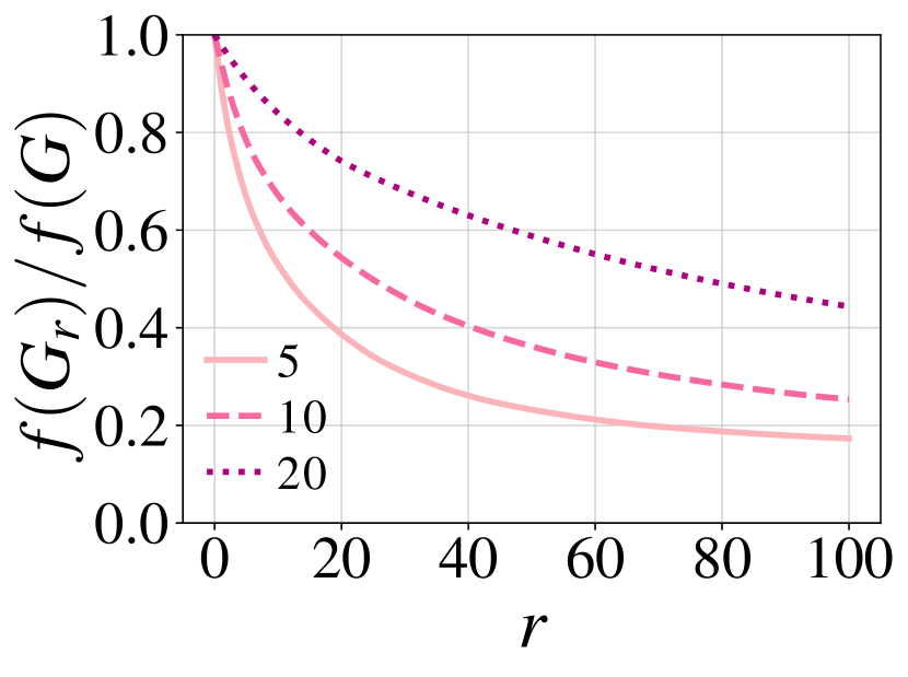
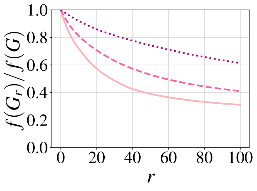
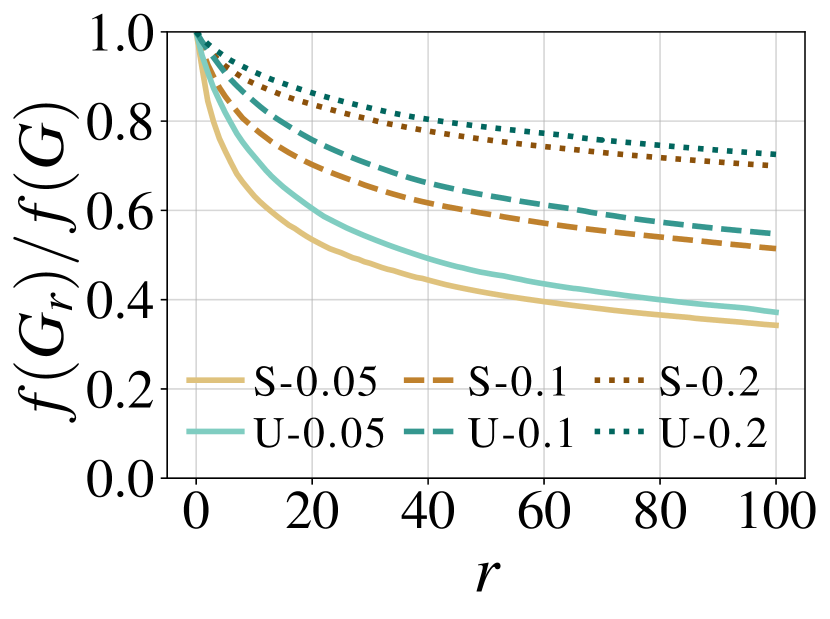
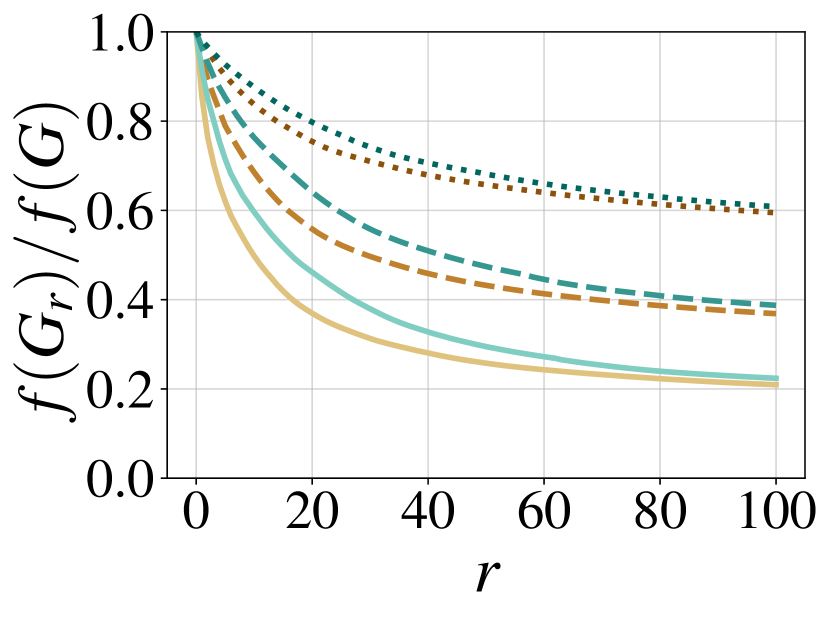
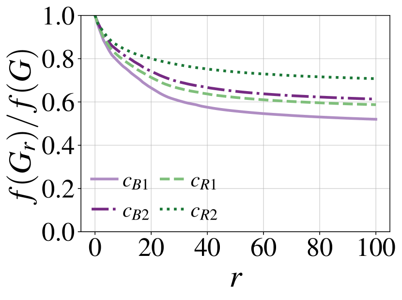
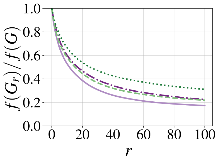
F.2. Scalability

F.2.1. Precomputations

In Fig. 5 in the main text, we showed that Gamine’s individual edge rewirings scale approximately linearly in practice, whereas MMS’s individual edge rewirings scale quadratically. In Fig. 22, we additionally show that precomputations add approximately linear overhead for Gamine and somewhat unpredictable, at times quadratic overhead for MMS. This could be due to two factors. First, the relevance precomputations for MMS are slightly more complicated than for Gamine. Second, one part of MMS’s precomputations not present in Gamine is a matrix inverse approximation via power iteration. This computation is quadratic in the number of harmful nodes, as MMS considers only these nodes as transient states.

(a) Gamine on REM

(b) Gamine and MMS on QREM

Figure 22. Empirical scaling of precomputations for Gamine and MMS, computed with $\alpha=0.05$, $\chi=\mathbf{U}$, $c_{B1}$, and $q=0.0$ (REM) resp. $0.99$ (QREM). We depict scaling for REM as a function of $n$, with a linear regression fitted across datasets, and scaling for QREM as a function of $m$, where we connect the observations stemming from different regular out-degrees of the same dataset for NF-Cov19, NF-All, and YT-10k. Precomputations for REM are much faster than for QREM, and while Gamine scales approximately linearly, MMS scales somewhat unpredictably.

Figure 23. Empirical scaling of Gamine as a function of the quality threshold $q$, run on YT-100k with $\alpha=0.05$, $\chi=\mathbf{U}$, and $c_{B1}$, for $d\in\{5,10,20\}$. The larger $q$, the faster Gamine.

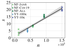
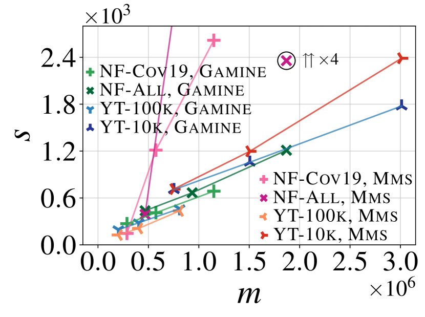
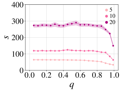
F.2.2. Impact of quality threshold

In addition to Gamine’s scaling behavior as a function of $n$ and $m$, for QREM, we would like to understand how the scaling behavior of our method depends on the quality threshold $q$. To this end, we run Gamine on each of our YT-100k datasets with $q\in\{\nicefrac{{x}}{{100}}\mid 0<x<100,x\mod 5=0\}\cup\{0.99\}$. Since increasing $q$ eliminates rewiring candidates, we hope to see the running time decrease as $q$ increases, and we expect a larger acceleration on graphs with higher (regular) out-degrees. As reported in Fig. 23, this is precisely what we find—and the dependence on $q$ is particularly small for our sparser YT-100k datasets.

(a) SH, $n=100$

(b) SU, $n=100$

(c) SU, $n=1\,000$

Figure 24. Correlation of the $\hat{\Delta}$ and $\Delta$ values for the $100$ candidates $(i,j,k)$ with the largest $\Delta$, in $10$ rewiring rounds on synthetic graphs with $\alpha=0.05$, $\beta=0.7$, and $\chi=\textbf{U}$, under our binary costs $c_{B}$. $\Delta$ and $\hat{\Delta}$ are almost perfectly correlated.

(a) Pearson’s Correlation

(b) Spearman’s Correlation

Figure 25. Pearsons’ product-moment correlation and Spearman’s rank correlation between $\Delta$ and $\hat{\Delta}$, in $10$ rewiring rounds on synthetic graphs with $\alpha=0.05$, $\beta=0.7$, and $\chi=\textbf{U}$, under binary costs. Both correlations are almost perfect across all rounds, and they are even closer to $1$ for the larger synthetic graphs than for the smaller ones.

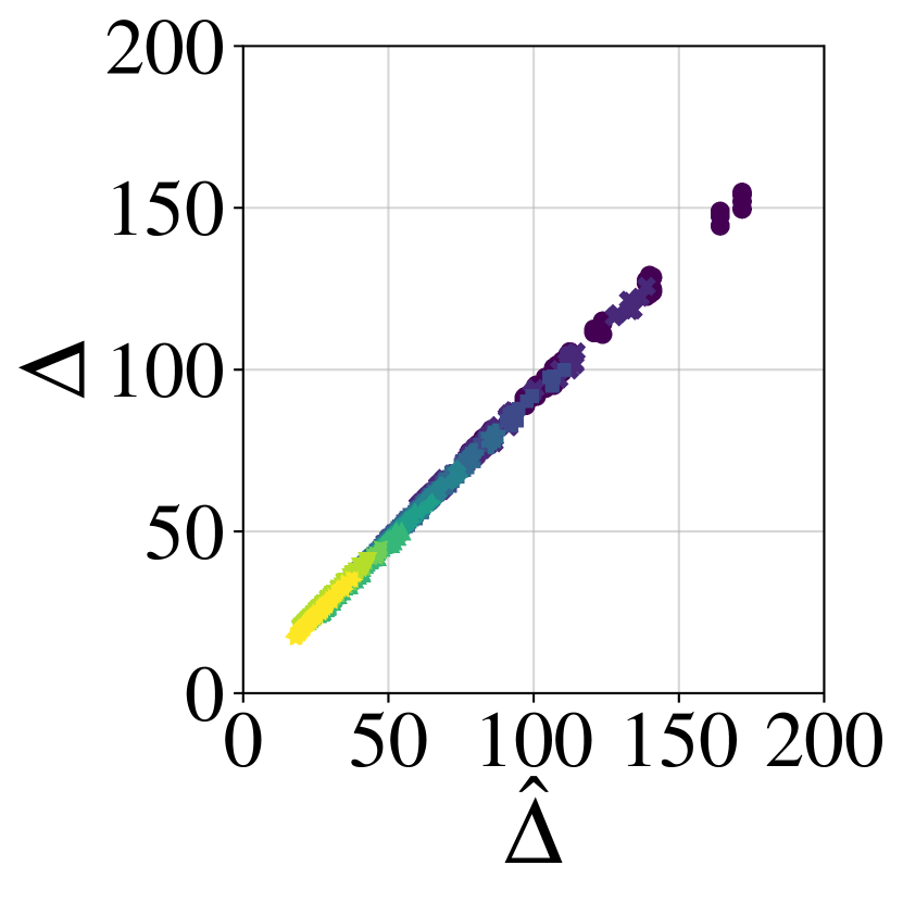
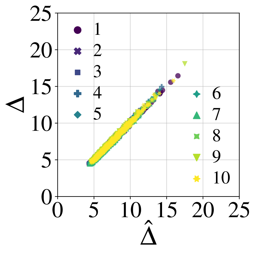
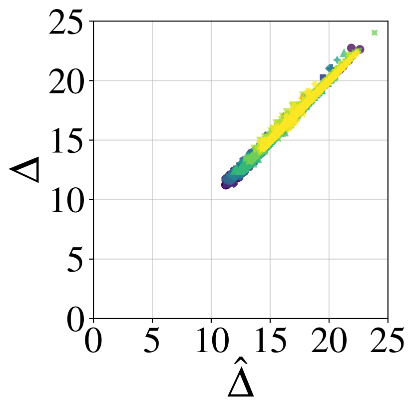
F.3. Impact of Using $\hat{\Delta}$ Instead of $\Delta$

Having confirmed in the main text that Gamine scales linearly not only in theory but also in practice (cf. Fig. 5), we would like to ensure that moving from $\Delta$ to $\hat{\Delta}$, which enables this scalability, has little impact on the quality of our results. To this end, we investigate the relationship between $\Delta$ and $\hat{\Delta}$ on the smallest instances of our synthetic graphs, SU and SH. As illustrated in Fig. 24, $\Delta$ and $\hat{\Delta}$ are almost perfectly correlated, and Fig. 25 shows that this holds not only for the top-ranked candidates but for all candidates, under both product-moment correlation and, more importantly, rank correlation. Thus, we are confident that our reliance on $\hat{\Delta}$, rather than $\Delta$, to select greedy rewirings hardly degrades our results.

F.4. Performance on the NELA-GT Datasets

Whereas on the YT datasets, $100$ rewirings with Gamine reduce the expected total exposure to harm by $50\%$ while guaranteeing recommendations still $95\%$ as relevant as the original recommendations (Fig. 2), the reduction we achieve on the NF datasets is more moderate. As illustrated in Fig. 26, our best result here is a reduction of the expected total exposure to harm by about $30\%$, again under a $95\%$ quality guarantee. Notably, changing the quality threshold $q$ has a smaller impact on the NF than on the YT datasets, and sometimes it has no performance impact at all. In fact, for the NF-Jan06 graphs involved in Fig. 26, $q=0.95\equiv 0.9\equiv 0.5$ (and hence, we only draw the line for $q=0.95$). This indicates that unlike on the YT datasets, on the NF datasets, Gamine is actually affected by the restriction of rewirings to the $100$ most relevant candidates, which we implement for all real-world datasets (cf. Section 6.1.2 and also Section E.2, Fig. 16).

(a) Cost function $c_{R2}$

(b) Cost function $c_{B1}$

Figure 26. Performance of Gamine on our NF datasets with $d=5$, $\alpha=0.05$, and $\chi=\textbf{U}$. Varying $q$ on the NF-Jan06 dataset has a much smaller performance impact than what we observed on the YT-100k dataset, and the relative reduction in the expected total exposure after $100$ rewirings is at the level of what we achieve after $10$ rewirings on the YT-100k dataset (cf. Fig. 2).

(a) Quality threshold $q=0.99$

(b) Quality threshold $q=0.5$

Figure 27. Performance of Gamine and MMS when measured under $c_{B1}$ by the maximum segregation or the total segregation from Fabbri et al. (Fabbri et al., 2022), or by the total exposure as defined in Eq. 3, run on NF-Jan06 with $d=5$, $\alpha=0.05$, and $\chi=\mathbf{U}$. Gamine outperforms MMS on the exposure objective, but MMS reduces its segregation objective more strongly. Counterintuitively, MMS achieves a stronger reduction of its segregation objective under a stricter quality threshold.

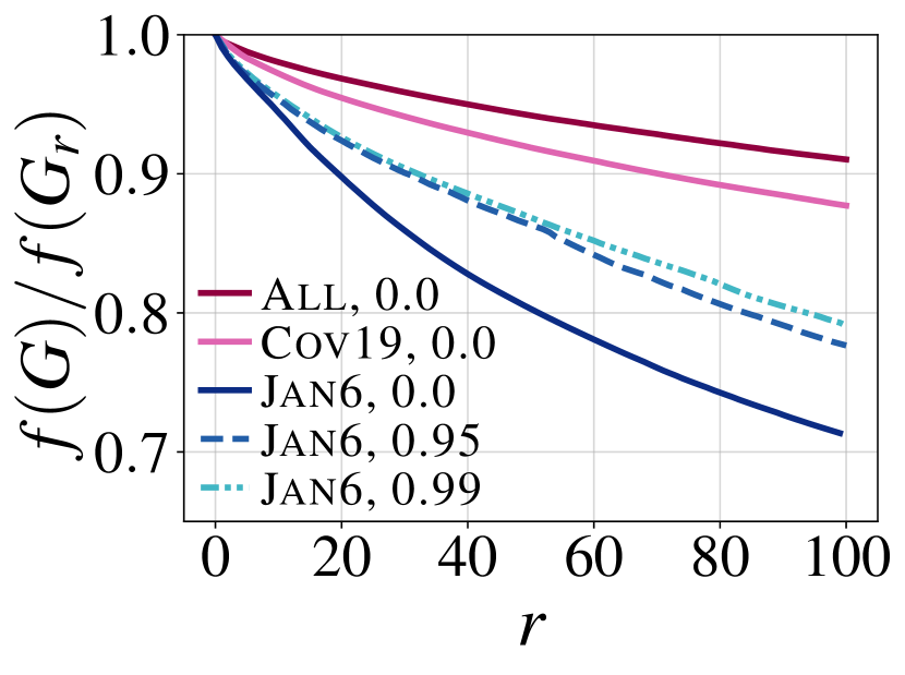
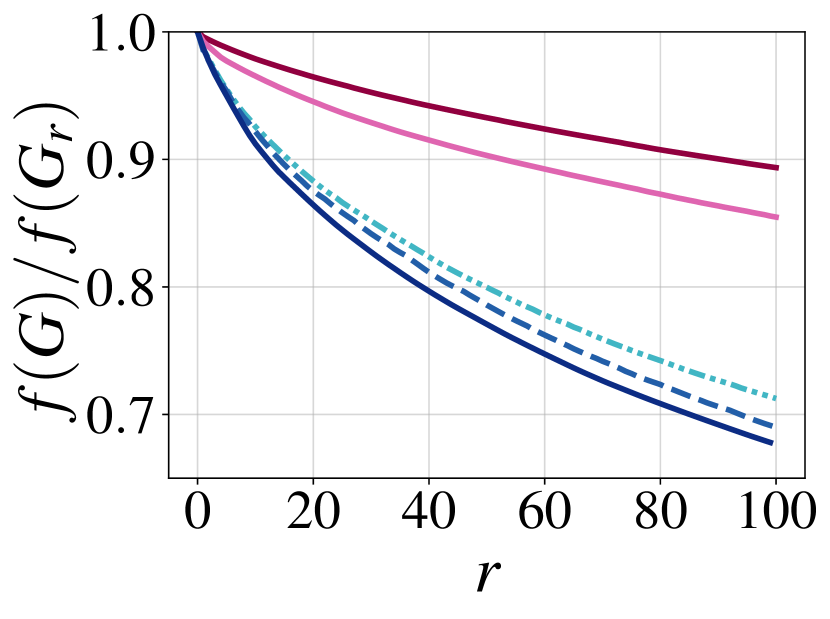
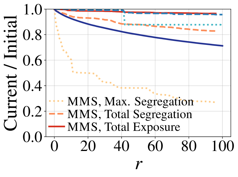
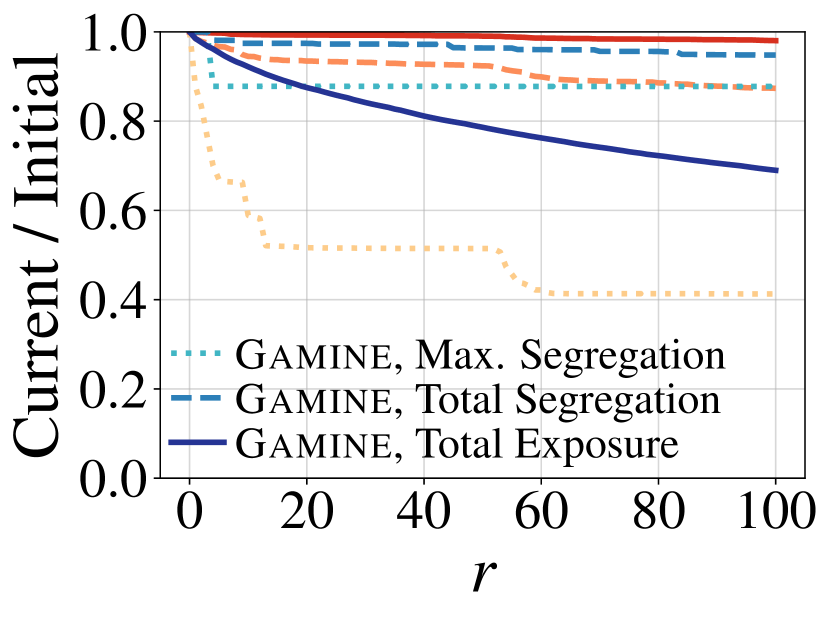
As illustrated in Fig. 27, on the NF-Jan06 dataset under $c_{B1}$, Gamine still outperforms MMS on our exposure objective, but MMS achieves a much stronger relative reduction of its segregation objective. However, MMS counterintuitively reduces its objective function more strongly under a stricter quality threshold—a behavior we never observe with Gamine under our exposure objective. As given the same recommendation sequence $\mathbf{r}_{i}$ at node $i$, a rewiring $(i,j,k)$ that is $q$-permissible under $q=0.99$ is also $q$-permissible under $q=0.5$, this suggests that MMS is highly dependent on its trajectory and sometimes requires greedily suboptimal choices to obtain the best possible result after $r$ rewirings.

Moreover, the promising performance we observe for MMS on NF-Jan06 under $c_{B1}$ does not carry over to NF-Cov19 and NF-All, or even to other cost functions on NF-Jan06: On NF-Cov19 and NF-All under $c_{B1}$, and on NF-Jan06 under $c_{B2}$ or $c_{R2}$ with binarization threshold $\mu=1.0$, MMS cannot reduce its segregation objective at all, even though the starting value of the maximum segregation is exactly the same as for NF-Jan06 under $c_{B1}$ (cf. Section E.2, Table 11). On NF-Jan06 under $c_{R2}$ with binarization threshold $\mu=1.0$, MMS stops after four rewirings with a reduction of $25\%$, but the maximum segregation is already miniscule from the start. Thus, our experiments on NF data confirm our impression from the main paper that MMS less robust than Gamine.

F.5. Edge Statistics of Rewired Edges

In the main text, we reported that Gamine frequently rewires edges $(i,j)$ with a comparatively large sum of in-degrees. To corroborate this claim, in Fig. 28, we compare the distribution of normalized in-degree sums for edges rewired by Gamine to that of all edges. We find that the distribution of in-degree sums for edges rewired by Gamine has a higher median than the distribution of in-degree sums for all edges, and that the former is generally shifted toward higher in-degree sums as compared to the latter.

(a) NF, $q=0.0$

(b) YT, $q=0.5$

Figure 28. Distributions of normalized in-degree sums $\frac{\delta^{-}\!(i)+\delta^{-}\!(j)}{m}$ for edges rewired by Gamine under $c_{B1}$ vs. all edges, on real-world graphs with $d=5$, $\alpha=0.05$, and $\chi=\mathbf{U}$. Gamine tends to rewire edges with larger in-degree sums.