A Theory of Unsupervised Speech Recognition

Liming Wang1, Mark Hasegawa-Johnson1    Chang D. Yoo2
1University of Illinois Urbana-Champaign
2Korea Advanced Institute of Science Technology
{lwang114,jhasegaw}@illinois.edu, cd_yoo@kaist.ac.kr
Abstract

Unsupervised speech recognition (ASR-U) is the problem of learning automatic speech recognition (ASR) systems from unpaired speech-only and text-only corpora. While various algorithms exist to solve this problem, a theoretical framework is missing to study their properties and addressing such issues as sensitivity to hyperparameters and training instability. In this paper, we proposed a general theoretical framework to study the properties of ASR-U systems based on random matrix theory and the theory of neural tangent kernels. Such a framework allows us to prove various learnability conditions and sample complexity bounds of ASR-U. Extensive ASR-U experiments on synthetic languages with three classes of transition graphs provide strong empirical evidence for our theory (code available at cactuswiththoughts/UnsupASRTheory.git).

1 Introduction

Unsupervised speech recognition (ASR-U) addresses the problem of learning automatic speech recognition (ASR) systems using unpaired speech-only and text-only corpora. Such a system not only significantly reduces the dependency on annotation resources required for training state-of-the-art ASR system, but it also serves as a bridge between spoken and written language understanding tasks in the low-resource settings. Since its first proposal Liu et al. (2018), it has seen remarkable progress, and the current best system Baevski et al. (2021) has achieved comparable performance to systems trained with paired data on various languages. However, there are several ambiguities surrounding ASR-U, which could impede future evolution of these systems. In particular, prior experiments have found that training the current state-of-the-art ASR-U model, wav2vec-U Baevski et al. (2021), requires careful tuning over the weights of various regularization losses to avoid converging to bad local optima and that even despite extensive regularization weight tuning, wav2vec-U may still fail to converge Ni et al. (2022). Therefore, it is ambiguous whether or when unpaired speech and text data indeed provide sufficient information for learning an ASR system. Another ambiguity is whether the success of existing ASR-U models based on generative adversarial net (GAN) Goodfellow et al. (2014) is sufficiently explained by the GAN objective function or requires other factors, such as randomness in training, quirks in the data used and careful domain-specific hyper-parameter settings.

This paper provides a theoretical analysis of ASR-U to clarify the ambiguity surrounding ASR-U. First, we prove learnability conditions and sample complexity bounds that depend on the eigenvalue spacings of the transition probability matrix of the spoken language. Random matrix theory shows that such learnability conditions are achievable with high probability. Next, we study the gradient flow of GAN-based ASR-U and provide conditions under which the generator minimizing the GAN objective converges to the true generator. Finally, to verify our theory empirically, we perform GAN-based ASR-U experiments on three classes of synthetic languages. Not only do we observe phase transition phenomena predicted by our theory, but we achieve stable training with a lower test word error rate by several modifications of the existing state-of-the-art ASR-U system inspired by our theory.

2 Problem formulation
Refer to caption
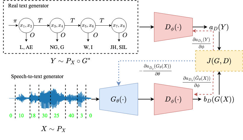
Figure 1: Overview of the ASR-U system for our analysis

General formulation

The training data consists of quantized speech sequences and phoneme label sequences. The two sequences are unpaired: no label sequence matches any one of the speech sequences. The data are, however, matched in distribution. Let PXi(x)subscript𝑃subscript𝑋𝑖𝑥P_{X_{i}}(x) and PYj(y)subscript𝑃subscript𝑌𝑗𝑦P_{Y_{j}}(y) be the probability mass functions (pmfs) of the ithsuperscript𝑖thi^{\textrm{th}} speech vector in a sequence, x𝕏𝑥𝕏x\in{\mathbb{X}}, and the jthsuperscript𝑗thj^{\textrm{th}} phoneme in a sequence, y𝕐𝑦𝕐y\in{\mathbb{Y}}, respectively: the requirement that they are matched in distribution is the requirement that there exists some generator function O:(𝕏,𝕐){0,1}:𝑂𝕏𝕐01O:({\mathbb{X}},{\mathbb{Y}})\rightarrow\{0,1\} such that

x𝕏PXi(x)O(x,y)=PYi(y)subscript𝑥𝕏subscript𝑃subscript𝑋𝑖𝑥𝑂𝑥𝑦subscript𝑃subscript𝑌𝑖𝑦\displaystyle\sum_{x\in{\mathbb{X}}}P_{X_{i}}(x)O(x,y)=P_{Y_{i}}(y) (1)

The problem of ASR-U is to find the generator function O𝑂O.

GAN-based ASR-U

Eq. (1) leverages sequence information to remove ambiguity: O𝑂O must be an optimal generator not only for the position-independent distributions of X𝑋X and Y𝑌Y, but also for their position-dependent distributions PXi,PYii0subscript𝑃subscript𝑋𝑖subscript𝑃subscript𝑌𝑖for-all𝑖superscript0P_{X_{i}},P_{Y_{i}}\forall i\in{\mathbb{N}}^{0}. In reality we cannot observe every possible sequence of speech vectors, or every possible sequence of phonemes, but instead must estimate O𝑂O from samples. To address this issue, a GAN can be used to reproduce the empirical distribution of the training dataset with minimum error, subject to the generator’s inductive bias, e.g., subject to the constraint that the function O𝑂O is a matrix of the form O{0,1}|𝕏|×|𝕐|𝑂superscript01𝕏𝕐O\in\{0,1\}^{|{\mathbb{X}}|\times|{\mathbb{Y}}|}, where |𝕏|𝕏|{\mathbb{X}}| and |𝕐|𝕐|{\mathbb{Y}}| are the sizes of the alphabets 𝕏𝕏{\mathbb{X}} and 𝕐𝕐{\mathbb{Y}}, respectively. As shown in Figure 1, a GAN achieves this goal by computing O𝑂O as the output of a neural network, O=G(x,y;θ)𝑂𝐺𝑥𝑦𝜃O=G(x,y;\theta), and by requiring G𝐺G to play a zero-sum game with another neural network called the discriminator D𝐷D with the following general utility function:

minGmaxDJ(G,D):=𝔼YPY[a(D(Y))]𝔼XPX[b(D(G(X)))].assignsubscript𝐺subscript𝐷𝐽𝐺𝐷subscript𝔼similar-to𝑌subscript𝑃𝑌delimited-[]𝑎𝐷𝑌subscript𝔼similar-to𝑋subscript𝑃𝑋delimited-[]𝑏𝐷𝐺𝑋\min_{G}\max_{D}J(G,D):=\mathbb{E}_{Y\sim P_{Y}}[a(D(Y))]-\\ \mathbb{E}_{X\sim P_{X}}[b(D(G(X)))]. (2)

For the original GAN Goodfellow et al. (2014), a(D)=log(σ(D))𝑎𝐷𝜎𝐷a(D)=\log(\sigma(D)) and b(D)=log(1σ(D))𝑏𝐷1𝜎𝐷b(D)=-\log(1-\sigma(D)), where σ𝜎\sigma is the sigmoid function. For the Wasserstein GAN Arjovsky et al. (2017), D(Y)𝐷𝑌D(Y) is a Lipschitz-continuous scalar function, and a(D)=b(D)=D𝑎𝐷𝑏𝐷𝐷a(D)=b(D)=D. A maximum mean discrepancy (MMD) GAN Li et al. (2017) minimizes the squred norm of Eq. (2), where D(Y)𝐷𝑌D(Y) is an embedding into a reproducing kernel Hilbert space (RKHS). In this paper we take the RKHS embedding to be the probability mass function of a scalar random variable D(Y)𝐷𝑌D(Y), and assume that the discriminator is trained well enough to maintain Eq. (2). In this situation, the MMD GAN minimizes Eq. (2) with a(D)=b(D)=Y𝑎𝐷𝑏𝐷𝑌a(D)=b(D)=Y. In practice, Eq. (2) is optimized by alternatively updating the parameters of the discriminator and the generator using gradient descent/ascent:

ϕi+1subscriptitalic-ϕ𝑖1\displaystyle\phi_{i+1} =ϕi+ηϕJ(Gθi,Dϕi)absentsubscriptitalic-ϕ𝑖𝜂subscriptitalic-ϕ𝐽subscript𝐺subscript𝜃𝑖subscript𝐷subscriptitalic-ϕ𝑖\displaystyle=\phi_{i}+\eta\nabla_{\phi}J(G_{\theta_{i}},D_{\phi_{i}}) (3)
θi+1subscript𝜃𝑖1\displaystyle\theta_{i+1} =θiνθJ(Gθi,Dϕi+1).absentsubscript𝜃𝑖𝜈subscript𝜃𝐽subscript𝐺subscript𝜃𝑖subscript𝐷subscriptitalic-ϕ𝑖1\displaystyle=\theta_{i}-\nu\nabla_{\theta}J(G_{\theta_{i}},D_{\phi_{i+1}}). (4)

Theoretical questions of ASR-U

The aforementioned formulation of ASR-U is ill-posed. Intuitively, the function O𝑂O has finite degrees of freedom (O{0,1}|𝕏|×|𝕐|𝑂superscript01𝕏𝕐O\in\{0,1\}^{|{\mathbb{X}}|\times|{\mathbb{Y}}|}), while Eq. (1) must be valid for an infinite number of distributions (PXisubscript𝑃subscript𝑋𝑖P_{X_{i}} and PYisubscript𝑃subscript𝑌𝑖P_{Y_{i}} for i𝑖i\in{\mathbb{N}}), so there is no guarantee that a solution exists. On the other hand, if the sequence is unimportant (PXi=PXji,j0formulae-sequencesubscript𝑃subscript𝑋𝑖subscript𝑃subscript𝑋𝑗for-all𝑖𝑗superscript0P_{X_{i}}=P_{X_{j}}\forall i,j\in{\mathbb{N}}^{0}), then the solution may not be unique. One important question is then: what are the necessary and sufficient conditions for Eq. (1) to have a unique solution?

Further, it is well-known that gradient-based training of GAN can be unstable and prior works on ASR-U Yeh et al. (2019); Baevski et al. (2021) have used various regularization losses to stabilize training. Therefore, another question of practical significance is: what are the necessary and sufficient conditions for the alternate gradient method as described by Eq. (3)-(4) to converge to the true generator for ASR-U? In the subsequent sections, we set out to answer these questions.

3 Theoretical analysis of ASR-U

3.1 Learnability of ASR-U: a sufficient condition

A key assumption of our theory is that the distribution of the speech and the text units can be modeled by a single hidden Markov model whose hidden states are N𝑁N-grams of speech units and whose outputs are N𝑁N-grams of text units, as shown in Figure 1.

The parameters of this HMM are its initial probability vector, π𝜋\pi, which specifies the distribution of the first N𝑁N speech vectors X0:(N1)𝕏Nsubscript𝑋:0𝑁1superscript𝕏𝑁X_{0:(N-1)}\in{\mathbb{X}}^{N}, its transition probability matrix A𝐴A, which specifies the probability of any given sequence of N𝑁N speech vectors given the preceding N𝑁N speech vectors, and its observation probability matrix, which specifies the distribution of one phone symbol given one speech vector:

π𝜋\displaystyle\pi :=PX0:N1Δ|𝕏|Nassignabsentsubscript𝑃subscript𝑋:0𝑁1superscriptΔsuperscript𝕏𝑁\displaystyle:=P_{X_{0:N-1}}\in\Delta^{|{\mathbb{X}}|^{N}}
A𝐴\displaystyle A :=PXN:2N1|X0:N1Δ|𝕏|N×|𝕏|Nassignabsentsubscript𝑃conditionalsubscript𝑋:𝑁2𝑁1subscript𝑋:0𝑁1superscriptΔsuperscript𝕏𝑁superscript𝕏𝑁\displaystyle:=P_{X_{N:2N-1}|X_{0:N-1}}\in\Delta^{|{\mathbb{X}}|^{N}\times|{\mathbb{X}}|^{N}}
O𝑂\displaystyle O :=PY|XΔ|𝕏|×|𝕐|,assignabsentsubscript𝑃conditional𝑌𝑋superscriptΔ𝕏𝕐\displaystyle:=P_{Y|X}\in\Delta^{|{\mathbb{X}}|\times|{\mathbb{Y}}|},

where ΔksuperscriptΔ𝑘\Delta^{k} is the k𝑘k-dimensional probability simplex.

The first-order Markov assumption is made plausible by the use of N-gram states, X0:N1subscript𝑋:0𝑁1X_{0:N-1}, rather than unigram states; with sufficiently long N𝑁N, natural language may be considered to be approximately first-order Markov. The connection between the N𝑁N-gram states and the unigram observations requires the use of a selector matrix, E=𝟏|𝕏|N1I|𝕏|𝐸tensor-productsubscript1superscript𝕏𝑁1subscript𝐼𝕏E=\mathbf{1}_{|{\mathbb{X}}|^{N-1}}\otimes I_{|{\mathbb{X}}|}, where tensor-product\otimes denotes the Kronecker product, thus PXkN=πAkEsubscript𝑃subscript𝑋𝑘𝑁superscript𝜋topsuperscript𝐴𝑘𝐸P_{X_{kN}}=\pi^{\top}A^{k}E, and for multiples of N𝑁N, Eq. (1) can be written PYkN=πAkEOsubscript𝑃subscript𝑌𝑘𝑁superscript𝜋topsuperscript𝐴𝑘𝐸𝑂P_{Y_{kN}}=\pi^{\top}A^{k}EO. It turns out that a crucial feature for a spoken language to be learnable in an unsupervised fashion is that it needs to be “complex” enough such that a simple, symmetric and repetitive graph is not sufficient to generate the language. This is captured by the following assumptions on the parameters A𝐴A and π𝜋\pi.

Assumption 1.

There exists an invertible matrix U|𝕏|N1×|𝕏|N1=[U1|U2||UK]𝑈superscriptsuperscript𝕏𝑁1superscript𝕏𝑁1delimited-[]conditionalsubscript𝑈1subscript𝑈2subscript𝑈𝐾U\in{\mathbb{R}}^{|{\mathbb{X}}|^{N-1}\times|{\mathbb{X}}|^{N-1}}=[U_{1}|U_{2}|\cdots|U_{K}], where the columns of each matrix Uj=[uj1||ujNj]subscript𝑈𝑗delimited-[]subscript𝑢𝑗1subscript𝑢𝑗subscript𝑁𝑗U_{j}=[u_{j1}|\cdots|u_{jN_{j}}] are eigenvectors with the same eigenvalue and a diagonal matrix Λ=blkdiag(Λ1,,ΛK)ΛblkdiagsubscriptΛ1subscriptΛ𝐾\Lambda=\mathrm{blkdiag}(\Lambda_{1},\cdots,\Lambda_{K}), where each matrix ΛksubscriptΛ𝑘\Lambda_{k} is a diagonal matrix with all diagonal elements equal to the same scalar λksubscript𝜆𝑘\lambda_{k}, such that A=UΛU1𝐴𝑈Λsuperscript𝑈1A=U\Lambda U^{-1} with |𝕏|NK|𝕏|superscript𝕏𝑁𝐾𝕏|{\mathbb{X}}|^{N}\geq K\geq|{\mathbb{X}}| nonzero eigenvalues λ1>λ2>>λKsubscript𝜆1subscript𝜆2subscript𝜆𝐾\lambda_{1}>\lambda_{2}>\cdots>\lambda_{K}.

Assumption 2.

For at least |𝕏|𝕏|{\mathbb{X}}| values of j𝑗j, there is at least one k𝑘k s.t. πujk0superscript𝜋topsubscript𝑢𝑗𝑘0\pi^{\top}u_{jk}\neq 0.

With Assumptions 1 and 2, we can consider the following algorithm: First, we construct the following matrices

PX:=[PX0PXNPX(L1)N]assignsuperscript𝑃𝑋matrixsuperscriptsubscript𝑃subscript𝑋0topsuperscriptsubscript𝑃subscript𝑋𝑁topsuperscriptsubscript𝑃subscript𝑋𝐿1𝑁top\displaystyle P^{X}:=\begin{bmatrix}P_{X_{0}}^{\top}\\ P_{X_{N}}^{\top}\\ \vdots\\ P_{X_{(L-1)N}}^{\top}\end{bmatrix} ,PY:=[PY0PYNPY(L1)N],\displaystyle,P^{Y}:=\begin{bmatrix}P_{Y_{0}}^{\top}\\ P_{Y_{N}}^{\top}\\ \vdots\\ P_{Y_{(L-1)N}}^{\top}\end{bmatrix}, (5)

Then, O𝑂O satisfies the following matrix equation

PXOsuperscript𝑃𝑋𝑂\displaystyle P^{X}O =PY.absentsuperscript𝑃𝑌\displaystyle=P^{Y}. (6)

The binary matrix O𝑂O in Eq. (6) is unique if and only if PXsuperscript𝑃𝑋P^{X} has full column rank. The following theorem proves that this is indeed the case under our assumptions.

Theorem 1.

Under Assumptions 1 and 2, PXsuperscript𝑃𝑋P^{X} has full column rank and perfect ASR-U is possible. Further, the true phoneme assignment function is O=PX+PY𝑂superscript𝑃limit-from𝑋superscript𝑃𝑌O=P^{X+}P^{Y}, where PX+=(PXPX)1PXsuperscript𝑃limit-from𝑋superscriptsuperscript𝑃limit-from𝑋topsuperscript𝑃𝑋1superscript𝑃limit-from𝑋topP^{X+}=(P^{X\top}P^{X})^{-1}P^{X\top} is the left-inverse of PXsuperscript𝑃𝑋P^{X}.

Further, if we measure how far the matrix PXsuperscript𝑃𝑋P^{X} is from being singular by its smallest singular value defined as

σmin(PX):=minv|𝕏|PXv2v2,assignsubscript𝜎superscript𝑃𝑋subscript𝑣superscript𝕏subscriptnormsuperscript𝑃𝑋𝑣2subscriptnorm𝑣2\displaystyle\sigma_{\min}(P^{X}):=\min_{v\in{\mathbb{R}}^{|{\mathbb{X}}|}}\frac{\|P^{X}v\|_{2}}{\|v\|_{2}},

we can see that PXsuperscript𝑃𝑋P^{X} becomes further and further away from being singular as the sequence length L𝐿L gets larger. An equivalent result for a different purpose has appeared in the Theorem 1 of Bazán (2000).

Lemma 1.

Under Assumptions 1 and 2 and for simplicity assuming the number of distinct eigenvalues K=|𝕏|𝐾𝕏K=|{\mathbb{X}}| for T𝑇T, then we have

σmin(PX)δmin(|𝕏|1)/2|𝕏|l=0L|𝕏|1λmin2l(A)κ(V|𝕏|(λ1:|𝕏|))minjr^jsubscript𝜎superscript𝑃𝑋superscriptsubscript𝛿𝕏12𝕏superscriptsubscript𝑙0𝐿𝕏1superscriptsubscript𝜆2𝑙𝐴𝜅subscript𝑉𝕏subscript𝜆:1𝕏subscript𝑗delimited-∥∥subscript^𝑟𝑗\sigma_{\min}(P^{X})\geq\\ \frac{\delta_{\min}^{(|{\mathbb{X}}|-1)/2|{\mathbb{X}}|}\sum_{l=0}^{L-|{\mathbb{X}}|-1}\lambda_{\min}^{2l}(A)}{\kappa(V_{|{\mathbb{X}}|}(\lambda_{1:|{\mathbb{X}}|}))}\min_{j}\|\hat{r}_{j}\| (7)

where δmin:=minij|λi(A)λj(A)|assignsubscript𝛿subscript𝑖𝑗subscript𝜆𝑖𝐴subscript𝜆𝑗𝐴\delta_{\min}:=\min_{i\neq j}|\lambda_{i}(A)-\lambda_{j}(A)|, λmin(A)subscript𝜆𝐴\lambda_{\min}(A) is the smallest eigenvalue of square matrix A𝐴A, κ(V|𝕏|(λ1:|𝕏|))𝜅subscript𝑉𝕏subscript𝜆:1𝕏\kappa(V_{|{\mathbb{X}}|}(\lambda_{1:|{\mathbb{X}}|})) is the condition number of the square Vandermonde matrix created from eigenvalues λ1(A),,λ|𝕏|(A)subscript𝜆1𝐴subscript𝜆𝕏𝐴\lambda_{1}(A),\ldots,\lambda_{|{\mathbb{X}}|}(A), rj=πTUjΩjEsubscript𝑟𝑗superscript𝜋𝑇subscript𝑈𝑗superscriptsubscriptΩ𝑗top𝐸r_{j}=\pi^{T}U_{j}\Omega_{j}^{\top}E, and ΩjsuperscriptsubscriptΩ𝑗top\Omega_{j}^{\top} is the set of rows of U1superscript𝑈1U^{-1} corresponding to eigenvalue λj(A)subscript𝜆𝑗𝐴\lambda_{j}(A), after orthogonalizing them from every other block of rows, i.e., U1=L[Ω1||ΩK]Tsuperscript𝑈1𝐿superscriptdelimited-[]subscriptΩ1subscriptΩ𝐾𝑇U^{-1}=L[\Omega_{1}|\cdots|\Omega_{K}]^{T} such that L𝐿L is lower-triangular, and the blocks ΩisubscriptΩ𝑖\Omega_{i} and ΩjsubscriptΩ𝑗\Omega_{j} are orthogonal.

Next, we will show that Assumption 1 can be easily met using random matrix arguments.

3.2 Finite-sample learnability of ASR-U

Matched setup

Now we show that the requirement for distinct eigenvalues is a mild one as it can easily be satisfied with random transition matrices. According to such a result, ASR-U is feasible with high probability in the (empirically) matched setting commonly used in the ASR-U literature, where the empirical generated and true distributions can be matched exactly by some generator in the function class Liu et al. (2018). Our proof relies crucially on the seminal work of Nguyen et al. (2017) on eigenvalue gaps of symmetric random matrices with independent entries.

In the context of ASR-U, it is of particular interest to study the eigenvalue gaps of a Markov random matrix, which unlike the symmetric case, is asymmetric with correlated entries. Fortunately, by modifying the proof for Theorem 2.6 of Nguyen et al. (2017), we can show that if the language model belongs to a special but rather broad class of Markov random matrices defined below and the states are non-overlapping N𝑁N-gram instead of the more common overlapping ones, it should have at least |𝕏|𝕏|{\mathbb{X}}| distinct eigenvalues with minimum spacing depending on |𝕏|𝕏|{\mathbb{X}}| and the N𝑁N for the N𝑁N-gram.

Definition 1.

(symmetric Markov random matrix) A symmetric Markov random matrix is a matrix of the form A:=D1Wassign𝐴superscript𝐷1𝑊A:=D^{-1}W, where the adjacency matrix W𝑊W is a real, symmetric random matrix with positive entries and bounded variance and D𝐷D is a diagonal matrix with dii=jWij>0subscript𝑑𝑖𝑖subscript𝑗subscript𝑊𝑖𝑗0d_{ii}=\sum_{j}W_{ij}>0.

Intuitively, a symmetric Markov random matrix is the transition matrix for a reversible Markov chain formed by normalizing edge weights of a weighted, undirected graph.

Theorem 2.

(simple spectrum of symmetric Markov random matrix) Let An=Dn1Wnn×nsubscript𝐴𝑛superscriptsubscript𝐷𝑛1subscript𝑊𝑛superscript𝑛𝑛A_{n}=D_{n}^{-1}W_{n}\in{\mathbb{R}}^{n\times n} be a real symmetric Markov random matrix with adjacency matrix Wnsubscript𝑊𝑛W_{n}. Further, suppose Wn=Fn+Xnsubscript𝑊𝑛subscript𝐹𝑛subscript𝑋𝑛W_{n}=F_{n}+X_{n}, where Fnsubscript𝐹𝑛F_{n} is a deterministic symmetric matrix with eigenvalues of order nγsuperscript𝑛𝛾n^{\gamma} and Xnsubscript𝑋𝑛X_{n} is a symmetric random matrix of zero-mean, unit variance sub-Gaussian random variables. Then we have for any C>0𝐶0C>0, there exists B>4γC+7γ+1𝐵4superscript𝛾𝐶7superscript𝛾1B>4\gamma^{\prime}C+7\gamma^{\prime}+1 such that

max1in1Pr[|λiλi+1|nB]nC,subscript1𝑖𝑛1Prsubscript𝜆𝑖subscript𝜆𝑖1superscript𝑛𝐵superscript𝑛𝐶\displaystyle\max_{1\leq i\leq n-1}\Pr[|\lambda_{i}-\lambda_{i+1}|\leq n^{-B}]\leq n^{-C},

with probability at least 1O(exp(α0n))1𝑂subscript𝛼0𝑛1-O(\exp(-\alpha_{0}n)) for some α0>0subscript𝛼00\alpha_{0}>0 dependent on B𝐵B and γ=max{γ,1/2}superscript𝛾𝛾12\gamma^{\prime}=\max\{\gamma,1/2\}.

Corollary 1.

Suppose the speech feature transition probability is a symmetric Markov random matrix A:=D1Wassign𝐴superscript𝐷1𝑊A:=D^{-1}W with entries WijUniform(0,23)similar-tosubscript𝑊𝑖𝑗Uniform023W_{ij}\sim\mathrm{Uniform}(0,2\sqrt{3}) and D𝐷D is a diagonal matrix with dii=jWijsubscript𝑑𝑖𝑖subscript𝑗subscript𝑊𝑖𝑗d_{ii}=\sum_{j}W_{ij}. Then for any ϵ>0italic-ϵ0\epsilon>0, there exists α0>0subscript𝛼00\alpha_{0}>0 such that with probability at least 1O(|𝕏|CN+exp(α0|𝕏|N))1𝑂superscript𝕏𝐶𝑁subscript𝛼0superscript𝕏𝑁1-O\left(|{\mathbb{X}}|^{-CN}+\exp\left(-\alpha_{0}|{\mathbb{X}}|^{N}\right)\right), the transition probability matrix A𝐴A has |𝕏|Nsuperscript𝕏𝑁|{\mathbb{X}}|^{N} distinct eigenvalues with minimum gap |𝕏|BN>0superscript𝕏𝐵𝑁0|{\mathbb{X}}|^{-BN}>0.

The proof of Theorem 2 and Corollary 1 are presented in detail in the Appendix A.2.

Unmatched setup

In the finite-sample, unmatched setup, the empirical distribution of the fake text data generated by the GAN does not necessarily match the empirical distribution of the true text data. Assuming the discriminator is perfect in the sense that it maintains Eq. (2) non-negative, and assuming D(Y)𝐷𝑌D(Y) is a scalar random variable, then minimizing Eq. (2) is equivalent to minimizing a divergence measure d(,)𝑑d(\cdot,\cdot), between the empirical text distribution, PYsuperscript𝑃𝑌P^{Y}, and the text distribution generated by Ox(y)=P^Y|X(y|x)subscript𝑂𝑥𝑦subscript^𝑃conditional𝑌𝑋conditional𝑦𝑥O_{x}(y)=\hat{P}_{Y|X}(y|x):

minOΔ|𝕏|×|𝕐|dγ(PY,PXO),subscript𝑂superscriptΔ𝕏𝕐superscript𝑑𝛾superscript𝑃𝑌superscript𝑃𝑋𝑂\displaystyle\min_{O\in\Delta^{|{\mathbb{X}}|\times|{\mathbb{Y}}|}}d^{\gamma}(P^{Y},P^{X}O), (8)

where γ>0𝛾0\gamma>0. For example, for the original GAN, d(,)𝑑d(\cdot,\cdot) is the Jensen-Shannon distance and for the MMD GAN, d(,)𝑑d(\cdot,\cdot) is the Lγsubscript𝐿𝛾L_{\gamma} distance between the expectations 𝔼[D(Y)]𝔼delimited-[]𝐷𝑌\mathbb{E}[D(Y)] under the distributions PYsuperscript𝑃𝑌P^{Y} and PXOsuperscript𝑃𝑋𝑂P^{X}O. In both cases, however, Eq. (8) can be minimized using a decomposable discriminator defined to be:

𝔼PY[a(D(Y))]subscript𝔼subscript𝑃𝑌delimited-[]𝑎𝐷𝑌\displaystyle\mathbb{E}_{P_{Y}}[a(D(Y))] =l=0L1𝔼PYl[a(Dl(Yl))]absentsuperscriptsubscript𝑙0𝐿1subscript𝔼subscript𝑃subscript𝑌𝑙delimited-[]𝑎subscript𝐷𝑙subscript𝑌𝑙\displaystyle=\sum_{l=0}^{L-1}\mathbb{E}_{P_{Y_{l}}}[a(D_{l}(Y_{l}))] (9)
𝔼PX[b(D(G(X)))]subscript𝔼subscript𝑃𝑋delimited-[]𝑏𝐷𝐺𝑋\displaystyle\mathbb{E}_{P_{X}}[b(D(G(X)))] =l=0L1𝔼PXl[b(Dl(Gl(X))],\displaystyle=\sum_{l=0}^{L-1}\mathbb{E}_{P_{X_{l}}}[b(D_{l}(G_{l}(X))], (10)

with components Dl:|𝕐|,l=1,,L:subscript𝐷𝑙formulae-sequencemaps-to𝕐𝑙1𝐿D_{l}:|{\mathbb{Y}}|\mapsto{\mathbb{R}},l=1,\cdots,L. Under the assumption that D𝐷D is decomposable and that the MMD GAN is used, we have the following sample complexity bound on perfect ASR-U.

Theorem 3.

The empirical risk minimizer (ERM) of Eq. (8) recovers the true assignment O𝑂O perfectly from nXsuperscript𝑛𝑋n^{X} speech frames and nYsuperscript𝑛𝑌n^{Y} text characters with probability 12δ12𝛿1-2\delta if

σmin(PX)subscript𝜎superscript𝑃𝑋absent\displaystyle\sigma_{\min}(P^{X})\geq 4L|𝕐|(nX+nY)+L|𝕏|nXnXnY+limit-from4𝐿𝕐superscript𝑛𝑋superscript𝑛𝑌𝐿𝕏superscript𝑛𝑋superscript𝑛𝑋superscript𝑛𝑌\displaystyle\sqrt{\frac{4L|\mathbb{Y}|(n^{X}+n^{Y})+L|\mathbb{X}|n^{X}}{n^{X}n^{Y}}}+
10Llog1δnXnY,10𝐿1𝛿superscript𝑛𝑋superscript𝑛𝑌\displaystyle 10\sqrt{\frac{L\log\frac{1}{\delta}}{n^{X}\wedge n^{Y}}},

where nXnY:=min{nX,nY}assignsuperscript𝑛𝑋superscript𝑛𝑌superscript𝑛𝑋superscript𝑛𝑌n^{X}\wedge n^{Y}:=\min\{n^{X},n^{Y}\}.

3.3 Training dynamic of GAN-based ASR-U
Refer to caption
(a) Circulant graph
Refer to caption
(b) De Bruijn graph
Refer to caption
(c) Hypercube
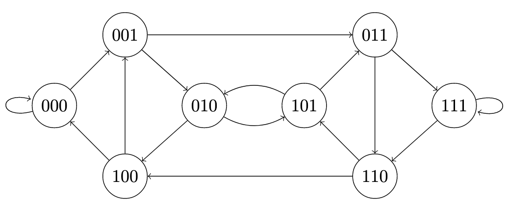
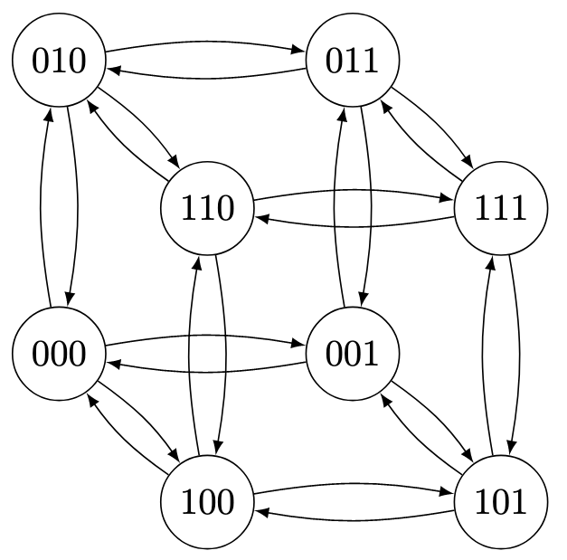
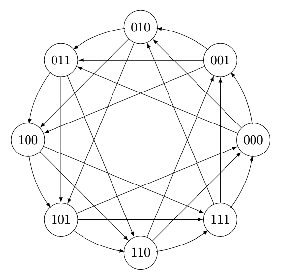
Figure 2: Various types of Markov transition graphs

So far, we have assumed the GAN training is able to find the optimal parameters for the discriminator and the generator. However, there is no guarantee that this is indeed the case with gradient updates such as Eq. (3). To analyze the behaviour of the GAN training dynamic for ASR-U, we follow prior works on neural tangent kernel (NTK) Jacot et al. (2018) to focus on the infinite-width, continuous-time regime, or NTK regime, where the generator and the discriminator are assumed to be neural networks with an infinite number of hidden neurons trained with gradient descent at an infinitely small learning rate. Though highly idealized, studying such a regime is practically useful as results from this regime can often be converted to finite-width, discrete-time settings (See, e.g., Du et al. (2019)).

For simplicity, denote fτ:=Dϕτassignsubscript𝑓𝜏subscript𝐷subscriptitalic-ϕ𝜏f_{\tau}:=D_{\phi_{\tau}} and gt:=Gθtassignsubscript𝑔𝑡subscript𝐺subscript𝜃𝑡g_{t}:=G_{\theta_{t}} and define t(f):=J(gt,f)assignsubscript𝑡𝑓𝐽subscript𝑔𝑡𝑓\mathcal{L}_{t}(f):=J(g_{t},f), then in the NTK regime, between each generator step, the training dynamic of the discriminator can be described by the following partial differential equation (PDE):

τϕτ=ϕτt(fτ).subscript𝜏subscriptitalic-ϕ𝜏subscriptsubscriptitalic-ϕ𝜏subscript𝑡subscript𝑓𝜏\displaystyle\partial_{\tau}\phi_{\tau}=\nabla_{\phi_{\tau}}\mathcal{L}_{t}(f_{\tau}). (11)

Let fPt=limτfτsuperscriptsubscript𝑓subscript𝑃𝑡subscript𝜏subscript𝑓𝜏f_{P_{t}}^{*}=\lim_{\tau\rightarrow\infty}f_{\tau} be the limit of Eq. (11). If the limit exists and is unique, the generator loss is well-defined as 𝒞t(gt):=J(gt,fPt)assignsubscript𝒞𝑡subscript𝑔𝑡𝐽subscript𝑔𝑡superscriptsubscript𝑓subscript𝑃𝑡\mathcal{C}_{t}(g_{t}):=J(g_{t},f_{P_{t}}^{*}). Note that the output of the ASR-U generator is discrete, which is not a differentiable function per se, but we can instead directly parameterize the generated text distribution as Pgt:=PXOtassignsubscript𝑃subscript𝑔𝑡subscript𝑃𝑋subscript𝑂𝑡P_{g_{t}}:=P_{X}\circ O_{t} for some softmax posterior distribution Otsubscript𝑂𝑡O_{t}:

Ot,x(y):=l=1Lexp(hθ,yl(xl))ylexp(hθ,yl(xl)),assignsubscript𝑂𝑡𝑥𝑦superscriptsubscriptproduct𝑙1𝐿subscript𝜃subscript𝑦𝑙subscript𝑥𝑙subscriptsuperscriptsubscript𝑦𝑙subscript𝜃superscriptsubscript𝑦𝑙subscript𝑥𝑙\displaystyle O_{t,x}(y):=\prod_{l=1}^{L}\frac{\exp(h_{\theta,y_{l}}(x_{l}))}{\sum_{y_{l}^{\prime}}\exp(h_{\theta,y_{l}^{\prime}}(x_{l}))}, (12)

where hθsubscript𝜃h_{\theta} is a neural network, and is assumed to be one layer in our analysis, though it can be extended to multiple layers with slight modifications using techniques similar to those in Du et al. (2019).

Using such a generator, the generator dynamic can be then described by the following PDE:

tθtsubscript𝑡subscript𝜃𝑡\displaystyle\partial_{t}\theta_{t} =y𝕐Lb(fgt(y))θtPgt(y),absentsubscript𝑦superscript𝕐𝐿𝑏subscriptsuperscript𝑓subscript𝑔𝑡𝑦subscriptsubscript𝜃𝑡subscript𝑃subscript𝑔𝑡𝑦\displaystyle=\sum_{y\in{\mathbb{Y}}^{L}}b(f^{*}_{g_{t}}(y))\nabla_{\theta_{t}}P_{g_{t}}(y), (13)

where the right-hand side is the term in the gradient of 𝒞tsubscript𝒞𝑡\mathcal{C}_{t} with respect to θtsubscript𝜃𝑡\theta_{t} ignoring the dependency of the discriminator fgtsuperscriptsubscript𝑓subscript𝑔𝑡f_{g_{t}}^{*}. Define the NTKs of the discriminator and the generator (distribution) as

Kfτ(y,y)subscript𝐾subscript𝑓𝜏𝑦superscript𝑦\displaystyle K_{f_{\tau}}(y,y^{\prime}) =𝔼ϕ0𝒲[fτ(y)ϕτfτ(y)ϕτ]absentsubscript𝔼similar-tosubscriptitalic-ϕ0𝒲delimited-[]superscriptsubscript𝑓𝜏𝑦subscriptitalic-ϕ𝜏topsubscript𝑓𝜏superscript𝑦subscriptitalic-ϕ𝜏\displaystyle=\mathbb{E}_{\phi_{0}\sim{\mathcal{W}}}\left[\frac{\partial f_{\tau}(y)}{\partial\phi_{\tau}}^{\top}\frac{\partial f_{\tau}(y^{\prime})}{\partial\phi_{\tau}}\right] (14)
Kgt(y,y)subscript𝐾subscript𝑔𝑡𝑦superscript𝑦\displaystyle K_{g_{t}}(y,y^{\prime}) =𝔼θ0𝒲[Pgt(y)θtPgt(y)θt],absentsubscript𝔼similar-tosubscript𝜃0𝒲delimited-[]superscriptsubscript𝑃subscript𝑔𝑡𝑦subscript𝜃𝑡topsubscript𝑃subscript𝑔𝑡superscript𝑦subscript𝜃𝑡\displaystyle=\mathbb{E}_{\theta_{0}\sim{\mathcal{W}}}\left[\frac{\partial P_{g_{t}}(y)}{\partial\theta_{t}}^{\top}\frac{\partial P_{g_{t}}(y^{\prime})}{\partial\theta_{t}}\right], (15)

where 𝒲𝒲{\mathcal{W}} is the initialization distribution (usually Gaussian).

Note that the NTKs are |𝕐|L×|𝕐|Lsuperscript𝕐𝐿superscript𝕐𝐿|{\mathbb{Y}}|^{L}\times|{\mathbb{Y}}|^{L} matrices for ASR-U due to the discrete nature of the generator. A key result in Jacot et al. (2018) states that as the widths of the hidden layers of the discriminator and generator go to infinity, KfτKD,KgtKGformulae-sequencesubscript𝐾subscript𝑓𝜏subscript𝐾𝐷subscript𝐾subscript𝑔𝑡subscript𝐾𝐺K_{f_{\tau}}\rightarrow K_{D},K_{g_{t}}\rightarrow K_{G} stay constant during gradient descent/ascent and we have

τfτ=KDsubscript𝜏subscript𝑓𝜏subscript𝐾𝐷\displaystyle\partial_{\tau}f_{\tau}=K_{D} (diag(PY)fτa\displaystyle\left(\mathrm{diag}(P_{Y})\nabla_{f_{\tau}}a\right.
diag(Pgt)fτb),\displaystyle\left.-\mathrm{diag}(P_{g_{t}})\nabla_{f_{\tau}}b\right), (16)
tPgt=KGsubscript𝑡subscript𝑃subscript𝑔𝑡subscript𝐾𝐺\displaystyle\partial_{t}P_{g_{t}}=K_{G} 𝐛fgt,subscript𝐛subscript𝑓subscript𝑔𝑡\displaystyle\mathbf{b}_{f_{g_{t}}}, (17)

where f{a,b}=[{a,b}(f(y))f(y)]y𝕐Lsubscript𝑓𝑎𝑏subscriptdelimited-[]𝑎𝑏𝑓𝑦𝑓𝑦𝑦superscript𝕐𝐿\nabla_{f}\{a,b\}=\left[\frac{\partial\{a,b\}(f(y))}{\partial f(y)}\right]_{y\in\mathbb{Y}^{L}} and 𝐛f=(bf(y))y𝕐Lsubscript𝐛𝑓subscriptsubscript𝑏𝑓𝑦𝑦superscript𝕐𝐿\mathbf{b}_{f}=(b_{f}(y))_{y\in{\mathbb{Y}}^{L}}.

However, Eq. (16)-(17) is in general highly nonlinear and it remains an open problem as to their convergence properties. Instead, we focus on the case when the discriminator ftsubscript𝑓𝑡f_{t} is decomposable with components ft,l,l=1,,Lformulae-sequencesubscript𝑓𝑡𝑙𝑙1𝐿f_{t,l},l=1,\cdots,L, and simplify Eq. (16) and Eq. (17) into PDEs involving only samples at a particular time step:

τfτ,l=subscript𝜏subscript𝑓𝜏𝑙absent\displaystyle\partial_{\tau}f_{\tau,l}= KD,l(diag(PlY)fτ,l𝐚fτ,l\displaystyle K_{D,l}\left(\mathrm{diag}(P^{Y}_{l})\nabla_{f_{\tau,l}}\mathbf{a}_{f_{\tau,l}}\right.
diag(Plgt)fτ,l𝐛fτ,l),\displaystyle-\left.\mathrm{diag}(P^{g_{t}}_{l})\nabla_{f_{\tau,l}}\mathbf{b}_{f_{\tau,l}}\right), (18)
tOt,x=subscript𝑡superscriptsubscript𝑂𝑡𝑥topabsent\displaystyle\partial_{t}O_{t,x}^{\top}= l=1LPlX(x)KOt,x𝐛fgt,l,superscriptsubscript𝑙1𝐿subscriptsuperscript𝑃𝑋𝑙𝑥subscript𝐾subscript𝑂𝑡𝑥subscript𝐛subscript𝑓subscript𝑔𝑡𝑙\displaystyle\sum_{l=1}^{L}P^{X}_{l}(x)K_{O_{t,x}}\mathbf{b}_{f_{g_{t},l}}, (19)

for all l=1,,L,x𝕏formulae-sequence𝑙1𝐿𝑥𝕏l=1,\cdots,L,\,x\in{\mathbb{X}} in terms of the stepwise NTKs defined as:

KD,l(y,y)subscript𝐾𝐷𝑙𝑦superscript𝑦\displaystyle K_{D,l}(y,y^{\prime}) :=𝔼ϕ0𝒲[fτ(y)ϕτfτ(y)ϕτ]assignabsentsubscript𝔼similar-tosubscriptitalic-ϕ0𝒲delimited-[]superscriptsubscript𝑓𝜏𝑦subscriptitalic-ϕ𝜏topsubscript𝑓𝜏superscript𝑦subscriptitalic-ϕ𝜏\displaystyle:=\mathbb{E}_{\phi_{0}\sim{\mathcal{W}}}\left[\frac{\partial f_{\tau}(y)}{\partial\phi_{\tau}}^{\top}\frac{\partial f_{\tau}(y^{\prime})}{\partial\phi_{\tau}}\right]
KOt,x(y,y)subscript𝐾subscript𝑂𝑡𝑥𝑦superscript𝑦\displaystyle K_{O_{t,x}}(y,y^{\prime}) :=𝔼θ0𝒲[Ot,x(y)θτOt,x(y)θτ].assignabsentsubscript𝔼similar-tosubscript𝜃0𝒲delimited-[]superscriptsubscript𝑂𝑡𝑥𝑦subscript𝜃𝜏topsubscript𝑂𝑡𝑥superscript𝑦subscript𝜃𝜏\displaystyle:=\mathbb{E}_{\theta_{0}\sim{\mathcal{W}}}\left[\frac{\partial O_{t,x}(y)}{\partial\theta_{\tau}}^{\top}\frac{\partial O_{t,x}(y^{\prime})}{\partial\theta_{\tau}}\right].

We further focus on the special case that fτ,lsubscript𝑓𝜏𝑙f_{\tau,l} is parameterized by a two-layer neural network with ReLU activation, though the framework can be extended to network of arbitrary depths:

fτ,l(y)=limm1mr=1mvrlmax{Wryl,0}.subscript𝑓𝜏𝑙𝑦subscript𝑚1𝑚superscriptsubscript𝑟1𝑚subscriptsuperscript𝑣𝑙𝑟subscriptsuperscript𝑊𝑙𝑟𝑦0\displaystyle f_{\tau,l}(y)=\lim_{m\rightarrow\infty}\frac{1}{\sqrt{m}}\sum_{r=1}^{m}v^{l}_{r}\max\{W^{l}_{ry},0\}. (20)

In this case, under mild regularity conditions, we can show that the generator trained with the alternate gradient method minimizes Eq. (8), which under the same condition as in Section 3.2, implies ASR-U is feasible.

Theorem 4.

Suppose the following assumptions hold:

  1. 1.

    The discriminator is decomposable and parameterized by Eq. (20), whose parameters are all initialized by standard Gaussian variables;

  2. 2.

    The generator is linear before the softmax layer;

  3. 3.

    The GAN objective is MMD;

  4. 4.

    The linear equation PXO=PYsuperscript𝑃𝑋𝑂superscript𝑃𝑌P^{X}O=P^{Y} has at least one solution.

Then we have for any solution Otsubscript𝑂𝑡O_{t} of Eq. (19), limtPXOt=PYsubscript𝑡superscript𝑃𝑋subscript𝑂𝑡superscript𝑃𝑌\lim_{t\rightarrow\infty}P^{X}O_{t}=P^{Y}.

4 Experiments

Refer to caption
(a) Circulant graph
Refer to caption
(b) De Bruijn graph
Refer to caption
(c) Hypercube
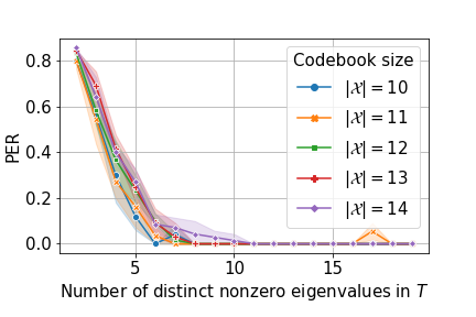
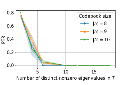
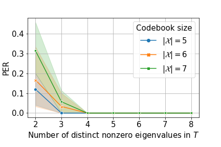
Figure 3: Asymptotic ASR-U PER vs number of distinct nonzero eigenvalues for various Markov transition graphs
Refer to caption
(a) Circulant graph
Refer to caption
(b) De Bruijn graph
Refer to caption
(c) Hypercube
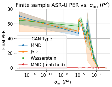
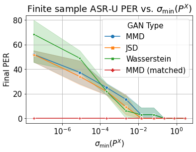
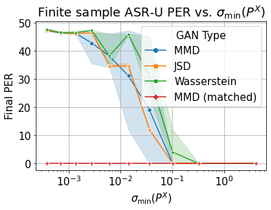
Figure 4: Finite-sample ASR-U PER vs σmin(PX)subscript𝜎superscript𝑃𝑋\sigma_{\min}(P^{X}) for various Markov transition graphs
Refer to caption
Figure 5: Effect of discriminator resetting at every update
Refer to caption
Figure 6: Effect of different type of averaging for the generator

Synthetic language dataset

To allow easy control of the eigenvalue spacings of the transition matrix T𝑇T and thus observe the phase transition phenomena predicted by our theory, we design six synthetic languages with HMM language models as follows. First, we create the HMM transition graph by treating non-overlapping bigrams as hidden states of the HMM. The hidden state of the HMM will henceforth be referred to as the “speech unit”, while the observation emitted by the HMM will be referred to as the “text unit”. For the asymptotic ASR-U, we control the number of eigenvalues of the Markov transition graph by varying the number of disjoint, identical subgraphs. The number of distinct eigenvalues of the whole graph will then be equal to the number of eigenvalues of each subgraph. For the finite sample setting, we instead select only Hamiltonian graphs and either gradually decrease the degrees of the original graph to its Hamiltonian cycle or interpolate between the graph adjacency matrix and that of its Hamiltonian cycle. Thus, we can increase σmin(PX)subscript𝜎superscript𝑃𝑋\sigma_{\min}(P^{X}) by increasing w𝑤w. For both the subgraph in the former case and the Hamiltonian graph in the latter, we experiments with circulant, de Bruijn graphs de Bruijn (1946) and hypercubes, as illustrated in Figure 2. Next, we randomly permute the hidden state symbols to form the true generator mapping from the speech units to text units. To create matched speech-text data, we simply sample matched speech and text unit sequences using a single HMM. For unmatched datasets, we sample the speech and text data independently with two HMMs with the same parameters. Please refer to Appendix B for more details.

Model architecture

For finite-sample ASR-U, we use wav2vec-U Baevski et al. (2021) with several modifications. In particular, we experiment with various training objectives other than the Jensen-Shannon (JS) GAN used in the original wav2vec-U, including the Wasserstein GAN Liu et al. (2018) and the MMD GAN. All additional regularization losses are disabled. Moreover, we experimentally manipulate two hyperparameters: (1) the averaging strategy used by the generator, and (2) whether to reset the discriminator weights to zero at the beginning of each discriminator training loop. More details can be found in Appendix B.

Phase transition of PER vs. eigenvalue gaps: asymptotic case

The phoneme error rate (PER) as a function of the number of eigenvalues of A𝐴A for the asymptotic ASR-U on the synthetic datasets are shown in Figure 3. For all three graphs, we observe clear phase transitions as the number of eigenvalues exceeds the number of speech units, and an increase of the number of distinct, nonzero eigenvalues required for perfect ASR-U as the number of speech units increases.

Phase transition of PER vs. eigenvalue gaps: finite-sample case

The PER as a function of the least singular value σmin(PX)subscript𝜎superscript𝑃𝑋\sigma_{\min}(P^{X}) for the finite-sample ASR-U on the synthetic datasets are shown in Figure 4. As we can see, the ASR-U exhibit the phase transition phenomena in all three graphs, albeit with differences in the critical point and their rate of approaching the perfect ASR-U regime. While the PER generally decreases as σmin(PX)subscript𝜎superscript𝑃𝑋\sigma_{\min}(P^{X}) gets larger, we found a dip in PER in the circulant graph case as σmin(PX)subscript𝜎superscript𝑃𝑋\sigma_{\min}(P^{X}) moves from 1031superscript103110^{-31} to 1015superscript101510^{-15}. Though unexpected, this observation is not contradictory to our theory since our theory does not make explicit predictions about the rate of phase transition for ASR-U. Across different GAN models, we found that JSD generally approaches perfect ASR-U at a faster rate than MMD in all three graphs, suggesting the use of nonlinear dynamic may be beneficial. Nevertheless, the overall trends for different GANs remain in large part homogeneous. Between Wasserstein and MMD, we observe very little difference in performance, suggesting the regularization effect of NTK is sufficient to control the Lipschitz coefficient of the network. Finally, for the MMD GAN in the matched setting, we found the network is able to achieve perfect ASR-U regardless of the spectral properties of the Markov transition graphs, which confirms our theory that a symmetric Markov random matrix tends to have simple eigenvalue spectrum suitable for ASR-U.

Effect of discriminator reset

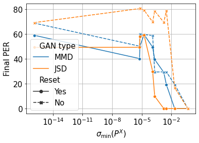
As pointed out by Franceschi et al. (2021), a discriminator may suffer from residual noise from previous updates and fail to approximate the target divergence measure. We analyze such effects for MMD and JSD as shown in Figure 5. We observed consistent trends that models whose weights are reset to the initial weights every discriminator loop outperform those without resetting. The effect is more pronounced for JSD GAN than MMD GAN and for smaller σmin(PX)subscript𝜎superscript𝑃𝑋\sigma_{\min}(P^{X}).

Effect of generator averaging strategy

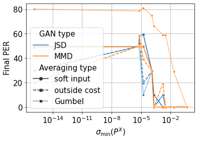
The original wav2vec-U Baevski et al. (2021) directly feeds the text posterior probabilities O𝑂O into the discriminator, which we refer to as the “soft input” approach. Alternatively, we can instead calculate a weighted average of the gradient form over the samples y𝕐L𝑦superscript𝕐𝐿y\in{\mathbb{Y}}^{L} as in Eq. (13), which we refer to as the “outside cost” approach. The comparison between the two approaches are shown in Figure 6. We observed mixed results: for MMD GANs, the soft-input approach outperforms the outside-cost approach and performs best among the models in the high-σmin(PX)subscript𝜎superscript𝑃𝑋\sigma_{\min}(P^{X}) setting; for JSD GANs, we found that the outside-cost approach performs slightly better than the soft-input approach. Such inconsistencies may be another consequence of the regularization effect predicted by the GANTK. We leave the theoretical explanation as future work.

5 Related works

Glass (2012) first proposed the challenging task of ASR-U as a key step toward unsupervised speech processing, and framed it as a decipherment problem. Liu et al. (2018) takes on the challenge by developing the first ASR-U system with ground-truth phoneme boundaries and quantized speech features as inputs, by training a GAN to match the speech-generated and real text distributions. Chen et al. (2019) later replaced the ground truth boundaries with unsupervised ones refined iteratively by an HMM, which also incorporates language model information into the system. Yeh et al. (2019) explored the cross entropy loss for matching the generated and real text distribution, but it is prone to mode collapse and needs the help of additional regularization losses such as smoothness weight. More recently, Baevski et al. (2021); Liu et al. (2022) proposed another GAN-based model using continuous features from the last hidden layer of the wav2vec 2.0 Baevski et al. (2020) model and additional regularization losses to stabilize training. Their approach achieves ASR error rates comparable to the supervised system on multiple languages, making it the current state-of-the-art system.

To better understand the learning behavior of ASR-U systems, Lin et al. (2022) analyze the robustness of wav2vec-U against empirical distribution mismatch between the speech and text, and found that N𝑁N-gram language model is predictive of the success of ASR-U. Inspired by the original framework in Glass (2012), Klejch et al. (2022) proposed a decipher-based cross-lingual ASR system by mapping IPA symbols extracted from a small amount of speech data with unpaired phonetic transcripts in the target language.

Our analysis on the sufficient condition of ASR-U is based on previous work on the asymptotic behaviour of GAN objective functions Goodfellow et al. (2014); Arjovsky et al. (2017). Our finite-sample analysis takes inspiration from later work extending the asymptotic analysis to the finite-sample regimes Arora et al. (2017); Bai et al. (2019). Such frameworks, however, do not account for the alternate gradient optimization method of GANs and inevitably lead to various inconsistencies between the theory and empirical observations of GAN training Franceschi et al. (2021). Building upon prior works Mescheder et al. (2017, 2018); Domingo-Enrich et al. (2020); Mroueh and Nguyen (2021); Balaji et al. (2021),  Franceschi et al. (2021) proposed a unified framework called GANTK based on NTK Jacot et al. (2018) to describe the training dynamic of any GAN objectives and network architectures. Our analysis on the training dynamic of ASR-U adopts and extends the GANTK framework to handle discrete, sequential data such as natural languages.

6 Conclusion

In this paper, we develop a theoretical framework to study the fundamental limits of ASR-U as well as the convergence properties of GAN-based ASR-U algorithms. In doing so, our theory sheds light on the underlying causes of training instability for such algorithms, as well as several new directions for more reliable ASR-U training.

7 Limitations

Our theory currently assumes that input speech features are quantized into discrete units, as in Chen et al. (2019), while preserving all the linguistic information in the speech. As a result, our theory does not account for the loss of linguistic information during the quantization process, as often occurred in realistic speech datasets. Further, more recent works Baevski et al. (2021); Liu et al. (2022) have shown that continuous features, with the help of additional regularization losses, can achieve almost perfect ASR-U. Such phenomena is beyond explanations based on our current theory and require generalizing our theory to continuous speech features. Further, our model assumes that sufficiently reliable phoneme boundaries are fed to the ASR-U system, and kept fixed during training. It will be interesting to extend our framework to systems with trainable phoneme boundaries, such as the wav2vec-U systems, to better understand its effect on training stability.

Acknowledgements

This work was supported by Institute of Information & communications Technology Planning & Evaluation (IITP) grant funded by the Korea government(MSIT) (No.2022-0-00184, Development and Study of AI Technologies to Inexpensively Conform to Evolving Policy on Ethics)

References

Appendix A Proofs of theoretical results

A.1 Learnability of ASR-U: a sufficient condition

Proof.

(Theorem 1)

For simplicity, we assume that the eigenvalues of A𝐴A are real though a similar argument applies to complex eigenvalues as well. By Assumptions 1 and 2, it can be verified that

PXkNsubscript𝑃subscript𝑋𝑘𝑁\displaystyle P_{X_{kN}} =πAkEabsentsuperscript𝜋topsuperscript𝐴𝑘𝐸\displaystyle=\pi^{\top}A^{k}E
=πUΛkU1E,absentsuperscript𝜋top𝑈superscriptΛ𝑘superscript𝑈1𝐸\displaystyle=\pi^{\top}U\Lambda^{k}U^{-1}E,

where E=𝟏|𝕏|N2I|𝕏|𝐸tensor-productsubscript1superscript𝕏𝑁2subscript𝐼𝕏E=\mathbf{1}_{|{\mathbb{X}}|^{N-2}}\otimes I_{|{\mathbb{X}}|}, where tensor-product\otimes denotes the Kronecker product. Define cjk=πujksubscript𝑐𝑗𝑘superscript𝜋topsubscript𝑢𝑗𝑘c_{jk}=\pi^{\top}u_{jk}. Define rjksuperscriptsubscript𝑟𝑗𝑘topr_{jk}^{\top} to be the kthsuperscript𝑘thk^{\textrm{th}} row of the jthsuperscript𝑗thj^{\textrm{th}} block of the matrix U1Esuperscript𝑈1𝐸U^{-1}E, i.e., UU1E=j=1Kk=1Njujkrjk𝑈superscript𝑈1𝐸superscriptsubscript𝑗1𝐾superscriptsubscript𝑘1subscript𝑁𝑗subscript𝑢𝑗𝑘superscriptsubscript𝑟𝑗𝑘topUU^{-1}E=\sum_{j=1}^{K}\sum_{k=1}^{N_{j}}u_{jk}r_{jk}^{\top}. Define the matrix RKsubscript𝑅𝐾R_{K} as RK=[r1,,rK]subscript𝑅𝐾subscript𝑟1subscript𝑟𝐾R_{K}=[r_{1},\cdots,r_{K}], where rj=k=1Njcjkrjksubscript𝑟𝑗superscriptsubscript𝑘1subscript𝑁𝑗subscript𝑐𝑗𝑘subscript𝑟𝑗𝑘r_{j}=\sum_{k=1}^{N_{j}}c_{jk}r_{jk}. Then we have:

PXkNsuperscriptsubscript𝑃subscript𝑋𝑘𝑁top\displaystyle P_{X_{kN}}^{\top} =j=1Kλjkrjabsentsuperscriptsubscript𝑗1𝐾subscriptsuperscript𝜆𝑘𝑗superscriptsubscript𝑟𝑗top\displaystyle=\sum_{j=1}^{K}\lambda^{k}_{j}r_{j}^{\top}
PXsuperscript𝑃𝑋\displaystyle P^{X} =VL(λ1:K)RK,absentsubscript𝑉𝐿superscriptsubscript𝜆:1𝐾topsuperscriptsubscript𝑅𝐾top\displaystyle=V_{L}(\lambda_{1:K})^{\top}R_{K}^{\top},

where VL(λ1:K)subscript𝑉𝐿subscript𝜆:1𝐾V_{L}(\lambda_{1:K}) is the Vandermonde matrix formed by nonzero eigenvalues λ1,,λKsubscript𝜆1subscript𝜆𝐾\lambda_{1},\cdots,\lambda_{K} and with L𝐿L columns, K|𝕏|𝐾𝕏K\geq|{\mathbb{X}}| by Assumption 1. RKsubscript𝑅𝐾R_{K} has full column rank of K|X|𝐾𝑋K\geq|X| by Assumption 2, therefore it is possible to write RK=R^KLsubscript𝑅𝐾subscript^𝑅𝐾𝐿R_{K}=\hat{R}_{K}L, where R^K=r^1,,r^K]\hat{R}_{K}=\hat{r}_{1},\ldots,\hat{r}_{K}] is a matrix with orthogonal columns, and L𝐿L is lower-triangular. As a result, we have PXsuperscript𝑃𝑋P^{X} is full rank iff VL(λ1:K)subscript𝑉𝐿subscript𝜆:1𝐾V_{L}(\lambda_{1:K}) has full row rank of at least |𝕏|𝕏|{\mathbb{X}}|, which holds by Assumption 1. ∎

Proof.

(Lemma 1)

Use the Rayleigh-characterization of eigenvalues of the matrix PXPXsuperscript𝑃limit-from𝑋topsuperscript𝑃𝑋P^{X\top}P^{X}, we have

σmin(PX)subscript𝜎superscript𝑃𝑋\displaystyle\sigma_{\min}(P^{X})
=λmin(PXPX)absentsubscript𝜆superscript𝑃limit-from𝑋topsuperscript𝑃𝑋\displaystyle=\sqrt{\lambda_{\min}(P^{X\top}P^{X})}
=minw=1wPXPXwabsentsubscriptnorm𝑤1superscript𝑤topsuperscript𝑃limit-from𝑋topsuperscript𝑃𝑋𝑤\displaystyle=\sqrt{\min_{\|w\|=1}w^{\top}P^{X\top}P^{X}w}
=minw=1wRKVLVLRKwabsentsubscriptnorm𝑤1superscript𝑤topsubscript𝑅𝐾subscript𝑉𝐿superscriptsubscript𝑉𝐿topsuperscriptsubscript𝑅𝐾top𝑤\displaystyle=\sqrt{\min_{\|w\|=1}w^{\top}R_{K}V_{L}V_{L}^{\top}R_{K}^{\top}w}
l=0L|𝕏|1λmin2lminw=1wRKV|𝕏|V|𝕏|RKwabsentsuperscriptsubscript𝑙0𝐿𝕏1superscriptsubscript𝜆2𝑙subscriptnorm𝑤1superscript𝑤topsubscript𝑅𝐾subscript𝑉𝕏superscriptsubscript𝑉𝕏topsuperscriptsubscript𝑅𝐾top𝑤\displaystyle\geq\sqrt{\sum_{l=0}^{L-|{\mathbb{X}}|-1}\lambda_{\min}^{2l}\min_{\|w\|=1}w^{\top}R_{K}V_{|{\mathbb{X}}|}V_{|{\mathbb{X}}|}^{\top}R_{K}^{\top}w}
=σmin(P1:|𝕏|X)l=0L|𝕏|1λmin2l,absentsubscript𝜎subscriptsuperscript𝑃𝑋:1𝕏superscriptsubscript𝑙0𝐿𝕏1superscriptsubscript𝜆2𝑙\displaystyle=\sigma_{\min}(P^{X}_{1:|{\mathbb{X}}|})\sqrt{\sum_{l=0}^{L-|{\mathbb{X}}|-1}\lambda_{\min}^{2l}},

where λminsubscript𝜆\lambda_{\min} is the eigenvalue of A𝐴A with minimum absolute value, and P1:|𝕏|Xsubscriptsuperscript𝑃𝑋:1𝕏P^{X}_{1:|{\mathbb{X}}|} is the first |𝕏|𝕏|{\mathbb{X}}| rows of PXsuperscript𝑃𝑋P^{X}. Therefore, to lower bound σmin(PX)subscript𝜎superscript𝑃𝑋\sigma_{\min}(P^{X}), it suffices to lower bound σmin(P1:|𝕏|X)subscript𝜎subscriptsuperscript𝑃𝑋:1𝕏\sigma_{\min}(P^{X}_{1:|{\mathbb{X}}|}). But note that

σmin(P1:|𝕏|X)subscript𝜎subscriptsuperscript𝑃𝑋:1𝕏\displaystyle\sigma_{\min}(P^{X}_{1:|{\mathbb{X}}|})
=\displaystyle= minw=1V|𝕏|TRKTwsubscriptnorm𝑤1normsuperscriptsubscript𝑉𝕏𝑇superscriptsubscript𝑅𝐾𝑇𝑤\displaystyle\min_{\|w\|=1}\|V_{|{\mathbb{X}}|}^{T}R_{K}^{T}w\|
\displaystyle\geq σmin(V|𝕏|T)minw=1RKTwsubscript𝜎superscriptsubscript𝑉𝕏𝑇subscriptnorm𝑤1normsuperscriptsubscript𝑅𝐾𝑇𝑤\displaystyle\sigma_{\min}(V_{|{\mathbb{X}}|}^{T})\min_{\|w\|=1}\|R_{K}^{T}w\|
\displaystyle\geq σmax(V|𝕏|)κ(V|𝕏|)minjr^jsubscript𝜎subscript𝑉𝕏𝜅subscript𝑉𝕏subscript𝑗normsubscript^𝑟𝑗\displaystyle\frac{\sigma_{\max}(V_{|{\mathbb{X}}|})}{\kappa(V_{|{\mathbb{X}}|})}\min_{j}\|\hat{r}_{j}\|
\displaystyle\geq |det(V|𝕏|)|1/|𝕏|κ(V|𝕏|)minjr^jsuperscriptsubscript𝑉𝕏1𝕏𝜅subscript𝑉𝕏subscript𝑗normsubscript^𝑟𝑗\displaystyle\frac{|\det(V_{|{\mathbb{X}}|})|^{1/|{\mathbb{X}}|}}{\kappa(V_{|{\mathbb{X}}|})}\min_{j}\|\hat{r}_{j}\|
=\displaystyle= |1i<j|𝕏||λiλj|1/|𝕏|κ(V|𝕏|)minjr^j\displaystyle\frac{|\prod_{1\leq i<j\leq|{\mathbb{X}}|}|\lambda_{i}-\lambda_{j}|^{1/|{\mathbb{X}}|}}{\kappa(V_{|{\mathbb{X}}|})}\min_{j}\|\hat{r}_{j}\|
\displaystyle\geq δmin(|𝕏|1)/2|𝕏|κ(V|𝕏|)minjr^jsuperscriptsubscript𝛿𝕏12𝕏𝜅subscript𝑉𝕏subscript𝑗normsubscript^𝑟𝑗\displaystyle\frac{\delta_{\min}^{(|{\mathbb{X}}|-1)/2|{\mathbb{X}}|}}{\kappa(V_{|{\mathbb{X}}|})}\min_{j}\|\hat{r}_{j}\|

where the last equality uses the closed-form formula of the determinant of a square Vandermonde matrix, and where the behaviour of κ(V|𝕏|)𝜅subscript𝑉𝕏\kappa(V_{|{\mathbb{X}}|}), the condition number of the Vandermonde matrix, has been studied in depth in Bazán (2000). ∎

A.2 Finite-sample learnability of ASR-U: matched setup

Theory of small ball probability

The proof of Theorem 2 makes extensive use of the theory of small ball probability. Therefore, we briefly provide some background on the subject. First, we define the small ball probability of a vector x𝑥x as follows.

Definition 2.

(Small ball probability) Given a fixed vector x=(x1,,xn)𝑥subscript𝑥1subscript𝑥𝑛x=(x_{1},\cdots,x_{n}), and i.i.d random variables ξ=(ξi,,ξn)𝜉subscript𝜉𝑖subscript𝜉𝑛\xi=(\xi_{i},\cdots,\xi_{n}), the small ball probability is defined as

ρδ(x):=supaPr[|ξxa|δ].assignsubscript𝜌𝛿𝑥subscriptsupremum𝑎Prsuperscript𝜉top𝑥𝑎𝛿\displaystyle\rho_{\delta}(x):=\sup_{a\in{\mathbb{R}}}\Pr[|\xi^{\top}x-a|\leq\delta].

Intuitively, small ball probability is the amount of “additive structure” in x𝑥x: for example, if the coordinates of x𝑥x are integer multiples of each other and ξisubscript𝜉𝑖\xi_{i}’s are symmetric Bernoulli variables, the product ξxsuperscript𝜉top𝑥\xi^{\top}x tends to have small magnitude as terms cancel out each other very often. Since sparser vectors tend to have less additive structure, small ball probability can also be used to measure how sparse the weights of x𝑥x are. Another way to look at this is that, if the L2 norm of x𝑥x is fixed and most of the weight of x𝑥x is gathered in a few coordinates, the product ξxsuperscript𝜉top𝑥\xi^{\top}x has higher variance and is thus less likely to settle in any fixed-length intervals. This is quantitatively captured by the celebrated Offord-Littlewood-Erdös (OLE) anti-concentration inequality (and its inverse) for general subgaussian random variables:

Lemma 2.

Erdös (1945); Rudelson and Vershynin (2008); Tao and Vu (2009) Let ϵ>0italic-ϵ0\epsilon>0 be fixed, let δ>0𝛿0\delta>0, and let vm𝑣superscript𝑚v\in{\mathbb{R}}^{m} be a unit vector with

ρδ(v)m12+ϵ.subscript𝜌𝛿𝑣superscript𝑚12italic-ϵ\displaystyle\rho_{\delta}(v)\geq m^{-\frac{1}{2}+\epsilon}.

Then all but at most ϵmitalic-ϵ𝑚\epsilon m of the coefficients of v𝑣v have magnitude at most δ𝛿\delta.

Note that here we use a slight generalization of the notion of sparsity called compressibility defined as follows.

Definition 3.

((α,δ)𝛼𝛿(\alpha,\delta)-compressible) A vector vn𝑣superscript𝑛v\in{\mathbb{R}}^{n} is (α,δ)𝛼𝛿(\alpha,\delta)-compressible if at most αn𝛼𝑛\lfloor\alpha n\rfloor of its coefficients have magnitude above δ𝛿\delta.

Note that a sparse vector with a support of size at most αn𝛼𝑛\lfloor\alpha n\rfloor is (α,0)𝛼0(\alpha,0)-compressible.

A more generally applicable anti-concentration inequality requires the following definition of generalized arithmetic progression, which is used to quantify the amount of additive structure of a vector.

Definition 4.

(Generalized arithmetic progression) A generalized arithmetic progression (GAP) is a set of the form

Q={aw:ar,|ai|Ni,1ir},𝑄conditional-setsuperscript𝑎top𝑤formulae-sequence𝑎superscript𝑟formulae-sequencesubscript𝑎𝑖subscript𝑁𝑖1𝑖𝑟\displaystyle Q=\{a^{\top}w:a\in{\mathbb{Z}}^{r},|a_{i}|\leq N_{i},1\leq i\leq r\},

where r0𝑟0r\geq 0 is called the rank of the GAP and w1,,wrsubscript𝑤1subscript𝑤𝑟w_{1},\cdots,w_{r}\in{\mathbb{R}} are called generators of the GAP. Further, the quantity

vol(Q):=i=1r(2Ni+1)assignvol𝑄superscriptsubscriptproduct𝑖1𝑟2subscript𝑁𝑖1\displaystyle\mathrm{vol}(Q):=\prod_{i=1}^{r}(2N_{i}+1)

is called the volume of the GAP.

Lemma 3.

(Continuous inverse Littlewood-Offord theorem, Theorem 2.9 of Nguyen and Vu (2011)) Let ϵ>0italic-ϵ0\epsilon>0 be fixed, let δ>0𝛿0\delta>0 and let vn𝑣superscript𝑛v\in{\mathbb{R}}^{n} be a unit vector whose small ball probability ρ:=ρδ(v)assign𝜌subscript𝜌𝛿𝑣\rho:=\rho_{\delta}(v) obeys the lower bound

ρnO(1).much-greater-than𝜌superscript𝑛𝑂1\displaystyle\rho\gg n^{-O(1)}.

Then there exists a generalized arithmetic progression Q𝑄Q of volume

vol(Q)max(O(1ραn),1)𝑣𝑜𝑙𝑄𝑂1𝜌𝛼𝑛1\displaystyle vol(Q)\leq\max\left(O\left(\frac{1}{\rho\sqrt{\alpha n}}\right),1\right)

such that all but at most αn𝛼𝑛\alpha n of the coefficients v1,,vnsubscript𝑣1subscript𝑣𝑛v_{1},\cdots,v_{n} of v𝑣v lie within δ𝛿\delta of Q. Furthermore, if r𝑟r denotes the rank of Q𝑄Q, then r=O(1)𝑟𝑂1r=O(1) and all the generators w1,,wrsubscript𝑤1subscript𝑤𝑟w_{1},\cdots,w_{r} of Q𝑄Q have magnitude O(1)𝑂1O(1).

While applicable for any ρnϵmuch-greater-than𝜌superscript𝑛italic-ϵ\rho\gg n^{-\epsilon} rather than only those with ρδ(v)n1/2+ϵsubscript𝜌𝛿𝑣superscript𝑛12italic-ϵ\rho_{\delta}(v)\geq n^{-1/2+\epsilon} as required by Lemma 2, Lemma 3 is weaker than Lemma 2 in the sense that rather than showing that the vector is compressible with high probability and thus covered by the set of compressible vectors, it proves that the vector is covered by a small set with high probability.

A related notion that is often more convenient for our analysis is the segmental small ball probability, which is simply small ball probability computed on a segment of the vector:

ρδ,α(x)=infI{1,,n}:|I|=αnρδ(xI),subscript𝜌𝛿𝛼𝑥subscriptinfimum:𝐼1𝑛𝐼𝛼𝑛subscript𝜌𝛿subscript𝑥𝐼\displaystyle\rho_{\delta,\alpha}(x)=\inf_{I\subseteq\{1,\cdots,n\}:|I|=\lfloor\alpha n\rfloor}\rho_{\delta}(x_{I}),

From the definition, it is not hard to see that ρδ,α(x)ρδ(x)subscript𝜌𝛿𝛼𝑥subscript𝜌𝛿𝑥\rho_{\delta,\alpha}(x)\geq\rho_{\delta}(x).

Eigen-gaps of symmetric Markov random matrix

Armed with tools from the theory of small ball probability, we will establish guarantees of eigenvalue gaps for a symmetric Markov random matrix. First, we shall show that Theorem 2 implies Corollary 1.

Proof.

(Proof of Corollary 1) Using Theorem 2 and union bound, the probability that a symmetric Markov random matrix has at least |𝕏|𝕏|{\mathbb{X}}| distinct eigenvalues can be bounded as

Pr[min1i|𝕏||λiλi+1||𝕏|BN]Prsubscript1𝑖𝕏subscript𝜆𝑖subscript𝜆𝑖1superscript𝕏𝐵𝑁absent\displaystyle\Pr\left[\min_{1\leq i\leq|{\mathbb{X}}|}|\lambda_{i}-\lambda_{i+1}|\leq|{\mathbb{X}}|^{-BN}\right]\leq
|𝕏|maxiPr[|λiλi+1||𝕏|BN]𝕏subscript𝑖Prsubscript𝜆𝑖subscript𝜆𝑖1superscript𝕏𝐵𝑁\displaystyle|{\mathbb{X}}|\max_{i}\Pr\left[|\lambda_{i}-\lambda_{i+1}|\leq|{\mathbb{X}}|^{-BN}\right]
=O(|𝕏|CN),absent𝑂superscript𝕏𝐶𝑁\displaystyle=O(|{\mathbb{X}}|^{-CN}),

with probability at least 1O(exp(α0|𝕏|N))1𝑂subscript𝛼0superscript𝕏𝑁1-O(\exp(-\alpha_{0}|{\mathbb{X}}|^{N})). ∎

It turns out that a symmetric Markov random matrix enjoys various properties analogous to a symmetric matrix. First, we can show that its eigenvalues are real. This can be proved by noting that for a symmetric Markov random matrix An:=Dn1Wnassignsubscript𝐴𝑛superscriptsubscript𝐷𝑛1subscript𝑊𝑛A_{n}:=D_{n}^{-1}W_{n} and for any of its eigenvalues λ𝜆\lambda with eigenvector v𝑣v,

Dn1Wnv=λvsuperscriptsubscript𝐷𝑛1subscript𝑊𝑛𝑣𝜆𝑣\displaystyle D_{n}^{-1}W_{n}v=\lambda v
\displaystyle\Longleftrightarrow Dn1/2WnDn1/2(Dn1/2v)=λDn1/2v,superscriptsubscript𝐷𝑛12subscript𝑊𝑛superscriptsubscript𝐷𝑛12superscriptsubscript𝐷𝑛12𝑣𝜆superscriptsubscript𝐷𝑛12𝑣\displaystyle D_{n}^{-1/2}W_{n}D_{n}^{-1/2}(D_{n}^{1/2}v)=\lambda D_{n}^{1/2}v, (21)

which implies Ansubscript𝐴𝑛A_{n} has the same spectrum as Dn1/2WnDn1/2superscriptsubscript𝐷𝑛12subscript𝑊𝑛superscriptsubscript𝐷𝑛12D_{n}^{-1/2}W_{n}D_{n}^{-1/2}, which is symmetric and thus has a real spectrum. Further, we can prove a variant of Cauchy’s interlace theorem for symmetric Markov random matrix.

Lemma 4.

Suppose An=Dn1Wnn×nsubscript𝐴𝑛subscriptsuperscript𝐷1𝑛subscript𝑊𝑛superscript𝑛𝑛A_{n}=D^{-1}_{n}W_{n}\in{\mathbb{R}}^{n\times n} is a symmetric Markov random matrix with adjacency matrix Wnsubscript𝑊𝑛W_{n} and eigenvalues λ1λnsubscript𝜆1subscript𝜆𝑛\lambda_{1}\geq\cdots\geq\lambda_{n} and Am=Dm1Wmsubscript𝐴𝑚subscriptsuperscript𝐷1𝑚subscript𝑊𝑚A_{m}=D^{-1}_{m}W_{m} with adjacency matrix Wm1subscript𝑊𝑚1W_{m-1} and eigenvalues ν1νm,m<nformulae-sequencesubscript𝜈1subscript𝜈𝑚𝑚𝑛\nu_{1}\geq\cdots\geq\nu_{m},m<n is formed by successively deleting i𝑖i-rows and i𝑖i-columns, then

λiνiλi+nm.subscript𝜆𝑖subscript𝜈𝑖subscript𝜆𝑖𝑛𝑚\displaystyle\lambda_{i}\leq\nu_{i}\leq\lambda_{i+n-m}.
Proof.

Using the previous observation in Eq. A.2, we can apply the standard Cauchy’s interlacing theorem on An:=Dn1/2WnDn1/2assignsuperscriptsubscript𝐴𝑛subscriptsuperscript𝐷12𝑛subscript𝑊𝑛subscriptsuperscript𝐷12𝑛A_{n}^{\prime}:=D^{-1/2}_{n}W_{n}D^{-1/2}_{n} and Am:=Dm1/2WmDm1/2assignsuperscriptsubscript𝐴𝑚subscriptsuperscript𝐷12𝑚subscript𝑊𝑚subscriptsuperscript𝐷12𝑚A_{m}^{\prime}:=D^{-1/2}_{m}W_{m}D^{-1/2}_{m}, then we have

λi(An)subscript𝜆𝑖subscript𝐴𝑛\displaystyle\lambda_{i}(A_{n}) =λi(An)λi(Am)=λi(Am)absentsubscript𝜆𝑖superscriptsubscript𝐴𝑛subscript𝜆𝑖superscriptsubscript𝐴𝑚subscript𝜆𝑖subscript𝐴𝑚\displaystyle=\lambda_{i}(A_{n}^{\prime})\leq\lambda_{i}(A_{m}^{\prime})=\lambda_{i}(A_{m})
λi+nm(An)=λi+nm(An).absentsubscript𝜆𝑖𝑛𝑚superscriptsubscript𝐴𝑛subscript𝜆𝑖𝑛𝑚subscript𝐴𝑛\displaystyle\leq\lambda_{i+n-m}(A_{n}^{\prime})=\lambda_{i+n-m}(A_{n}).

Next, we can show that the eigenvalues of a symmetric Markov random matrix and its adjacency matrix are simultaneously distributed within the bounded intervals [10nγ1,10nγ1]10superscript𝑛𝛾110superscript𝑛𝛾1[-10n^{\gamma-1},10n^{\gamma-1}] and [10nγ,10nγ]10superscript𝑛𝛾10superscript𝑛𝛾[-10n^{\gamma},10n^{\gamma}] with high probability. For this and subsequent proofs, we will assume γ=γ>1/2superscript𝛾𝛾12\gamma^{\prime}=\gamma>1/2.

Lemma 5.

Let An=Dn1Wnsubscript𝐴𝑛superscriptsubscript𝐷𝑛1subscript𝑊𝑛A_{n}=D_{n}^{-1}W_{n} be a symmetric Markov random matrix with adjacency matrix Wnsubscript𝑊𝑛W_{n} and properties defined in Theorem 2, then we have with probability at least 1O(exp(α0n))1𝑂subscript𝛼0𝑛1-O(\exp(-\alpha_{0}n)),

λi(An)subscript𝜆𝑖subscript𝐴𝑛\displaystyle\lambda_{i}(A_{n}) [10nγ1,10nγ1],absent10superscript𝑛𝛾110superscript𝑛𝛾1\displaystyle\in[-10n^{\gamma-1},10n^{\gamma-1}],
λi(Wn)subscript𝜆𝑖subscript𝑊𝑛\displaystyle\lambda_{i}(W_{n}) [10nγ,10nγ],absent10superscript𝑛𝛾10superscript𝑛𝛾\displaystyle\in[-10n^{\gamma},10n^{\gamma}],

for any 1in1𝑖𝑛1\leq i\leq n and some α0>0subscript𝛼00\alpha_{0}>0.

Proof.

First, by definition, we can let Wn=Fn+Xnsubscript𝑊𝑛subscript𝐹𝑛subscript𝑋𝑛W_{n}=F_{n}+X_{n}, where Fnsubscript𝐹𝑛F_{n} is a deterministic matrix with eigenvalues of order nγsuperscript𝑛𝛾n^{\gamma} and Xnsubscript𝑋𝑛X_{n} is a symmetric matrix whose elements are independent zero-mean unit-variance subgaussian random variables. Using standard results from random matrix theory Anderson et al. (2009), we have

{λ1(Xn),,λn(Xn)}[10nγ1,10nγ1],subscript𝜆1subscript𝑋𝑛subscript𝜆𝑛subscript𝑋𝑛10superscript𝑛𝛾110superscript𝑛𝛾1\displaystyle\{\lambda_{1}(X_{n}),\cdots,\lambda_{n}(X_{n})\}\subset[-10n^{\gamma-1},10n^{\gamma-1}],

with probability at least 1O(exp(α0n))1𝑂subscript𝛼0𝑛1-O(\exp(-\alpha_{0}n)). Therefore, Weyl’s matrix perturbation inequality then ensures that

{λ1(Wn),,λn(Wn)}[10nγ,10nγ],subscript𝜆1subscript𝑊𝑛subscript𝜆𝑛subscript𝑊𝑛10superscript𝑛𝛾10superscript𝑛𝛾\displaystyle\{\lambda_{1}(W_{n}),\cdots,\lambda_{n}(W_{n})\}\in[-10n^{\gamma},10n^{\gamma}],

with probability at least 1O(exp(α1n))1𝑂subscript𝛼1𝑛1-O(\exp(-\alpha_{1}n)). Suppose this event occurs and use Lemma 4 and the variational characterization of eigenvalues, we have

λi(An)subscript𝜆𝑖subscript𝐴𝑛\displaystyle\lambda_{i}(A_{n}) =minVi1maxvVi1v2=1vDn1/2WnDn1/2vabsentsubscriptsubscript𝑉𝑖1subscriptFRACOP𝑣superscriptsubscript𝑉𝑖1perpendicular-tosubscriptnorm𝑣21superscript𝑣topsuperscriptsubscript𝐷𝑛12subscript𝑊𝑛superscriptsubscript𝐷𝑛12𝑣\displaystyle=\min_{V_{i-1}}\max_{v\in V_{i-1}^{\perp}\atop\|v\|_{2}=1}v^{\top}D_{n}^{-1/2}W_{n}D_{n}^{-1/2}v
=minVi1maxvVi1vDv=1vWnvabsentsubscriptsubscript𝑉𝑖1subscriptFRACOP𝑣superscriptsubscript𝑉𝑖1perpendicular-tosuperscript𝑣top𝐷𝑣1superscript𝑣topsubscript𝑊𝑛𝑣\displaystyle=\min_{V_{i-1}}\max_{v\in V_{i-1}^{\perp}\atop v^{\top}Dv=1}v^{\top}W_{n}v
=minVi1maxvVi1vWnvvDnv,absentsubscriptsubscript𝑉𝑖1subscript𝑣superscriptsubscript𝑉𝑖1perpendicular-tosuperscript𝑣topsubscript𝑊𝑛𝑣superscript𝑣topsubscript𝐷𝑛𝑣\displaystyle=\min_{V_{i-1}}\max_{v\in V_{i-1}^{\perp}}\frac{v^{\top}W_{n}v}{v^{\top}D_{n}v},

where Vi1subscript𝑉𝑖1V_{i-1} is a subspace of dimension i1𝑖1i-1. Combining the two results, we have with probability at least 1O(exp(α1n))1𝑂subscript𝛼1𝑛1-O(\exp(-\alpha_{1}n)),

maxvVi1|vWnvvDnv|subscript𝑣superscriptsubscript𝑉𝑖1perpendicular-tosuperscript𝑣topsubscript𝑊𝑛𝑣superscript𝑣topsubscript𝐷𝑛𝑣\displaystyle\max_{v\in V_{i-1}^{\perp}}\left|\frac{v^{\top}W_{n}v}{v^{\top}D_{n}v}\right| maxv:v=1|vWnv|minv:v=1|vDnv|absentsubscript:𝑣norm𝑣1superscript𝑣topsubscript𝑊𝑛𝑣subscript:𝑣norm𝑣1superscript𝑣topsubscript𝐷𝑛𝑣\displaystyle\leq\frac{\max_{v:\|v\|=1}|v^{\top}W_{n}v|}{\min_{v:\|v\|=1}|v^{\top}D_{n}v|}
=λ1(W)mini|dii|absentsubscript𝜆1𝑊subscript𝑖subscript𝑑𝑖𝑖\displaystyle=\frac{\lambda_{1}(W)}{\min_{i}|d_{ii}|}

Recall that dii=j=1nwij=j=1n(fij+xij)subscript𝑑𝑖𝑖superscriptsubscript𝑗1𝑛subscript𝑤𝑖𝑗superscriptsubscript𝑗1𝑛subscript𝑓𝑖𝑗subscript𝑥𝑖𝑗d_{ii}=\sum_{j=1}^{n}w_{ij}=\sum_{j=1}^{n}(f_{ij}+x_{ij}), where wijsubscript𝑤𝑖𝑗w_{ij}, fijsubscript𝑓𝑖𝑗f_{ij}, and xijsubscript𝑥𝑖𝑗x_{ij} are the (i,j)thsuperscript𝑖𝑗th(i,j)^{\textrm{th}} elements of Wn,Fnsubscript𝑊𝑛subscript𝐹𝑛W_{n},F_{n}, and Xnsubscript𝑋𝑛X_{n} respectively. Since An=Dn1Wnsubscript𝐴𝑛superscriptsubscript𝐷𝑛1subscript𝑊𝑛A_{n}=D_{n}^{-1}W_{n} is a Markov matrix we assume that fijsubscript𝑓𝑖𝑗f_{ij} and the distribution of xijsubscript𝑥𝑖𝑗x_{ij} are selected to guarantee that wij0subscript𝑤𝑖𝑗0w_{ij}\geq 0, e.g., it must be true that fij0subscript𝑓𝑖𝑗0f_{ij}\geq 0. We also know that xijsubscript𝑥𝑖𝑗x_{ij} is a zero-mean unit-variance sub-Gaussian random variable, therefore

Pr{wij<δ}Prsubscript𝑤𝑖𝑗𝛿\displaystyle\Pr\left\{w_{ij}<\delta\right\} =Pr{xij<fij+δ}absentPrsubscript𝑥𝑖𝑗subscript𝑓𝑖𝑗𝛿\displaystyle=\Pr\left\{x_{ij}<-f_{ij}+\delta\right\}
2exp(12(fijδ)2)absent212superscriptsubscript𝑓𝑖𝑗𝛿2\displaystyle\leq 2\exp\left(-\frac{1}{2}(f_{ij}-\delta)^{2}\right)
Pr{dii<nδ}Prsubscript𝑑𝑖𝑖𝑛𝛿\displaystyle\Pr\left\{d_{ii}<n\delta\right\} =Pr{j=1nwij<nδ}absentPrsuperscriptsubscript𝑗1𝑛subscript𝑤𝑖𝑗𝑛𝛿\displaystyle=\Pr\left\{\sum_{j=1}^{n}w_{ij}<n\delta\right\}
2exp(α2n)absent2subscript𝛼2𝑛\displaystyle\leq 2\exp\left(-\alpha_{2}n\right)

where α2=12(f¯iδ)2subscript𝛼212superscriptsubscript¯𝑓𝑖𝛿2\alpha_{2}=-\frac{1}{2}(\bar{f}_{i}-\delta)^{2}, and f¯i=1njfijsubscript¯𝑓𝑖1𝑛subscript𝑗subscript𝑓𝑖𝑗\bar{f}_{i}=\frac{1}{n}\sum_{j}f_{ij}. Therefore, with probability at least 1O(exp(α0n))1𝑂subscript𝛼0𝑛1-O(\exp(-\alpha_{0}n)) where α0=α1+α2subscript𝛼0subscript𝛼1subscript𝛼2\alpha_{0}=\alpha_{1}+\alpha_{2},

λi(An)[10nγ1,10nγ1], 1informulae-sequencesubscript𝜆𝑖subscript𝐴𝑛10superscript𝑛𝛾110superscript𝑛𝛾11𝑖𝑛\displaystyle\lambda_{i}(A_{n})\in[-10n^{\gamma-1},10n^{\gamma-1}],\,1\leq i\leq n (22)

Remark.

Lemma 5 ensures that for any symmetric Markov random matrix An=Dn1Wnsubscript𝐴𝑛superscriptsubscript𝐷𝑛1subscript𝑊𝑛A_{n}=D_{n}^{-1}W_{n} with properties defined in Theorem 2, we can focus our attention on any eigenvector v𝑣v whose eigenvalue is no greater than O(nγ1)𝑂superscript𝑛𝛾1O(n^{\gamma-1}) and whose Wnv2subscriptnormsubscript𝑊𝑛𝑣2\|W_{n}v\|_{2} is of order nγsuperscript𝑛𝛾n^{\gamma} with high probability. Therefore, we will assume such conditions in later proofs.

Using Lemmas 4-5, we can reduce Theorem 2 to the following statement on small ball probability of the eigenvectors of Xnsubscript𝑋𝑛X_{n}, analogous to the arguments for symmetric random matrices in Nguyen et al. (2017).

Lemma 6.

Let An=Dn1Wnn×nsubscript𝐴𝑛superscriptsubscript𝐷𝑛1subscript𝑊𝑛superscript𝑛𝑛A_{n}=D_{n}^{-1}W_{n}\in{\mathbb{R}}^{n\times n} be a symmetric Markov random matrix with adjacency matrix Wnsubscript𝑊𝑛W_{n}. Let λi(An)subscript𝜆𝑖subscript𝐴𝑛\lambda_{i}(A_{n}) and w=[u,b]n𝑤superscriptsuperscript𝑢top𝑏topsuperscript𝑛w=[u^{\top},b]^{\top}\in{\mathbb{R}}^{n} be the i𝑖i-th eigenvalue and eigenvector of the matrix Ansubscript𝐴𝑛A_{n}, respectively, where un1𝑢superscript𝑛1u\in{\mathbb{R}}^{n-1} and b𝑏b\in{\mathbb{R}}. Then we have

Pr[|λi(An)λi+1(An)|δ]nPr[ρδnγ+1(v)c0nγ+1δ]+c0nγ+2δ+O(exp(α0n)),Prsubscript𝜆𝑖subscript𝐴𝑛subscript𝜆𝑖1subscript𝐴𝑛𝛿𝑛Prsubscript𝜌𝛿superscript𝑛𝛾1𝑣subscript𝑐0superscript𝑛𝛾1𝛿subscript𝑐0superscript𝑛𝛾2𝛿𝑂subscript𝛼0𝑛\Pr[|\lambda_{i}(A_{n})-\lambda_{i+1}(A_{n})|\leq\delta]\leq\\ n\Pr[\rho_{\delta n^{\gamma+1}}(v)\geq c_{0}n^{\gamma+1}\delta]+c_{0}n^{\gamma+2}\delta\\ +O(\exp(-\alpha_{0}n)),

for some c0,α0>0subscript𝑐0subscript𝛼00c_{0},\alpha_{0}>0.

Proof.

Let Wn1subscript𝑊𝑛1W_{n-1} and Dn1subscript𝐷𝑛1D_{n-1} be the (n1)𝑛1(n-1)-dimensional minors of Wnsubscript𝑊𝑛W_{n} and Dnsubscript𝐷𝑛D_{n}, respectively, then

[Wn1wnwnwnn][ub]=λ[Dn1𝟎n𝟎ndnn][ub],matrixsubscript𝑊𝑛1subscript𝑤𝑛superscriptsubscript𝑤𝑛topsubscript𝑤𝑛𝑛matrix𝑢𝑏𝜆matrixsubscript𝐷𝑛1subscript0𝑛superscriptsubscript0𝑛topsubscript𝑑𝑛𝑛matrix𝑢𝑏\displaystyle\begin{bmatrix}W_{n-1}&w_{n}\\ w_{n}^{\top}&w_{nn}\end{bmatrix}\begin{bmatrix}u\\ b\end{bmatrix}=\lambda\begin{bmatrix}D_{n-1}&\mathbf{0}_{n}\\ \mathbf{0}_{n}^{\top}&d_{nn}\end{bmatrix}\begin{bmatrix}u\\ b\end{bmatrix},

where wnsubscript𝑤𝑛w_{n} is the last column of Wnsubscript𝑊𝑛W_{n}. Let v𝑣v be the i𝑖i-th eigenvector of matrix An1:=Dn11Wn1assignsubscript𝐴𝑛1superscriptsubscript𝐷𝑛11subscript𝑊𝑛1A_{n-1}:=D_{n-1}^{-1}W_{n-1}, we have

vWn1u+vWb=λi(An)vDn1usuperscript𝑣topsubscript𝑊𝑛1𝑢superscript𝑣top𝑊𝑏subscript𝜆𝑖subscript𝐴𝑛superscript𝑣topsubscript𝐷𝑛1𝑢\displaystyle v^{\top}W_{n-1}u+v^{\top}Wb=\lambda_{i}(A_{n})v^{\top}D_{n-1}u
\displaystyle\Longrightarrow |(λi(Xn1)λi(Xn))|max1indiisubscript𝜆𝑖subscript𝑋𝑛1subscript𝜆𝑖subscript𝑋𝑛subscript1𝑖𝑛subscript𝑑𝑖𝑖absent\displaystyle|(\lambda_{i}(X_{n-1})-\lambda_{i}(X_{n}))|\max_{1\leq i\leq n}d_{ii}\geq
|(λi(An1)λi(An))vDn1u|=|vwnb|.subscript𝜆𝑖subscript𝐴𝑛1subscript𝜆𝑖subscript𝐴𝑛superscript𝑣topsubscript𝐷𝑛1𝑢superscript𝑣topsubscript𝑤𝑛𝑏\displaystyle|(\lambda_{i}(A_{n-1})-\lambda_{i}(A_{n}))v^{\top}D_{n-1}u|=|v^{\top}w_{n}b|.

Therefore,

Pr[|λi(An)λi(An1)|δ]Prsubscript𝜆𝑖subscript𝐴𝑛subscript𝜆𝑖subscript𝐴𝑛1𝛿\displaystyle\Pr[|\lambda_{i}(A_{n})-\lambda_{i}(A_{n-1})|\leq\delta]
\displaystyle\leq Pr[|vwn|max1indiiδb].Prsuperscript𝑣topsubscript𝑤𝑛subscript1𝑖𝑛subscript𝑑𝑖𝑖𝛿𝑏\displaystyle\Pr\left[\frac{|v^{\top}w_{n}|}{\max_{1\leq i\leq n}d_{ii}}\leq\frac{\delta}{b}\right].

By Lemma 4, λi+1(An)λi(An1)λi(An)subscript𝜆𝑖1subscript𝐴𝑛subscript𝜆𝑖subscript𝐴𝑛1subscript𝜆𝑖subscript𝐴𝑛\lambda_{i+1}(A_{n})\leq\lambda_{i}(A_{n-1})\leq\lambda_{i}(A_{n}) and we have

Pr[|λi(An)λi+1(An)|δ]Pr[|λi(An1)λi(An)|δ]Pr[|vwn|max1indiiδb].Prsubscript𝜆𝑖subscript𝐴𝑛subscript𝜆𝑖1subscript𝐴𝑛𝛿Prsubscript𝜆𝑖subscript𝐴𝑛1subscript𝜆𝑖subscript𝐴𝑛𝛿Prsuperscript𝑣topsubscript𝑤𝑛subscript1𝑖𝑛subscript𝑑𝑖𝑖𝛿𝑏\Pr[|\lambda_{i}(A_{n})-\lambda_{i+1}(A_{n})|\leq\delta]\leq\\ \Pr[|\lambda_{i}(A_{n-1})-\lambda_{i}(A_{n})|\leq\delta]\leq\\ \Pr\left[\frac{|v^{\top}w_{n}|}{\max_{1\leq i\leq n}d_{ii}}\leq\frac{\delta}{b}\right].

diisubscript𝑑𝑖𝑖d_{ii} is typically O(n)𝑂𝑛O(n), but we have been unable to prove that it is necessarily O(n)𝑂𝑛O(n). Consider that wij=fij+xijsubscript𝑤𝑖𝑗subscript𝑓𝑖𝑗subscript𝑥𝑖𝑗w_{ij}=f_{ij}+x_{ij}, where Fnsubscript𝐹𝑛F_{n} is a symmetric matrix with eigenvalues λi(Fn)=O(nγ)subscript𝜆𝑖subscript𝐹𝑛𝑂superscript𝑛𝛾\lambda_{i}(F_{n})=O(n^{\gamma}), therefore

j=1nfijsuperscriptsubscript𝑗1𝑛subscript𝑓𝑖𝑗\displaystyle\sum_{j=1}^{n}f_{ij} =(Fn𝟏n)iFn𝟏n2=Fn1absentsubscriptsubscript𝐹𝑛subscript1𝑛𝑖subscriptnormsubscript𝐹𝑛subscript1𝑛2subscriptnormsubscript𝐹𝑛1\displaystyle=(F_{n}\mathbf{1}_{n})_{i}\leq\|F_{n}\mathbf{1}_{n}\|_{2}=\|F_{n}\|_{1}
n1/2Fn2=O(nγ+12).absentsuperscript𝑛12subscriptnormsubscript𝐹𝑛2𝑂superscript𝑛𝛾12\displaystyle\leq n^{1/2}\|F_{n}\|_{2}=O\left(n^{\gamma+\frac{1}{2}}\right).

Wn=Fn+Xnsubscript𝑊𝑛subscript𝐹𝑛subscript𝑋𝑛W_{n}=F_{n}+X_{n}, therefore

Pr{diiO(nγ+12)}Prsubscript𝑑𝑖𝑖𝑂superscript𝑛𝛾12\displaystyle\Pr\left\{d_{ii}\neq O\left(n^{\gamma+\frac{1}{2}}\right)\right\}
Pr{j=1nxij>j=1nfijnδ}absentPrsuperscriptsubscript𝑗1𝑛subscript𝑥𝑖𝑗superscriptsubscript𝑗1𝑛subscript𝑓𝑖𝑗𝑛𝛿\displaystyle\leq\Pr\left\{\sum_{j=1}^{n}x_{ij}>\sum_{j=1}^{n}f_{ij}-n\delta\right\}
O(exp(α2n))absent𝑂subscript𝛼2𝑛\displaystyle\leq O(\exp(-\alpha_{2}n))

Now, by the law of total probability,

Pr[|vwn|max1indiiδb]Prsuperscript𝑣topsubscript𝑤𝑛subscript1𝑖𝑛subscript𝑑𝑖𝑖𝛿𝑏\displaystyle\Pr\left[\frac{|v^{\top}w_{n}|}{\max_{1\leq i\leq n}d_{ii}}\leq\frac{\delta}{b}\right]
\displaystyle\leq Pr[|vwn|max1indiiδb,max1indiiO(nγ+12)]Prsuperscript𝑣topsubscript𝑤𝑛subscript1𝑖𝑛subscript𝑑𝑖𝑖𝛿𝑏subscript1𝑖𝑛subscript𝑑𝑖𝑖𝑂superscript𝑛𝛾12\displaystyle\Pr\left[\frac{|v^{\top}w_{n}|}{\max_{1\leq i\leq n}d_{ii}}\leq\frac{\delta}{b},\max_{1\leq i\leq n}d_{ii}\leq O(n^{\gamma+\frac{1}{2}})\right]
+Pr[max1indiiO(nγ+12)]Prsubscript1𝑖𝑛subscript𝑑𝑖𝑖𝑂superscript𝑛𝛾12\displaystyle+\Pr\left[\max_{1\leq i\leq n}d_{ii}\neq O\left(n^{\gamma+\frac{1}{2}}\right)\right]
\displaystyle\leq Pr[|vwn|=O(δnγ+12b)]+O(exp(α2n)).Prsuperscript𝑣topsubscript𝑤𝑛𝑂𝛿superscript𝑛𝛾12𝑏𝑂subscript𝛼2𝑛\displaystyle\Pr\left[|v^{\top}w_{n}|=O\left(\frac{\delta n^{\gamma+\frac{1}{2}}}{b}\right)\right]+O(\exp(-\alpha_{2}n)).

By symmetry, we can choose any row and the corresponding column to split the matrix and derive inequality of the same form. Further, suppose for some b1>0subscript𝑏10b_{1}>0, with probability at least 1exp(c1n)1subscript𝑐1𝑛1-\exp(-c_{1}n), there are at least nTsubscript𝑛𝑇n_{T} coordinates of w𝑤w that are at least b1subscript𝑏1b_{1} and suppose we choose the split index J𝐽J uniformly at random. Let the J𝐽J-th column of Wnsubscript𝑊𝑛W_{n} be W𝑊W and the J𝐽J-th coefficient of the eigenvector of Wnsubscript𝑊𝑛W_{n} be wJsubscript𝑤𝐽w_{J}, then we have

Pr[|λi(An)λi+1(An)|δ]Prsubscript𝜆𝑖subscript𝐴𝑛subscript𝜆𝑖1subscript𝐴𝑛𝛿\displaystyle\Pr[|\lambda_{i}(A_{n})-\lambda_{i+1}(A_{n})|\leq\delta]
\displaystyle\leq Pr[|vW|O(δnγ+12wJ)|Nbnb]Prsuperscript𝑣top𝑊conditional𝑂𝛿superscript𝑛𝛾12subscript𝑤𝐽subscript𝑁𝑏subscript𝑛𝑏\displaystyle\Pr\left[|v^{\top}W|\neq O\left(\frac{\delta n^{\gamma+\frac{1}{2}}}{w_{J}}\right)|N_{b}\geq n_{b}\right]
+O(exp(c1n))+O(exp(α2n))𝑂subscript𝑐1𝑛𝑂subscript𝛼2𝑛\displaystyle+O(\exp(-c_{1}n))+O(\exp(-\alpha_{2}n))
\displaystyle\leq nnTPr[|vW|O(δnγ+12b1)|Nbnb]𝑛subscript𝑛𝑇Prsuperscript𝑣top𝑊conditional𝑂𝛿superscript𝑛𝛾12subscript𝑏1subscript𝑁𝑏subscript𝑛𝑏\displaystyle\frac{n}{n_{T}}\Pr\left[|v^{\top}W|\neq O\left(\frac{\delta n^{\gamma+\frac{1}{2}}}{b_{1}}\right)|N_{b}\geq n_{b}\right]
+O(exp(c1n))+O(exp(α2n)),𝑂subscript𝑐1𝑛𝑂subscript𝛼2𝑛\displaystyle+O(\exp(-c_{1}n))+O(\exp(-\alpha_{2}n)),

where the second inequality can be proved as follows. Define

\displaystyle{\mathcal{E}} ={Nbnb},absentsubscript𝑁𝑏subscript𝑛𝑏\displaystyle=\left\{N_{b}\geq n_{b}\right\},
\displaystyle{\mathcal{F}} ={wJb1},absentsubscript𝑤𝐽subscript𝑏1\displaystyle=\left\{w_{J}\geq b_{1}\right\},
𝒢𝒢\displaystyle{\mathcal{G}} ={|vW|O(δnγ+1/2wJ)},absentsuperscript𝑣top𝑊𝑂𝛿superscript𝑛𝛾12subscript𝑤𝐽\displaystyle=\left\{|v^{\top}W|\neq O\left(\frac{\delta n^{\gamma+1/2}}{w_{J}}\right)\right\},
\displaystyle{\mathcal{H}} ={|vW|O(δnγ+1/2b1)}.absentsuperscript𝑣top𝑊𝑂𝛿superscript𝑛𝛾12subscript𝑏1\displaystyle=\left\{|v^{\top}W|\neq O\left(\frac{\delta n^{\gamma+1/2}}{b_{1}}\right)\right\}.

Then use the above definitions and the fact that {\mathcal{F}} and 𝒢𝒢{\mathcal{G}} are conditionally independent given Nbsubscript𝑁𝑏N_{b}, we have

Pr[|vW|O(δnγ+12b1)|Nbnb]Prsuperscript𝑣top𝑊conditional𝑂𝛿superscript𝑛𝛾12subscript𝑏1subscript𝑁𝑏subscript𝑛𝑏\displaystyle\Pr\left[|v^{\top}W|\neq O\left(\frac{\delta n^{\gamma+\frac{1}{2}}}{b_{1}}\right)|N_{b}\geq n_{b}\right]
=\displaystyle= Pr(|)Pr(𝒢|)nTnPr(𝒢|)PrconditionalPrconditional𝒢subscript𝑛𝑇𝑛Prconditional𝒢\displaystyle\Pr({\mathcal{H}}|{\mathcal{E}})\geq\Pr({\mathcal{F}}\cap{\mathcal{G}}|{\mathcal{E}})\geq\frac{n_{T}}{n}\Pr({\mathcal{G}}|{\mathcal{E}})
=\displaystyle= nTnPr[|vW|O(δnγ+1/2wJ)|Nbnb].subscript𝑛𝑇𝑛Prsuperscript𝑣top𝑊conditional𝑂𝛿superscript𝑛𝛾12subscript𝑤𝐽subscript𝑁𝑏subscript𝑛𝑏\displaystyle\frac{n_{T}}{n}\Pr\left[|v^{\top}W|\neq O\left(\frac{\delta n^{\gamma+1/2}}{w_{J}}\right)|N_{b}\geq n_{b}\right].

Further, to remove the dependency on Nbsubscript𝑁𝑏N_{b}, notice that

Pr(|)Prconditional\displaystyle\Pr({\mathcal{H}}|{\mathcal{E}}) Pr()Pr()=Pr()+O(exp(c1n)).absentPrPrPr𝑂subscript𝑐1𝑛\displaystyle\leq\frac{\Pr({\mathcal{H}})}{\Pr({\mathcal{E}})}=\Pr({\mathcal{H}})+O(\exp(-c_{1}n)).

Next, by the pigeonhole principle, at least one coordinate of the unit eigenvector w𝑤w is at least n1/2superscript𝑛12n^{-1/2}, and thus we can let c1=subscript𝑐1c_{1}=\infty, nb=1subscript𝑛𝑏1n_{b}=1 and b1=n1/2subscript𝑏1superscript𝑛12b_{1}=n^{-1/2} and arrive at

Pr[|λi(An)λi+1(An)|δ]Prsubscript𝜆𝑖subscript𝐴𝑛subscript𝜆𝑖1subscript𝐴𝑛𝛿\displaystyle\Pr\left[|\lambda_{i}(A_{n})-\lambda_{i+1}(A_{n})|\leq\delta\right]
\displaystyle\leq nPr[|vW|O(δnγ+1)]+O(eα0n)𝑛Prsuperscript𝑣top𝑊𝑂𝛿superscript𝑛𝛾1𝑂superscript𝑒subscript𝛼0𝑛\displaystyle n\Pr\left[|v^{\top}W|\neq O\left(\delta n^{\gamma+1}\right)\right]+O(e^{-\alpha_{0}n})
\displaystyle\leq nρδO(1)nγ+1(v)+O(exp(α0n)),𝑛subscript𝜌𝛿𝑂1superscript𝑛𝛾1𝑣𝑂subscript𝛼0𝑛\displaystyle n\rho_{\delta O(1)n^{\gamma+1}}(v)+O(\exp(-\alpha_{0}n)), (23)

where α0=c1+α2subscript𝛼0subscript𝑐1subscript𝛼2\alpha_{0}=c_{1}+\alpha_{2}. Finally, recall the definition of small ball probability, we have

Pr[|vW|δ]Pr[|vW|δ|ρδ(v)ϵ]+Pr[ρδ(v)>ϵ]Pr[ρδ(v)>ϵ]+ϵ,Prsuperscript𝑣top𝑊𝛿Prsuperscript𝑣top𝑊conditional𝛿subscript𝜌𝛿𝑣italic-ϵPrsubscript𝜌𝛿𝑣italic-ϵPrsubscript𝜌𝛿𝑣italic-ϵitalic-ϵ\Pr\left[|v^{\top}W|\leq\delta\right]\leq\Pr\left[|v^{\top}W|\leq\delta|\rho_{\delta}(v)\leq\epsilon\right]\\ +\Pr[\rho_{\delta}(v)>\epsilon]\\ \leq\Pr[\rho_{\delta}(v)>\epsilon]+\epsilon,

and thus applying this inequality with δ:=c0δnγ+1assign𝛿subscript𝑐0𝛿superscript𝑛𝛾1\delta:=c_{0}\delta n^{\gamma+1} on Eq. (23) yields the result. ∎

Remark.

We can sharpen the bound in Lemma 6 by extending the delocalization theorem for a symmetric Wigner matrix (see Theorem 4.2 of  Nguyen et al. (2017)) to a symmetric Markov random matrix and using it to choose a larger nbsubscript𝑛𝑏n_{b} in the proof. This will be left as future work.

With the help of Lemma 6, we can reduce Theorem 2 to the following theorem.

Theorem 5.

Let Ann×nsubscript𝐴𝑛superscript𝑛𝑛A_{n}\in{\mathbb{R}}^{n\times n} be a symmetric Markov random matrix matrix and v𝑣v be an eigenvector with eigenvalue λ=O(nγ1)𝜆𝑂superscript𝑛𝛾1\lambda=O(n^{\gamma-1}), then for any fixed C>0𝐶0C>0, there exists some B>max{4γC+3γ,4γ+1}𝐵4𝛾𝐶3𝛾4𝛾1B>\max\{4\gamma C+3\gamma,4\gamma+1\} such that

ρnB(v)nC,subscript𝜌superscript𝑛𝐵𝑣superscript𝑛𝐶\displaystyle\rho_{n^{-B}}(v)\leq n^{-C},

with probability at least 1O(exp(α0n))1𝑂subscript𝛼0𝑛1-O(\exp(-\alpha_{0}n)) for some α0subscript𝛼0\alpha_{0} depending on B𝐵B.

Similar to the proof for the perturbed symmetric matrices in Nguyen et al. (2017), we reduce Theorem 5 to the following.

Theorem 6.

Let v𝑣v be the eigenvector and B𝐵B be the constant defined in Theorem 5. Then for any nBδnB/2superscript𝑛𝐵𝛿superscript𝑛𝐵2n^{-B}\leq\delta\leq n^{-B/2}, we have with probability O(exp(α0n))𝑂subscript𝛼0𝑛O(\exp(-\alpha_{0}n)),

nCρnγδ(v)n0.49ρδ(v).superscript𝑛𝐶subscript𝜌superscript𝑛𝛾𝛿𝑣superscript𝑛0.49subscript𝜌𝛿𝑣\displaystyle n^{-C}\leq\rho_{n^{\gamma}\delta}(v)\leq n^{0.49}\rho_{\delta}(v). (24)

To show that Theorem 6 implies Theorem 5, we prove the contrapositive of the statement, that is, if ρnB(v)>nCsubscript𝜌superscript𝑛𝐵𝑣superscript𝑛𝐶\rho_{n^{-B}}(v)>n^{-C}, then there exists nBδnB/2superscript𝑛𝐵𝛿superscript𝑛𝐵2n^{-B}\leq\delta\leq n^{-B/2} such that Eq. 24 holds with probability at least 1O(exp(α0n))1𝑂subscript𝛼0𝑛1-O(\exp(-\alpha_{0}n)). To construct such δ𝛿\delta, let

δ0subscript𝛿0\displaystyle\delta_{0} :=nBassignabsentsuperscript𝑛𝐵\displaystyle:=n^{-B}
δj+1subscript𝛿𝑗1\displaystyle\delta_{j+1} :=nγδj,assignabsentsuperscript𝑛𝛾subscript𝛿𝑗\displaystyle:=n^{\gamma}\delta_{j},

for j=0,,J1𝑗0𝐽1j=0,\cdots,J-1 with J=B/2γ𝐽𝐵2𝛾J=\lfloor B/2\gamma\rfloor. By construction, we have

nB=δ0δjδJnB/2superscript𝑛𝐵subscript𝛿0subscript𝛿𝑗subscript𝛿𝐽superscript𝑛𝐵2\displaystyle n^{-B}=\delta_{0}\leq\delta_{j}\leq\delta_{J}\leq n^{-B/2}
ρδj(v)ρδ0(v)nC.subscript𝜌subscript𝛿𝑗𝑣subscript𝜌subscript𝛿0𝑣superscript𝑛𝐶\displaystyle\rho_{\delta_{j}}(v)\geq\rho_{\delta_{0}}(v)\geq n^{-C}.

Suppose Eq. 24 does not hold for any δ:=δjassign𝛿subscript𝛿𝑗\delta:=\delta_{j}, or otherwise the result follows, we have

ρδJ(v)n0.49JρnB(v)n0.49B/2γC>1,subscript𝜌subscript𝛿𝐽𝑣superscript𝑛0.49𝐽subscript𝜌superscript𝑛𝐵𝑣superscript𝑛0.49𝐵2𝛾𝐶1\displaystyle\rho_{\delta_{J}}(v)\geq n^{0.49J}\rho_{n^{-B}}(v)\geq n^{0.49\lfloor B/2\gamma\rfloor-C}>1,

if B4γC+3γ𝐵4𝛾𝐶3𝛾B\geq 4\gamma C+3\gamma, which contradicts the fact that ρδJ(v)1subscript𝜌subscript𝛿𝐽𝑣1\rho_{\delta_{J}}(v)\leq 1. As a result, there has to exist some j𝑗j such that Eq. 24 holds.

Again similar to the perturbed symmetric matrix case in Nguyen et al. (2017), we divide the proof of Theorem 6 into the compressible case and the non-compressible case. For the compressible case, we first prove the following lemma.

Lemma 7.

Suppose v𝑣v is an eigenvector of a symmetric Markov random matrix An:=Dn1Wnassignsubscript𝐴𝑛superscriptsubscript𝐷𝑛1subscript𝑊𝑛A_{n}:=D_{n}^{-1}W_{n} with adjacency matrix Wnsubscript𝑊𝑛W_{n} and the same properties defined in Theorem 2, and suppose there exists δ[nB,nB/2]𝛿superscript𝑛𝐵superscript𝑛𝐵2\delta\in[n^{-B},n^{-B/2}] such that ρδ,α(v)(αn)1/2+ϵsubscript𝜌𝛿𝛼𝑣superscript𝛼𝑛12italic-ϵ\rho_{\delta,\alpha}(v)\geq(\alpha n)^{-1/2+\epsilon}, we have with probability O(exp(α0n))𝑂subscript𝛼0𝑛O(\exp(-\alpha_{0}n)),

nCρnγδ(v)n0.49ρδ(v).superscript𝑛𝐶subscript𝜌superscript𝑛𝛾𝛿𝑣superscript𝑛0.49subscript𝜌𝛿𝑣\displaystyle n^{-C}\leq\rho_{n^{\gamma}\delta}(v)\leq n^{0.49}\rho_{\delta}(v).
Proof.

Using concentration inequalities, we have with probability at least 1O(exp(α2n))1𝑂subscript𝛼2𝑛1-O(\exp(-\alpha_{2}n)) for some α2>0subscript𝛼20\alpha_{2}>0,

dii=O(nγ+12),1informulae-sequencesubscript𝑑𝑖𝑖𝑂superscript𝑛𝛾121𝑖𝑛\displaystyle d_{ii}=O\left(n^{\gamma+\frac{1}{2}}\right),~{}1\leq i\leq n (25)

Further, since ρδ,α(v)(αn)1/2+ϵsubscript𝜌𝛿𝛼𝑣superscript𝛼𝑛12italic-ϵ\rho_{\delta,\alpha}(v)\geq(\alpha n)^{-1/2+\epsilon}, by Lemma 2, we have v𝑣v is (O(α),δ)𝑂𝛼𝛿(O(\alpha),\delta) compressible, and thus there exists I𝐼I of of size O(αn)𝑂𝛼𝑛O(\alpha n) such that vi>δsubscript𝑣𝑖𝛿v_{i}>\delta only if iI𝑖𝐼i\in I. Without loss of generality, let I={nk,,n}𝐼𝑛𝑘𝑛I=\{n-k,\cdots,n\} for k=O(αn)𝑘𝑂𝛼𝑛k=O(\alpha n) and 𝔼[Aij]=1𝔼delimited-[]subscript𝐴𝑖𝑗1\mathbb{E}[A_{ij}]=1. Further, split v=[v,v′′]𝑣superscriptsuperscript𝑣topsuperscript𝑣′′toptopv=[v^{\prime\top},v^{\prime\prime\top}]^{\top}, then by definition of eigenvalues and eigenvectors,

[WnkFFWk][vv′′]=λ[Dnk𝟎𝟎Dk][vv′′].matrixsubscript𝑊𝑛𝑘𝐹superscript𝐹topsubscript𝑊𝑘matrixsuperscript𝑣superscript𝑣′′𝜆matrixsubscript𝐷𝑛𝑘0superscript0topsubscript𝐷𝑘matrixsuperscript𝑣superscript𝑣′′\displaystyle\begin{bmatrix}W_{n-k}&F\\ F^{\top}&W_{k}\end{bmatrix}\begin{bmatrix}v^{\prime}\\ v^{\prime\prime}\end{bmatrix}=\lambda\begin{bmatrix}D_{n-k}&\mathbf{0}\\ \mathbf{0}^{\top}&D_{k}\end{bmatrix}\begin{bmatrix}v^{\prime}\\ v^{\prime\prime}\end{bmatrix}.

Reading off the first line of the matrix equation, we have

Fv′′2subscriptnorm𝐹superscript𝑣′′2\displaystyle\|Fv^{\prime\prime}\|_{2} =(WnkλDnk)v2absentsubscriptnormsubscript𝑊𝑛𝑘𝜆subscript𝐷𝑛𝑘superscript𝑣2\displaystyle=\|(W_{n-k}-\lambda D_{n-k})v^{\prime}\|_{2}
Wnkv2+λDnkv2.absentsubscriptnormsubscript𝑊𝑛𝑘superscript𝑣2subscriptnorm𝜆subscript𝐷𝑛𝑘superscript𝑣2\displaystyle\leq\|W_{n-k}v^{\prime}\|_{2}+\|\lambda D_{n-k}v^{\prime}\|_{2}.

Notice that assuming Eq. 25 and Eq. 22 occur, we have that all elements visuperscriptsubscript𝑣𝑖v_{i}^{\prime} of vsuperscript𝑣v^{\prime} have |vi|<δsuperscriptsubscript𝑣𝑖𝛿|v_{i}^{\prime}|<\delta, therefore v2δn1/2subscriptnormsuperscript𝑣2𝛿superscript𝑛12\|v^{\prime}\|_{2}\leq\delta n^{-1/2}, therefore

Wnkv2subscriptnormsubscript𝑊𝑛𝑘superscript𝑣2\displaystyle\|W_{n-k}v^{\prime}\|_{2} δn1/2maxv:v2=1Wv2absent𝛿superscript𝑛12subscript:𝑣subscriptnorm𝑣21subscriptnorm𝑊𝑣2\displaystyle\leq\delta n^{1/2}\max_{v:\|v\|_{2}=1}\|Wv\|_{2}
=O(nB/2+1/2+γ)absent𝑂superscript𝑛𝐵212𝛾\displaystyle=O(n^{-B/2+1/2+\gamma})

Furthermore, if we assume that Eq. (22) and Eq. (25) occur, then

λDnkv2subscriptnorm𝜆subscript𝐷𝑛𝑘superscript𝑣2\displaystyle\|\lambda D_{n-k}v^{\prime}\|_{2} =O(nγ1nγ+1/2δn1/2)absent𝑂superscript𝑛𝛾1superscript𝑛𝛾12𝛿superscript𝑛12\displaystyle=O(n^{\gamma-1}\cdot n^{\gamma+1/2}\cdot\delta n^{1/2})
=O(nB/2+2γ).absent𝑂superscript𝑛𝐵22𝛾\displaystyle=O(n^{-B/2+2\gamma}).

Thus, using the fact that B4γ+1𝐵4𝛾1B\geq 4\gamma+1,

Fv′′2subscriptnorm𝐹superscript𝑣′′2\displaystyle\|Fv^{\prime\prime}\|_{2} =O(nB/2+2γ)=O(n1/2).absent𝑂superscript𝑛𝐵22𝛾𝑂superscript𝑛12\displaystyle=O(n^{-B/2+2\gamma})=O(n^{-1/2}).

On the other hand, using a standard epsilon-net argument, with probability at least 1O(exp(α3n))1𝑂subscript𝛼3𝑛1-O(\exp(-\alpha_{3}n)),

infwk:w=1Fw2n1/2.subscriptinfimum:𝑤superscript𝑘norm𝑤1subscriptnorm𝐹𝑤2superscript𝑛12\displaystyle\inf_{w\in{\mathbb{R}}^{k}:\|w\|=1}\|Fw\|_{2}\geq n^{-1/2}.

Now, define the events

\displaystyle{\mathcal{E}} :={v is an eigenvector of A}assignabsent𝑣 is an eigenvector of 𝐴\displaystyle:=\{v\text{ is an eigenvector of }A\}
α,δsubscript𝛼𝛿\displaystyle{\mathcal{E}}_{\alpha,\delta} :={v is (O(α),δ)-compressible}assignabsent𝑣 is 𝑂𝛼𝛿-compressible\displaystyle:=\{v\text{ is }(O(\alpha),\delta)\text{-compressible}\}
Isubscript𝐼\displaystyle{\mathcal{E}}_{I} :={WIc,IvI2O(n1/2)},assignabsentmuch-greater-thansubscriptnormsubscript𝑊superscript𝐼𝑐𝐼subscript𝑣𝐼2𝑂superscript𝑛12\displaystyle:=\{\|W_{I^{c},I}v_{I}\|_{2}\gg O(n^{-1/2})\},

then by the previous discussion, we have

Pr(I|α,δ)=O(exp(α2n))Prconditionalsubscript𝐼subscript𝛼𝛿𝑂subscript𝛼2𝑛\displaystyle\Pr({\mathcal{E}}_{I}|{\mathcal{E}}\cap{\mathcal{E}}_{\alpha,\delta})=O(\exp(-\alpha_{2}n))
Pr(Ic|)=O(exp(α3n)).Prconditionalsuperscriptsubscript𝐼𝑐𝑂subscript𝛼3𝑛\displaystyle\Pr({\mathcal{E}}_{I}^{c}|{\mathcal{E}})=O(\exp(-\alpha_{3}n)).

Note that to prove the lemma, it suffices to show that the eigenvector v𝑣v is not (O(α),δ)𝑂𝛼𝛿(O(\alpha),\delta)-compressible with high probability, or Pr(α,δ|)Prconditionalsubscript𝛼𝛿\Pr({\mathcal{E}}_{\alpha,\delta}|{\mathcal{E}}) is small, since that will lead to ρδ,α(v)<(αn)1/2+ϵsubscript𝜌𝛿𝛼𝑣superscript𝛼𝑛12italic-ϵ\rho_{\delta,\alpha}(v)<(\alpha n)^{-1/2+\epsilon} with high probability and thus a contradiction with high probability. Indeed, we have

Pr(α,δ|)Prconditionalsubscript𝛼𝛿\displaystyle\Pr({\mathcal{E}}_{\alpha,\delta}|{\mathcal{E}}) Pr(α,δI|)+Pr(α,δIc|)absentPrsubscript𝛼𝛿conditionalsubscript𝐼Prsubscript𝛼𝛿conditionalsuperscriptsubscript𝐼𝑐\displaystyle\leq\Pr({\mathcal{E}}_{\alpha,\delta}\cap{\mathcal{E}}_{I}|{\mathcal{E}})+\Pr({\mathcal{E}}_{\alpha,\delta}\cap{\mathcal{E}}_{I}^{c}|{\mathcal{E}})
Pr(I|α,δ)+Pr(Ic|)absentPrconditionalsubscript𝐼subscript𝛼𝛿Prconditionalsuperscriptsubscript𝐼𝑐\displaystyle\leq\Pr({\mathcal{E}}_{I}|{\mathcal{E}}\cap{\mathcal{E}}_{\alpha,\delta})+\Pr({\mathcal{E}}_{I}^{c}|{\mathcal{E}})
=O(exp(α0n))absent𝑂subscript𝛼0𝑛\displaystyle=O(\exp(-\alpha_{0}n))

for some α0>0subscript𝛼00\alpha_{0}>0. ∎

For the incompressible case, we apply the continuous inverse Offord-Littlewood theorem to discretize the set of eigenvectors, and prove the following result analogous to the symmetric case in Nguyen and Vu (2011).

Lemma 8.

Suppose v𝑣v is an eigenvector of a symmetric Markov random matrix An:=Dn1Wnassignsubscript𝐴𝑛superscriptsubscript𝐷𝑛1subscript𝑊𝑛A_{n}:=D_{n}^{-1}W_{n} with adjacency matrix Wnsubscript𝑊𝑛W_{n} and the same properties defined in Theorem 2, and suppose there exists δ[nB,nB/2]𝛿superscript𝑛𝐵superscript𝑛𝐵2\delta\in[n^{-B},n^{-B/2}] such that q:=ρδ,α(v)<(αn)1/2+ϵassign𝑞subscript𝜌𝛿𝛼𝑣superscript𝛼𝑛12italic-ϵq:=\rho_{\delta,\alpha}(v)<(\alpha n)^{-1/2+\epsilon}, we have with probability O(exp(α0n))𝑂subscript𝛼0𝑛O(\exp(-\alpha_{0}n)),

nCρnγδ(v)n0.49ρδ(v).superscript𝑛𝐶subscript𝜌superscript𝑛𝛾𝛿𝑣superscript𝑛0.49subscript𝜌𝛿𝑣\displaystyle n^{-C}\leq\rho_{n^{\gamma}\delta}(v)\leq n^{0.49}\rho_{\delta}(v).

To prove this result, we need the following useful lemmas.

Lemma 9.

For any eigenvector-eigenvalue pair (v,λ)𝑣𝜆(v,\lambda) and α>0𝛼0\alpha>0 with |λ|=O(nγ1)𝜆𝑂superscript𝑛𝛾1|\lambda|=O(n^{\gamma-1}), suppose nC<ρδ,α(v)=:q(αn)1/2+ϵn^{-C}<\rho_{\delta,\alpha}(v)=:q\leq(\alpha n)^{-1/2+\epsilon}, then with probability at least 1O(exp(α0n))1𝑂subscript𝛼0𝑛1-O(\exp(-\alpha_{0}n)) there exists a subset 𝒩𝒩{\mathcal{N}} of n×superscript𝑛{\mathbb{R}}^{n}\times{\mathbb{R}} of size O(nn/2+O(αn)qn+O(αn))𝑂superscript𝑛𝑛2𝑂𝛼𝑛superscript𝑞𝑛𝑂𝛼𝑛O(n^{-n/2+O(\alpha n)}q^{-n+O(\alpha n)}) such that, there exists (v~,λ~)𝒩~𝑣~𝜆𝒩(\tilde{v},\tilde{\lambda})\in{\mathcal{N}} with the properties:

  1. 1.

    |vjv~j|δsubscript𝑣𝑗subscript~𝑣𝑗𝛿|v_{j}-\tilde{v}_{j}|\leq\delta for 1jn1𝑗𝑛1\leq j\leq n;

  2. 2.

    |λλ~|nγδ𝜆~𝜆superscript𝑛𝛾𝛿|\lambda-\tilde{\lambda}|\leq n^{\gamma}\delta.

Proof.

Split {1,,n}1𝑛\{1,\cdots,n\} into sets of length differing by at most 111, I1,,Imsubscript𝐼1subscript𝐼𝑚I_{1},\cdots,I_{m}, m=1α+1𝑚1𝛼1m=\left\lfloor\frac{1}{\alpha}\right\rfloor+1, then we have the length of each set is greater than or equal to αn𝛼𝑛\lfloor\alpha n\rfloor, and its small ball probability is

ρδ(vIi)ρδ,α(v)=q,1im.formulae-sequencesubscript𝜌𝛿subscript𝑣subscript𝐼𝑖subscript𝜌𝛿𝛼𝑣𝑞1𝑖𝑚\displaystyle\rho_{\delta}(v_{I_{i}})\geq\rho_{\delta,\alpha}(v)=q,1\leq i\leq m.

Therefore, since q(αn)12+ϵ𝑞superscript𝛼𝑛12italic-ϵq\leq(\alpha n)^{-\frac{1}{2}+\epsilon} and nC<qsuperscript𝑛𝐶𝑞n^{-C}<q, there exists a GAP

Qi={j=1riaijwij:aj,|aij|Nij,1jri}\displaystyle Q_{i}=\left\{\sum_{j=1}^{r_{i}}a_{ij}w_{ij}:\begin{array}[]{l}a_{j}\in\mathbb{Z},\\ |a_{ij}|\leq N_{ij},\\ 1\leq j\leq r_{i}\end{array}\right\}

such that

supjIiSinfv~jQi|vjv~j|δ,subscriptsupremum𝑗subscript𝐼𝑖𝑆subscriptinfimumsubscript~𝑣𝑗subscript𝑄𝑖subscript𝑣𝑗subscript~𝑣𝑗𝛿\displaystyle\sup_{j\in I_{i}\setminus S}\inf_{\tilde{v}_{j}\in Q_{i}}|v_{j}-\tilde{v}_{j}|\leq\delta,

with volume

vol(Qi)O((αn)1/2+ϵ/q),1im,formulae-sequencevolsubscript𝑄𝑖𝑂superscript𝛼𝑛12italic-ϵ𝑞1𝑖𝑚\displaystyle\text{vol}(Q_{i})\leq O((\alpha n)^{-1/2+\epsilon}/q),1\leq i\leq m,

for all except at most O(α2n)𝑂superscript𝛼2𝑛O(\alpha^{2}n) indices from some exceptional set S𝑆S. Further, for each Qisubscript𝑄𝑖Q_{i}, we can quantize its generators wi1,,wirisubscript𝑤𝑖1subscript𝑤𝑖subscript𝑟𝑖w_{i1},\cdots,w_{ir_{i}} to the closest multiple of qδ𝑞𝛿q\delta, w~i1,,w~irisubscript~𝑤𝑖1subscript~𝑤𝑖subscript𝑟𝑖\tilde{w}_{i1},\cdots,\tilde{w}_{ir_{i}}. This introduces an additional approximation error of at most

|j=1riaijwijj=1riaijw~ij|superscriptsubscript𝑗1subscript𝑟𝑖subscript𝑎𝑖𝑗subscript𝑤𝑖𝑗superscriptsubscript𝑗1subscript𝑟𝑖subscript𝑎𝑖𝑗subscript~𝑤𝑖𝑗\displaystyle\left|\sum_{j=1}^{r_{i}}a_{ij}w_{ij}-\sum_{j=1}^{r_{i}}a_{ij}\tilde{w}_{ij}\right|
\displaystyle\leq vol(Qi)qδ(αn)1/2+ϵ/qqδvolsubscript𝑄𝑖𝑞𝛿superscript𝛼𝑛12italic-ϵ𝑞𝑞𝛿\displaystyle\text{vol}(Q_{i})\cdot q\delta\leq(\alpha n)^{-1/2+\epsilon}/q\cdot q\delta
=\displaystyle= (αn)1/2+ϵδ=O(δ).superscript𝛼𝑛12italic-ϵ𝛿𝑂𝛿\displaystyle(\alpha n)^{-1/2+\epsilon}\delta=O(\delta).

Next, for the coefficients from the exceptional set S𝑆S, we also round them to the closest multiple of qδ𝑞𝛿q\delta and let the set of such values be R𝑅R, which ensures that

supjSinfvR|vjv|=O(δ).subscriptsupremum𝑗𝑆subscriptinfimumsuperscript𝑣𝑅subscript𝑣𝑗superscript𝑣𝑂𝛿\displaystyle\sup_{j\in S}\inf_{v^{\prime}\in R}|v_{j}-v^{\prime}|=O(\delta).

Therefore, for fixed generators wijsubscript𝑤𝑖𝑗w_{ij}’s and a given S𝑆S, we can construct a finite set of vectors

{v~:v~ji=1mQi,jS and vjR,jS}conditional-set~𝑣formulae-sequenceformulae-sequencesubscript~𝑣𝑗superscriptsubscript𝑖1𝑚subscript𝑄𝑖for-all𝑗𝑆 and superscriptsubscript𝑣𝑗𝑅for-all𝑗𝑆\displaystyle\{\tilde{v}:\tilde{v}_{j}\in\cup_{i=1}^{m}Q_{i},\,\forall j\not\in S\text{ and }v_{j}^{\prime}\in R,\,\forall j\in S\}

of size at most

(msupivol(Qi))n|S||R||S|superscript𝑚subscriptsupremum𝑖volsubscript𝑄𝑖𝑛𝑆superscript𝑅𝑆\displaystyle\left(m\sup_{i}\text{vol}(Q_{i})\right)^{n-|S|}|R|^{|S|}
\displaystyle\leq O(1α(αn)1/2+ϵq)nO((1/qδ)O(αn))𝑂superscript1𝛼superscript𝛼𝑛12italic-ϵ𝑞𝑛𝑂superscript1𝑞𝛿𝑂𝛼𝑛\displaystyle O\left(\frac{1}{\alpha}\frac{(\alpha n)^{-1/2+\epsilon}}{q}\right)^{n}\cdot O((1/q\delta)^{O(\alpha n)})
\displaystyle\leq O(nn2+ϵnqn+O(αn))O(nBαn)𝑂superscript𝑛𝑛2italic-ϵ𝑛superscript𝑞𝑛𝑂𝛼𝑛𝑂superscript𝑛𝐵𝛼𝑛\displaystyle O\left(n^{-\frac{n}{2}+\epsilon n}q^{-n+O(\alpha n)}\right)O\left(n^{B\alpha n}\right)
=\displaystyle= O(nn/2+O(αn)qn+O(αn)),𝑂superscript𝑛𝑛2𝑂𝛼𝑛superscript𝑞𝑛𝑂𝛼𝑛\displaystyle O(n^{-n/2+O(\alpha n)}q^{-n+O(\alpha n)}),
=\displaystyle= O(nn/2+O(αn)qn),𝑂superscript𝑛𝑛2𝑂𝛼𝑛superscript𝑞𝑛\displaystyle O(n^{-n/2+O(\alpha n)}q^{-n}),

that approximates v𝑣v within O(δ)𝑂𝛿O(\delta) for every coefficients. The third line uses δ>nB𝛿superscript𝑛𝐵\delta>n^{-B} and α=O(1)𝛼𝑂1\alpha=O(1); the fourth line assumes ϵ=O(α)italic-ϵ𝑂𝛼\epsilon=O(\alpha). Further, if we allow the generators to be variable and assume S𝑆S to be unknown, the quantization mentioned previously and the crude bound of the number of possible S𝑆S by 2nsuperscript2𝑛2^{n} enlarges the set of vectors by a factor of

O((1/qδ)i=1mri)O(2n)=O(nO(m))O(2n)𝑂superscript1𝑞𝛿superscriptsubscript𝑖1𝑚subscript𝑟𝑖𝑂superscript2𝑛𝑂superscript𝑛𝑂𝑚𝑂superscript2𝑛\displaystyle O\left((1/q\delta)^{\sum_{i=1}^{m}r_{i}}\right)\cdot O(2^{n})=O(n^{O(m)})\cdot O(2^{n})
=O(nO(1/α))O(2n)=O(nO(αn)).absent𝑂superscript𝑛𝑂1𝛼𝑂superscript2𝑛𝑂superscript𝑛𝑂𝛼𝑛\displaystyle=O(n^{O(1/\alpha)})\cdot O(2^{n})=O(n^{O(\alpha n)}).

For the eigenvalue, we also have there exists a set that covers its domain to be within δnγ𝛿superscript𝑛𝛾\delta n^{\gamma} with a set of size

O(nγ1nγδ)=O(nB1)O(nO(αn)).𝑂superscript𝑛𝛾1superscript𝑛𝛾𝛿𝑂superscript𝑛𝐵1𝑂superscript𝑛𝑂𝛼𝑛\displaystyle O\left(\frac{n^{\gamma-1}}{n^{\gamma}\delta}\right)=O(n^{B-1})\leq O(n^{O(\alpha n)}).

with probability at least 1O(exp(α0n))1𝑂subscript𝛼0𝑛1-O(\exp(-\alpha_{0}n)). Composing the sets, we find the set 𝒩𝒩{\mathcal{N}} has size O(nn/2+O(αn)qn+O(αn))𝑂superscript𝑛𝑛2𝑂𝛼𝑛superscript𝑞𝑛𝑂𝛼𝑛O(n^{-n/2+O(\alpha n)}q^{-n+O(\alpha n)}). ∎

Lemma 10.

For any eigenvector-eigenvalue pair (v,λ)𝑣𝜆(v,\lambda) of an symmetric Markov random matrix An=Dn1Wnsubscript𝐴𝑛superscriptsubscript𝐷𝑛1subscript𝑊𝑛A_{n}=D_{n}^{-1}W_{n} with adjacency matrix Wnsubscript𝑊𝑛W_{n} and the same properties defined in Theorem 2 and let (v~,λ~)𝒩~𝑣~𝜆𝒩(\tilde{v},\tilde{\lambda})\in{\mathcal{N}} be the tuple that well approximates it as defined in Lemma 9, we have

AIc,Iv~Iu2=O(δnγ),subscriptnormsubscript𝐴superscript𝐼𝑐𝐼subscript~𝑣𝐼𝑢2𝑂𝛿superscript𝑛𝛾\displaystyle\|A_{I^{c},I}\tilde{v}_{I}-u\|_{2}=O(\delta n^{\gamma}),

where AI,Jsubscript𝐴𝐼𝐽A_{I,J} is the matrix formed by row indices from I𝐼I and column indices from J𝐽J and u:=(λ~AIc,Ic)v~Icassign𝑢~𝜆subscript𝐴superscript𝐼𝑐superscript𝐼𝑐subscript~𝑣superscript𝐼𝑐u:=(\tilde{\lambda}-A_{I^{c},I^{c}})\tilde{v}_{I^{c}}.

Proof.

By symmetry, we can let I={1,,k}𝐼1𝑘I=\{1,\cdots,k\} for k=αn𝑘𝛼𝑛k=\lfloor\alpha n\rfloor. Notice by definition we can split A𝐴A as

[AkGFAnk][wv]=λ[wv],matrixsubscript𝐴𝑘𝐺superscript𝐹topsubscript𝐴𝑛𝑘matrix𝑤superscript𝑣𝜆matrix𝑤superscript𝑣\displaystyle\begin{bmatrix}A_{k}&G\\ F^{\top}&A_{n-k}\end{bmatrix}\begin{bmatrix}w\\ v^{\prime}\end{bmatrix}=\lambda\begin{bmatrix}w\\ v^{\prime}\end{bmatrix},

where v=[w,v]𝑣superscriptsuperscript𝑤topsuperscript𝑣toptopv=[w^{\top},v^{\prime\top}]^{\top}, and as a result,

Fv~I(λ~Ank)v~Ic2subscriptnormsuperscript𝐹topsubscript~𝑣𝐼~𝜆subscript𝐴𝑛𝑘subscript~𝑣superscript𝐼𝑐2\displaystyle\|F^{\top}\tilde{v}_{I}-(\tilde{\lambda}-A_{n-k})\tilde{v}_{I^{c}}\|_{2}
\displaystyle\leq Fw(λAnk)v2+limit-fromsubscriptnormsuperscript𝐹top𝑤𝜆subscript𝐴𝑛𝑘superscript𝑣2\displaystyle\|F^{\top}w-(\lambda-A_{n-k})v^{\prime}\|_{2}+
F(v~Iw)2+(λ~λ)v~Ic2+subscriptnormsuperscript𝐹topsubscript~𝑣𝐼𝑤2limit-fromsubscriptnorm~𝜆𝜆subscript~𝑣superscript𝐼𝑐2\displaystyle\|F^{\top}(\tilde{v}_{I}-w)\|_{2}+\|(\tilde{\lambda}-\lambda)\tilde{v}_{I^{c}}\|_{2}+
(λAnk)(v~Icv)2subscriptnorm𝜆subscript𝐴𝑛𝑘subscript~𝑣superscript𝐼𝑐superscript𝑣2\displaystyle\|(\lambda-A_{n-k})(\tilde{v}_{I^{c}}-v^{\prime})\|_{2}
=\displaystyle= F(v~Iw)2+|(λ~λ)v~Ic2subscriptnormsuperscript𝐹topsubscript~𝑣𝐼𝑤2subscriptdelimited-|‖~𝜆𝜆subscript~𝑣superscript𝐼𝑐2\displaystyle\|F^{\top}(\tilde{v}_{I}-w)\|_{2}+|(\tilde{\lambda}-\lambda)\tilde{v}_{I^{c}}\|_{2}
+(λAnk)(v~Icv)2subscriptnorm𝜆subscript𝐴𝑛𝑘subscript~𝑣superscript𝐼𝑐superscript𝑣2\displaystyle+\|(\lambda-A_{n-k})(\tilde{v}_{I^{c}}-v^{\prime})\|_{2}
=\displaystyle= O(nγ1δn1/2)+O(nγδ)𝑂superscript𝑛𝛾1𝛿superscript𝑛12𝑂superscript𝑛𝛾𝛿\displaystyle O(n^{\gamma-1}\cdot\delta n^{1/2})+O(n^{\gamma}\delta)
+O(nγ1δn1/2)=O(nγδ).𝑂superscript𝑛𝛾1𝛿superscript𝑛12𝑂superscript𝑛𝛾𝛿\displaystyle+O(n^{\gamma-1}\cdot\delta n^{1/2})=O(n^{\gamma}\delta).

Now we are ready to prove Lemma 8.

Proof.

Let {\mathcal{E}} be the event that there exists some δ[nB,nB/2]𝛿superscript𝑛𝐵superscript𝑛𝐵2\delta\in[n^{-B},n^{-B/2}] such that

nCρnγδ(v)n0.49ρδ(v)=:n0.49q\displaystyle n^{-C}\leq\rho_{n^{\gamma}\delta}(v)\leq n^{0.49}\rho_{\delta}(v)=:n^{0.49}q

with q:=ρδ(v)assign𝑞subscript𝜌𝛿𝑣q:=\rho_{\delta}(v) and 𝒢𝒢{\mathcal{G}} be the event that

AIc,Iv~Iu2=O(δnγ),subscriptnormsubscript𝐴superscript𝐼𝑐𝐼subscript~𝑣𝐼𝑢2𝑂𝛿superscript𝑛𝛾\displaystyle\|A_{I^{c},I}\tilde{v}_{I}-u\|_{2}=O(\delta n^{\gamma}),

where u:=(λ~AIc,Ic)v~Icassign𝑢~𝜆subscript𝐴superscript𝐼𝑐superscript𝐼𝑐subscript~𝑣superscript𝐼𝑐u:=(\tilde{\lambda}-A_{I^{c},I^{c}})\tilde{v}_{I^{c}} and (v~,λ)~𝑣𝜆(\tilde{v},\lambda) well approximates (v,λ)𝑣𝜆(v,\lambda) as defined in Lemma 10. Let k:=|I|=O(αn)assign𝑘𝐼𝑂𝛼𝑛k:=|I|=O(\alpha n), from Lemma 9, we have

Pr(𝒢c)=O(exp(α0n)).Prsuperscript𝒢𝑐𝑂subscript𝛼0𝑛\displaystyle\Pr({\mathcal{G}}^{c})=O(\exp(-\alpha_{0}n)).

On the other hand, if {\mathcal{E}} occurs, define AIc,I=[ak+1,,an]subscript𝐴superscript𝐼𝑐𝐼superscriptsubscript𝑎𝑘1subscript𝑎𝑛topA_{I^{c},I}=[a_{k+1},\ldots,a_{n}]^{\top}, u=[uk+1,,un]𝑢superscriptsubscript𝑢𝑘1subscript𝑢𝑛topu=[u_{k+1},\ldots,u_{n}]^{\top}, then we have

Pr(𝒢|)(w,v~,λ~)𝒩Pr[i=k+1n|aiwui|2=O(δ2n2γ+1)]|𝒩|(ρnγδ(v))nk|𝒩|(n0.49q)nk=O(n0.01n+O(αn)),Prconditional𝒢subscriptsuperscript𝑤~𝑣~𝜆𝒩Prsuperscriptsubscript𝑖𝑘1𝑛superscriptsuperscriptsubscript𝑎𝑖topsuperscript𝑤subscript𝑢𝑖2𝑂superscript𝛿2superscript𝑛2𝛾1𝒩superscriptsubscript𝜌superscript𝑛𝛾𝛿𝑣𝑛𝑘𝒩superscriptsuperscript𝑛0.49𝑞𝑛𝑘𝑂superscript𝑛0.01𝑛𝑂𝛼𝑛\Pr({\mathcal{G}}|{\mathcal{E}})\leq\sum_{(w^{\prime},\tilde{v},\tilde{\lambda})\in{\mathcal{N}}}\\ \Pr\left[\sum_{i=k+1}^{n}|a_{i}^{\top}w^{\prime}-u_{i}|^{2}=O(\delta^{2}n^{2\gamma+1})\right]\\ \leq|{\mathcal{N}}|(\rho_{n^{\gamma}\delta}(v))^{n-k}\leq|{\mathcal{N}}|(n^{0.49}q)^{n-k}\\ =O(n^{-0.01n+O(\alpha n)}),

which is O(exp(α0n))𝑂subscript𝛼0𝑛O(\exp(-\alpha_{0}n)) if α𝛼\alpha is chosen small enough. As a result, we have

Pr()Pr(𝒢|)+Pr(𝒢c)=O(exp(α0n)).PrPrconditional𝒢Prsuperscript𝒢𝑐𝑂subscript𝛼0𝑛\displaystyle\Pr({\mathcal{E}})\leq\Pr({\mathcal{G}}|{\mathcal{E}})+\Pr({\mathcal{G}}^{c})=O(\exp(-\alpha_{0}n)).

A.3 Finite-sample learnability of ASR-U: Unmatched setup

Proof.

(Theorem 3) Under the assumptions that the discriminator is perfect and decomposable and the GAN objective is MMD with a linear kernel over the embeddings D(Y)=P^Y𝐷𝑌superscript^𝑃𝑌D(Y)=\hat{P}^{Y}, Eq. (8) becomes the following least squares regression problem

minO|𝕏|×|𝕐|P^XOP^YF2.subscriptsuperscript𝑂superscript𝕏𝕐superscriptsubscriptnormsuperscript^𝑃𝑋superscript𝑂superscript^𝑃𝑌𝐹2\displaystyle\min_{O^{\prime}\in{\mathbb{R}}^{|{\mathbb{X}}|\times|{\mathbb{Y}}|}}\|\hat{P}^{X}O^{\prime}-\hat{P}^{Y}\|_{F}^{2}. (26)

Let O^^𝑂\hat{O} be the ERM of Eq. (26) and O𝑂O be the true assignment matrix, by definition and triangle inequality,

P^XO^P^YFsubscriptnormsuperscript^𝑃𝑋^𝑂superscript^𝑃𝑌𝐹\displaystyle\|\hat{P}^{X}\hat{O}-\hat{P}^{Y}\|_{F}
P^XOP^YFabsentsubscriptnormsuperscript^𝑃𝑋𝑂superscript^𝑃𝑌𝐹\displaystyle\leq\|\hat{P}^{X}O-\hat{P}^{Y}\|_{F}
P^XOPYF+P^YPYF.absentsubscriptnormsuperscript^𝑃𝑋𝑂superscript𝑃𝑌𝐹subscriptnormsuperscript^𝑃𝑌superscript𝑃𝑌𝐹\displaystyle\leq\|\hat{P}^{X}O-P^{Y}\|_{F}+\|\hat{P}^{Y}-P^{Y}\|_{F}.

Apply the triangle inequality again, we have

P^X(O^O)Fsubscriptnormsuperscript^𝑃𝑋^𝑂𝑂𝐹\displaystyle\|\hat{P}^{X}(\hat{O}-O)\|_{F}
P^XO^P^YF+P^XOP^YFabsentsubscriptnormsuperscript^𝑃𝑋^𝑂superscript^𝑃𝑌𝐹subscriptnormsuperscript^𝑃𝑋𝑂superscript^𝑃𝑌𝐹\displaystyle\leq\|\hat{P}^{X}\hat{O}-\hat{P}^{Y}\|_{F}+\|\hat{P}^{X}O-\hat{P}^{Y}\|_{F}
2P^XOPYF+2P^YPYFabsent2subscriptnormsuperscript^𝑃𝑋𝑂superscript𝑃𝑌𝐹2subscriptnormsuperscript^𝑃𝑌superscript𝑃𝑌𝐹\displaystyle\leq 2\|\hat{P}^{X}O-P^{Y}\|_{F}+2\|\hat{P}^{Y}-P^{Y}\|_{F}

Note that if we replace any X(i)X(i)superscript𝑋𝑖superscript𝑋superscript𝑖X^{(i)}\rightarrow X^{(i)^{\prime}} and let the resulting empirical distribution be P^Xsuperscript^𝑃superscript𝑋\hat{P}^{X^{\prime}},

|P^XOPYFP^XOPYF|subscriptnormsuperscript^𝑃𝑋𝑂superscript𝑃𝑌𝐹subscriptnormsuperscript^𝑃superscript𝑋𝑂superscript𝑃𝑌𝐹\displaystyle\left|\|\hat{P}^{X}O-P^{Y}\|_{F}-\|\hat{P}^{X^{\prime}}O-P^{Y}\|_{F}\right|
\displaystyle\leq (P^XP^X)OF2LnX,subscriptnormsuperscript^𝑃𝑋superscript^𝑃superscript𝑋𝑂𝐹2𝐿superscript𝑛𝑋\displaystyle\|(\hat{P}^{X}-\hat{P}^{X^{\prime}})O\|_{F}\leq\frac{\sqrt{2L}}{n^{X}},

and similarly for P^Xsuperscript^𝑃𝑋\hat{P}^{X} and P^Ysuperscript^𝑃𝑌\hat{P}^{Y},

|P^XPXFP^XPXF|subscriptnormsuperscript^𝑃𝑋superscript𝑃𝑋𝐹subscriptnormsuperscript^𝑃superscript𝑋superscript𝑃𝑋𝐹absent\displaystyle\left|\|\hat{P}^{X}-P^{X}\|_{F}-\|\hat{P}^{X^{\prime}}-P^{X}\|_{F}\right|\leq 2LnX2𝐿superscript𝑛𝑋\displaystyle\frac{\sqrt{2L}}{n^{X}}
|P^YPYFP^YPYF|subscriptnormsuperscript^𝑃𝑌superscript𝑃𝑌𝐹subscriptnormsuperscript^𝑃superscript𝑌superscript𝑃𝑌𝐹absent\displaystyle\left|\|\hat{P}^{Y}-P^{Y}\|_{F}-\|\hat{P}^{Y^{\prime}}-P^{Y}\|_{F}\right|\leq 2LnY.2𝐿superscript𝑛𝑌\displaystyle\frac{\sqrt{2L}}{n^{Y}}.

Therefore, we can apply McDiarmid’s inequality to obtain

Pr[P^XPXFL|𝕏|nX+ϵ]enXϵ2LPrsubscriptnormsuperscript^𝑃𝑋superscript𝑃𝑋𝐹𝐿𝕏superscript𝑛𝑋italic-ϵsuperscript𝑒superscript𝑛𝑋superscriptitalic-ϵ2𝐿\displaystyle\Pr\left[\|\hat{P}^{X}-P^{X}\|_{F}\geq\frac{\sqrt{L|{\mathbb{X}}|}}{\sqrt{n^{X}}}+\epsilon\right]\leq e^{-\frac{n^{X}\epsilon^{2}}{L}}
Pr[P^XOPYFL|𝕐|nX+ϵ]enXϵ2LPrsubscriptnormsuperscript^𝑃𝑋𝑂superscript𝑃𝑌𝐹𝐿𝕐superscript𝑛𝑋italic-ϵsuperscript𝑒superscript𝑛𝑋superscriptitalic-ϵ2𝐿\displaystyle\Pr\left[\|\hat{P}^{X}O-P^{Y}\|_{F}\geq\frac{\sqrt{L|{\mathbb{Y}}|}}{\sqrt{n^{X}}}+\epsilon\right]\leq e^{-\frac{n^{X}\epsilon^{2}}{L}}
Pr[P^YPYFL|𝕐|nY+ϵ]enYϵ2L.Prsubscriptnormsuperscript^𝑃𝑌superscript𝑃𝑌𝐹𝐿𝕐superscript𝑛𝑌italic-ϵsuperscript𝑒superscript𝑛𝑌superscriptitalic-ϵ2𝐿\displaystyle\Pr\left[\|\hat{P}^{Y}-P^{Y}\|_{F}\geq\frac{\sqrt{L|{\mathbb{Y}}|}}{\sqrt{n^{Y}}}+\epsilon\right]\leq e^{-\frac{n^{Y}\epsilon^{2}}{L}}.

Moreover, let ϵXX:=L|𝕏|nX+ϵassignsuperscriptitalic-ϵ𝑋𝑋𝐿𝕏superscript𝑛𝑋italic-ϵ\epsilon^{XX}:=\frac{\sqrt{L|{\mathbb{X}}|}}{\sqrt{n^{X}}}+\epsilon, ϵYX:=L|𝕐|nX+ϵassignsuperscriptitalic-ϵ𝑌𝑋𝐿𝕐superscript𝑛𝑋italic-ϵ\epsilon^{YX}:=\frac{\sqrt{L|{\mathbb{Y}}|}}{\sqrt{n^{X}}}+\epsilon, ϵYY=L|𝕐|nY+ϵsuperscriptitalic-ϵ𝑌𝑌𝐿𝕐superscript𝑛𝑌italic-ϵ\epsilon^{YY}=\frac{\sqrt{L|{\mathbb{Y}}|}}{\sqrt{n^{Y}}}+\epsilon, then by a union bound, we have

Pr[P^X(O^O)FϵYX+ϵYY]Pr[P^XO^PYF+P^YPYFϵYX+ϵYY2]Pr[P^YXO^PYYFϵYX2]+Pr[P^YPYFϵYY2]enXϵ24L+enYϵ24L.Prsubscriptdelimited-∥∥superscript^𝑃𝑋^𝑂𝑂𝐹superscriptitalic-ϵ𝑌𝑋superscriptitalic-ϵ𝑌𝑌Prsubscriptdelimited-∥∥superscript^𝑃𝑋^𝑂superscript𝑃𝑌𝐹subscriptdelimited-∥∥superscript^𝑃𝑌superscript𝑃𝑌𝐹superscriptitalic-ϵ𝑌𝑋superscriptitalic-ϵ𝑌𝑌2Prsubscriptdelimited-∥∥superscript^𝑃𝑌𝑋^𝑂superscript𝑃𝑌𝑌𝐹superscriptitalic-ϵ𝑌𝑋2Prsubscriptdelimited-∥∥superscript^𝑃𝑌superscript𝑃𝑌𝐹superscriptitalic-ϵ𝑌𝑌2superscript𝑒superscript𝑛𝑋superscriptitalic-ϵ24𝐿superscript𝑒superscript𝑛𝑌superscriptitalic-ϵ24𝐿\Pr\left[\|\hat{P}^{X}(\hat{O}-O)\|_{F}\geq\epsilon^{YX}+\epsilon^{YY}\right]\leq\\ \Pr\left[\|\hat{P}^{X}\hat{O}-P^{Y}\|_{F}+\|\hat{P}^{Y}-P^{Y}\|_{F}\geq\right.\\ \left.\frac{\epsilon^{YX}+\epsilon^{YY}}{2}\right]\\ \leq\Pr\left[\|\hat{P}^{YX}\hat{O}-P^{YY}\|_{F}\geq\frac{\epsilon^{YX}}{2}\right]+\\ \Pr\left[\|\hat{P}^{Y}-P^{Y}\|_{F}\geq\frac{\epsilon^{YY}}{2}\right]\leq e^{-\frac{n^{X}\epsilon^{2}}{4L}}+e^{-\frac{n^{Y}\epsilon^{2}}{4L}}.

Therefore, we have with probability at least 1enXϵ24LenYϵ24L1superscript𝑒superscript𝑛𝑋superscriptitalic-ϵ24𝐿superscript𝑒superscript𝑛𝑌superscriptitalic-ϵ24𝐿1-e^{-\frac{n^{X}\epsilon^{2}}{4L}}-e^{-\frac{n^{Y}\epsilon^{2}}{4L}},

ϵYX+ϵYYP^X(O^O)Fsuperscriptitalic-ϵ𝑌𝑋superscriptitalic-ϵ𝑌𝑌subscriptnormsuperscript^𝑃𝑋^𝑂𝑂𝐹\displaystyle\epsilon^{YX}+\epsilon^{YY}\geq\|\hat{P}^{X}(\hat{O}-O)\|_{F}
PX(O^O)FP^XPXFO^OFabsentsubscriptnormsuperscript𝑃𝑋^𝑂𝑂𝐹subscriptnormsuperscript^𝑃𝑋superscript𝑃𝑋𝐹subscriptnorm^𝑂𝑂𝐹\displaystyle\geq\|P^{X}(\hat{O}-O)\|_{F}-\|\hat{P}^{X}-P^{X}\|_{F}\|\hat{O}-O\|_{F}
(σmin(PX)P^XPXF)O^OF,absentsubscript𝜎superscript𝑃𝑋subscriptnormsuperscript^𝑃𝑋superscript𝑃𝑋𝐹subscriptnorm^𝑂𝑂𝐹\displaystyle\geq(\sigma_{\min}(P^{X})-\|\hat{P}^{X}-P^{X}\|_{F})\|\hat{O}-O\|_{F},

and combined with the bound on P^XPXFsubscriptnormsuperscript^𝑃𝑋superscript𝑃𝑋𝐹\|\hat{P}^{X}-P^{X}\|_{F}, we obtain with probability at least (1enXϵ24LenYϵ24L)(1enXϵ24L)1superscript𝑒superscript𝑛𝑋superscriptitalic-ϵ24𝐿superscript𝑒superscript𝑛𝑌superscriptitalic-ϵ24𝐿1superscript𝑒superscript𝑛𝑋superscriptitalic-ϵ24𝐿(1-e^{-\frac{n^{X}\epsilon^{2}}{4L}}-e^{-\frac{n^{Y}\epsilon^{2}}{4L}})(1-e^{-\frac{n^{X}\epsilon^{2}}{4L}}),

O^OFϵYX+ϵYYσmin(PX)ϵXX.subscriptnorm^𝑂𝑂𝐹superscriptitalic-ϵ𝑌𝑋superscriptitalic-ϵ𝑌𝑌subscript𝜎superscript𝑃𝑋superscriptitalic-ϵ𝑋𝑋\displaystyle\|\hat{O}-O\|_{F}\leq\frac{\epsilon^{YX}+\epsilon^{YY}}{\sigma_{\min}(P^{X})-\epsilon^{XX}}.

Assume the correct mapping is deterministic, so that Oxy{0,1}subscript𝑂𝑥𝑦01O_{xy}\in\{0,1\} and each row has only one nonzero element, then to achieve perfect ASR-U, we need for any x𝕏𝑥𝕏x\in{\mathbb{X}} and yG(x)𝑦𝐺𝑥y\neq G(x),

|O^xG(x)O^xy|>0subscript^𝑂𝑥𝐺𝑥subscript^𝑂𝑥𝑦0\displaystyle|\hat{O}_{xG(x)}-\hat{O}_{xy}|>0
1|O^xG(x)OxG(x)||O^xyOxy|>0absent1subscript^𝑂𝑥𝐺𝑥subscript𝑂𝑥𝐺𝑥subscript^𝑂𝑥𝑦subscript𝑂𝑥𝑦0\displaystyle\Longleftarrow 1-|\hat{O}_{xG(x)}-O_{xG(x)}|-|\hat{O}_{xy}-O_{xy}|>0
12O^O>0O^OF<12,absent12subscriptnorm^𝑂𝑂0subscriptnorm^𝑂𝑂𝐹12\displaystyle\Longleftarrow 1-2\|\hat{O}-O\|_{\infty}>0\Longleftrightarrow\|\hat{O}-O\|_{F}<\frac{1}{2},

which occurs if

σmin(PX)>ϵXX+2ϵYX+2ϵYY.subscript𝜎superscript𝑃𝑋superscriptitalic-ϵ𝑋𝑋2superscriptitalic-ϵ𝑌𝑋2superscriptitalic-ϵ𝑌𝑌\displaystyle\sigma_{\min}(P^{X})>\epsilon^{XX}+2\epsilon^{YX}+2\epsilon^{YY}.

A.4 Training dynamic of ASR-U

To prove Theorem 4, we need the following lemma on the properties of the gradient of the softmax function based on Gao and Pavel (2017).

Lemma 11.

Let H(x)𝐻𝑥H(x) be the Jacobian matrix of the softmax function σ:dd:𝜎maps-tosuperscript𝑑superscript𝑑\sigma:{\mathbb{R}}^{d}\mapsto{\mathbb{R}}^{d} with σi(x)=exij=1dexjsubscript𝜎𝑖𝑥superscript𝑒subscript𝑥𝑖superscriptsubscript𝑗1𝑑superscript𝑒subscript𝑥𝑗\sigma_{i}(x)=\frac{e^{x_{i}}}{\sum_{j=1}^{d}e^{x_{j}}}, then we have H(x)=diag(σ(x))σ(x)σ(x)𝐻𝑥diag𝜎𝑥𝜎𝑥𝜎superscript𝑥topH(x)=\mathrm{diag}(\sigma(x))-\sigma(x)\sigma(x)^{\top} and H(x)𝐻𝑥H(x) is positive semi-definite (PSD) with the null space span{𝟏d}spansubscript1𝑑\mathrm{span}\{\mathbf{1}_{d}\}.

Proof.

Apply product rule of calculus, we have

Hij(x)subscript𝐻𝑖𝑗𝑥\displaystyle H_{ij}(x) =σi(x)xjabsentsubscript𝜎𝑖𝑥subscript𝑥𝑗\displaystyle=\frac{\partial\sigma_{i}(x)}{\partial x_{j}}
=δijσi(x)exiexj(j=1dexj)2absentsubscript𝛿𝑖𝑗subscript𝜎𝑖𝑥superscript𝑒subscript𝑥𝑖superscript𝑒subscript𝑥𝑗superscriptsuperscriptsubscript𝑗1𝑑superscript𝑒subscript𝑥𝑗2\displaystyle=\delta_{ij}\sigma_{i}(x)-\frac{e^{x_{i}}e^{x_{j}}}{(\sum_{j=1}^{d}e^{x_{j}})^{2}}
=δijσi(x)σi(x)σj(x),absentsubscript𝛿𝑖𝑗subscript𝜎𝑖𝑥subscript𝜎𝑖𝑥subscript𝜎𝑗𝑥\displaystyle=\delta_{ij}\sigma_{i}(x)-\sigma_{i}(x)\sigma_{j}(x),

and therefore H(x)=diag(σ(x))σ(x)σ(x)𝐻𝑥diag𝜎𝑥𝜎𝑥𝜎superscript𝑥topH(x)=\mathrm{diag}(\sigma(x))-\sigma(x)\sigma(x)^{\top}. To show that H(x)𝐻𝑥H(x) is PSD, notice that

vH(x)vsuperscript𝑣top𝐻𝑥𝑣\displaystyle v^{\top}H(x)v =vdiag(σ(x))v(vσ(x))2absentsuperscript𝑣topdiag𝜎𝑥𝑣superscriptsuperscript𝑣top𝜎𝑥2\displaystyle=v^{\top}\mathrm{diag}(\sigma(x))v-(v^{\top}\sigma(x))^{2}
=𝔼Iσ(x)[vI2]𝔼Iσ(x)2[vI]absentsubscript𝔼similar-to𝐼𝜎𝑥delimited-[]superscriptsubscript𝑣𝐼2superscriptsubscript𝔼similar-to𝐼𝜎𝑥2delimited-[]subscript𝑣𝐼\displaystyle=\mathbb{E}_{I\sim\sigma(x)}[v_{I}^{2}]-\mathbb{E}_{I\sim\sigma(x)}^{2}[v_{I}]
=Var(vI)0,absentVarsubscript𝑣𝐼0\displaystyle=\mathrm{Var}{(v_{I})}\geq 0,

where by Jensen’s inequality, achieves “==” if and only if vi=σv=C,iformulae-sequencesubscript𝑣𝑖superscript𝜎top𝑣𝐶for-all𝑖v_{i}=\sigma^{\top}v=C,\,\forall i for some constant C𝐶C. ∎

Next, we shall establish explicit formula for NTKs of the discriminator and the generator. For clarity, we will copy the formula for the discriminator and the generator used in our analysis:

fτ,l(y)subscript𝑓𝜏𝑙𝑦\displaystyle f_{\tau,l}(y) =limm1mr=1mvrτ,lmax{Wryτ,l,0},absentsubscript𝑚1𝑚superscriptsubscript𝑟1𝑚subscriptsuperscript𝑣𝜏𝑙𝑟subscriptsuperscript𝑊𝜏𝑙𝑟𝑦0\displaystyle=\lim_{m\rightarrow\infty}\frac{1}{\sqrt{m}}\sum_{r=1}^{m}v^{\tau,l}_{r}\max\{W^{\tau,l}_{ry},0\}, (27)
Plgt(y)subscriptsuperscript𝑃subscript𝑔𝑡𝑙𝑦\displaystyle P^{g_{t}}_{l}(y) =𝔼XPlX[Ot(y|X)]absentsubscript𝔼similar-to𝑋subscriptsuperscript𝑃𝑋𝑙delimited-[]subscript𝑂𝑡conditional𝑦𝑋\displaystyle=\mathbb{E}_{X\sim P^{X}_{l}}\left[O_{t}(y|X)\right]
:=𝔼XPlX[exp(Uytx)y𝕐exp(Uytx)].assignabsentsubscript𝔼similar-to𝑋subscriptsuperscript𝑃𝑋𝑙delimited-[]superscriptsubscript𝑈𝑦limit-from𝑡top𝑥subscriptsuperscript𝑦𝕐superscriptsubscript𝑈superscript𝑦limit-from𝑡top𝑥\displaystyle:=\mathbb{E}_{X\sim P^{X}_{l}}\left[\frac{\exp(U_{y}^{t\top}x)}{\sum_{y^{\prime}\in{\mathbb{Y}}}\exp(U_{y^{\prime}}^{t\top}x)}\right]. (28)
Lemma 12.

For the NTKs of the discriminators defined by Eq. (27), we have KD,lKD,1, 1lLformulae-sequencesubscript𝐾𝐷𝑙subscript𝐾𝐷11𝑙𝐿K_{D,l}\equiv K_{D,1},\,1\leq l\leq L and 𝟏|𝕐|subscript1𝕐\mathbf{1}_{|{\mathbb{Y}}|} is an eigenvector of KD,1subscript𝐾𝐷1K_{D,1}.

Proof.

For simplicity, we ignore the dependency on τ𝜏\tau for the terms in the proof. First, by definition, we have

fl(y)Wrlsubscript𝑓𝑙𝑦superscriptsubscript𝑊𝑟𝑙\displaystyle\frac{\partial f_{l}(y)}{\partial W_{r}^{l}} =limm1mr=1mvrley𝟙[Wryl0],absentsubscript𝑚1𝑚superscriptsubscript𝑟1𝑚superscriptsubscript𝑣𝑟𝑙subscript𝑒𝑦1delimited-[]superscriptsubscript𝑊𝑟𝑦𝑙0\displaystyle=\lim_{m\rightarrow\infty}\frac{1}{\sqrt{m}}\sum_{r=1}^{m}v_{r}^{l}e_{y}\mathbbm{1}[W_{ry}^{l}\geq 0],
fl(y)vrlsubscript𝑓𝑙𝑦superscriptsubscript𝑣𝑟𝑙\displaystyle\frac{\partial f_{l}(y)}{\partial v_{r}^{l}} =limm=1mmax{Wryl,0}absentsubscript𝑚1𝑚superscriptsubscript𝑊𝑟𝑦𝑙0\displaystyle=\lim_{m\rightarrow\infty}=\frac{1}{\sqrt{m}}\max\{W_{ry}^{l},0\}

and therefore

𝔼vl,Wl𝒩(0,I)[fl(y)Wrlfl(y)Wrl]=subscript𝔼similar-tosuperscript𝑣𝑙superscript𝑊𝑙𝒩0𝐼delimited-[]superscriptsubscript𝑓𝑙𝑦superscriptsubscript𝑊𝑟𝑙topsubscript𝑓𝑙𝑦superscriptsubscript𝑊𝑟𝑙absent\displaystyle\mathbb{E}_{v^{l},W^{l}\sim{\mathcal{N}}(0,I)}\left[\frac{\partial f_{l}(y)}{\partial W_{r}^{l}}^{\top}\frac{\partial f_{l}(y)}{\partial W_{r}^{l}}\right]=
limm1m𝔼vl,Wl𝒩(0,I)r=1mδyyvr2𝟙[Wryl0]subscript𝑚1𝑚subscript𝔼similar-tosuperscript𝑣𝑙superscript𝑊𝑙𝒩0𝐼superscriptsubscript𝑟1𝑚subscript𝛿𝑦superscript𝑦superscriptsubscript𝑣𝑟21delimited-[]superscriptsubscript𝑊𝑟𝑦𝑙0\displaystyle\lim_{m\rightarrow\infty}\frac{1}{m}\mathbb{E}_{v^{l},W^{l}\sim{\mathcal{N}}(0,I)}\sum_{r=1}^{m}\delta_{yy^{\prime}}v_{r}^{2}\mathbbm{1}[W_{ry}^{l}\geq 0]
=δyy1mr=1m𝔼Wryl𝒩(0,1)[𝟙[Wryl0]]absentsubscript𝛿𝑦superscript𝑦1𝑚superscriptsubscript𝑟1𝑚subscript𝔼similar-tosuperscriptsubscript𝑊𝑟𝑦𝑙𝒩01delimited-[]1delimited-[]superscriptsubscript𝑊𝑟𝑦𝑙0\displaystyle=\delta_{yy^{\prime}}\frac{1}{m}\sum_{r=1}^{m}\mathbb{E}_{W_{ry}^{l}\sim{\mathcal{N}}(0,1)}[\mathbbm{1}[W_{ry}^{l}\geq 0]]
=12δyy.absent12subscript𝛿𝑦superscript𝑦\displaystyle=\frac{1}{2}\delta_{yy^{\prime}}.

On the other hand,

𝔼vl,Wl𝒩(0,I)[fl(y)vlfl(y)vl]subscript𝔼similar-tosuperscript𝑣𝑙superscript𝑊𝑙𝒩0𝐼delimited-[]superscriptsubscript𝑓𝑙𝑦superscript𝑣𝑙topsubscript𝑓𝑙superscript𝑦superscript𝑣𝑙\displaystyle\mathbb{E}_{v^{l},W^{l}\sim{\mathcal{N}}(0,I)}\left[\frac{\partial f_{l}(y)}{\partial v^{l}}^{\top}\frac{\partial f_{l}(y^{\prime})}{\partial v^{l}}\right]
=\displaystyle= 1m𝔼vl,Wl[r=1mmax{Wryl,0}max{Wryl,0}]1𝑚subscript𝔼superscript𝑣𝑙superscript𝑊𝑙delimited-[]superscriptsubscript𝑟1𝑚subscriptsuperscript𝑊𝑙𝑟𝑦0subscriptsuperscript𝑊𝑙𝑟superscript𝑦0\displaystyle\frac{1}{m}\mathbb{E}_{v^{l},W^{l}}\left[\sum_{r=1}^{m}\max\{W^{l}_{ry},0\}\max\{W^{l}_{ry^{\prime}},0\}\right]
=\displaystyle= {𝔼v11,W11[max{W111,0}2] if y=y,𝔼v11,W11[max{W111,0}]2 otherwise.\displaystyle\begin{cases}\mathbb{E}_{v^{1}_{1},W^{1}_{1}}\left[\max\{W_{11}^{1},0\}^{2}\right]\quad\text{ if }y=y^{\prime},\\ \mathbb{E}_{v^{1}_{1},W^{1}_{1}}\left[\max\{W_{11}^{1},0\}\right]^{2}\quad\text{ otherwise}.\end{cases}

Therefore,

KD,l(y,y)=subscript𝐾𝐷𝑙𝑦superscript𝑦absent\displaystyle K_{D,l}(y,y^{\prime})=
{(12+𝔼v11,W11[max{W111,0}2])if y=y’,𝔼v11,W11[max{W111,0}]2 otherwise.\displaystyle\begin{cases}\left(\frac{1}{2}+\mathbb{E}_{v^{1}_{1},W^{1}_{1}}\left[\max\{W_{11}^{1},0\}^{2}\right]\right)\quad\text{if y=y',}\\ \mathbb{E}_{v^{1}_{1},W^{1}_{1}}\left[\max\{W_{11}^{1},0\}\right]^{2}\quad\text{ otherwise}.\end{cases}

Notice that the sum of every row in KD,lsubscript𝐾𝐷𝑙K_{D,l} is

(12+𝔼v11,W11[max{W111,0}2])+(|𝕐|1)𝔼v11,W11[max{W111,0}]2,\left(\frac{1}{2}+\mathbb{E}_{v^{1}_{1},W^{1}_{1}}\left[\max\{W_{11}^{1},0\}^{2}\right]\right)+\\ (|{\mathbb{Y}}|-1)\mathbb{E}_{v^{1}_{1},W^{1}_{1}}\left[\max\{W_{11}^{1},0\}\right]^{2},

and thus 𝟏|𝕐|subscript1𝕐\mathbf{1}_{|{\mathbb{Y}}|} is an eigenvector of KD,lsubscript𝐾𝐷𝑙K_{D,l}. ∎

Lemma 13.

For the generator defined by Eq. (28), we have

KOt,x=subscript𝐾subscript𝑂𝑡𝑥absent\displaystyle K_{O_{t,x}}=
𝔼U1:|𝕐|𝒩(0,I)[(diag(Ox)OxOx)2].subscript𝔼similar-tosubscript𝑈:1𝕐𝒩0𝐼delimited-[]superscriptdiagsubscript𝑂𝑥subscript𝑂𝑥superscriptsubscript𝑂𝑥top2\displaystyle\mathbb{E}_{U_{1:|{\mathbb{Y}}|}\sim{\mathcal{N}}(0,I)}\left[(\mathrm{diag}(O_{x})-O_{x}O_{x}^{\top})^{2}\right]. (29)

Further, the null space of KOt,xsubscript𝐾subscript𝑂𝑡𝑥K_{O_{t,x}} is span{𝟏|𝕐|}spansubscript1𝕐\mathrm{span}\{\mathbf{1}_{|{\mathbb{Y}}|}\}.

Proof.

For simplicity, we ignore the dependency on t𝑡t for the terms in the proof. By chain rule,

Ox(y)Uxy=hy(x)UxyOx(y)hy(x)subscript𝑂𝑥𝑦subscript𝑈superscript𝑥superscript𝑦subscriptsuperscript𝑦𝑥subscript𝑈𝑥superscript𝑦subscript𝑂𝑥𝑦subscriptsuperscript𝑦𝑥\displaystyle\frac{\partial O_{x}(y)}{\partial U_{x^{\prime}y^{\prime}}}=\frac{\partial h_{y^{\prime}}(x)}{\partial U_{xy^{\prime}}}\frac{\partial O_{x}(y)}{\partial h_{y^{\prime}}(x)}
=δxx(O(y|x)δyyO(y|x)O(y|x))absentsubscript𝛿𝑥superscript𝑥𝑂conditional𝑦𝑥subscript𝛿𝑦superscript𝑦𝑂conditional𝑦𝑥𝑂conditionalsuperscript𝑦𝑥\displaystyle=\delta_{xx^{\prime}}(O(y|x)\delta_{yy^{\prime}}-O(y|x)O(y^{\prime}|x))

As a result,

d,yOx(y)UdyOx(y′′)Udysubscript𝑑superscript𝑦superscriptsubscript𝑂𝑥𝑦subscript𝑈𝑑superscript𝑦topsubscript𝑂𝑥superscript𝑦′′subscript𝑈𝑑superscript𝑦\displaystyle\sum_{d,y^{\prime}}\frac{\partial O_{x}(y)}{\partial U_{dy^{\prime}}}^{\top}\frac{\partial O_{x}(y^{\prime\prime})}{\partial U_{dy^{\prime}}}
=y(Ox(y)δyyOx(y)Ox(y))absentsubscriptsuperscript𝑦subscript𝑂𝑥𝑦subscript𝛿𝑦superscript𝑦subscript𝑂𝑥𝑦subscript𝑂𝑥superscript𝑦\displaystyle=\sum_{y^{\prime}}(O_{x}(y)\delta_{yy^{\prime}}-O_{x}(y)O_{x}(y^{\prime}))
(Ox(y′′)δy′′yOx(y′′)Ox(y))\displaystyle(O_{x}(y^{\prime\prime})\delta_{y^{\prime\prime}y^{\prime}}-O_{x}(y^{\prime\prime})O_{x}(y^{\prime}))\cdot
=((diag(Ox)OxOx)2)yy′′absentsubscriptsuperscriptdiagsubscript𝑂𝑥subscript𝑂𝑥superscriptsubscript𝑂𝑥top2𝑦superscript𝑦′′\displaystyle=((\mathrm{diag}(O_{x})-O_{x}O_{x}^{\top})^{2})_{yy^{\prime\prime}}

Take the expectation over U𝑈U and put everything in matrix form, we obtain

KOx=𝔼U𝒩(0,I)[(diag(Ox)OxOx)2].subscript𝐾subscript𝑂𝑥subscript𝔼similar-to𝑈𝒩0𝐼delimited-[]superscriptdiagsubscript𝑂𝑥subscript𝑂𝑥superscriptsubscript𝑂𝑥top2\displaystyle K_{O_{x}}=\mathbb{E}_{U\sim{\mathcal{N}}(0,I)}\left[(\mathrm{diag}(O_{x})-O_{x}O_{x}^{\top})^{2}\right].

Next we shall study the null space of KOxsubscript𝐾subscript𝑂𝑥K_{O_{x}}. From Lemma 11, we have Hx:=diag(Ox)OxOxassignsubscript𝐻𝑥diagsubscript𝑂𝑥subscript𝑂𝑥superscriptsubscript𝑂𝑥topH_{x}:=\mathrm{diag}(O_{x})-O_{x}O_{x}^{\top} is PSD with null space span{𝟏|𝕐|}spansubscript1𝕐\mathrm{span}\{\mathbf{1}_{|{\mathbb{Y}}|}\}, and thus

vKOxv=𝔼U𝒩(0,I)[Hxv2]0,superscript𝑣topsubscript𝐾subscript𝑂𝑥𝑣subscript𝔼similar-to𝑈𝒩0𝐼delimited-[]superscriptnormsubscript𝐻𝑥𝑣20\displaystyle v^{\top}K_{O_{x}}v=\mathbb{E}_{U\sim{\mathcal{N}}(0,I)}\left[\|H_{x}v\|^{2}\right]\geq 0,

with equality achieved if and only if

Hxv=0,x𝕏vspan(𝟏|𝕐|).formulae-sequencesubscript𝐻𝑥𝑣0for-all𝑥𝕏𝑣spansubscript1𝕐\displaystyle H_{x}v=0,\forall x\in{\mathbb{X}}\Leftrightarrow v\in\mathrm{span}(\mathbf{1}_{|{\mathbb{Y}}|}).

We are now ready to prove Theorem 4.

Proof.

(Theorem 4) When the objective is MMD, the discriminator can be decomposed as

afτ(y)=fτ(y)=l=1Lfτ,l(yl),subscript𝑎subscript𝑓𝜏𝑦subscript𝑓𝜏𝑦superscriptsubscript𝑙1𝐿subscript𝑓𝜏𝑙subscript𝑦𝑙a_{f_{\tau}}(y)=f_{\tau}(y)=\sum_{l=1}^{L}f_{\tau,l}(y_{l}),

we have

t(f)=l=1L𝔼YlPlY[fl(Yl)]𝔼YlPlXOt[fl(Yl)],subscript𝑡𝑓superscriptsubscript𝑙1𝐿subscript𝔼similar-tosubscript𝑌𝑙subscriptsuperscript𝑃𝑌𝑙delimited-[]subscript𝑓𝑙subscript𝑌𝑙subscript𝔼similar-tosuperscriptsubscript𝑌𝑙subscriptsuperscript𝑃𝑋𝑙subscript𝑂𝑡delimited-[]subscript𝑓𝑙superscriptsubscript𝑌𝑙\displaystyle\mathcal{L}_{t}(f)=\sum_{l=1}^{L}\mathbb{E}_{Y_{l}\sim P^{Y}_{l}}[f_{l}(Y_{l})]-\mathbb{E}_{Y_{l}^{\prime}\sim P^{X}_{l}O_{t}}[f_{l}(Y_{l}^{\prime})], (30)

and the discriminator dynamic PDE Eq. (18) becomes:

τfτ,l=KD,l(PlYPlXOt).subscript𝜏subscript𝑓𝜏𝑙subscript𝐾𝐷𝑙superscriptsubscriptsuperscript𝑃𝑌𝑙subscriptsuperscript𝑃𝑋𝑙subscript𝑂𝑡top\displaystyle\partial_{\tau}f_{\tau,l}=K_{D,l}(P^{Y}_{l}-P^{X}_{l}O_{t})^{\top}.

Without much loss of generality, suppose we initialize f0,l(y)0subscript𝑓0𝑙𝑦0f_{0,l}(y)\equiv 0 and stop training the discriminator after τmaxsubscript𝜏\tau_{\max} steps. The solution for the discriminator PDE is then simply

fgt,l=τmaxKD,l(PlYPXOt).subscript𝑓subscript𝑔𝑡𝑙subscript𝜏subscript𝐾𝐷𝑙superscriptsubscriptsuperscript𝑃𝑌𝑙superscript𝑃𝑋subscript𝑂𝑡top\displaystyle f_{g_{t},l}=\tau_{\max}K_{D,l}(P^{Y}_{l}-P^{X}O_{t})^{\top}. (31)

Plug this expression into the generator loss and apply Lemma 12, we obtain

𝒞t(gt)subscript𝒞𝑡subscript𝑔𝑡\displaystyle\mathcal{C}_{t}(g_{t}) :=τmaxl=1LPlYPlXOtKD,l2assignabsentsubscript𝜏superscriptsubscript𝑙1𝐿superscriptsubscriptnormsubscriptsuperscript𝑃𝑌𝑙subscriptsuperscript𝑃𝑋𝑙subscript𝑂𝑡subscript𝐾𝐷𝑙2\displaystyle:=\tau_{\max}\sum_{l=1}^{L}\|P^{Y}_{l}-P^{X}_{l}O_{t}\|_{K_{D,l}}^{2}
=τmaxPYPXOtKD,12,absentsubscript𝜏superscriptsubscriptnormsuperscript𝑃𝑌superscript𝑃𝑋subscript𝑂𝑡subscript𝐾𝐷12\displaystyle=\tau_{\max}\|P^{Y}-P^{X}O_{t}\|_{K_{D,1}}^{2},

where AK=Tr(AKA)subscriptnorm𝐴𝐾Tr𝐴𝐾superscript𝐴top\|A\|_{K}=\sqrt{\operatorname{Tr}(AKA^{\top})} is the kernelized norm of A𝐴A by kernel K𝐾K.

Further, plug Eq. (31) into the generator PDE Eq. (19), we obtain

tOt,xsubscript𝑡superscriptsubscript𝑂𝑡𝑥top\displaystyle\partial_{t}O_{t,x}^{\top} =KOt,xl=1LPlX(x)KD,l(PlYPlXOt)absentsubscript𝐾subscript𝑂𝑡𝑥superscriptsubscript𝑙1𝐿subscriptsuperscript𝑃𝑋𝑙𝑥subscript𝐾𝐷𝑙superscriptsuperscriptsubscript𝑃𝑙𝑌superscriptsubscript𝑃𝑙𝑋subscript𝑂𝑡top\displaystyle=K_{O_{t,x}}\sum_{l=1}^{L}P^{X}_{l}(x)K_{D,l}(P_{l}^{Y}-P_{l}^{X}O_{t})^{\top}
=KOt,xKD,1(PYPXO)P~xX,absentsubscript𝐾subscript𝑂𝑡𝑥subscript𝐾𝐷1superscriptsuperscript𝑃𝑌superscript𝑃𝑋𝑂topsubscriptsuperscript~𝑃𝑋𝑥\displaystyle=K_{O_{t,x}}K_{D,1}(P^{Y}-P^{X}O)^{\top}\tilde{P}^{X}_{x},

where P~xXsubscriptsuperscript~𝑃𝑋𝑥\tilde{P}^{X}_{x} is the x𝑥x-th column of PXsuperscript𝑃𝑋P^{X}. Next, notice that

𝒞tOt,xysubscript𝒞𝑡subscript𝑂𝑡𝑥𝑦\displaystyle\frac{\partial\mathcal{C}_{t}}{\partial O_{t,xy}}
=\displaystyle= 2τmaxKD,1(y,)(PXOPY)P~xX2subscript𝜏subscript𝐾𝐷1𝑦superscriptsuperscript𝑃𝑋𝑂superscript𝑃𝑌topsuperscriptsubscript~𝑃𝑥𝑋\displaystyle 2\tau_{\max}K_{D,1}(y,\cdot)(P^{X}O-P^{Y})^{\top}\tilde{P}_{x}^{X}
\displaystyle\Longrightarrow 𝒞tOt=PX(PXOPY)KD,1.subscript𝒞𝑡subscript𝑂𝑡superscript𝑃limit-from𝑋topsuperscript𝑃𝑋𝑂superscript𝑃𝑌subscript𝐾𝐷1\displaystyle\frac{\partial\mathcal{C}_{t}}{\partial O_{t}}=P^{X\top}(P^{X}O-P^{Y})K_{D,1}.

Then apply the chain rule,

t𝒞t=Tr(𝒞tOtOtt)=x𝕏Tr(𝒞tOt,xOt,xt)=τmaxx𝕏P~xX(PYPXOt)KD,lKG,lKD,l2.subscript𝑡subscript𝒞𝑡Trsuperscriptsubscript𝒞𝑡subscript𝑂𝑡topsubscript𝑂𝑡𝑡subscript𝑥𝕏Trsubscript𝒞𝑡subscript𝑂𝑡𝑥superscriptsubscript𝑂𝑡𝑥𝑡topsubscript𝜏subscript𝑥𝕏superscriptsubscriptdelimited-∥∥subscriptsuperscript~𝑃limit-from𝑋top𝑥superscript𝑃𝑌superscript𝑃𝑋subscript𝑂𝑡subscript𝐾𝐷𝑙subscript𝐾𝐺𝑙subscript𝐾𝐷𝑙2\partial_{t}\mathcal{C}_{t}=\operatorname{Tr}\left(\frac{\partial\mathcal{C}_{t}}{\partial O_{t}}^{\top}\frac{\partial O_{t}}{\partial t}\right)\\ =\sum_{x\in{\mathbb{X}}}\operatorname{Tr}\left(\frac{\partial\mathcal{C}_{t}}{\partial O_{t,x}}\frac{\partial O_{t,x}}{\partial t}^{\top}\right)=\\ -\tau_{\max}\sum_{x\in{\mathbb{X}}}\|\tilde{P}^{X\top}_{x}(P^{Y}-P^{X}O_{t})\|_{K_{D,l}K_{G,l}K_{D,l}}^{2}.

Now, apply Lemma 12, we have

τfτ,l𝟏|𝕐|subscript𝜏superscriptsubscript𝑓𝜏𝑙topsubscript1𝕐\displaystyle\partial_{\tau}f_{\tau,l}^{\top}\mathbf{1}_{|{\mathbb{Y}}|}
=\displaystyle= (PlYPlXOt)KD,l𝟏|𝕐|subscriptsuperscript𝑃𝑌𝑙subscriptsuperscript𝑃𝑋𝑙subscript𝑂𝑡subscript𝐾𝐷𝑙subscript1𝕐\displaystyle(P^{Y}_{l}-P^{X}_{l}O_{t})K_{D,l}\mathbf{1}_{|{\mathbb{Y}}|}
=\displaystyle= λ(PlYPlXOt)𝟏|𝕐|=11=0𝜆subscriptsuperscript𝑃𝑌𝑙subscriptsuperscript𝑃𝑋𝑙subscript𝑂𝑡subscript1𝕐110\displaystyle\lambda(P^{Y}_{l}-P^{X}_{l}O_{t})\mathbf{1}_{|{\mathbb{Y}}|}=1-1=0
\displaystyle\Longrightarrow 𝟏|𝕐|KD,l(PlYPlXOt),perpendicular-tosubscript1𝕐subscript𝐾𝐷𝑙superscriptsubscriptsuperscript𝑃𝑌𝑙subscriptsuperscript𝑃𝑋𝑙subscript𝑂𝑡top\displaystyle\mathbf{1}_{|{\mathbb{Y}}|}\perp K_{D,l}(P^{Y}_{l}-P^{X}_{l}O_{t})^{\top},

where λ𝜆\lambda is the eigenvalue of KD,lsubscript𝐾𝐷𝑙K_{D,l} associated with 𝟏|𝕐|subscript1𝕐\mathbf{1}_{|{\mathbb{Y}}|}, and thus

KD,l(PYPXOt)P~xX𝟏|𝕐|.perpendicular-tosubscript𝐾𝐷𝑙superscriptsuperscript𝑃𝑌superscript𝑃𝑋subscript𝑂𝑡topsuperscriptsubscript~𝑃𝑥𝑋subscript1𝕐\displaystyle K_{D,l}(P^{Y}-P^{X}O_{t})^{\top}\tilde{P}_{x}^{X}\perp\mathbf{1}_{|{\mathbb{Y}}|}.

As a result, using Lemma 13, we conclude that the kernelized residual vector τfτ,lsubscript𝜏subscript𝑓𝜏𝑙\partial_{\tau}f_{\tau,l} is always perpendicular to the null space of the stepwise generator NTK KOt,xsubscript𝐾subscript𝑂𝑡𝑥K_{O_{t,x}} for all 1lL,x𝕏formulae-sequence1𝑙𝐿𝑥𝕏1\leq l\leq L,\,x\in{\mathbb{X}}, and thus

KD,l(PYPXOt)P~xXKG,lsubscriptnormsubscript𝐾𝐷𝑙superscriptsuperscript𝑃𝑌superscript𝑃𝑋subscript𝑂𝑡topsuperscriptsubscript~𝑃𝑥𝑋subscript𝐾𝐺𝑙\displaystyle\|K_{D,l}(P^{Y}-P^{X}O_{t})^{\top}\tilde{P}_{x}^{X}\|_{K_{G,l}}
\displaystyle\geq λGKD,l(PYPXOt)P~xX2subscript𝜆𝐺subscriptnormsubscript𝐾𝐷𝑙superscriptsuperscript𝑃𝑌superscript𝑃𝑋subscript𝑂𝑡topsuperscriptsubscript~𝑃𝑥𝑋2\displaystyle\lambda_{G}\|K_{D,l}(P^{Y}-P^{X}O_{t})^{\top}\tilde{P}_{x}^{X}\|_{2}
\displaystyle\geq λGλDPYPXOtKD,1,subscript𝜆𝐺subscript𝜆𝐷subscriptnormsuperscript𝑃𝑌superscript𝑃𝑋subscript𝑂𝑡subscript𝐾𝐷1\displaystyle\lambda_{G}\lambda_{D}\|P^{Y}-P^{X}O_{t}\|_{K_{D,1}},

where

λGsubscript𝜆𝐺\displaystyle\lambda_{G} min1lLλ|𝕐|2(KG,l)>0,absentsubscript1𝑙𝐿subscript𝜆𝕐2subscript𝐾𝐺𝑙0\displaystyle\geq\min_{1\leq l\leq L}\lambda_{|{\mathbb{Y}}|-2}(K_{G,l})>0,
λDsubscript𝜆𝐷\displaystyle\lambda_{D} λmin(KD,1)>0.absentsubscript𝜆subscript𝐾𝐷10\displaystyle\geq\lambda_{\min}(K_{D,1})>0.

Summing over x𝑥x, we obtain

t𝒞tτmaxλGλDPX(PYPXOt)KD,12.subscript𝑡subscript𝒞𝑡subscript𝜏subscript𝜆𝐺subscript𝜆𝐷subscriptsuperscriptnormsuperscript𝑃limit-from𝑋topsuperscript𝑃𝑌superscript𝑃𝑋subscript𝑂𝑡2subscript𝐾𝐷1\displaystyle\partial_{t}\mathcal{C}_{t}\leq-\tau_{\max}\lambda_{G}\lambda_{D}\|P^{X\top}(P^{Y}-P^{X}O_{t})\|^{2}_{K_{D,1}}.

Under the assumption that PXO=PYsuperscript𝑃𝑋𝑂superscript𝑃𝑌P^{X}O=P^{Y} has at least one solution, we have PYPXOsuperscript𝑃𝑌superscript𝑃𝑋𝑂P^{Y}-P^{X}O is in the range space of PXsuperscript𝑃𝑋P^{X}, which implies

PX(PYPXOt)KD,12λXPYPXOtKD,12,subscriptsuperscriptdelimited-∥∥superscript𝑃limit-from𝑋topsuperscript𝑃𝑌superscript𝑃𝑋subscript𝑂𝑡2subscript𝐾𝐷1subscript𝜆𝑋subscriptsuperscriptdelimited-∥∥superscript𝑃𝑌superscript𝑃𝑋subscript𝑂𝑡2subscript𝐾𝐷1\|P^{X\top}(P^{Y}-P^{X}O_{t})\|^{2}_{K_{D,1}}\geq\\ \lambda_{X}\|P^{Y}-P^{X}O_{t}\|^{2}_{K_{D,1}},

for some λX>0subscript𝜆𝑋0\lambda_{X}>0. Put together the results, we can bound the convergence rate of the generator loss by

t𝒞tτmaxλGλDλX𝒞tsubscript𝑡subscript𝒞𝑡subscript𝜏subscript𝜆𝐺subscript𝜆𝐷subscript𝜆𝑋subscript𝒞𝑡\displaystyle\partial_{t}\mathcal{C}_{t}\leq-\tau_{\max}\lambda_{G}\lambda_{D}\lambda_{X}\mathcal{C}_{t}
\displaystyle\Longrightarrow 𝒞t𝒞0eτmaxλGλDλXtt0,subscript𝒞𝑡subscript𝒞0superscript𝑒subscript𝜏subscript𝜆𝐺subscript𝜆𝐷subscript𝜆𝑋𝑡𝑡0\displaystyle\mathcal{C}_{t}\leq\mathcal{C}_{0}e^{-\tau_{\max}\lambda_{G}\lambda_{D}\lambda_{X}t}\xrightarrow{t\rightarrow\infty}0,

which implies that limtPXOt=PYsubscript𝑡superscript𝑃𝑋subscript𝑂𝑡superscript𝑃𝑌\lim_{t\rightarrow\infty}P^{X}O_{t}=P^{Y}.

Appendix B Reproducibility checklist

Synthetic language creation

To create a synthetic HMM language, we need to specify the initial probability vector π𝜋\pi, the transition probability matrix T𝑇T, the generator matrix O𝑂O and the maximal length of the utterances L𝐿L.

Initial probability: we create π𝜋\pi by first uniformly randomly sampling each coefficient between [0,1]01[0,1] and then normalizing the resulting vector by its sum.

Transition probability: for the asymptotic setting, for all three languages, we control the number of eigenvalues m𝑚m of its transition matrix using a disjoint union of identical sub-graphs with m𝑚m eigenvalues, with the remainder of the nodes being self-loops. The parameters and the procedure used to determine them are as follows:

  • Circulant graph: only undirected cycles or equivalently, circulant graph with the action set {1,1}11\{-1,1\}, are used. Since the distinct eigenvalues of an undirected n𝑛n-cycle Cnsubscript𝐶𝑛C_{n} are cos(2πkn),k=0,,n12+1formulae-sequence2𝜋𝑘𝑛𝑘0𝑛121-\cos\left(\frac{2\pi k}{n}\right),k=0,\cdots,\lfloor\frac{n-1}{2}\rfloor+1, we can create a Markov graph with |𝕏|Nsuperscript𝕏𝑁|{\mathbb{X}}|^{N} nodes and n±1plus-or-minus𝑛1n\pm 1 eigenvalues by a disjoint union of |𝕏|N2n1superscript𝕏𝑁2𝑛1\lfloor\frac{|{\mathbb{X}}|^{N}}{2n-1}\rfloor C2n1subscript𝐶2𝑛1C_{2n-1} graphs. In our phase transition experiment, we fix N=2𝑁2N=2 and vary 10|𝕏|1410𝕏1410\leq|{\mathbb{X}}|\leq 14 and 2n202𝑛202\leq n\leq 20;

  • De Bruijn graph: an undirected de Bruijn graph DB(k,m)DB𝑘𝑚\mathrm{DB}(k,m) is a graph with kmsuperscript𝑘𝑚k^{m} nodes such that node i𝑖i connects to any node j𝑗j whose k𝑘k-ary numerals v(i)𝑣𝑖v(i) and v(j)𝑣𝑗v(j) satisfies v2:m(i)=v1:m1(j)subscript𝑣:2𝑚𝑖subscript𝑣:1𝑚1𝑗v_{2:m}(i)=v_{1:m-1}(j). Clearly, m𝑚m is the in/out-degree of the graph. The eigenvalues of DB(k,m)DB𝑘𝑚\mathrm{DB}(k,m) are known to be cos(iπj),0i<jm+1𝑖𝜋𝑗0𝑖𝑗𝑚1\cos\left(\frac{i\pi}{j}\right),0\leq i<j\leq m+1 Delorme and Tillich (1998). Therefore, we can create a Markov graph with |𝕏|Nsuperscript𝕏𝑁|{\mathbb{X}}|^{N} nodes and at most n𝑛n, n(logk|𝕏|N+1)2/2𝑛superscriptsubscript𝑘superscript𝕏𝑁122n\leq(\lfloor\log_{k}|{\mathbb{X}}|^{N}\rfloor+1)^{2}/2 distinct eigenvalues by a disjoint union of |𝕏|Nk2m1superscript𝕏𝑁superscript𝑘2𝑚1\frac{|{\mathbb{X}}|^{N}}{k^{\sqrt{2m}-1}} DB(k,2n1)DB𝑘2𝑛1\mathrm{DB}(k,\sqrt{2n}-1) graphs. For the phase transition experiment, we set the in/out-degree of the de Bruijn subgraphs to be 222 and the N𝑁N-gram size N=3𝑁3N=3, and we vary 8|𝕏|118𝕏118\leq|{\mathbb{X}}|\leq 11 and 2n322𝑛322\leq n\leq 32 with a step size of 222 for the latter.

  • Hypercube: an n𝑛n-cube Qnsubscript𝑄𝑛Q_{n} is a graph with 2nsuperscript2𝑛2^{n} nodes such that node i𝑖i connects to any node j𝑗j with Hamming distance between their binary numerals dH(b(i),b(j))=1subscript𝑑𝐻𝑏𝑖𝑏𝑗1d_{H}(b(i),b(j))=1. The eigenvalues of the adjacency matrix of Qnsubscript𝑄𝑛Q_{n} is 12kn,k=0,,nformulae-sequence12𝑘𝑛𝑘0𝑛1-\frac{2k}{n},k=0,\cdots,n. Therefore, we can create a Markov graph with |𝕏|Nsuperscript𝕏𝑁|{\mathbb{X}}|^{N} nodes and nNlog2|𝕏|𝑛𝑁subscript2𝕏n\leq\lfloor N\log_{2}|{\mathbb{X}}|\rfloor eigenvalues by a disjoint union of |𝕏|N2nsuperscript𝕏𝑁superscript2𝑛\lfloor\frac{|{\mathbb{X}}|^{N}}{2^{n}}\rfloor n𝑛n-cubes. For the phase transition experiment, we fix N=4𝑁4N=4, and vary 5|𝕏|85𝕏85\leq|{\mathbb{X}}|\leq 8 and 2n92𝑛92\leq n\leq 9.

In the finite-sample setting, we create transition matrices for phase transition experiments using two different setups:

  • For the circulant graph, we vary its action set to be {1,,d}1𝑑\{1,\cdots,d\}, where d𝑑d takes values from 222 to 818181 with a step size of 8;

  • For the other two graphs, we linearly interpolate between the underlying graph TGsubscript𝑇𝐺T_{G} and its Hamiltonian cycle TCsubscript𝑇𝐶T_{C} as

    T=(1w)TG+wTC,𝑇1𝑤subscript𝑇𝐺𝑤subscript𝑇𝐶\displaystyle T=(1-w)T_{G}+wT_{C}, (32)

    with a weight w[0,1]𝑤01w\in[0,1]. In particular, for the de Bruijn graph, the weight for the cycle w𝑤w takes 10 different values equally spaced between [0,1]01[0,1]; for the n𝑛n-cube, the weight w𝑤w takes 10 different values equally spaced between [0.98,1]0.981[0.98,1].

Generator matrix O𝑂O: set by assuming |𝕏|=|𝕐|𝕏𝕐|{\mathbb{X}}|=|{\mathbb{Y}}| and randomly permuting the rows of the |𝕏|×|𝕏|𝕏𝕏|{\mathbb{X}}|\times|{\mathbb{X}}| identity matrix.

Sampling: in the asymptotic case, no sampling is needed and we simply set maximal length L=20𝐿20L=20 for cycle graph and 10 for the other two graphs. For the finite-sample case, the synthetic speech and text datasets are created independently by sampling from the same HMM twice. For all three graphs, we sample nX=nY=2560superscript𝑛𝑋superscript𝑛𝑌2560n^{X}=n^{Y}=2560 utterances for both text and speech with L=40𝐿40L=40 for the de Bruijn graph and L=80𝐿80L=80 for the other two graphs.

Model architecture

We use a one-layer linear generator with |𝕏|𝕏|{\mathbb{X}}| input nodes and |𝕐|𝕐|{\mathbb{Y}}| output nodes, with no bias. Next, for all experiments except the experiment on different generator averaging strategies, we use a one-layer CNN with |𝕐|𝕐|{\mathbb{Y}}| input channels, 1 output channel and a 1×L1𝐿1\times L kernel with no bias. For the experiment on different averaging strategies, we use instead a sequence of 2-layer MLPs with 128 hidden nodes and ReLU activation function, one at each time step, as the discriminators. For all experiments, we disable the logits for special tokens and silences during training and testing.

Training setting

SGD with a learning rate of 1.0 is used to train the discriminator, while Adam with a learning rate of 0.005 is used to train the generator. The dataset is used as a single batch for all experiments, though we do not observe any significant drop in performance using smaller batch sizes. No weight decays or dropouts is used. Further, we alternatively train the generator and discriminator 1 epoch each, and reset the discriminator weight to 0 for the linear case and to random Gaussian weights using Xavier initialization in the nonlinear case. All experiments are conducted on a single 12GB NVIDIA GeForce GTX 1080Ti GPU.