Expanding the Scope of DAWN: A Novel Version for Weighted Shortest Path Problem

Abstract.

The shortest path problem is a typical problem in graph theory with wide potential applications. The state-of-the-art single-source shortest paths algorithm on the weight graph is the $\Delta$-stepping algorithm, which can efficiently process weighted graphs in parallel. DAWN is an algorithm that addresses the shortest path problem on unweighted graphs, and we propose a weighted version that can handle graphs with weights edges, while maintaining the high scalability and parallelism features as DAWN. The novel version requires $O(\mu m)$ and $O(\mu\cdot E_{wcc})$ times on the connected and unconnected graphs for SSSP problems, respectively. $E_{wcc}$ denote the number of edges included in the largest weakly connected component, and $\mu$ is a constant denoting the average number of path transformations in the tasks. We tested the weighted version on the real graphs from Stanford Network Analysis Platform and SuiteSparse Matrix Collection, which outperformed the solution of $\Delta$-stepping algorithm from Gunrock, achieving a speedup of 32.285$\times$.

1. Introduction

The shortest path problem is a typical problem in graph theory, and has attracted extensive attention of researchers (Martín et al., 2009; Ortega-Arranz et al., 2013; Davidson et al., 2014; Busato and Bombieri, 2015; Wang et al., 2019, 2021). The state-of-the-art method on weighted graphs is the $\Delta$-stepping implementation and Part-Floyd algorithm (Meyer and Sanders, 2003; Djidjev et al., 2014), for SSSP (single-source shortest paths) and APSP (all-pairs shortest paths) problem, respectively.

The $\Delta$-stepping implementation of Dijkstra’s algorithm requires $O(n+m+d\cdot L)$ times(Meyer and Sanders, 2003), where $d$ represents the maximum node degree and $L$ denotes the maximum shortest path weight from the source node $s$ to any node reachable from $s$.

Feng et al. proposed a novel shortest path algorithm named DAWN (Distance Assessment algorithm With matrix operations on Networks) (Feng et al., 2023), which require $O(m)$ and $O(E_{wcc})$ times on the connected and unconnected graphs for SSSP problems, respectively. DAWN achieves a better time complexity than the BFS algorithm, and is the state-of-the-art SSSP algorithm on unweighted graphs. However, the initial version was limited to unweighted graphs, and enabling DAWN to operate on weighted graphs has remained a pressing challenge.

We propose a version of DAWN running on weighted graphs. The weighted version of DAWN requires $O(\mu m)$ and $O(\mu\cdot E_{wcc})$ times on the connected and unconnected graphs for SSSP problems, respectively. The weighted version can also process APSP tasks and requires $O(\mu\cdot n\cdot m)$ and $O(\mu\cdot S_{wcc}\cdot E_{wcc})$ time on the connected and unconnected graphs. $S_{wcc}$ and $E_{wcc}$ denote the number of nodes and edges included in the largest WCC (Weakly Connected Component) in the graphs. $\mu$ is a constant denoting the average number of path transformations in the tasks.

The main contributions of this work are as follows:

1. We propose an efficient version of DAWN on weighted graphs, which requires $O(\mu m)$ and $O(\mu\cdot E_{wcc})$ times on the connected and unconnected graphs for SSSP problems, respectively.

2. We propose GSVM (General Sparse Vector-Matrix Operation) as a replacement for SOVM (Sparse Optimized Boolean Vector-Matrix Operation) implementation of DAWN. The SOVM implementation was only applicable to unweighted graphs, and GSVM improves upon the SOVM implementation, which is applied to the weighted graphs. GSVM requires $O(\frac{Step(s)}{2}m)$ times for the SSSP tasks on weighted graph, where $Step(s)$ represents the maximum steps of the shortest path from node $s$.

3. We propose an optimization method GOVM (General Optimized Sparse Vector-Matrix Operation) that reduces the time complexity of GSVM from $O(\frac{Step(s)}{2}m)$ to $O(\mu\cdot E_{wcc})$, while maintaining its high parallelism and scalability. If applied to an unweighted graph, each step of the GOVM implementation yields a deterministic optimal solution, resulting in $\mu=1$ ($\mu>1$ on the weighted graphs), meaning that each shortest path is discovered exactly once and does not change thereafter.

4. DAWN is capable of solving the APSP and SSSP problems on graphs with negative weights, and can automatically exclude the influence of negative weight cycles. Prior to this, the Bellman-Ford and Floyd algorithms required $O(nm)$ and $O(n^{3})$ time, respectively. In contrast, the weighted version of DAWN requires only $O(\mu\cdot E_{wcc})$ and $O(\mu\cdot S_{wcc}\cdot E_{wcc})$ time to solve the APSP and SSSP problems, respectively.

5. DAWN based on GOVM achieves average speedup of 32.285$\times$ and 745.834$\times$ over $\Delta$-stepping implementation of Dijkstra’s algorithm from Gunrock, for APSP and MSSP (Multi-source shortest path) tasks, respectively.

In Section 2, we review existing approaches to solving the shortest path problem. In Section 3, we present the design of GSVM and propose the GOVM optimization method. In Section 4, we evaluate the performance of the weighted version of DAWN through a series of multidimensional comparative experiments. In Section 5, we conclude the work of this paper. We adopt the symbols which has already defined in (Feng et al., 2023), and list the new notations as follows 1.

Table 1. Definition of notations

Notation	Definition
$V,E$	Set of nodes and edges
$v,e$	A node and edge
$\mu$	Average number of path update
$E_{wcc}$	maximum edge count of the largest WCC
$S_{wcc}$	maximum node count of the largest WCC
$E_{wcc}(i)$	Edge count of the largest WCC of node $i$
$S_{wcc}(i)$	Node count of the largest WCC of node $i$
$Step(s)$	Maximum step of the shortest path from node
	$s$ to any node reachable from $s$
$Step_{max}$	Maximum step of the shortest path in the graph
$p$	Average connected probability

2. Related Works

In this section, we review existing approaches to solving the shortest path problem. We will introduce the Dijkstra’s algorithm, the Bellman–Ford algorithm, the Floyd algorithm, and DAWN, which are typical algorithms for solving the shortest path problems.

2.1. Dijkstra’s algorithm

In 1959, Dijkstra et al. proposed and solved two graph problems: construct the tree of the minimum total length between $n$ nodes, and find the path of the minimum total length between two given nodes, $v_{i}$ and $v_{j}$ (Dijkstra et al., 1959). The main optimization methods of Dijkstra algorithm are priority queue optimization, binary heap optimization, and Fibonacci heap optimization (Johnson, 1977; Cherkassky et al., 1996; Raman, 1996, 1997; Thorup, 1999, 2000).

Meyer et al. proposed an optimized Dijkstra algorithm, which can be a parallel setting for a large class of graphs and requires $O(n+m+d\cdot L)$ times (Meyer and Sanders, 2003). The best parallel version of the $\Delta$-stepping Dijkstra algorithm takes $O(d\cdot L\cdot\log n+\log^{2}n)$ time and $O(n+m+d\cdot L\cdot\log n)$ work on average. Davidson et al. proposed an adaptation of Dijkstra’s algorithm named the Near–Far implementation, which uses two buckets (Near and Far) implement an approximate priority queue and makes several simplifications to the worklist (Davidson et al., 2014).

Wang et al. improved the Near-Far implementation by proposing a new approach called ADDS (Wang et al., 2021), which employs multiple buckets and a sophisticated work scheduling scheme to enhance both work efficiency and parallelism. The work of ADDS demonstrates that data structures which may appear inapposite, such as priority queues, can be implemented efficiently for GPUs if an appropriate software architecture is employed (Wang et al., 2021).

2.2. Bellman–Ford algorithm

Bellman et al. in 1958 proposed a novel shortest path algorithm (Bellman, 1958) that is suitable for sparse graphs and can tackle negative weighted graphs. The Bellman–Ford algorithm necessitates $n-1$ relaxation operations on $m$ edges, requiring $O(nm)$ time. Compared to the Dijkstra algorithm, the Bellman–Ford algorithm lends itself better to parallelism (Busato and Bombieri, 2015; Surve and Shah, 2017).

$\Delta$-stepping algorithm maintains eligible nodes with tentative distances in an array of buckets each of which represents a distance range of size $\Delta$ (Meyer and Sanders, 2003). It is a trade-off of Dijkstra and Bellman-Ford algorithm, when set with $\Delta=1$, produces a variant of Dijkstra’s algorithm, while setting $\Delta=\infty$ yields the Bellman-Ford algorithm. By adjusting $\Delta$ within the range of $[1,\infty]$, we obtain a spectrum of algorithms with varying degrees of processing time and parallelism (Busato and Bombieri, 2015). Wang et al. utilized the technique of dynamic delta values in developing ADDS to enhance the parallelism of the algorithm (Wang et al., 2021).

2.3. Floyd–Warshall algorithm

In 1962, Floyd proposed an algorithm that uses dynamic programming to solve the shortest path problem and is easy to implement (Floyd, 1962). The Floyd algorithm uses only two-dimensional arrays, compared to the Dijkstra algorithm, which uses sophisticated data structures for optimization.

Djidjev et al. proposed a Partitioned APSP algorithm (Part-APSP) based on the divide-and-conquer strategy, which divides the graph into various components and runs Floyd–Warshall algorithm respectively (Djidjev et al., 2014). And Part-APSP requires $O(n^{2.25})$ time on the planar graphs. Yang et al. propose a novel solution named Fast APSP algorithm (Yang et al., 2023), which store the whole graph as a compressed storage format in each process of the distributed computing clusters. In contrast to the Part-APSP, Fast APSP algorithm combine the Floyd algorithm with the Dijkstra algorithm,which uses local Floyd and global Dijkstra algorithms simultaneously (Yang et al., 2023).

Piyush Sao et al. proposed a optimized Floyd–Warshall algorithm that computes the APSP for GPU accelerated clusters (sao et al., 2021). To achieve high parallel efficiency, they address two challenges: reducing high communication overhead and addressing limited GPU memory.

2.4. DAWN

Feng et al. propose a the high scalability and parallelism shortest path algorithm named DAWN (Distance Assessment algorithm With matrix operations on Networks) (Feng et al., 2023), which is the state-of-the-art SSSP algorithm on unweighted graphs. Feng et al. proposed two implementations for DAWN, namely BOVM and SOVM. On dense graphs, DAWN based on BOVM can complete the APSP task in near $O(n^{2})$ time. On general graphs, DAWN based on SOVM requires $O(m)$ and $O(E_{wcc})$ time on the connected and unconnected graphs for SSSP problems, respectively.

3. Methods

In this section, we introduce the principle of weighted version of DAWN, then shown the design of general sparse vector-matrix operation and propose optimization of GSVM.

Furthermore, we will discuss about the differences of DAWN based on GOVM, Dijkstra’s algorithm and Floyd–Warshall algorithm.

3.1. Principle

First, we discuss the boolean vector-matrix multiplication as follows,

(1) $$a_{i,j}^{(2)}=\sum_{k=0}^{n-1}a_{i,k}a_{k,j}=\sum_{l=0}^{n-1}\alpha[l]\wedge\beta[l],$$

which propose in (Feng et al., 2023). Formula describes the process of searching for a path with a length of $2$ on an unweighted graph.

As the weight of the shortest path in each step is unknown, we consider the combination of any two paths,

(2) $$a_{i,j}=\min[(a_{i,0}+a_{0,j}),(a_{i,1}+a_{1,j})\cdots(a_{i,n-1}+a_{n-1,j})],$$

which is similar to the Floyd algorithm, as it still seeks local optimal solutions. However, the following method differs from both Floyd and Dijkstra’s algorithms. We will discuss the detailed comparison in Section 3.5.

We consider fixing a certain segment of the path and then searching for possible paths through the out-degree of the endpoint node, and get,

(3) $$a_{s,k,j} =\min[(a_{s,k}+a_{k,0}),(a_{s,k}+a_{k,1})\cdots(a_{s,k}+a_{k,n-1})],$$

(4) $$a_{s,k,j} =\min(a_{k,0},a_{k,1},a_{k,2},a_{k,3},\cdots a_{k,n-1}),$$

where $a_{s,k,j}$ represents the shortest paths from node $s$ to the any other nodes through $k$. Formula 4 implies that after determining the optimal solution at each step, we can find the shortest path by sorting the weight of the edges connected from node $k$ to the other nodes.

However, in practice, we cannot be certain that the previous step was the optimal solution, which assumes that the path from node $s$ to $k$ is the optimal solution. In contrast, DAWN discovers only the shortest path at each step on an unweighted graph. This issue is a key limitation of DAWN for weighted graphs.

We dynamically update the shortest path from node $s$ to $s$ by traversing all nodes in the graph, and get,

(5) $$A_{s}=\begin{bmatrix}a_{s,0,0}&,a_{s,0,1}&,\cdots&,a_{s,0,n-2}&,a_{s,0,n-1}&\\ a_{s,1,0}&,a_{s,1,1}&,\cdots&,a_{s,1,n-2}&,a_{s,1,n-1}&\\ \vdots&&\ddots&&\vdots&\\ a_{s,n-2,0}&,a_{s,n-2,1}&,\cdots,&a_{s,n-2,n-2}&,a_{s,n-2,n-1}&\\ a_{s,n-1,0}&,a_{s,n-1,1}&,\cdots&,a_{s,n-1,n-2}&,a_{s,n-1,n-1}&\\ \end{bmatrix}$$

and then we can get the formula as follows,

$$a_{s}= [\min_{0\leq k\leq n-1}a_{s,k,0},\min_{0\leq k\leq n-1}a_{s,k,1},$$

(6) $$\cdots\min_{0\leq k\leq n-1}a_{s,k,n-2},\min_{0\leq k\leq n-1}a_{s,k,n-1}].$$

Formula 4 gets the results shown in the each row of matrix $A_{s}$, and the shortest path from node $s$ to $j$ is the minimum of element in the each column of matrix $A_{s}$.

Thus, we have effectively demonstrated why the weighted version of DAWN can compute correctly, which yields the same recurrence matrix as the Floyd–Warshall algorithm. However, the time complexity is $O(n^{2})$, and our work focuses on minimizing unnecessary computations as much as possible.

3.2. GSVM

Due to the different method of computing the recurrence matrix, the weighted version of DAWN can utilize a CSR (Compressed Sparse Row) matrix to avoid traversing unnecessary data. We present the processing flow of GSVM,

1. If path from $s$ to $j$ is exit, GSVM calculates the new path; [Line 5]

2. If the out-degree of node $j$ is 0, GSVM does not calculate the path through node $j$; [Line 8]

3. If path from $s$ to $k$ through $j$ is shorter than the exit path from $s$ to $k$, GSVM update the path; [Line 12]

4. If GSVM update the path in this step, GSVM will continue, until GSVM does not update any path; [Line 22]

and Algorithm 1 describes the weighted version of the DAWN algorithm.

Input: A_CSR,source, $\alpha$

Output: $\alpha$

1 while step $<$ n do

2       step $\Leftarrow$ step + 1 ;

3       ptr $\Leftarrow$ false ;

4       for j $\in$ [0,n-1]  do

5             if $\alpha$[j] then

6                   start $\Leftarrow$ A_CSR.row_ptr[j] ;

7                   end $\Leftarrow$ A_CSR.row_ptr[j + 1] ;

8                   if (start $\neq$ end) then

9                         for k $\in$ [start,end-1] do

10                               index $\Leftarrow$ A_CSR.col[k] ;

11                               value $\Leftarrow$ A_CSR.value[k] ;

12                               if ($\alpha$[index] $>$ $\alpha$[j]+ value) and (index $\neq$ source) then

13                                     $\alpha$[index] $\Leftarrow$ $\alpha$[j]+ value;

14                                     if (ptr = false) then

15                                          ptr $\Leftarrow$ true ;

16                                     end if

17                                    

18                               end if

19                              

20                         end for

21                        

22                   end if

23                  

24             end if

25            

26       end for

27      if ptr = false then

28            break;

29       end if

30      

31 end while

32return $\alpha$;

Algorithm 1 General Sparse Vector-Matrix Operation

In Algorithm 1, $\alpha$ is the distance vector of the source to the other nodes, A_CSR is the CSR format adjacency matrix of graph, $n$ is the number of nodes in the graph. Obviously, Algorithm 1 requires less than $O(n^{2})$ time to solve the SSSP tasks, and we will discuss the upper bound of time complexity in next section.

3.3. Time Complexity of GSVM

Feng et al. utilized a special graph with uniformly distributed shortest paths to calculate the upper bound of DAWN’s time complexity (Feng et al., 2023), and we also employ this method to evaluate the time complexity of the weighted version.

The shortest paths in a graph follow a uniform distribution, which means that in a specific graph, DAWN will fill the result vector with the shortest path within $Step(s)$ loops, and the number of updated shortest paths at each loop is the same. Clearly, this specific graph is a connected graph, which represents the worst-case scenario for time complexity of DAWN. The time required to run DAWN on any other graph will be less than that on this specific graph.

We can get the function of operations as follows,

(7) $$f(1) =\frac{n-pn}{Step(s)-1}\cdot d^{+}(j),$$

(8) $$f(x) =\frac{n-pn}{Step(s)-1}\cdot x\cdot\big{[}pn\cdot\frac{n-\frac{f(x-1)}{pn}}{n}\big{]},(x>1)$$

(9) $$T(n) =\sum_{x=1}^{Step(s)-1}f(x),$$

where $n<f(x)<m$, $d^{+}(j)$ represents out-degree of node $j$ and $Step(s)$ represents the maximum step of the shortest path from node $s$ to any node reachable from $s$. We do not consider the case of $Step(s)<3$, which requires $O(d^{+}(j)\cdot[n-d^{+}(j)])$ time.

We can evaluate operations using Formula 9,

(10) $$T(n)= \sum_{x=1}^{Step(s)-1}\frac{n-pn}{Step(s)-1}\cdot x\cdot\big{[}pn\cdot\frac{n-\frac{f(x-1)}{pn}}{n}\big{]},$$

(11) $$T(n)= \frac{1-p}{Step(s)-1}\cdot\sum_{x=1}^{Step(s)-1}x\cdot\big{[}m-f(x-1)\big{]},$$

where $p$ represents the average connection probability of graph. We assume GSVM will always find the shorter path and update $\alpha[j]$ at the end of vector. Hence, we can simplify Formula 11 as follows,

(12) $$T(n) <\frac{1-p}{Step(s)-1}\cdot m\cdot\sum_{x=1}^{Step(s)-1}x,$$

(13) $$T(n) <\frac{1-p}{2}Step(s)m.$$

Hence, DAWN requires $O(\frac{1-p}{2}\cdot Step_{max}\cdot n\cdot m)$ and $O(\frac{1-p}{2}\cdot Step(s)\cdot m)$ time for APSP and SSSP problem, respectively.

The implementation of GSVM involves computing an increasing number of paths as the number of steps increases. Once a path is updated, it is unclear which other paths may be affected, and GSVM must recompute all paths. In the following section, we will discuss optimization methods for GSVM.

We can calculate the time complexity as follows,

(14) $$g(1) =\sum_{i=0}^{d^{+}(s)}d^{+}(i),$$

(15) $$g(x) =\sum_{i=0}^{nnz(\alpha)}d^{+}(i),$$

(16) $$T(n) =\sum_{x=1}^{Step(s)-1}g(x),$$

where $nnz(\alpha)$ is the number of nonzero elements in $\alpha$ (Refer to Algorithm 1), and $d^{+}(i)$ represents the out-degree of node $i$. It is not feasible to estimate the value of $nnz(\alpha)$ due to its dynamic nature and unpredictable changes.

3.4. General Optimized Vector-Matrix Operation

We propose the GOVM (General Optimized Vector-Matrix Operation) implementation of DAWN on weighted graphs. We can express the shortest path in each step as follows,

(17) $$p_{i,j}=\min[(p_{i,0}+a_{0,j}),(p_{i,1}+a_{1,j})\cdots(p_{i,n-1}+a_{n-1,j})],$$

where $p_{i,j}$ represents the weighted of the shortest path from node $i$ to $j$, and $a_{i,j}$ represents the weighted of edge between node $i$ and $j$.

This implies that we can optimize the algorithm by keeping track of the positions of the paths updated in the current iteration, and only considering the new paths generated from these positions in the next iteration. Algorithm 2 describes the optimized method of the GSVM.

Input: A_CSR, source, $\alpha$, $\beta$, $\delta$

Output: $\alpha$

1 while step $<$ n do

2       step $\Leftarrow$ step + 1 ;

3       ptr $\Leftarrow$ false ;

4       for j $\in$ [0,n-1]  do

5             start $\Leftarrow$ A_CSR.row_ptr[j] ;

6             end $\Leftarrow$ A_CSR.row_ptr[j + 1] ;

7             if ($\delta$[j] = true) and (start $\neq$ end) then

8                   for k $\in$ [start,end-1] do

9                         index $\Leftarrow$ A_CSR.col[k] ;

10                         value $\Leftarrow$ A_CSR.value[k] ;

11                         if ($\alpha$[index] $>$ $\alpha$[j]+ value) and (index $\neq$ source) then

12                               $\alpha$[index] $\Leftarrow$ $\alpha$[j]+ value;

13                               $\beta$[index] $\Leftarrow$ true ;

14                               if (ptr = false) then

15                                    ptr $\Leftarrow$ true ;

16                               end if

17                              

18                         end if

19                        

20                   end for

21                  

22             end if

23            

24       end for

25      if ptr = false then

26            break;

27       end if

      // Copy $\beta$ to $\delta$

28       $\delta\Leftarrow\beta$ ;

29      

30 end while

31return $\alpha$;

Algorithm 2 General Sparse Vector-Matrix Operation

We record the positions of the paths updated in the current iteration in the $\beta$ vector and update the paths generated from these positions in the next iteration. As a result, we can derive the time complexity formula for GOVM as follows:

(18) $$T(n)=\sum_{j=0}^{S_{wcc}(s)}d^{-}(j)\cdot\mu(s)=\mu(s)\cdot E_{wcc}(s),$$

where $d^{-}(j)$ is the in-degree of node $j$. $S_{wcc}(s)$ and $E_{wcc}(s)$ represent the size of the largest WCC (Weakly Connected Component) that node $s$ belongs to, in terms of the number of nodes and edges contained in the component, respectively. $\mu(s)$ represents the number of path update of node $s$.

The time complexity of DAWN for APSP tasks is determined by the largest WCC in the graph,

(19) $$T(n)=\mu\cdot S_{wcc}\cdot E_{wcc},$$

where $S_{wcc}$ and $E_{wcc}$ denote the number of nodes and edges included in the largest WCC, $\mu$ represents the average number of path update.

In summary, DAWN based on GOVM requires $O(\mu\cdot n\cdot m)$ and $O(\mu\cdot S_{wcc}\cdot E_{wcc})$ time on the connected and unconnected graphs for APSP tasks, while require $O(\mu\cdot m)$ and $O(\mu\cdot E_{wcc})$ time for SSSP tasks, respectively.

The value of $\mu$ cannot be accurately estimated, but in Section 4.2, we provided experimental validation methods that can be used to help confirm the estimated value of $\mu$ on test graphs. We selected a diverse range of graphs to ensure the generality of the empirical value obtained from these experiments. However, it should be noted that this value may not be completely applicable to all graphs.

3.5. Discuss

The Floyd algorithm is known for its concise code structure and mainly relies on the identification of intermediate nodes to search for possible combinations of paths to form the shortest path. The essential difference between the weighted version of DAWN and Floyd is that DAWN searches for the shortest path in terms of the steps, which is consistent with the matrix multiplication-based shortest path algorithm.

In each iteration of DAWN, the path with the least number of steps from node i to node j is first discovered. In weighted graphs, there may exist paths with more steps but lower weights, such as negative-weighted edges in a weighted graph. The weighted version of DAWN continuously searches for paths with more hops but smaller weights during the iteration, and stops when the weights of all shortest paths no longer change. This operation is similar to edge-traversal algorithms such as Dijkstra’s algorithm.

The essential difference between DAWN and Dijkstra’ algorithm is that DAWN does not care about the order in which paths appear. Dijkstra’ algorithm requires the use of priority queues to ensure that unnecessary calculations are avoided, and its performance is often limited by the performance of the priority queue. $\Delta$-stepping implementation and other optimization methods are all focused on priority queue optimization.

The weighted version of DAWN mainly uses simplified matrix multiplication, which visits all possible combinations of paths in each iteration and updates the optimal path combination. Each thread accesses paths from different starting points, and there is no need to update the same path simultaneously. This is also the reason why DAWN has high parallelism and scalability.

Compared to $\Delta$-stepping implementation, the weighted version of DAWN can handle negative-weighted graphs (with or without negative-weighted cycles) and has better parallelism and scalability. Compared to Floyd–Warshall algorithm, the weighted version can handle the SSSP problem and has a better time complexity in solving APSP problem.

In Section 4.2, we will validate and discuss the impact of the $\mu$, which will further verify the time complexity differences between DAWN and $\Delta$-stepping implementation.

4. Results

In the experimental section, we mainly compared the performance difference between the SSSP API from Gunrock ($\Delta$-stepping implementation of Dijkstra’s algorithm) and the weighted version of DAWN. The experiments tested the performance of the solutions on the APSP and MSSP problems.

4.1. Experiment Introduction

In the experiments, we used 36 general graphs and 12 large-scale graphs from the widely used open-source datasets, SNAP and SuiteSparse Matrix Collection (Leskovec and Krevl, 2014; Davis and Hu, 2011). Table 2 provides the parameters of the experimental graphs, and we provide the link to the [Dataset]. Table 3 shows the parameters of the test machine. Table 4 shows the solutions of the algorithms.

Table 2. Parameters of the Experimental Graphs (Nodes and Edges)

Nodes
¡ 100K	100K $\thicksim$ 200K	200K $\thicksim$ 1M	1M $\thicksim$ 100M	¿ 100M
14	22	9	11	3

Edges
¡ 1M	1M $\thicksim$ 5M	5M $\thicksim$ 20M	20M $\thicksim$ 100M	¿ 100M
8	16	23	6	6

Table 3. Parameters of the Test Machine

Hardware	Machine1	Machine2
CPU	Intel Core i5-13600KF	AMD EPYC Milan 7T83
RAM	32GB	128GB
GPU	NVIDIA RTX 3080TI	–
Compiler	NVCC and GCC 9.4.0	GCC 9.4.0
OS	Ubuntu 20.04	Ubuntu 20.04
Toolkit	CUDA 12.0	–

Table 4. Parameters of the Algorithms

Abbreviation	Solution
GDS	The $\Delta$-stepping implementation on GPUs,
	which is from the Gunrock (Wang et al., 2017; Osama et al., 2022, 2023)
DAWN	DAWN with RTX 3080TI
DAWN(20)	DAWN with I5-13600KF
DAWN(64)	DAWN with EPYC 7T83 using 64 threads

Gunrock is a CUDA library that has been specifically developed for graph-processing on the GPU. This library has been designed with the aim of achieving a superior balance between performance and expressiveness, which has been accomplished through the integration of high-performance GPU computing primitives and optimization strategies, with a particular emphasis on fine-grained load balancing (Wang et al., 2017; Osama et al., 2022, 2023).

The weighted version of DAWN is a component of Gunrock, and the implementation code can be obtained from the main branch of the [Gunrock]. Furthermore, we have provided the solution that does not rely on the Gunrock, which enables researchers who lack access to the NVCC compiler to utilize DAWN. [GitHub]

4.2. Validation Method

We conducted two comparative experiments to determine the range of the $\mu$:

1. The baseline experiment sets the weights of the graph to 1.0f.

2. The comparative experiment sets the weights of the graph in range [0.0f, 2.0f], randomly.

In the baseline experiment group, once the shortest path is discovered, it will not be updated. The time difference between the comparative experiment group and the baseline experiment group is caused by the increase in computation resulting from path updates. Figure 1 illustrates the proportion of updated paths in the weighted version of DAWN on a weighted graph.

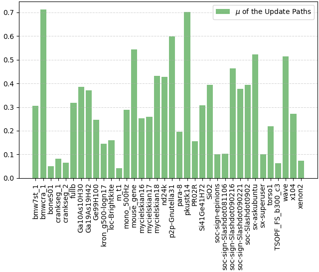
Figure 1. Evaluation of Weighted Version on 36 general graphs: Ratio of Updated Paths (Present the portion of $\mu$ that has increased)

On 36 general graphs, the weighted version of DAWN algorithm updated an average of 29.578% of the paths, with range of [4.279%, 71.118%]. These results indicate that the mean value of $\mu$ is equal to 1.296, which is dependent on the structure of the graphs, such that even changing the edge weights on the same graph can affect its value.

Experimental results have demonstrated that $\mu$ is a constant value independent of the number of nodes and edges in the graph. Furthermore, both the weighted version of DAWN and GDS algorithms exhibit similar time complexity on the general graphs. These findings provide a solid foundation for subsequent performance evaluations.

4.3. Scalability

4.4. Speedup

4.5. Latency

4.6. Large-scale Graph

5. Conclusion

In this paper, we propose a weighted version of DAWN, which requires $O(\mu\cdot n\cdot m)$ and $O(\mu\cdot S_{wcc}\cdot E_{wcc})$ time on the connected and unconnected graphs for APSP problems, respectively. The weighted version of DAWN requires $O(\mu\cdot m)$ and $O(\mu\cdot E_{wcc})$ time on the connected and unconnected graphs for SSSP problems.

The experimental results demonstrate that DAWN exhibits significant performance improvement on high-performance processors and surpasses Gunrock’s performance even on low-cost processors. DAWN demonstrates superior performance and broader applicability over GDS on large-scale graphs.

The high scalability and high parallelism of DAWN provide a solution for the analysis of the shortest paths problem in various graphs. We will develop the version of DAWN running on the weighted graph in the future. We hope to take the DAWN from a promising proof-of-concept to a practical tool that can be used for real-world graph analysis applications in the future.

- (1)
- Bellman (1958) Richard Bellman. 1958. On a routing problem. Quarterly of applied mathematics 16, 1 (1958), 87–90.
- Busato and Bombieri (2015) Federico Busato and Nicola Bombieri. 2015. An efficient implementation of the Bellman-Ford algorithm for Kepler GPU architectures. IEEE Transactions on Parallel and Distributed Systems 27, 8 (2015), 2222–2233.
- Cherkassky et al. (1996) Boris V Cherkassky, Andrew V Goldberg, and Tomasz Radzik. 1996. Shortest paths algorithms: Theory and experimental evaluation. Mathematical programming 73, 2 (1996), 129–174.
- Davidson et al. (2014) Andrew Davidson, Sean Baxter, Michael Garland, and John D Owens. 2014. Work-efficient parallel GPU methods for single-source shortest paths. In 2014 IEEE 28th International Parallel and Distributed Processing Symposium. IEEE, 349–359.
- Davis and Hu (2011) Timothy A. Davis and Yifan Hu. 2011. The University of Florida Sparse Matrix Collection. ACM Trans. Math. Softw. 38, 1 (dec 2011).
- Dijkstra et al. (1959) Edsger W Dijkstra et al. 1959. A note on two problems in connexion with graphs. Numerische mathematik 1, 1 (1959), 269–271.
- Djidjev et al. (2014) Hristo Djidjev, Sunil Thulasidasan, Guillaume Chapuis, Rumen Andonov, and Dominique Lavenier. 2014. Efficient multi-GPU computation of all-pairs shortest paths. In 2014 IEEE 28th International Parallel and Distributed Processing Symposium. IEEE, 360–369.
- Feng et al. (2023) Yelai Feng, Huaixi Wang, Yining Zhu, Chao Chang, and Hongyi Lu. 2023. A Novel Shortest Paths Algorithm on Unweighted Graphs. arXiv:2208.04514 [cs.DC]
- Floyd (1962) Robert W Floyd. 1962. Algorithm 97: shortest path. Commun. ACM 5, 6 (1962), 345.
- Johnson (1977) Donald B Johnson. 1977. Efficient algorithms for shortest paths in sparse networks. Journal of the ACM (JACM) 24, 1 (1977), 1–13.
- Leskovec and Krevl (2014) Jure Leskovec and Andrej Krevl. 2014. SNAP Datasets: Stanford Large Network Dataset Collection. http://snap.stanford.edu/data.
- Martín et al. (2009) Pedro J Martín, Roberto Torres, and Antonio Gavilanes. 2009. CUDA Solutions for the SSSP Problem. In International Conference on Computational Science. Springer, 904–913.
- Meyer and Sanders (2003) Ulrich Meyer and Peter Sanders. 2003. -stepping: a parallelizable shortest path algorithm. Journal of Algorithms 49, 1 (2003), 114–152.
- Ortega-Arranz et al. (2013) Hector Ortega-Arranz, Yuri Torres, Diego R Llanos, and Arturo Gonzalez-Escribano. 2013. A new GPU-based approach to the shortest path problem. In 2013 International Conference on High Performance Computing & Simulation (HPCS). IEEE, 505–511.
- Osama et al. (2022) Muhammad Osama, Serban D. Porumbescu, and John D. Owens. 2022. Essentials of Parallel Graph Analytics. In Proceedings of the Workshop on Graphs, Architectures, Programming, and Learning (GrAPL 2022). 314–317. https://doi.org/10.1109/IPDPSW55747.2022.00061
- Osama et al. (2023) Muhammad Osama, Serban D. Porumbescu, and John D. Owens. 2023. A Programming Model for GPU Load Balancing. In Proceedings of the 28th ACM SIGPLAN Annual Symposium on Principles and Practice of Parallel Programming (Montreal, QC, Canada) (PPoPP ’23). Association for Computing Machinery, New York, NY, USA, 79–91.
- Raman (1996) Rajeev Raman. 1996. Priority queues: Small, monotone and trans-dichotomous. In European Symposium on Algorithms. Springer, 121–137.
- Raman (1997) Rajeev Raman. 1997. Recent results on the single-source shortest paths problem. ACM SIGACT News 28, 2 (1997), 81–87.
- sao et al. (2021) piyush sao, Hao lu, Ramakrishnan Kannan, Vijay Thakkar, Richard Vuduc, and Thomas Potok. 2021. Scalable All-Pairs Shortest Paths for Huge Graphs on Multi-GPU Clusters. In Proceedings of the 30th International Symposium on High-Performance Parallel and Distributed Computing (Virtual Event, Sweden) (HPDC ’21). Association for Computing Machinery, New York, NY, USA, 121–131.
- Surve and Shah (2017) Ganesh G Surve and Medha A Shah. 2017. Parallel implementation of bellman-ford algorithm using CUDA architecture. In 2017 International conference of Electronics, Communication and Aerospace Technology (ICECA), Vol. 2. IEEE, 16–22.
- Thorup (1999) Mikkel Thorup. 1999. Undirected single-source shortest paths with positive integer weights in linear time. Journal of the ACM (JACM) 46, 3 (1999), 362–394.
- Thorup (2000) Mikkel Thorup. 2000. On RAM priority queues. SIAM J. Comput. 30, 1 (2000), 86–109.
- Wang et al. (2019) Hao Wang, Liang Geng, Rubao Lee, Kaixi Hou, Yanfeng Zhang, and Xiaodong Zhang. 2019. SEP-Graph: finding shortest execution paths for graph processing under a hybrid framework on GPU. In Proceedings of the 24th Symposium on Principles and Practice of Parallel Programming. 38–52.
- Wang et al. (2021) Kai Wang, Don Fussell, and Calvin Lin. 2021. A fast work-efficient SSSP algorithm for GPUs. In Proceedings of the 26th ACM SIGPLAN Symposium on Principles and Practice of Parallel Programming. 133–146.
- Wang et al. (2017) Yangzihao Wang, Yuechao Pan, Andrew Davidson, Yuduo Wu, Carl Yang, Leyuan Wang, Muhammad Osama, Chenshan Yuan, Weitang Liu, Andy T. Riffel, and John D. Owens. 2017. Gunrock: GPU Graph Analytics. ACM Transactions on Parallel Computing 4, 1 (Aug. 2017), 3:1–3:49.
- Yang et al. (2023) Shaofeng Yang, Xiandong Liu, Yunting Wang, Xin He, and Guangming Tan. 2023. Fast All-Pairs Shortest Paths Algorithm in Large Sparse Graph. In Proceedings of the 37th ACM International Conference on Supercomputing (Virtual Event) (ICS ’23). Association for Computing Machinery, Orlando, Florida, USA, Article 24, 13 pages.