False discovery proportion envelopes with consistency

Abstract

We provide new false discovery proportion (FDP) confidence envelopes in several multiple testing settings relevant for modern high dimensional-data methods. We revisit the scenarios considered in the recent work of Katsevich and Ramdas, (2020) (top-$k$, preordered — including knockoffs —, online) with a particular emphasis on obtaining FDP bounds that have both nonasymptotical coverage and asymptotical consistency, i.e. converge below the desired level $\alpha$ when applied to a classical $\alpha$-level false discovery rate (FDR) controlling procedure. This way, we derive new bounds that provide improvements over existing ones, both theoretically and practically, and are suitable for situations where at least a moderate number of rejections is expected. These improvements are illustrated with numerical experiments and real data examples. In particular, the improvement is significant in the knockoffs setting, which shows the impact of the method for a practical use. As side results, we introduce a new confidence envelope for the empirical cumulative distribution function of i.i.d. uniform variables and we provide new power results in sparse cases, both being of independent interest.

1 Introduction

1.1 Background

Multiple inference is a crucial issue in many modern, high dimensional, and massive data sets, for which a large number of variables are considered and many questions naturally emerge, either simultaneously or sequentially. Recent statistical inference has thus turned to designing methods that guard against false discoveries and selection effect, see Cui et al., (2021); Robertson et al., (2022) for recent reviews on that topic. A key quantity is typically the false discovery proportion (FDP), that is, the proportion of false discoveries within the selection (Benjamini and Hochberg,, 1995).

Among classical methods, finding confidence bounds on the FDP that are valid after a user data-driven selection ( ‘post hoc’ FDP bounds), has retained attention since the seminal works of Genovese and Wasserman, (2004, 2006); Goeman and Solari, (2011). The strategy followed by these works is to build confidence bounds valid uniformly over all selection subsets, which de facto provides a bound valid for any data-driven selection subset. A number of such FDP bounds have been proposed since, either based on a ‘closed testing’ paradigm (Hemerik et al.,, 2019; Goeman et al.,, 2019, 2021; Vesely et al.,, 2021), a ‘reference family’ (Blanchard et al.,, 2020; Durand et al.,, 2020), or a specific prior distribution in a Bayesian framework (Perrot-Dockès et al.,, 2021). It should also be noted that methods providing bounds valid uniformly over some particular selection subsets can also be used to provide bounds valid on any subsets by using an ‘interpolation’ technique, see, e.g., Blanchard et al., (2020). This is the case for instance for bounds based upon an empirical distribution function confidence band, as investigated by Meinshausen and Bühlmann, (2005); Meinshausen, (2006); Meinshausen and Rice, (2006); Dümbgen and Wellner, (2023). Loosely, we will refer to such (potentially partial) FDP bounds as FDP confidence envelopes in the sequel.

Recently, finding FDP confidence envelopes has been extended to different contexts of interest in Katsevich and Ramdas, (2020) (KR below for short), including knockoffs (Barber and Candès,, 2015; Candès et al.,, 2018) and online multiple testing (Aharoni and Rosset, 2014a, ). For this, their bounds are tailored on particular nested ‘paths’, and employ accurate martingale techniques. In addition, Li et al., (2022) have recently investigated specifically the case of the knockoffs setting by using a ‘joint’ $k$-FWER error rate control (see also Genovese and Wasserman,, 2006; Meinshausen,, 2006; Blanchard et al.,, 2020), possibly in combination with closed testing.

1.2 New insight: consistency

The main point of this paper is to look at FDP confidence envelopes towards the angle of a particular property that we call consistency. First recall that the false discovery rate (FDR) is the expectation of the FDP, which is a type I error rate measure with increasing popularity since the seminal work of Benjamini and Hochberg, (1995). Informally, an FDP confidence envelope is consistent, if its particular value on an FDR-controlling selection set is close to (or below) the corresponding nominal value, at least asymptotically. This property is important for several reasons:

• FDR controlling procedures are particular selection sets that are widely used in practice. Hence, it is very useful to provide an accurate FDP bound for these particular rejection sets. This is the case for instance for the commonly used Benjamini-Hochberg (BH) procedure at a level $\alpha$ — or even for a data dependent choice of the level $\hat{\alpha}$ — for which the FDP bound should be close to $\alpha$ (or $\hat{\alpha}$), at least in ‘favorable’ cases;

• a zoo of FDP confidence envelopes have been proposed in previous literature, and we see the consistency as a principled way to discard some of them while putting the emphasis on others;

• searching for consistency can also lead to new bounds that are accurate for a moderate sample size.

It turns out that most of the existing bounds, while being accurate in certain regimes, are not consistent. In particular, this is the case for those of Katsevich and Ramdas, (2020), because of a constant factor (larger than 1) in front of the FDP estimate. The present paper proposes to fill this gap by proposing new envelopes that are consistent. In a nutshell, we replace the constant in front of the FDP estimate by a function that tends to $1$ in a particular asymptotical regime.

Since we evoke consistency, it is worth emphasizing that the envelopes developed in this work have coverage holding in a non-asymptotical sense. Here, consistency means that on top of this strong non-asymptotical guarantee, the bound satisfies an additional sharpness condition in an asymptotical sense and for some scenarios of interest, including sparse ones.

1.3 Settings

Following Katsevich and Ramdas, (2020), we consider the three following multiple testing settings for which a ‘path’ means a (possibly random) nested sequence of candidate rejection sets:

• Top-$k$: the classical multiple testing setting where the user tests a finite number $m$ of null hypotheses and observes simultaneously a family of corresponding $p$-values. This is the framework of the seminal paper of Benjamini and Hochberg, (1995) and of the majority of the follow-up papers. In that case, the path is composed of the hypotheses corresponding to the top-$k$ most significant $p$-values (i.e. ranked in increasing order), for varying $k$.

• Pre-ordered: we observe $p$-values for a finite set of cardinal $m$ of null hypotheses, which are a priori arranged according to some ordering. In that setting, the signal (if any) is primarily carried by the ordering: alternatives are expected to be more likely to have a small rank. Correspondingly the path in that case is obtained by $p$-value thresholding (for fixed threshold) of the first $k$ hypotheses w.r.t. that order, for varying $k$. A typical instance is the knockoffs setting (Barber and Candès,, 2015; Candès et al.,, 2018), where the null hypotheses come from a high-dimensional linear regression model and one wants to test whether each of the $m$ variables is associated with the response. The ordering is data-dependent and comes from an ancillary statistic independent of the tests themselves, so that one can argue conditionally and consider the ordering (and path) as fixed.

• Online: the null hypotheses come sequentially, and there is a corresponding potentially infinite stream of $p$-values. An irrevocable decision (reject or not) has to be taken in turn for each new hypothesis, depending on past observations only. The path is naturally defined according to the set of rejections until time $t$, for varying $t$.

Let us introduce notation that encompasses the three settings mentioned above: the set of hypotheses is denoted by ${\mathcal{H}}$ (potentially infinite), the set of null hypotheses ${\mathcal{H}}_{0}$ is an unknown subset of ${\mathcal{H}}$, and a path $\Pi=(R_{k},k\geq 1)$ (with convention $R_{0}=\emptyset$) is an ordered sequence of nested subsets of ${\mathcal{H}}$ that depends only on the observations. A confidence envelope is a sequence $(\overline{\textnormal{FDP}}_{k},k\geq 1)$ (with convention $\overline{\textnormal{FDP}}_{0}=0$) of random variables valued in $[0,1]$, depending only on the observations, such that, for some pre-specified level $\delta$, we have

$$\mathbf{P}(\forall k\geq 1,\textnormal{FDP}(R_{k})\leq\overline{\textnormal{FDP}}_{k})\geq 1-\delta,$$ (1)

where $\textnormal{FDP}(R_{k})=\frac{|R_{k}\cap{\mathcal{H}}_{0}|}{|R_{k}|\vee 1}$ is the FDP of the set $R_{k}$. In (1), the guarantee is uniform in $k$, which means that it corresponds to confidence bounds valid uniformly over the subsets of the path. Also, distribution $\mathbf{P}$ is relative to the $p$-value model, which will be specified further on and depends on the considered framework.

Remark 1.1 (Interpolation).

On can notice here that any FDP confidence envelope of the type (1) can also lead to a post hoc FDP bound valid uniformly for all $R\subset{\mathcal{H}}$: specifically, by using the interpolation method (see, e.g., Blanchard et al.,, 2020; Goeman et al.,, 2021; Li et al.,, 2022), if (1) holds then the relation also holds with the sharper bound $({\widetilde{\textnormal{FDP}}}_{k},k\geq 1)$ given by

$${\widetilde{\textnormal{FDP}}}_{k} =\frac{\min_{k^{\prime}\leq k}\{|R_{k}\cap(R_{k^{\prime}})^{c}|+|R_{k^{\prime}}|\overline{\textnormal{FDP}}_{k^{\prime}}\}}{|R_{k}|\vee 1},$$ (2)

due to the fact that the number of false positives in $R_{k}$ is always bounded by the number of false positives in $R_{k^{\prime}}\subset R_{k}$ plus the number of elements of $R_{k}\cap(R_{k^{\prime}})^{c}$.

Particular subsets of $\Pi=(R_{k},k\geq 1)$ that are of interest are those controlling the FDR. Given a nominal level $\alpha$, a ‘reference’ procedure chooses a data-dependent $\hat{k}_{\alpha}$ such that $\mathbb{E}\IfEqCase{a}{{a}{\mathopen{}\mathclose{{}\left[\textnormal{FDP}(R_{\hat{k}_{\alpha}})}\right]}{0}{[\textnormal{FDP}(R_{\hat{k}_{\alpha}})]}{1}{\big{[}\textnormal{FDP}(R_{\hat{k}_{\alpha}})\big{]}}{2}{\Big{[}\textnormal{FDP}(R_{\hat{k}_{\alpha}})\Big{]}}{3}{\bigg{[}\textnormal{FDP}(R_{\hat{k}_{\alpha}})\bigg{]}}{4}{\Bigg{[}\textnormal{FDP}(R_{\hat{k}_{\alpha}})\Bigg{]}}}[]\leq\alpha$. Depending on the setting, we consider different reference procedures:

• Top-$k$ setting: the reference FDR controlling procedure is the Benjamini-Hochberg (BH) step-up procedure, see Benjamini and Hochberg, (1995);

• Pre-ordered setting: the reference procedure is the Lei-Fithian (LF) adaptive Selective sequential step-up procedure, see Lei and Fithian, (2016) (itself being a generalization of the procedure of Li and Barber,, 2017);

• Online setting: the reference procedure is the (LORD) procedure, see Javanmard and Montanari, (2018) and more precisely the improved version of Ramdas et al., (2017).

As announced, for all these procedures, the expectation of the FDP (that is, the FDR) is guaranteed to be below $\alpha$. On the other hand, it is commonly the case that in an appropriate asymptotic setting, the FDP concentrates around its expectation, see, e.g., Genovese and Wasserman, (2004); Neuvial, (2008, 2013). Therefore, an adequate confidence bound on the FDP should asymptotically converge to (or below) $\alpha$ when applied to a reference procedure. Furthermore, we emphasize once more that we aim at a bound which is valid non-asymptotically, and uniformly over the choice of $\alpha$ (or equivalently $k$) to account for possible ‘data snooping’ from the user (that is, $\alpha=\hat{\alpha}$ is possibly depending on the data).

Let us now make the definition of consistency more precise.

Definition 1.2 (Consistency for top-$k$ and pre-ordered settings).

Let $\delta\in(0,1)$ be fixed. For each $m\geq 1$, let $\mathbf{P}^{(m)}$ be a multiple testing model over the hypotheses set ${\mathcal{H}}=\{1,\dots,m\}$, $\Pi=(R_{k},k\geq 1)$ be a possibly random path of nested subsets of ${\mathcal{H}}$, and $(\overline{\textnormal{FDP}}_{k},k\geq 1)$ a confidence envelope at level $1-\delta$ over that path, i.e. satisfying (1) (for $\mathbf{P}=\mathbf{P}^{(m)}$). For any $\alpha\in(0,1)$, let ${\hat{k}_{\alpha}}$ be an FDR controlling procedure at level $\alpha$, i.e. satisfying $\mathbf{E}^{(m)}\IfEqCase{a}{{a}{\mathopen{}\mathclose{{}\left[\textnormal{FDP}(R_{\hat{k}_{\alpha}})}\right]}{0}{[\textnormal{FDP}(R_{\hat{k}_{\alpha}})]}{1}{\big{[}\textnormal{FDP}(R_{\hat{k}_{\alpha}})\big{]}}{2}{\Big{[}\textnormal{FDP}(R_{\hat{k}_{\alpha}})\Big{]}}{3}{\bigg{[}\textnormal{FDP}(R_{\hat{k}_{\alpha}})\bigg{]}}{4}{\Bigg{[}\textnormal{FDP}(R_{\hat{k}_{\alpha}})\Bigg{]}}}[]\leq\alpha$. Then the confidence envelope is said to be consistent for the sequence $(\mathbf{P}^{(m)},m\geq 1)$ and for the FDR controlling procedure $R_{\hat{k}_{\alpha}}\in\Pi$ at a level $\alpha$ in a range $[\alpha_{0},1)\subset(0,1)$, if for all $\epsilon>0$,

$$\lim_{m\rightarrow\infty}\mathbf{P}^{(m)}\mathopen{}\mathclose{{}\left(\sup_{\alpha\in[\alpha_{0},1)}\IfEqCase{a}{{a}{\mathopen{}\mathclose{{}\left\{\overline{\textnormal{FDP}}_{\hat{k}_{\alpha}}-\alpha}\right\}}{0}{\{\overline{\textnormal{FDP}}_{\hat{k}_{\alpha}}-\alpha\}}{1}{\big{\{}\overline{\textnormal{FDP}}_{\hat{k}_{\alpha}}-\alpha\big{\}}}{2}{\Big{\{}\overline{\textnormal{FDP}}_{\hat{k}_{\alpha}}-\alpha\Big{\}}}{3}{\bigg{\{}\overline{\textnormal{FDP}}_{\hat{k}_{\alpha}}-\alpha\bigg{\}}}{4}{\Bigg{\{}\overline{\textnormal{FDP}}_{\hat{k}_{\alpha}}-\alpha\Bigg{\}}}}[]\geq\epsilon}\right)=0.$$ (3)

In the above definition, $\mathbf{P}^{(m)}$ stands for a multiple testing model with $m$ hypotheses that is to be specified. We will be interested in standard model sequences that represent relevant practical situations, in particular sparse cases where a vanishing proportion of null hypotheses are false when $m$ tends to infinity. This definition applies for the two first considered settings (top-$k$ and pre-ordered). Note that due to (1), we have

$$\mathbf{P}(\forall\alpha\in(0,1),\textnormal{FDP}(R_{\hat{k}_{\alpha}})\leq\overline{\textnormal{FDP}}_{\hat{k}_{\alpha}})\geq 1-\delta.$$ (4)

Hence, (3) comes as an additional asymptotical accuracy guarantee to the non-asymptotical coverage property (4). Moreover, the uniformity in $\alpha$ in (4)-(3) allows for choosing $\alpha$ in a post hoc manner, while maintaining the false discovery control and without paying too much in accuracy, that is, for any data-dependent choice of $\hat{\alpha}$, $\textnormal{FDP}(R_{\hat{k}_{\hat{\alpha}}})\leq\overline{\textnormal{FDP}}_{\hat{k}_{\hat{\alpha}}}$ with probability at least $1-\delta$, with $\overline{\textnormal{FDP}}_{\hat{k}_{\hat{\alpha}}}\lesssim\hat{\alpha}(1+o(1))$ in ‘good’ cases.

In the third setting, an online FDR controlling procedure provides in itself a sequence $(R_{k},k\geq 1)$ and not a single set $R_{\hat{k}_{\alpha}}$. As a consequence, a confidence envelope $(\overline{\textnormal{FDP}}_{k},k\geq 1)$ is defined specifically for each procedure $(R_{k},k\geq 1)$. Hence, the definition should be slightly adapted:

Definition 1.3 (Consistency for online setting).

Let $\delta\in(0,1)$ be fixed and $\mathbf{P}$ be an online multiple testing model over the infinite hypothesis set ${\mathcal{H}}=\{1,2,\dots\}$. Let $(R_{k},k\geq 1)$ be an (online) FDR controlling procedure at level $\alpha$, i.e. such that $\sup_{k\geq 1}\mathbb{E}\IfEqCase{a}{{a}{\mathopen{}\mathclose{{}\left[\textnormal{FDP}(R_{k})}\right]}{0}{[\textnormal{FDP}(R_{k})]}{1}{\big{[}\textnormal{FDP}(R_{k})\big{]}}{2}{\Big{[}\textnormal{FDP}(R_{k})\Big{]}}{3}{\bigg{[}\textnormal{FDP}(R_{k})\bigg{]}}{4}{\Bigg{[}\textnormal{FDP}(R_{k})\Bigg{]}}}[]\leq\alpha$, and $(\overline{\textnormal{FDP}}_{k},k\geq 1)$ be a corresponding confidence envelope at level $1-\delta$, i.e., satisfying (1). Then $(\overline{\textnormal{FDP}}_{k},k\geq 1)$ is said to be consistent for the model $\mathbf{P}$ if for all $\epsilon>0$,

$$\lim_{k\to\infty}\mathbf{P}\mathopen{}\mathclose{{}\left(\overline{\textnormal{FDP}}_{k}-\alpha\geq\epsilon}\right)=0.$$ (5)

Note that both in (1) and (5) no uniformity w.r.t. the level $\alpha$ is imposed in the online setting.

1.4 Contributions

Our findings are as follows:

• In each of the considered settings (top-$k$, pre-ordered, online), we provide new (non-asymptotical) FDP confidence envelopes that are consistent under some mild conditions, including sparse configurations, see Proposition 2.5 (top-$k$), Proposition 3.4 (pre-ordered) and Proposition 4.5 (online). Table 1 provides a summary of the considered procedures in the different contexts, including the existing and new ones. It is worth noting that in the top-$k$ setting, the envelope based on the DKW inequality (Massart,, 1990) is consistent under moderate sparsity assumptions only, while the new envelope based on the Wellner inequality (Shorack and Wellner,, 2009) covers all the sparsity range (Proposition 2.5).

• As a byproduct, our results provide (non-asymptotical) confidence bounds on the FDP for standard FDR-controlling procedures which are asymptotically sharp (consistency) and for which a data-driven choice of the level $\alpha$ is allowed. In particular, in the top-$k$ setting, this gives a new sharp confidence bound for the achieved FDP of the BH procedure while tuning the level from the same data, see (18) below.

• In the top-$k$ setting, we also develop adaptive envelopes, for which the proportion of null hypotheses is simultaneously estimated, see Section 2.5. This is a novel approach with respect to existing literature and it is shown to improve significantly the bounds on simulations in ‘dense’ situations, see Section 5.

• In the pre-ordered setting, including the ‘knockoff’ case, we introduce new envelopes, called ‘Freedman’ and ‘KR-U’, which are the two first (provably-)consistent confidence bounds in that context to our knowledge. This is an important contribution since the knockoff method is one of the leading methodology in the literature of the last decade. In addition, KR-U is shown to behave suitably, even for moderate sample size, see Section 5.

• Our study is based on dedicated tools of independent interest, based on uniform versions of classical deviation inequalities, see Corollary 2.1 (Wellner’s inequality), Corollary C.5 (Freedman’s inequality). Both can be seen as a form of ‘stitching’ together elementary inequalities, see Howard et al., (2021) for recent developments of this principle. The bounds developed here are presented in a self-contained manner.

	Simes	DKW	KR	Wellner (new)	Freedman (new)	KR-U (new)
Top-$k$	No	Yes	No	Yes
Pre-ordered			No		Yes	Yes
Online			No		Yes	Yes

Table 1: Consistency property (Yes or No) for different envelopes, depending on the considered contexts. ‘Consistent’ means consistent at least in a particular (reasonable) configuration. Unfilled means undefined in that context.

2 Results in the top-$k$ case

2.1 Top-$k$ setting

We consider the classical multiple setting where we observe $m$ independent $p$-values $p_{1},\dots,p_{m}$, testing $m$ null hypotheses $H_{1},\dots,H_{m}$. The set of true nulls is denoted by ${\mathcal{H}}_{0}$, which is of cardinal $m_{0}$ and we denote $\pi_{0}=m_{0}/m\in(0,1)$. We assume that the $p$-values are uniformly distributed under the null, that is, for all $i\in{\mathcal{H}}_{0}$, $p_{i}\sim U(0,1)$.

We consider here the task of building a $(1-\delta)$-confidence envelope (1) for the top-$k$ path

$$R_{k}=\{1\leq i\leq m\>:\>p_{i}\leq p_{(k)}\},\>\>\>k=1,\dots,m.$$ (6)

A rejection set of particular interest is the BH rejection set, given by $R_{\hat{k}_{\alpha}}$ where

$$\hat{k}_{\alpha}=\max\mathopen{}\mathclose{{}\left\{k\in\mathbb{N}\>:\>{\widehat{\textnormal{FDP}}}_{k}\leq\alpha}\right\},\>\>{\widehat{\textnormal{FDP}}}_{k}=mp_{k}/k,$$ (7)

(with the convention $R_{0}=\emptyset$).

2.2 Existing envelopes

Let us first review the prominent confidence envelopes that have been considered in the literature. Let $U_{1},\dots,U_{n}$ be $n\geq 1$ i.i.d. uniform random variables. For $\delta\in(0,1)$, each of the following (uniform) inequalities holds with probability at least $1-\delta$:

• Simes (or Robbins,, 1954): for all $t\in(0,1)$, $n^{-1}\sum_{i=1}^{n}{\bm{1}\IfEqCase{a}{{a}{\mathopen{}\mathclose{{}\left\{U_{i}\leq t}\right\}}{0}{\{U_{i}\leq t\}}{1}{\big{\{}U_{i}\leq t\big{\}}}{2}{\Big{\{}U_{i}\leq t\Big{\}}}{3}{\bigg{\{}U_{i}\leq t\bigg{\}}}{4}{\Bigg{\{}U_{i}\leq t\Bigg{\}}}}[]}\leq t/\delta.$

• DKW (Massart,, 1990): for all $t\in(0,1)$, $n^{-1}\sum_{i=1}^{n}{\bm{1}\IfEqCase{a}{{a}{\mathopen{}\mathclose{{}\left\{U_{i}\leq t}\right\}}{0}{\{U_{i}\leq t\}}{1}{\big{\{}U_{i}\leq t\big{\}}}{2}{\Big{\{}U_{i}\leq t\Big{\}}}{3}{\bigg{\{}U_{i}\leq t\bigg{\}}}{4}{\Bigg{\{}U_{i}\leq t\Bigg{\}}}}[]}\leq t+\sqrt{\log(1/\delta)/2}\>n^{-1/2}.$

• KR (Katsevich and Ramdas,, 2020) (for $\delta\leq 0.31$), for all $t\in(0,1)$, $n^{-1}\sum_{i=1}^{n}{\bm{1}\IfEqCase{a}{{a}{\mathopen{}\mathclose{{}\left\{U_{i}\leq t}\right\}}{0}{\{U_{i}\leq t\}}{1}{\big{\{}U_{i}\leq t\big{\}}}{2}{\Big{\{}U_{i}\leq t\Big{\}}}{3}{\bigg{\{}U_{i}\leq t\bigg{\}}}{4}{\Bigg{\{}U_{i}\leq t\Bigg{\}}}}[]}\leq\frac{\log(1/\delta)}{\log(1+\log(1/\delta))}(1/n+t).$

Taking $(U_{1},\dots,U_{n})=(p_{i},i\in{\mathcal{H}}_{0})$, $n=m_{0}$, and $t=p_{(k)}$ in the bounds above gives the following confidence envelopes (in the sense of (1)) for the top-$k$ path: for $k\in\{1,\dots,m\}$,

$$\overline{\textnormal{FDP}}^{{\tiny\mbox{Simes}}}_{k} =1\wedge\frac{mp_{(k)}}{k\delta};$$ (8)

$$\overline{\textnormal{FDP}}^{{\tiny\mbox{DKW}}}_{k} =1\wedge\mathopen{}\mathclose{{}\left(\frac{mp_{(k)}}{k}+\frac{m^{1/2}\sqrt{0.5\log 1/\delta}}{k}}\right);$$ (9)

$$\overline{\textnormal{FDP}}^{{\tiny\mbox{KR}}}_{k} =1\wedge\mathopen{}\mathclose{{}\left(\frac{\log(1/\delta)}{\log(1+\log(1/\delta))}\mathopen{}\mathclose{{}\left(\frac{mp_{(k)}}{k}+1/k}\right)}\right),$$ (10)

the last inequality requiring in addition $\delta\leq 0.31$. Please note that we can slightly improve these bounds by taking appropriate integer parts, but we will ignore this detail further on for the sake of simplicity.

2.3 New envelope

In addition to the above envelopes, this section presents a new one deduced from a new ‘uniform’ variation of Wellner’s inequality (recalled in Lemma D.2). Let us first define the function

$$h(\lambda)=\lambda(\log\lambda-1)+1,\>\>\>\lambda>1.$$ (11)

Lemma D.1 gathers some properties of $h$, including explicit accurate bounds for $h$ and $h^{-1}$.

Proposition 2.1 (Uniform version of Wellner’s inequality).

Let $U_{1},\dots,U_{n}$ be $n\geq 1$ i.i.d. uniform random variables and $\kappa=\pi^{2}/6$. For all $\delta\in(0,1)$, we have with probability at least $1-\delta$,

$$\forall t\in(0,1),\>\>n^{-1}\sum_{i=1}^{n}{\bm{1}\IfEqCase{a}{{a}{\mathopen{}\mathclose{{}\left\{U_{i}\leq t}\right\}}{0}{\{U_{i}\leq t\}}{1}{\big{\{}U_{i}\leq t\big{\}}}{2}{\Big{\{}U_{i}\leq t\Big{\}}}{3}{\bigg{\{}U_{i}\leq t\bigg{\}}}{4}{\Bigg{\{}U_{i}\leq t\Bigg{\}}}}[]}\leq t\>h^{-1}\mathopen{}\mathclose{{}\left(\frac{\log(\kappa/\delta)+2\log\mathopen{}\mathclose{{}\left(\lceil\log_{2}(1/t)\rceil}\right)}{ng(t)}}\right),$$ (12)

for $g(t)=2^{-\lceil\log_{2}(1/t)\rceil}/(1-2^{-\lceil\log_{2}(1/t)\rceil})\geq t/2$ and $h(\cdot)$ defined by (11). In particular, with probability at least $1-\delta$,

$$\forall t\in(0,1),\>\>n^{-1}\sum_{i=1}^{n}{\bm{1}\IfEqCase{a}{{a}{\mathopen{}\mathclose{{}\left\{U_{i}\leq t}\right\}}{0}{\{U_{i}\leq t\}}{1}{\big{\{}U_{i}\leq t\big{\}}}{2}{\Big{\{}U_{i}\leq t\Big{\}}}{3}{\bigg{\{}U_{i}\leq t\bigg{\}}}{4}{\Bigg{\{}U_{i}\leq t\Bigg{\}}}}[]}\leq t\>h^{-1}\mathopen{}\mathclose{{}\left(\frac{2\log(\kappa/\delta)+4\log\mathopen{}\mathclose{{}\left(1+\log_{2}(1/t)}\right)}{nt}}\right).$$ (13)

The proof of Proposition 2.1 is given in Section B.1. It immediately leads to the following result.

Theorem 2.2.

In the top-$k$ setting of Section 2.1, the following quantity is a $(1-\delta)$-confidence envelope in the sense of (1) for the top-$k$ path:

$$\overline{\textnormal{FDP}}_{k}^{{\tiny\mbox{Well}}}=1\wedge\mathopen{}\mathclose{{}\left(\frac{mp_{(k)}}{k}\>h^{-1}\mathopen{}\mathclose{{}\left(\frac{2\log(\kappa/\delta)+4\log\mathopen{}\mathclose{{}\left(1+\log_{2}(1/p_{(k)})}\right)}{mp_{(k)}}}\right)}\right),$$ (14)

with $\kappa=\pi^{2}/6$.

Proof.

We use (13) for $(U_{1},\dots,U_{n})=(p_{i},i\in{\mathcal{H}}_{0})$, $n=m_{0}$, and $t=p_{(k)}$. We conclude by using $m_{0}\leq m$ and the monotonicity property of Lemma D.1. ∎

Remark 2.3.

Denoting by $\overline{F}_{n}(t)$ the RHS of (13), we can easily check

$$\sup_{t\in((\log\log n)/n,1)}\mathopen{}\mathclose{{}\left(\sqrt{n}\frac{\overline{F}_{n}(t)-t}{\sqrt{t\log\mathopen{}\mathclose{{}\left(1+\log_{2}(1/t)}\right)}}}\right) =O(1),$$

with a constant possibly depending on $\delta$. The iterated logarithm in the denominator is known from classical asymptotic theory (convergence to a Brownian bridge) to be unimprovable for a uniform bound in the vicinity of $0$; in this sense the above is a ‘finite law of the iterated logarithm (LIL) bound’ (Jamieson et al.,, 2014).

2.4 FDP confidence bounds for BH and consistency

Applying the previous bounds for the particular BH rejection sets $R_{\hat{k}_{\alpha}}$ (see (7)) leads to the following result.

Corollary 2.4.

In the top-$k$ setting of Section 2.1, for any $\alpha,\delta\in(0,1)$, the following quantities are $(1-\delta)$-confidence bounds for $\textnormal{FDP}(R_{\hat{k}_{\alpha}})$, the FDP of the BH procedure at level $\alpha$:

$$\overline{\textnormal{FDP}}^{{\tiny\mbox{Simes}}}_{\alpha} =1\wedge(\alpha/\delta);$$ (15)

$$\overline{\textnormal{FDP}}^{{\tiny\mbox{DKW}}}_{\alpha} =1\wedge\mathopen{}\mathclose{{}\left(\alpha+\frac{m^{1/2}\sqrt{0.5\log 1/\delta}}{1\vee\hat{k}_{\alpha}}}\right);$$ (16)

$$\overline{\textnormal{FDP}}^{{\tiny\mbox{KR}}}_{\alpha} =1\wedge\mathopen{}\mathclose{{}\left(\frac{\log(1/\delta)}{\log(1+\log(1/\delta))}\mathopen{}\mathclose{{}\left(\alpha+1/(1\vee\hat{k}_{\alpha})}\right)}\right);$$ (17)

$$\overline{\textnormal{FDP}}_{\alpha}^{{\tiny\mbox{Well}}} =1\wedge\mathopen{}\mathclose{{}\left(\alpha\>h^{-1}\mathopen{}\mathclose{{}\left(\frac{2\log(\kappa/\delta)+4\log\mathopen{}\mathclose{{}\left(1+\log_{2}\Big{(}\frac{m}{\alpha(1\vee\hat{k}_{\alpha})}\Big{)}}\right)}{\alpha(1\vee\hat{k}_{\alpha})}}\right)}\right),$$ (18)

where $\kappa=\pi^{2}/6$, $\hat{k}_{\alpha}$ denotes the number of rejections of the BH procedure (7) at level $\alpha$, and where the KR bound requires in addition $\delta\leq 0.31$. Moreover, these bounds are also valid uniformly in $\alpha\in(0,1)$, in the sense that

$$\mathbf{P}(\forall\alpha\in(0,1),\textnormal{FDP}(R_{\hat{k}_{\alpha}})\leq\overline{\textnormal{FDP}}_{\alpha}^{{\tiny\mbox{Meth}}})\geq 1-\delta,\>\>\mbox{Meth}\in\{{\mbox{Simes}},{\mbox{DKW}},{\mbox{KR}},{\mbox{Well}}\},$$

and thus also when using a post hoc choice $\alpha=\hat{\alpha}$ of the level.

Proof.

For (18), we use (13) for $(U_{1},\dots,U_{n})=(p_{i},i\in{\mathcal{H}}_{0})$, $n=m_{0}$, and $t=\alpha(1\vee\hat{k}_{\alpha})/m$. ∎

Let us now consider the consistency property (3). Among the four above bounds, it is apparent that Simes and KR are never consistent, because of the constant in front of $\alpha$; namely, for all $m$,

$$\overline{\textnormal{FDP}}^{{\tiny\mbox{Simes}}}_{\alpha}\wedge\overline{\textnormal{FDP}}^{{\tiny\mbox{KR}}}_{\alpha}\geq 1\wedge(c\alpha),$$

for some constant $c>1$. By contrast, $\overline{\textnormal{FDP}}_{\alpha}^{{\tiny\mbox{DKW}}}$ and $\overline{\textnormal{FDP}}_{\alpha}^{{\tiny\mbox{Well}}}$ are consistent in the sense of (3) in a regime such that $m^{1/2}/\hat{k}_{\alpha_{0}}=o_{P}(1)$ and $(\log\log m)/\hat{k}_{\alpha_{0}}=o_{P}(1)$, respectively. The latter means that the BH procedure at level $\alpha_{0}$ should make enough rejections. This is discussed for a particular setting in the next result.

Proposition 2.5.

Let us consider the sequence of sparse one-sided Gaussian location models $(\mathbf{P}^{(m)}_{b,c,\beta},m\geq 1)$ with fixed parameters $b\in\mathbb{R}$, $c\in(0,1)$ and a sparsity parameter $\beta\in[0,1)$, as defined in Section A.1. Then we have for all $\alpha\in(0,1)$,

$$\overline{\textnormal{FDP}}_{\alpha}^{{\tiny\mbox{DKW}}}-\alpha \asymp_{\mathbf{P}^{(m)}_{b,c,\beta}}m^{-1/2+\beta};$$

$$\overline{\textnormal{FDP}}_{\alpha}^{{\tiny\mbox{Well}}}-\alpha \asymp_{\mathbf{P}^{(m)}_{b,c,\beta}}\sqrt{\log\log(m)}\>m^{-1/2+\beta/2},$$

where $u_{m}\asymp_{P}v_{m}$ stands for $u_{m}=O_{P}(v_{m})$ and $v_{m}=O_{P}(u_{m})$. In particular, concerning the consistency (3) for the sequence $(\mathbf{P}^{(m)}_{b,c,\beta},m\geq 1)$ and the BH procedure:

• for the DKW envelope (9) and the corresponding bound (16), the consistency (3) holds when $\beta<1/2$ but fails for $\beta\geq 1/2$;

• for the Wellner envelope (14) and the corresponding bound (18), the consistency (3) holds for any arbitrary $\beta\in(0,1)$.

Proof.

By Theorem A.2, we have $\hat{k}_{\alpha}\asymp_{\mathbf{P}^{(m)}_{b,c,\beta}}m^{1-\beta}$. This gives the result (by applying in addition Lemma D.1 for the Wellner bound). ∎

Proposition 2.5 shows the superiority of the Wellner bound on the DKW bound for achieving the consistency property on a particular sparse sequence models: while the DKW bound needs a model dense enough ($\beta<1/2$), the Wellner bound covers the whole sparsity range $\beta\in(0,1)$.

2.5 Adaptive envelopes

Let us consider the following upper-bounds for $m_{0}$:

$$\hat{m}_{0}^{{\tiny\mbox{Simes}}} =m\wedge\inf_{t\in(0,\delta)}\frac{V_{t}}{1-t/\delta};$$ (19)

$$\hat{m}_{0}^{{\tiny\mbox{DKW}}} =m\wedge\inf_{t\in(0,1)}\mathopen{}\mathclose{{}\left(\frac{C^{1/2}}{2(1-t)}+\sqrt{\frac{C}{4(1-t)^{2}}+\frac{V_{t}}{1-t}}}\right)^{2};$$ (20)

$$\hat{m}_{0}^{{\tiny\mbox{KR}}} =m\wedge\inf_{t\in(0,1/C^{\prime})}\frac{C^{\prime}+V_{t}}{1-C^{\prime}t};$$ (21)

$$\hat{m}_{0}^{{\tiny\mbox{Well}}} =m\wedge\inf_{t\in(0,1)}\mathopen{}\mathclose{{}\left(\sqrt{\frac{tC_{t}}{2(1-t)^{2}}}+\sqrt{\frac{C_{t}}{{2(1-t)^{2}}}+\frac{V_{t}}{1-t}}}\right)^{2},$$ (22)

where $V_{t}=\sum_{i=1}^{m}{\bm{1}\IfEqCase{a}{{a}{\mathopen{}\mathclose{{}\left\{p_{i}>t}\right\}}{0}{\{p_{i}>t\}}{1}{\big{\{}p_{i}>t\big{\}}}{2}{\Big{\{}p_{i}>t\Big{\}}}{3}{\bigg{\{}p_{i}>t\bigg{\}}}{4}{\Bigg{\{}p_{i}>t\Bigg{\}}}}[]}$, $C=\log(1/\delta)/2$, $C^{\prime}=\frac{\log(1/\delta)}{\log(1+\log(1/\delta))}$, $C_{t}=2\log(\kappa/\delta)+4\log\mathopen{}\mathclose{{}\left(1+\log_{2}(1/t)}\right)$, $\kappa=\pi^{2}/6$. Since $V_{t}/(1-t)$ corresponds to the so-called Storey estimator Storey, (2002), these four estimators can all be seen as Storey-type confidence bounds, each including a specific deviation term that takes into account the probability error $\delta$. Note that $\hat{m}_{0}^{{\tiny\mbox{DKW}}}$ was already proposed in Durand et al., (2020).

Proposition 2.6.

In the top-$k$ setting of Section 2.1, the envelopes defined by (8), (9), (10) and (14) with $m$ replaced by the corresponding bound $\hat{m}_{0}^{{\tiny\mbox{Simes}}}$ (19), $\hat{m}_{0}^{{\tiny\mbox{DKW}}}$ (20), $\hat{m}_{0}^{{\tiny\mbox{KR}}}$ (21) or $\hat{m}_{0}^{{\tiny\mbox{Well}}}$ (22), respectively, are also $(1-\delta)$-confidence envelopes in the sense of (1) for the top-$k$ path.

We can easily check that these four adaptive envelopes all uniformly improve their own non-adaptive counterpart. The proof of Proposition 2.6 is provided in Section B.2.

Remark 2.7.

In practice, the bounds $\hat{m}_{0}^{{\tiny\mbox{Simes}}}$ (19), $\hat{m}_{0}^{{\tiny\mbox{DKW}}}$ (20), $\hat{m}_{0}^{{\tiny\mbox{KR}}}$ (21) or $\hat{m}_{0}^{{\tiny\mbox{Well}}}$ (22) can be computed by taking an infimum over $t=p_{(k)}$, $1\leq k\leq m$ and by replacing $V_{t}$ by $m-k$.

Applying Proposition 2.6 for the BH procedure, this gives rise to the following adaptive confidence bounds.

Corollary 2.8.

In the top-$k$ setting of Section 2.1, for any $\alpha,\delta\in(0,1)$, the following quantities are $(1-\delta)$-confidence bounds for the FDP of the BH procedure at level $\alpha$:

$$\overline{\textnormal{FDP}}^{{\tiny\mbox{Simes-adapt}}}_{\alpha} =1\wedge\alpha(\hat{m}_{0}^{{\tiny\mbox{Simes}}}/{m})/\delta;$$ (23)

$$\overline{\textnormal{FDP}}^{{\tiny\mbox{DKW-adapt}}}_{\alpha} =1\wedge\Big{(}\alpha(\hat{m}_{0}^{{\tiny\mbox{DKW}}}/{m})+\frac{(\hat{m}_{0}^{{\tiny\mbox{DKW}}})^{1/2}\sqrt{0.5\log 1/\delta}}{1\vee\hat{k}_{\alpha}}\Big{)};$$ (24)

$$\overline{\textnormal{FDP}}^{{\tiny\mbox{KR-adapt}}}_{\alpha} =1\wedge\mathopen{}\mathclose{{}\left(\frac{\log(1/\delta)}{\log(1+\log(1/\delta))}\mathopen{}\mathclose{{}\left(\alpha(\hat{m}_{0}^{{\tiny\mbox{KR}}}/{m})+1/(1\vee\hat{k}_{\alpha})}\right)}\right);$$ (25)

$$\overline{\textnormal{FDP}}_{\alpha}^{{\tiny\mbox{Well-adapt}}} =1\wedge\mathopen{}\mathclose{{}\left(\alpha(\hat{m}_{0}^{{\tiny\mbox{Well}}}/{m})\>h^{-1}\mathopen{}\mathclose{{}\left(\frac{2\log(\kappa/\delta)+4\log\mathopen{}\mathclose{{}\left(1+\log_{2}\Big{(}\frac{m}{\alpha(1\vee\hat{k}_{\alpha})}\Big{)}}\right)}{\alpha(1\vee\hat{k}_{\alpha})\hat{m}_{0}^{{\tiny\mbox{Well}}}/{m}}}\right)}\right),$$ (26)

where $\kappa=\pi^{2}/6$, $\hat{k}_{\alpha}$ denotes the number of rejections of BH procedure (7) at level $\alpha$, and where the KR-adapt bound requires in addition $\delta\leq 0.31$. Moreover, these bounds are also valid uniformly in $\alpha\in(0,1)$ and thus also when using a post hoc choice $\alpha=\hat{\alpha}$ of the level.

Proof.

For (26), we use (13) for $(U_{1},\dots,U_{n})=(p_{i},i\in{\mathcal{H}}_{0})$, $n=m_{0}$, $t=\alpha(1\vee\hat{k}_{\alpha})/m$, and the fact that $m_{0}\leq\hat{m}_{0}^{{\tiny\mbox{Well}}}$ on the considered event by the proof in Section B.2. The other bounds are proved similarly. ∎

2.6 Interpolated bounds

According to Remark 1.1, the coverage (1) is still valid after the interpolation operation given by (2). As a result, the above confidence envelopes can be improved as follows:

$${\widetilde{\textnormal{FDP}}}^{{\tiny\mbox{Simes}}}_{k} =\min_{k^{\prime}\leq k}\{k-k^{\prime}+k^{\prime}\wedge(mp_{(k^{\prime})}/\delta)\}/k;$$ (27)

$${\widetilde{\textnormal{FDP}}}^{{\tiny\mbox{DKW}}}_{k} =\min_{k^{\prime}\leq k}\{k-k^{\prime}+k^{\prime}\wedge(mp_{(k^{\prime})}+m^{1/2}\sqrt{0.5\log 1/\delta})\}/k;$$ (28)

$${\widetilde{\textnormal{FDP}}}^{{\tiny\mbox{KR}}}_{k} =\min_{k^{\prime}\leq k}\mathopen{}\mathclose{{}\left\{k-k^{\prime}+k^{\prime}\wedge\mathopen{}\mathclose{{}\left(\frac{\log(1/\delta)}{\log(1+\log(1/\delta))}\mathopen{}\mathclose{{}\left(mp_{(k^{\prime})}+1}\right)}\right)}\right\}/k;$$ (29)

$${\widetilde{\textnormal{FDP}}}_{k}^{{\tiny\mbox{Well}}} =\min_{k^{\prime}\leq k}\mathopen{}\mathclose{{}\left\{k-k^{\prime}+k^{\prime}\wedge\mathopen{}\mathclose{{}\left(mp_{(k^{\prime})}\>h^{-1}\mathopen{}\mathclose{{}\left(\frac{2\log(\kappa/\delta)+4\log\mathopen{}\mathclose{{}\left(1+\log_{2}(1/p_{(k^{\prime})})}\right)}{mp_{(k^{\prime})}}}\right)}\right)}\right\}/k,$$ (30)

respectively. When applied to BH rejection set, this also provides new confidence bounds ${\widetilde{\textnormal{FDP}}}^{{\tiny\mbox{Simes}}}_{\alpha}$, ${\widetilde{\textnormal{FDP}}}^{{\tiny\mbox{DKW}}}_{\alpha}$, ${\widetilde{\textnormal{FDP}}}^{{\tiny\mbox{KR}}}_{\alpha}$, ${\widetilde{\textnormal{FDP}}}_{\alpha}^{{\tiny\mbox{Well}}}$, that can further be improved by replacing $m$ by the corresponding estimator $\hat{m}_{0}$.

3 Results in the pre-ordered case

In this section, we build consistent envelopes in the case where the $p$-values are ordered a priori, which covers the famous ‘knockoff’ case.

3.1 Pre-ordered setting

Let $\pi:\{1,\dots,m\}\to\{1,\dots,m\}$ be some ordering of the $p$-values that is considered as given and deterministic (possibly coming from independent data). The pre-ordered setting is formally the same as the one of Section 2.1, except that the $p$-value set is explored according to $\pi(1),\pi(2),\dots,\pi(m)$. The rationale behind this is that the alternative null hypotheses ${\mathcal{H}}_{1}=\{1,\dots,m\}\backslash{\mathcal{H}}_{0}$ are implicitly expected to be more likely to have a small rank in the ordering $\pi$ (although this condition is not needed for the future controlling results to hold).

Formally, the considered path is

$$R_{k}=\{\pi(i)\>:\>1\leq i\leq k,\>\>p_{\pi(i)}\leq s\},\>\>\>k=1,\dots,m,$$ (31)

for some fixed additional threshold $s\in(0,1]$ (possibly coming from independent data) and can serve to make a selection. The aim is still to find envelopes $(\overline{\textnormal{FDP}}_{k})_{k}$ satisfying (1) for this path while being consistent. To set up properly the consistency, we should consider an FDR controlling procedure that is suitable in this setting. For this, we consider the Lei Fithian (LF) adaptive Selective sequential step-up procedure (Lei and Fithian,, 2016). The latter is defined by $R_{\hat{k}_{\alpha}}$ where

$$\hat{k}_{\alpha}=\max\mathopen{}\mathclose{{}\left\{k\in\{0,\dots,m\}:{\widehat{\textnormal{FDP}}}_{k}\leq\alpha}\right\},\>\>{\widehat{\textnormal{FDP}}}_{k}=\frac{s}{1-\lambda}\frac{1+\sum_{i=1}^{k}{\bm{1}\IfEqCase{a}{{a}{\mathopen{}\mathclose{{}\left\{p_{\pi(i)}>\lambda}\right\}}{0}{\{p_{\pi(i)}>\lambda\}}{1}{\big{\{}p_{\pi(i)}>\lambda\big{\}}}{2}{\Big{\{}p_{\pi(i)}>\lambda\Big{\}}}{3}{\bigg{\{}p_{\pi(i)}>\lambda\bigg{\}}}{4}{\Bigg{\{}p_{\pi(i)}>\lambda\Bigg{\}}}}[]}}{1\vee\sum_{i=1}^{k}{\bm{1}\IfEqCase{a}{{a}{\mathopen{}\mathclose{{}\left\{p_{\pi(i)}\leq s}\right\}}{0}{\{p_{\pi(i)}\leq s\}}{1}{\big{\{}p_{\pi(i)}\leq s\big{\}}}{2}{\Big{\{}p_{\pi(i)}\leq s\Big{\}}}{3}{\bigg{\{}p_{\pi(i)}\leq s\bigg{\}}}{4}{\Bigg{\{}p_{\pi(i)}\leq s\Bigg{\}}}}[]}},$$ (32)

where $\lambda\in[0,1)$ is an additional parameter. The ‘knockoff’ setting of Barber and Candès, (2015) can be seen as a particular case of this pre-ordered setting, where the $p$-values are independent and binary, the ordering is independent of the $p$-values and $s=\lambda=1/2$. The LF procedure reduces in that case to the classical Barber and Candès (BC) procedure.

3.2 New confidence envelopes

The first envelope is as follows.

Theorem 3.1.

Consider the pre-ordered setting of Section 3.1 with $s\in(0,1]$. For all $\delta\in(0,1)$, $\lambda\in[0,1)$, the following is a $(1-\delta)$-confidence envelope for the ordered path (31) in the sense of (1):

$$\overline{\textnormal{FDP}}_{k}^{{\tiny\mbox{Freed}}}=1\wedge\frac{\frac{s}{1-\lambda}\sum_{i=1}^{k}{\bm{1}\IfEqCase{a}{{a}{\mathopen{}\mathclose{{}\left\{p_{\pi(i)}>\lambda}\right\}}{0}{\{p_{\pi(i)}>\lambda\}}{1}{\big{\{}p_{\pi(i)}>\lambda\big{\}}}{2}{\Big{\{}p_{\pi(i)}>\lambda\Big{\}}}{3}{\bigg{\{}p_{\pi(i)}>\lambda\bigg{\}}}{4}{\Bigg{\{}p_{\pi(i)}>\lambda\Bigg{\}}}}[]}+\Delta(\nu k)}{\sum_{i=1}^{k}{\bm{1}\IfEqCase{a}{{a}{\mathopen{}\mathclose{{}\left\{p_{\pi(i)}\leq s}\right\}}{0}{\{p_{\pi(i)}\leq s\}}{1}{\big{\{}p_{\pi(i)}\leq s\big{\}}}{2}{\Big{\{}p_{\pi(i)}\leq s\Big{\}}}{3}{\bigg{\{}p_{\pi(i)}\leq s\bigg{\}}}{4}{\Bigg{\{}p_{\pi(i)}\leq s\Bigg{\}}}}[]}},\>k\geq 1,$$ (33)

where $\Delta(u)=2\sqrt{\varepsilon_{u}}\sqrt{{(u\vee 1)}}+{\frac{1}{2}}\varepsilon_{u}$, $\varepsilon_{u}=\log((1+\kappa)/\delta)+2\log\mathopen{}\mathclose{{}\left(1+\log_{2}\mathopen{}\mathclose{{}\left(u\vee 1}\right)}\right)$, $u>0$, $\kappa=\pi^{2}/6$ and $\nu=s(1+\min(s,\lambda)/(1-\lambda))$.

The proof of Theorem 3.1 is a direct consequence of a more general result (Theorem C.1), itself being a consequence of a uniform version of Freedman’s inequality (see Section C.2).

The second result comes from the KR envelope (Katsevich and Ramdas,, 2020):

$$\overline{\textnormal{FDP}}^{\mbox{\tiny KR}}_{k}=1\wedge\mathopen{}\mathclose{{}\left(\frac{\log(1/\delta)}{a\log(1+\frac{1-\delta^{B/a}}{B})}\frac{a+\frac{s}{1-\lambda}\sum_{i=1}^{k}{\bm{1}\IfEqCase{a}{{a}{\mathopen{}\mathclose{{}\left\{p_{\pi(i)}>\lambda}\right\}}{0}{\{p_{\pi(i)}>\lambda\}}{1}{\big{\{}p_{\pi(i)}>\lambda\big{\}}}{2}{\Big{\{}p_{\pi(i)}>\lambda\Big{\}}}{3}{\bigg{\{}p_{\pi(i)}>\lambda\bigg{\}}}{4}{\Bigg{\{}p_{\pi(i)}>\lambda\Bigg{\}}}}[]}}{1\vee\sum_{i=1}^{k}{\bm{1}\IfEqCase{a}{{a}{\mathopen{}\mathclose{{}\left\{p_{\pi(i)}\leq s}\right\}}{0}{\{p_{\pi(i)}\leq s\}}{1}{\big{\{}p_{\pi(i)}\leq s\big{\}}}{2}{\Big{\{}p_{\pi(i)}\leq s\Big{\}}}{3}{\bigg{\{}p_{\pi(i)}\leq s\bigg{\}}}{4}{\Bigg{\{}p_{\pi(i)}\leq s\Bigg{\}}}}[]}}}\right),$$ (34)

where $a>0$ is some parameter, $B=s/(1-\lambda)$ and it is assumed $\lambda\geq s$. While the default choice in KR is $a=1$, we can build up a new envelope by taking a union bound over $a\in\mathbb{N}\backslash\{0\}$:

Theorem 3.2.

Consider the pre-ordered setting of Section 3.1 with $s\in(0,1]$. For all $\delta\in(0,1)$ and $\lambda\in[s,1]$, the following is a $(1-\delta)$-confidence envelope for the ordered path (31) in the sense of (1):

$$\overline{\textnormal{FDP}}_{k}^{{\tiny\mbox{KR-U}}}=1\wedge\min_{a\in\mathbb{N}\backslash\{0\}}\mathopen{}\mathclose{{}\left\{\frac{\log(1/\delta_{a})}{a\log(1+\frac{1-\delta_{a}^{B/a}}{B})}\frac{a+\frac{s}{1-\lambda}\sum_{i=1}^{k}{\bm{1}\IfEqCase{a}{{a}{\mathopen{}\mathclose{{}\left\{p_{\pi(i)}>\lambda}\right\}}{0}{\{p_{\pi(i)}>\lambda\}}{1}{\big{\{}p_{\pi(i)}>\lambda\big{\}}}{2}{\Big{\{}p_{\pi(i)}>\lambda\Big{\}}}{3}{\bigg{\{}p_{\pi(i)}>\lambda\bigg{\}}}{4}{\Bigg{\{}p_{\pi(i)}>\lambda\Bigg{\}}}}[]}}{1\vee\sum_{i=1}^{k}{\bm{1}\IfEqCase{a}{{a}{\mathopen{}\mathclose{{}\left\{p_{\pi(i)}\leq s}\right\}}{0}{\{p_{\pi(i)}\leq s\}}{1}{\big{\{}p_{\pi(i)}\leq s\big{\}}}{2}{\Big{\{}p_{\pi(i)}\leq s\Big{\}}}{3}{\bigg{\{}p_{\pi(i)}\leq s\bigg{\}}}{4}{\Bigg{\{}p_{\pi(i)}\leq s\Bigg{\}}}}[]}}}\right\},\>k\geq 1,$$ (35)

for $\delta_{a}=\delta/(\kappa a^{2})$, $a\geq 1$, for $B=s/(1-\lambda)$, $\kappa=\pi^{2}/6$.

The envelope (35) is less explicit than (33) but has a better behavior in practice, as we will see in the numerical experiments of Section 5.

3.3 Confidence bounds for LF and consistency

Recall that the LF procedure (32) is the reference FDR-controlling procedure in this setting. Applying the above envelopes for the LF procedure gives the following confidence bounds.

Corollary 3.3.

In the pre-ordered setting of Section 3.1 with a selection threshold $s\in(0,1]$, for any $\alpha,\delta\in(0,1)$, $\lambda\in[s,1]$ the following quantities are $(1-\delta)$-confidence bounds for the FDP of the LF procedure with parameters $s,\lambda$ at level $\alpha$:

$$\overline{\textnormal{FDP}}^{\mbox{\tiny KR}}_{\alpha} =1\wedge\mathopen{}\mathclose{{}\left(\frac{\log(1/\delta)}{\log(1+\frac{1-\delta^{B}}{B})}\mathopen{}\mathclose{{}\left(\alpha+1/(1\vee\hat{r}_{\alpha})}\right)}\right);$$ (36)

$$\overline{\textnormal{FDP}}^{{\tiny\mbox{Freed}}}_{\alpha} =1\wedge\mathopen{}\mathclose{{}\left(\alpha+\Delta(\nu\hat{k}_{\alpha})/(1\vee\hat{r}_{\alpha})}\right)$$ (37)

$$\overline{\textnormal{FDP}}_{\alpha}^{{\tiny\mbox{KR-U}}} =1\wedge\min_{1\leq a\leq 1\vee\hat{r}_{\alpha}}\mathopen{}\mathclose{{}\left\{\frac{\log(1/\delta_{a})}{a\log(1+\frac{1-\delta_{a}^{B/a}}{B})}\mathopen{}\mathclose{{}\left(\alpha+a/(1\vee\hat{r}_{\alpha})}\right)}\right\},$$ (38)

for $\nu=s(1+s/(1-\lambda))$, $B=s/(1-\lambda)$, $\delta_{a}=\delta/(\kappa a^{2})$, $a\geq 1$, $\kappa=\pi^{2}/6$, $\Delta(\cdot)$ defined in Theorem 3.1 and where $\hat{k}_{\alpha}$ is as in (32) and $\hat{r}_{\alpha}=\sum_{i=1}^{\hat{k}_{\alpha}}{\bm{1}\IfEqCase{a}{{a}{\mathopen{}\mathclose{{}\left\{p_{\pi(i)}\leq s}\right\}}{0}{\{p_{\pi(i)}\leq s\}}{1}{\big{\{}p_{\pi(i)}\leq s\big{\}}}{2}{\Big{\{}p_{\pi(i)}\leq s\Big{\}}}{3}{\bigg{\{}p_{\pi(i)}\leq s\bigg{\}}}{4}{\Bigg{\{}p_{\pi(i)}\leq s\Bigg{\}}}}[]}$ denotes the number of rejections of LF procedure at level $\alpha$. In addition, these bounds are also valid uniformly in $\alpha\in(0,1)$ in the sense that

$$\mathbf{P}(\forall\alpha\in(0,1),\textnormal{FDP}(R_{\hat{k}_{\alpha}})\leq\overline{\textnormal{FDP}}_{\alpha}^{{\tiny\mbox{Meth}}})\geq 1-\delta,\>\>\mbox{ for }\mbox{Meth}\in\{{\mbox{KR}},{\mbox{Freed}},{\mbox{KR-U}}\},$$

and thus also when using a post hoc choice $\alpha=\hat{\alpha}$ of the level.

Proof.

This is direct by applying (34) ($a=1$), (33) and (35) to the rejection set $R_{\hat{k}_{\alpha}}$. ∎

Let us now study the consistency property (3). It is apparent that KR is never consistent: namely, for all $m\geq 1$,

$$\overline{\textnormal{FDP}}^{{\tiny\mbox{KR}}}_{\alpha}\geq 1\wedge c\alpha,$$

for some constant $c>1$. By contrast, $\overline{\textnormal{FDP}}^{{\tiny\mbox{Freed}}}_{\alpha}$ is consistent if $\Delta(\nu m)/\hat{r}_{\alpha}$ tends to $0$ in probability, that is, $(m\log\log m)^{1/2}/\hat{r}_{\alpha}=o_{P}(1)$. For $\overline{\textnormal{FDP}}^{{\tiny\mbox{KR-U}}}_{\alpha}$, we always have

$$\overline{\textnormal{FDP}}^{{\tiny\mbox{KR-U}}}_{\alpha}\leq\frac{\log(1/\delta_{\hat{a}})}{\hat{a}\log(1+\frac{1-\delta_{\hat{a}}^{B/\hat{a}}}{B})}\mathopen{}\mathclose{{}\left(\alpha+1/(1\vee\hat{r}_{\alpha})^{1/2}}\right)$$

by considering $\hat{a}=\lfloor(1\vee\hat{r}_{\alpha})^{1/2}\rfloor$. By Lemma D.3, this provides consistency (3) as soon as $1/\hat{r}_{\alpha}=o_{P}(1)$. The following proposition gives an example where the latter condition holds in the varying coefficient two-groups (VCT) model of Lei and Fithian, (2016), that we generalize to the possible sparse case in Section A.2.

Proposition 3.4.

Consider the sequence of generalized VCT models $(\mathbf{P}^{(m)}_{\pi,\beta,F_{0},F_{1}},m\geq 1)$, as defined in Section A.2. Assume that the parameters $\pi,\beta,F_{0},F_{1}$ satisfy the assumptions of Theorem A.4 given in Appendix A.2 (assuming in particular that $\alpha_{0}>\underline{\alpha}$ where $\underline{\alpha}$ is defined by (56)). Then the consistency (3) holds for the sequence $(\mathbf{P}^{(m)}_{\pi,\beta,F_{0},F_{1}},m\geq 1)$ and for any LF procedure using $\lambda\geq s$ in either of the two following cases:

• for the KR-U envelope (35) and the corresponding bound (38).

• for the Freedman envelope (33) and the corresponding bound (37) if either $\lambda=s$ or $\beta<1/2$;

Proof.

This is a direct consequence of Theorem A.4 because $m^{1-\beta}/\hat{r}_{\alpha}=O_{P}(1)$ in that context and $\hat{r}_{\alpha}$ is nondecreasing in $\alpha$. To see why the Freedman envelope is consistent when $\lambda=s$, we note that in this case $\hat{k}_{\alpha}=\sum_{i=1}^{\hat{k}_{\alpha}}{\bm{1}\IfEqCase{a}{{a}{\mathopen{}\mathclose{{}\left\{p_{\pi(i)}\leq s}\right\}}{0}{\{p_{\pi(i)}\leq s\}}{1}{\big{\{}p_{\pi(i)}\leq s\big{\}}}{2}{\Big{\{}p_{\pi(i)}\leq s\Big{\}}}{3}{\bigg{\{}p_{\pi(i)}\leq s\bigg{\}}}{4}{\Bigg{\{}p_{\pi(i)}\leq s\Bigg{\}}}}[]}+\sum_{i=1}^{\hat{k}_{\alpha}}{\bm{1}\IfEqCase{a}{{a}{\mathopen{}\mathclose{{}\left\{p_{\pi(i)}>\lambda}\right\}}{0}{\{p_{\pi(i)}>\lambda\}}{1}{\big{\{}p_{\pi(i)}>\lambda\big{\}}}{2}{\Big{\{}p_{\pi(i)}>\lambda\Big{\}}}{3}{\bigg{\{}p_{\pi(i)}>\lambda\bigg{\}}}{4}{\Bigg{\{}p_{\pi(i)}>\lambda\Bigg{\}}}}[]}\leq(1+\alpha s/(1-\lambda))(1\vee\hat{r}_{\alpha})$, hence the quantity $\Delta(\nu\hat{k}_{\alpha})/(1\vee\hat{r}_{\alpha})$ is $o_{P}(1)$ as $1/\hat{r}_{\alpha}=o_{P}(1)$. ∎

We would like to emphasize that the power analysis made in Appendix A.2 provides new insights with respect to Lei and Fithian, (2016). First, it accommodates the sparse case for which the probability of generating an alternative is tending to zero as $m$ tends to infinity. Second, it introduces a new criticality-type assumption (see (56)), which was overlooked in Lei and Fithian, (2016), but is necessary to get a non zero power at the limit (even in the dense case). Finally, it allows to deal with binary $p$-values, which corresponds to the usual ‘knockoff’ situation.

Remark 3.5.

Similarly to Section 2.6 in the top-$k$ setting, the bounds KR, Freedman and KR-U can be improved by performing the interpolation operation (2) in the pre-ordered setting.

4 Results in the online case

4.1 Online setting

We consider an infinite stream of $p$-values $p_{1},p_{2},\dots$ testing null hypotheses $H_{1},H_{2},\dots$, respectively. In the online setting, these $p$-values come one at a time and a decision should be made at each time immediately and irrevocably, possibly on the basis of past decisions.

The decision at time $k$ is to reject $H_{k}$ if $p_{k}\leq\alpha_{k}$ for some critical value $\alpha_{k}$ only depending on the past decisions. An online procedure is thus defined by a sequence of critical values $\mathcal{A}=(\alpha_{k},k\geq 1)$, that is predictable in the following sense

$$\alpha_{k+1}\in\mathcal{G}_{k}=\sigma({\bm{1}\IfEqCase{a}{{a}{\mathopen{}\mathclose{{}\left\{p_{i}\leq\alpha_{i}}\right\}}{0}{\{p_{i}\leq\alpha_{i}\}}{1}{\big{\{}p_{i}\leq\alpha_{i}\big{\}}}{2}{\Big{\{}p_{i}\leq\alpha_{i}\Big{\}}}{3}{\bigg{\{}p_{i}\leq\alpha_{i}\bigg{\}}}{4}{\Bigg{\{}p_{i}\leq\alpha_{i}\Bigg{\}}}}[]},i\leq k),\>\>k\geq 1.$$

A classical assumption is that each null $p$-value is super-uniform conditionally on past decisions, that is,

$$\mathbf{P}(p_{k}\leq x\>|\>\mathcal{G}_{k})\leq x,\>\>k\in{\mathcal{H}}_{0},$$ (39)

where ${\mathcal{H}}_{0}=\{k\geq 1\>|\>H_{k}=0\}$. Condition (39) is for instance satisfied if the $p$-values are all mutually independent and marginally super-uniform under the null.

For a fixed procedure $\mathcal{A}$, we consider the path

$$R_{k}=\{1\leq i\leq k\>:\>p_{i}\leq\alpha_{i}\},\>\>k\geq 1.$$ (40)

We will also denote

$$R(k)=\sum_{i=1}^{k}{\bm{1}\IfEqCase{a}{{a}{\mathopen{}\mathclose{{}\left\{p_{i}\leq\alpha_{i}}\right\}}{0}{\{p_{i}\leq\alpha_{i}\}}{1}{\big{\{}p_{i}\leq\alpha_{i}\big{\}}}{2}{\Big{\{}p_{i}\leq\alpha_{i}\Big{\}}}{3}{\bigg{\{}p_{i}\leq\alpha_{i}\bigg{\}}}{4}{\Bigg{\{}p_{i}\leq\alpha_{i}\Bigg{\}}}}[]},\>\>k\geq 1,$$ (41)

the number of rejections before time $k$ of the considered procedure. A typical procedure controlling the online FDR is the LORD procedure

$$\alpha_{k}=W_{0}\gamma_{k}+(\alpha-W_{0})\gamma_{k-\tau_{1}}+\alpha\sum_{j\geq 2}\gamma_{k-\tau_{j}},$$ (42)

where $W_{0}\in[0,\alpha]$, each $\tau_{j}$ is the first time with $j$ rejections, $(\gamma_{k})_{k}$ is a non-negative (‘spending’) sequence with $\sum_{k\geq 0}\gamma_{k}\leq 1$ and $\gamma_{k}=0$ for $k<0$. The latter has been extensively studied in the literature (Foster and Stine,, 2008; Aharoni and Rosset, 2014b, ; Javanmard and Montanari,, 2018), and further improved by Ramdas et al., (2017). Under independence of the $p$-values and super-uniformity of the $p$-values under the null, the LORD procedure controls the online FDR in the sense of

$$\sup_{k\geq 1}\mathbf{E}[\textnormal{FDP}(R_{k})]\leq\alpha,$$

see Theorem 2 (b) in Ramdas et al., (2017). Here, we consider the different (and somehow more demanding) task of finding a bound on the realized online FDP, by deriving confidence envelopes (1). Note that this will be investigated for any online procedure and not only for LORD, see Section 4.2. Also, we will study the consistency of the envelope for any LORD-type procedure in Section 4.3.

4.2 New confidence envelopes

The first envelope is a consequence of the general result stated in Theorem C.1.

Theorem 4.1.

In the online setting described in Section 4.1, consider any online procedure $\mathcal{A}=(\alpha_{k},k\geq 1)$ and assume (39). Then for any $\delta\in(0,1)$, the following is a $(1-\delta)$-confidence envelope for the path (40) in the sense of (1):

$$\overline{\textnormal{FDP}}_{\mathcal{A},k}^{{\tiny\mbox{Freed}}}=1\wedge\frac{\sum_{i=1}^{k}\alpha_{i}+\Delta\mathopen{}\mathclose{{}\left(\sum_{i=1}^{k}\alpha_{i}}\right)}{1\vee R(k)},\>\>k\geq 1,$$ (43)

where $R(k)$ is given by (41), $\Delta(u)=2\sqrt{\varepsilon_{u}}\sqrt{{u\vee 1}}+{\frac{1}{2}}\varepsilon_{u}$, $\varepsilon_{u}=\log((1+\kappa)/\delta)+2\log\mathopen{}\mathclose{{}\left(1+\log_{2}\mathopen{}\mathclose{{}\left(u\vee 1}\right)}\right)$, $u>0$ and $\kappa=\pi^{2}/6$.

Proof.

We apply Theorem C.1 in the online setting for $\lambda=0$ (and further upper-bounding each term ${\bm{1}\IfEqCase{a}{{a}{\mathopen{}\mathclose{{}\left\{p_{\pi(i)}>0}\right\}}{0}{\{p_{\pi(i)}>0\}}{1}{\big{\{}p_{\pi(i)}>0\big{\}}}{2}{\Big{\{}p_{\pi(i)}>0\Big{\}}}{3}{\bigg{\{}p_{\pi(i)}>0\bigg{\}}}{4}{\Bigg{\{}p_{\pi(i)}>0\Bigg{\}}}}[]}$ by $1$), $\pi(k)=k$, because (64) is satisfied by (39). ∎

Next, the envelope of Katsevich and Ramdas, (2020) is as follows

$$\overline{\textnormal{FDP}}^{\mbox{\tiny KR}}_{\mathcal{A},k}=1\wedge\mathopen{}\mathclose{{}\left(\frac{\log(1/\delta)}{a\log(1+\log(1/\delta)/a)}\frac{\mathopen{}\mathclose{{}\left(a+\sum_{i=1}^{k}\alpha_{i}}\right)}{1\vee R(k)}}\right),$$ (44)

for some parameter $a>0$ to choose. While the default choice in Katsevich and Ramdas, (2020) is $a=1$, applying a union w.r.t. $a\in\mathbb{N}\backslash\{0\}$ provides the following result.

Theorem 4.2.

In the online setting described in Section 4.1, and for any online procedure $\mathcal{A}=(\alpha_{k},k\geq 1)$, for any $\delta\in(0,1)$, the following is a $(1-\delta)$-confidence envelope for the path (40) in the sense of (1):

$$\overline{\textnormal{FDP}}_{\mathcal{A},k}^{{\tiny\mbox{KR-U}}}=1\wedge\min_{a\in\mathbb{N}\backslash\{0\}}\mathopen{}\mathclose{{}\left\{\frac{\log(1/\delta_{a})}{a\log(1+\log(1/\delta_{a})/a)}\frac{\mathopen{}\mathclose{{}\left(a+\sum_{i=1}^{k}\alpha_{i}}\right)}{1\vee R(k)}}\right\},\>\>k\geq 1,$$ (45)

where $R(k)$ is given by (41), $\delta_{a}=\delta/(\kappa a^{2})$, $a\geq 1$, for $\kappa=\pi^{2}/6$.

Remark 4.3.

Note that the guarantee (1) is not uniform in the procedure $\mathcal{A}$ (by contrast with the envelopes in top-$k$ and preordered cases which were uniform in $k$ and thus also in the cut-off procedure).

4.3 Confidence envelope for LORD-type procedures and consistency

We now turn to the special case of online procedures satisfying the following condition:

$$\sum_{i=1}^{k}\alpha_{i}\leq\alpha(1\vee R(k)),\>\>\>k\geq 1.$$ (46)

Classically, this condition is sufficient to control the online FDR (if the $p$-values are independent and under an additional monotonicity assumption), see Theorem 2 (b) in Ramdas et al., (2017). In particular, it is satisfied by LORD (42).

Corollary 4.4.

In the online setting described in Section 4.1, consider any online procedure $\mathcal{A}=(\alpha_{k},k\geq 1)$, satisfying (46) for some $\alpha\in(0,1)$, and assume (39). Then for any $\delta\in(0,1)$, the following quantities are $(1-\delta)$-confidence bounds for the FDP of the procedure: for all $k\geq 1$,

$$\overline{\textnormal{FDP}}^{\mbox{\tiny KR}}_{\alpha,k} =1\wedge\mathopen{}\mathclose{{}\left(\frac{\log(1/\delta)}{\log(1+\log(1/\delta))}\mathopen{}\mathclose{{}\left(\alpha+1/(1\vee R(k)}\right)}\right);$$ (47)

$$\overline{\textnormal{FDP}}^{{\tiny\mbox{Freed}}}_{\alpha,k} =1\wedge\mathopen{}\mathclose{{}\left(\alpha+\frac{\Delta\mathopen{}\mathclose{{}\left(\alpha(1\vee R(k))}\right)}{1\vee R(k)}}\right),\>\>k\geq 1;$$ (48)

$$\overline{\textnormal{FDP}}^{{\tiny\mbox{KR-U}}}_{\alpha,k} =1\wedge\min_{a\geq 1}\mathopen{}\mathclose{{}\left\{\frac{\log(1/\delta_{a})}{a\log(1+\log(1/\delta_{a})/a)}\mathopen{}\mathclose{{}\left(\alpha+a/(1\vee R(k)}\right)}\right\},$$ (49)

for $\delta_{a}=\delta/(\kappa a^{2})$, $a\geq 1$, $\kappa=\pi^{2}/6$, $\Delta(\cdot)$ defined in Theorem 4.2 and where $R(k)$ is given by (41).

Proof.

This is direct by applying (44) ($a=1$), (48) and (49) and by using the inequality (46) in the corresponding bound. ∎

Let us now consider these bounds for the LORD procedure (42), and study the consistency property (5). Clearly, we have $\overline{\textnormal{FDP}}^{\mbox{\tiny KR}}_{\alpha}\geq 1\wedge(c\alpha)$ for all $k\geq 1$, where $c>1$ is a constant. Hence, the envelope KR is not consistent. By contrast, it is apparent that both the Freedman envelope and the uniform KR envelope are consistent provided that $1/R(k)=o_{P}(1)$ as $k$ tends to infinity (consider $a=\sqrt{1\vee R(k)}$ and use Lemma D.3 for the KR-U envelope). This condition is met in classical online models, as the following result shows.

Proposition 4.5.

Consider the online one-sided Gaussian mixture model $\mathbf{P}_{\pi_{1},F_{1}}$ of Section A.3 and the LORD procedure with $W_{0}\in(0,\alpha)$ and a spending sequence $\gamma_{k}=\frac{1}{k(\log(k))^{\gamma}}$, $k\geq 1$ for $\gamma>1$. Then both the Freedman envelope (48) and the uniform KR envelope (49) are consistent in the sense of (5) for the model $\mathbf{P}_{\pi_{1},F_{1}}$.

Proof.

This is a direct consequence of Theorem A.8, which provides that $k^{1/2}/R(k)=O_{\mathbf{P}_{\pi_{1},F_{1}}}(1)$ when $k$ tends to infinity. ∎

Remark 4.6.

Similarly to Section 2.6 in the top-$k$ setting, the bounds KR, Freedman and KR-U can be improved by performing the interpolation operation (2) in the online setting.

5 Numerical experiments

In this section, we illustrate our findings by conducting numerical experiments in each of the considered settings: top-$k$, pre-ordered and online. Throughout the experiments, the default value for $\delta$ is $0.25$ and the default number of replications to evaluate each FDP bound is $1000$.

5.1 Top-$k$

Here, we consider the top-$k$ setting of Section 2.1, for alternative $p$-values distributed as $F_{1}(x)=\overline{\Phi}(\overline{\Phi}^{-1}(x)-\mu)$ (one sided Gaussian location model), and for different values of $\mu$ and of $\pi_{0}$. To investigate the consistency property, we take $m$ varying in the range $\{10^{i},2\leq i\leq 6\}$, and we consider the FDP bounds $\overline{\textnormal{FDP}}^{{\tiny\mbox{Simes}}}_{\alpha}$ (15), $\overline{\textnormal{FDP}}^{{\tiny\mbox{DKW}}}_{\alpha}$ (16), $\overline{\textnormal{FDP}}^{{\tiny\mbox{KR}}}_{\alpha}$ (17), $\overline{\textnormal{FDP}}_{\alpha}^{{\tiny\mbox{Well}}}$ (18) for $\alpha\in\{0.05,0.1,0.15,0.2\}$. We also add for comparison the hybrid bound

$$\overline{\textnormal{FDP}}^{{\tiny\mbox{Hybrid}}}_{\alpha,\delta}=\min\mathopen{}\mathclose{{}\left(\overline{\textnormal{FDP}}^{{\tiny\mbox{KR}}}_{\alpha,\delta/2},\overline{\textnormal{FDP}}_{\alpha,\delta/2}^{{\tiny\mbox{Well}}}}\right),$$

which also provides the correct coverage while being close to the best between the Wellner and KR bounds.

Figure 1 displays boxplots of the different FDP bounds in the dense case for which $\pi_{0}=1/2$, $\mu=1.5$. When $m$ gets large, we clearly see the inconsistency of the bounds Simes, KR and the consistency of the bounds Wellner, Hybrid, DKW, which corroborates the theoretical findings (Proposition 2.5). In sparser scenarios, Figure 2 shows that the consistency is less obvious for the Wellner and Hybrid bounds and gets violated for the DKW bound when $m_{1}\propto m^{0.55}$, as predicted from Proposition 2.5 (regime $\beta\geq 1/2$). Overall, the new bounds are expected to be better as the number of rejections gets larger and KR bounds remain better when the number of rejections is expected to be small. The hybrid bound hence might be a good compromise for a practical use.

The adaptive versions of the bounds (Section 2.5) are displayed on Figure 3. By comparing the left and the right panels, we see that the uniform improvement can be significant, especially for the Wellner and DKW bounds. By contrast, the improvement for KR is slightly worse. This can be explained from Figure 4, that evaluates the quality of the different $\pi_{0}$ estimators. DKW, which is close to an optimized Storey-estimator, is the best, followed closely by the Wellner estimator.

$\alpha=0.05$	$\alpha=0.1$
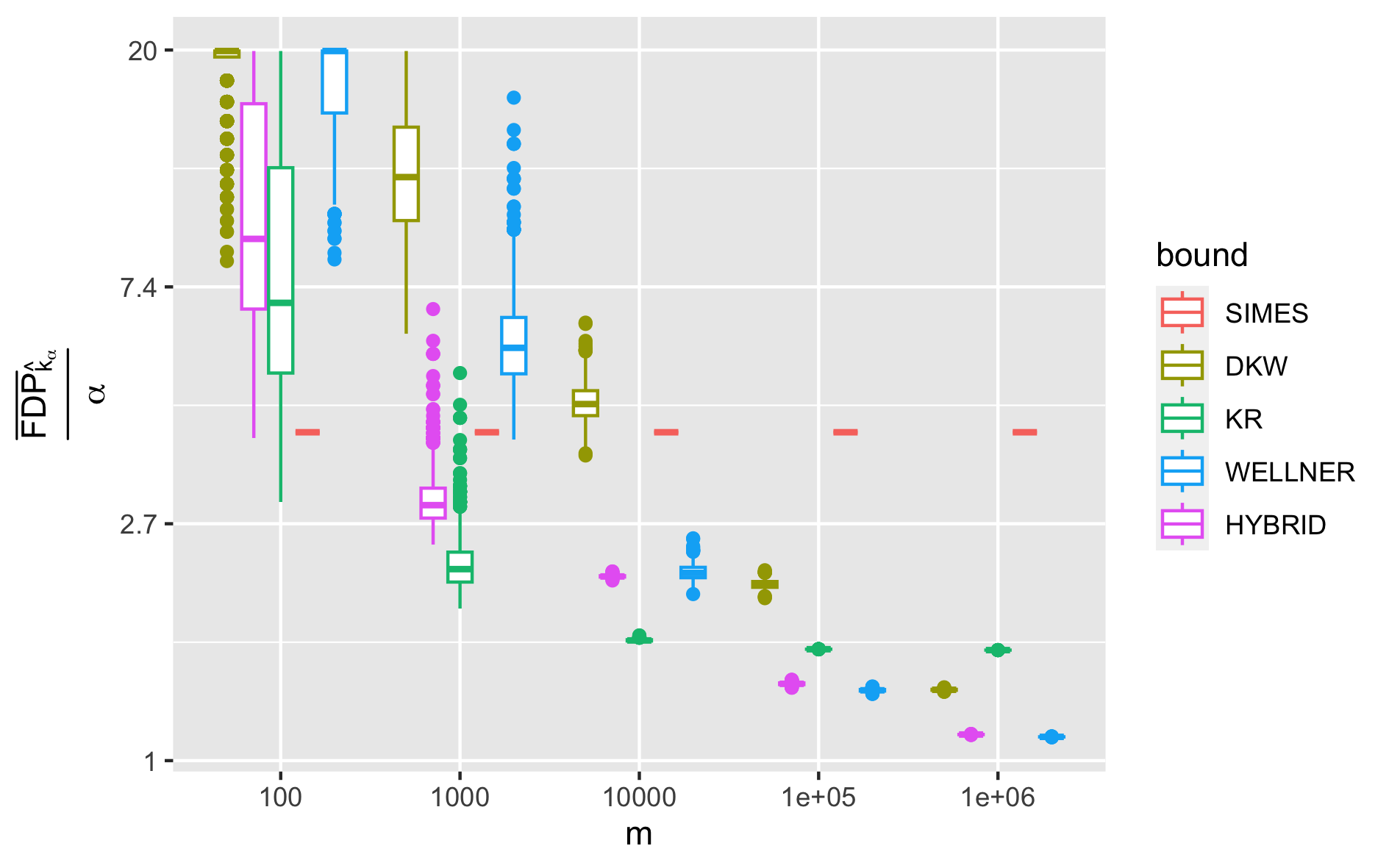
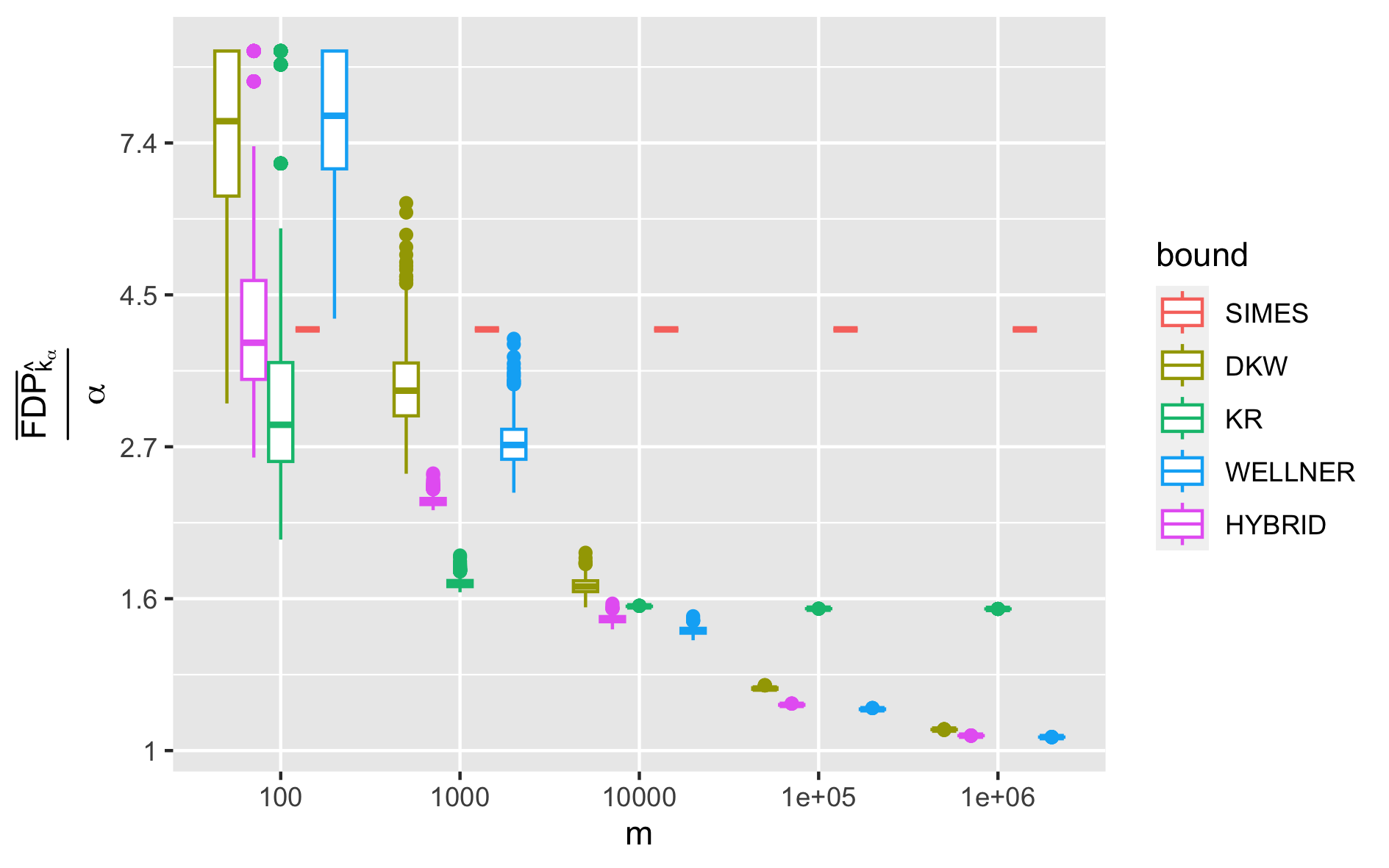
$\alpha=0.15$	$\alpha=0.2$

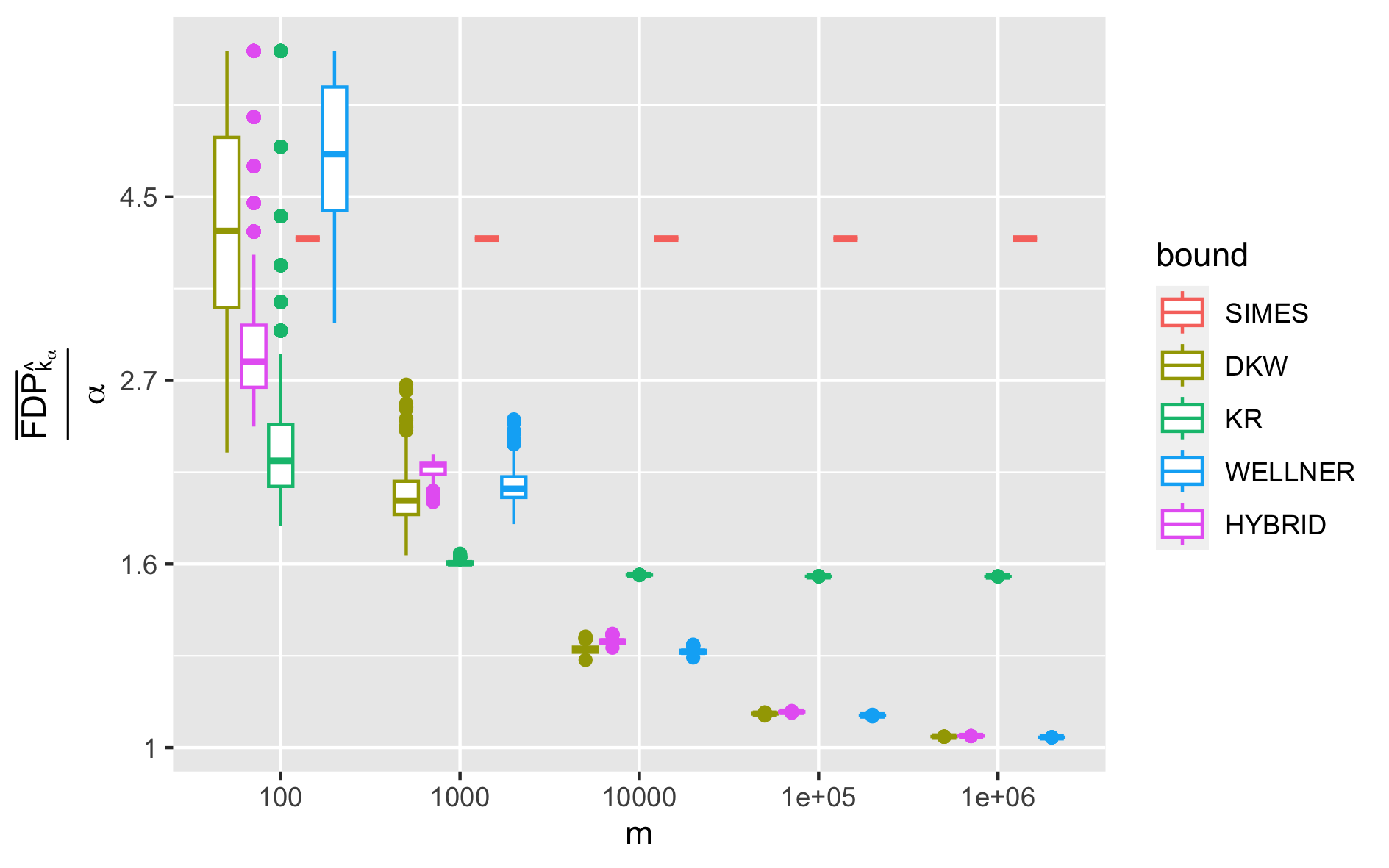
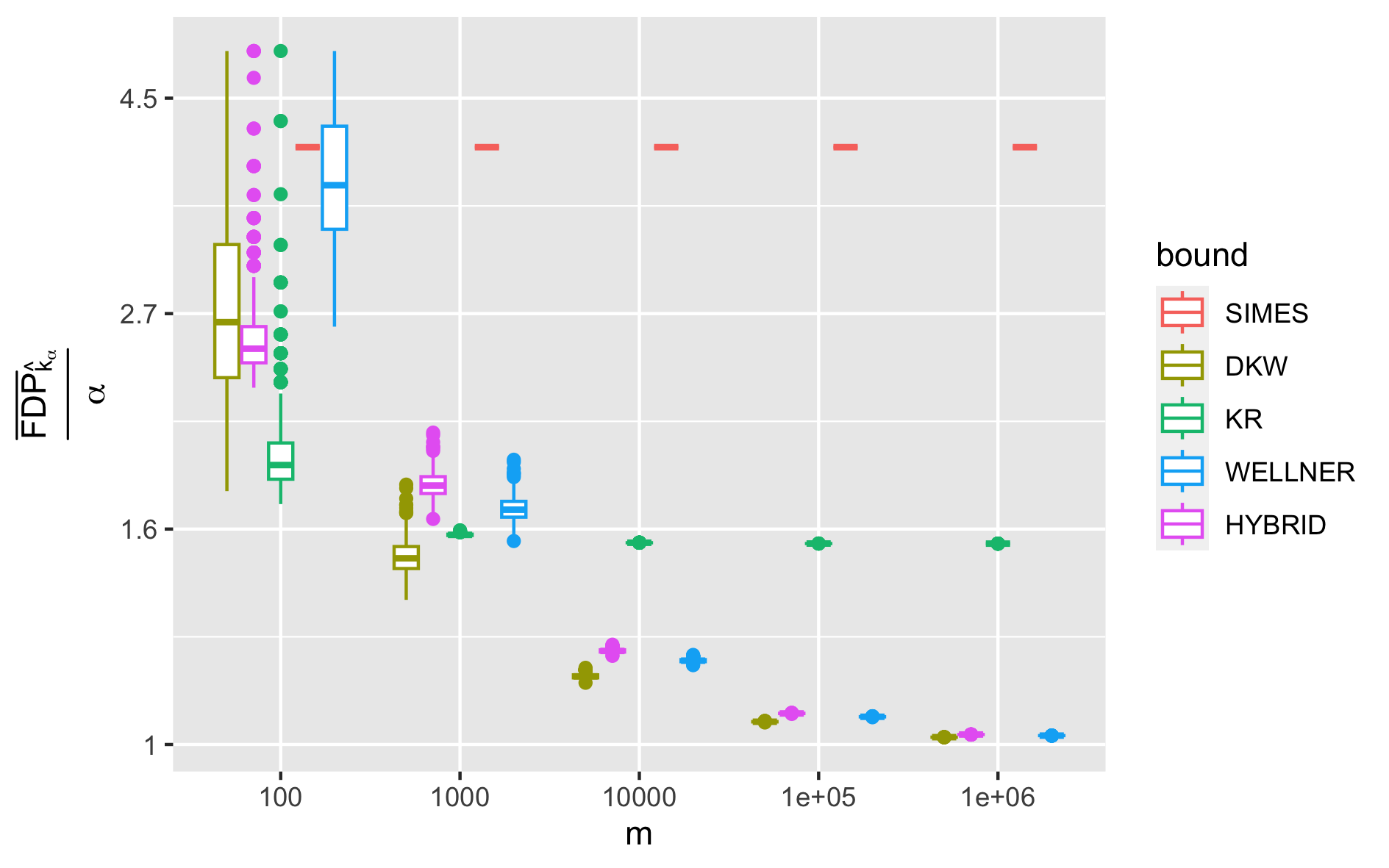
Figure 1: Top-$k$ dense case ($\pi_{0}=0.5$, $\mu=1.5$).

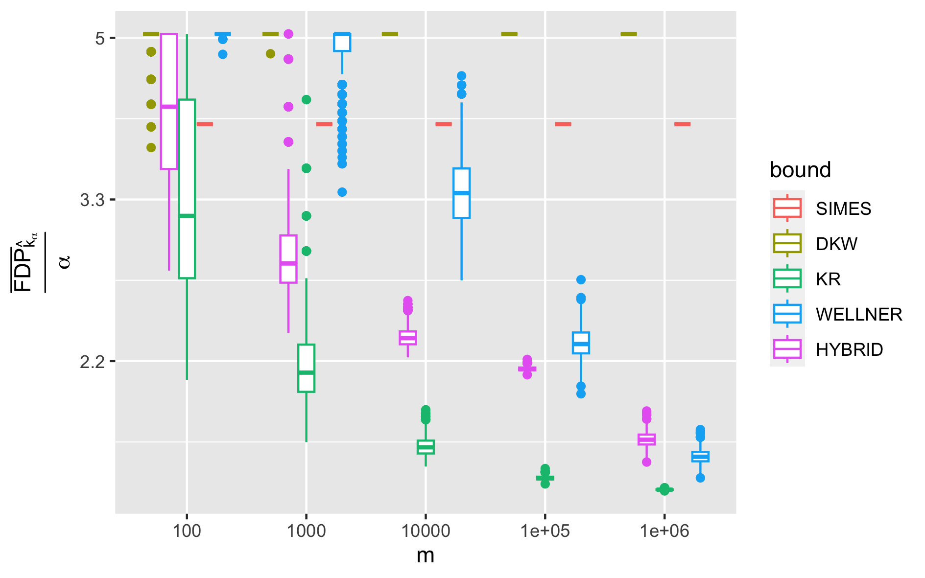
Figure 2: Top-$k$ sparse case $\pi_{0}=1-0.5m^{-0.25}$, $\mu=\sqrt{2\log(m)}$ (left) $\pi_{0}=1-0.5m^{-0.55}$, $\mu=$10 (right), $\alpha=0.2$.

Non adaptive	Adaptive

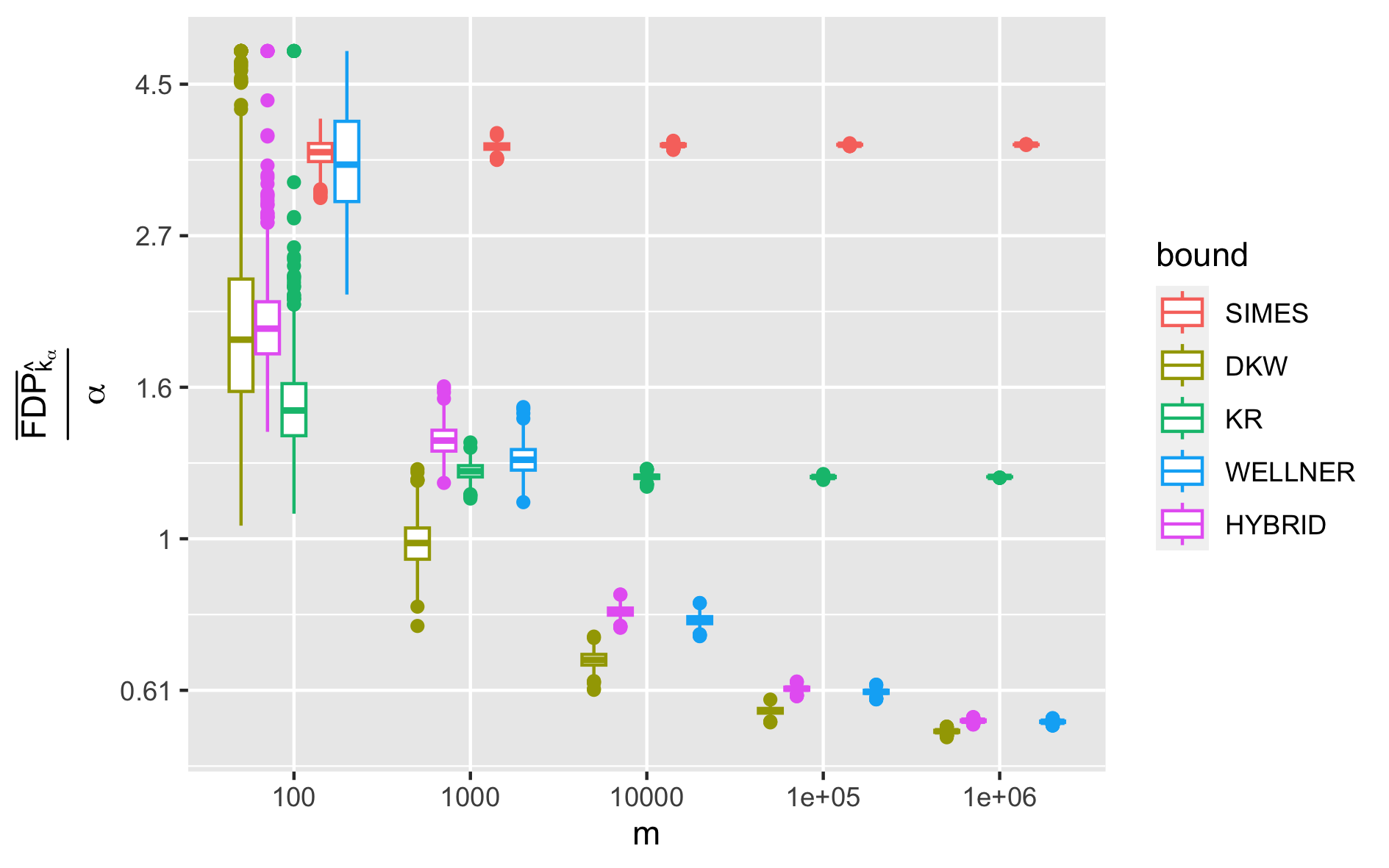
Figure 3: Top-$k$ dense case with nonadaptive bounds (left) and adaptive bounds (right) ($\pi_{0}=0.5$, $\alpha=0.2$).

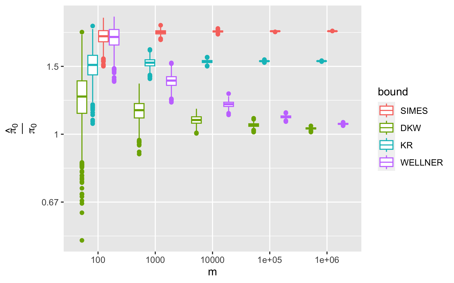
Figure 4: Boxplots of the estimators $\hat{\pi}_{0}$ in the top-$k$ dense case ($\pi_{0}=0.5$, $\alpha=0.2$).

Remark 5.1.

For clarity, the bounds are displayed without the interpolation improvement (2) (for top-$k$ and preordered). The figures are reproduced together with the interpolated bounds in Appendix E for completeness. In a nutshell, the interpolation operation improves significantly the bounds mainly when they are not very sharp (typically small $m$ or very sparse scenarios). Hence, while it can be useful in practice, it does not seem particularly relevant to study the consistency phenomenon.

5.2 Pre-ordered

We consider data generated as in the pre-ordered model presented in Section 3.1 and more specifically as in the VCT model of Section A.2. The trueness/falseness of null hypotheses are generated independently, and the probability of generating an alternative is decreasing with the position $1\leq k\leq m$, and is given by $\pi(m^{\beta-1}k)$, where $\pi:[0,\infty)\to[0,1)$ is some function (see below) and $\beta\in[0,1)$ is the sparsity parameter. Once the process of true/false nulls is given, the $p$-values are generated according to either:

• LF setting: $\pi(t)=\pi_{1}e^{-bt}\frac{b}{1-e^{-b}}$, $t\geq 0$, so that $\Pi(1)=\pi_{1}$. Here $\pi_{1}$ is equal to $0.4$ and $b$, measuring the quality of the prior ordering, is equal to $2$. In addition, the alternative $p$-values are one-sided Gaussian with $\mu=1.5$. Note that this is the setting considered in the numerical experiments of Lei and Fithian, (2016).

• Knockoff setting: $\pi(t)=1/2+(0\vee 1/2(\frac{z-t}{z-1}))$, $t\geq 0$, with $z>1$ a parameter that determines how slowly the probability of observing signal deteriorates, taken equal to $30$. Then, the binary $p$-values are as follows: under the null $p_{i}=1/2$ or $1$ with equal probability. Under the alternative, $p_{i}=1/2$ with probability $0.9$ and $p_{i}=1$ otherwise.

In both settings, the dense (resp. sparse) case refers to the sparsity parameter value $\beta=0$ (resp. $\beta=0.25$).

We consider the bounds $\overline{\textnormal{FDP}}^{\mbox{\tiny KR}}_{\alpha}$ (36), $\overline{\textnormal{FDP}}^{{\tiny\mbox{Freed}}}_{\alpha}$ (37) and $\overline{\textnormal{FDP}}_{\alpha}^{{\tiny\mbox{KR-U}}}$ (38) for the LF procedure across different values of $(\lambda,s)\in\{(1/2,0.1\alpha),(1/2,1/2)\}$, $m\in\{10^{i},2\leq i\leq 6\}$, and $\alpha\in\{0.05,0.1,0.15,0.2\}$. The procedure LF with $(\lambda,s)=(1/2,1/2)$ is referred to as the Barber and Candès (BC) procedure.

Figure 5 displays the boxplots of these FDP bounds for the LF procedure with $(\lambda,s)=(1/2,0.1\alpha)$ in the LF setting with $\beta=0$ (dense case). It is apparent that KR is not consistent, while the new bounds Freedman and KR-U are. Also, the bound KR-U is overall the best, losing almost nothing w.r.t. KR when the number of rejections is very small (say $m=100$ and $\alpha=0.05$ or $0.1$) and making a very significant improvement otherwise. Similar conclusions hold for the case of BC procedure, see Figure 7. Next, to stick with a very common scenario, we also investigate the sparse situation where the fraction of signal is small in the data, see Figures 6 and 8. As expected, while the conclusion is qualitatively the same, the rejection number gets smaller so that the consistency is reached for largest values of $m$ (i.e., the convergence is ‘slowed down’).

$\alpha=0.05$	$\alpha=0.1$
$\alpha=0.15$	$\alpha=0.2$

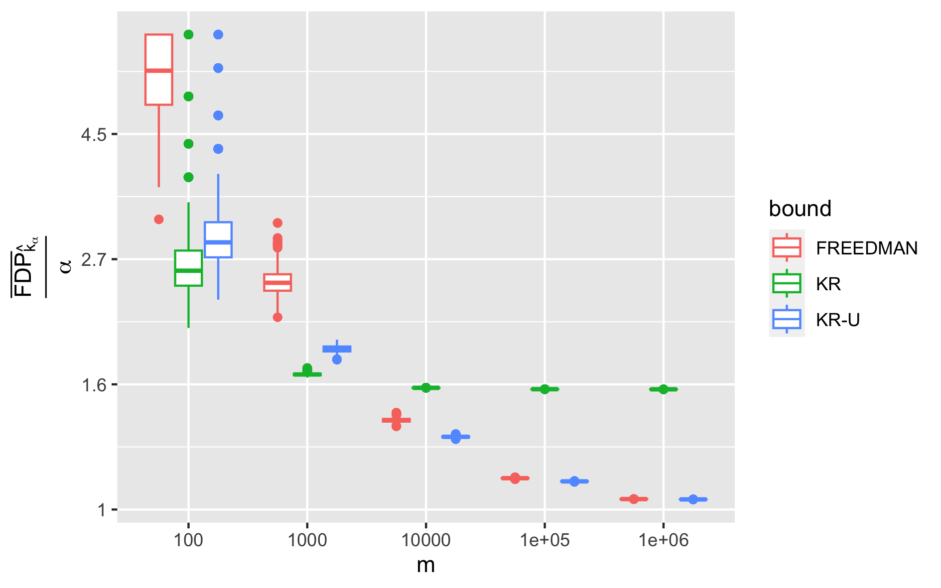
Figure 5: Preordered dense ($\beta=0$) LF setting with LF procedure ($s=0.1\alpha$, $\lambda=0.5$).

$\alpha=0.05$	$\alpha=0.1$
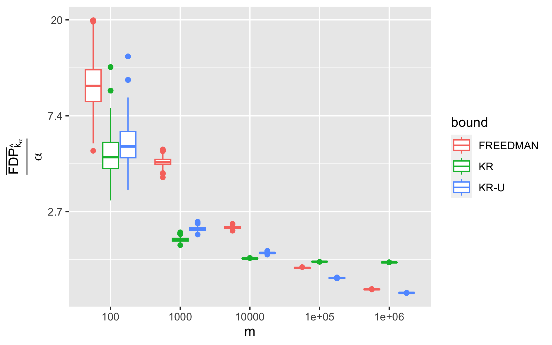
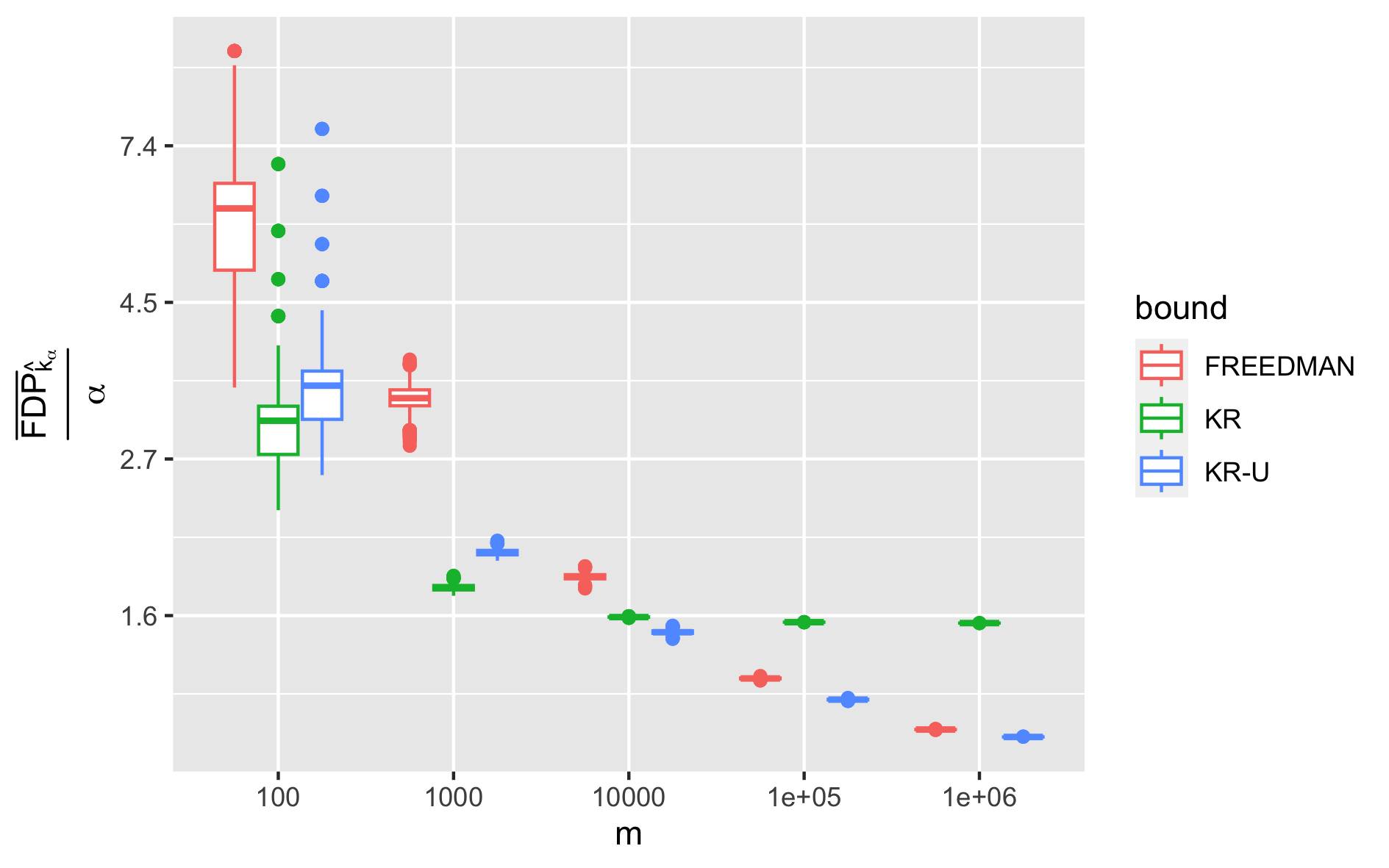
$\alpha=0.15$	$\alpha=0.2$

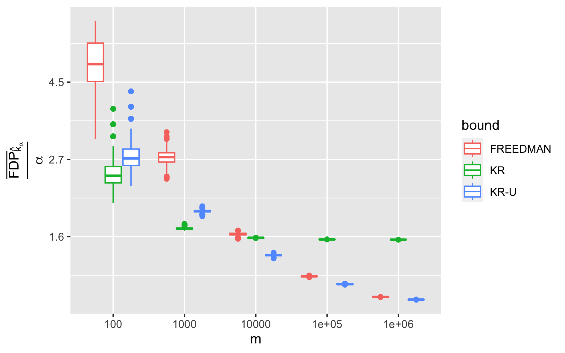
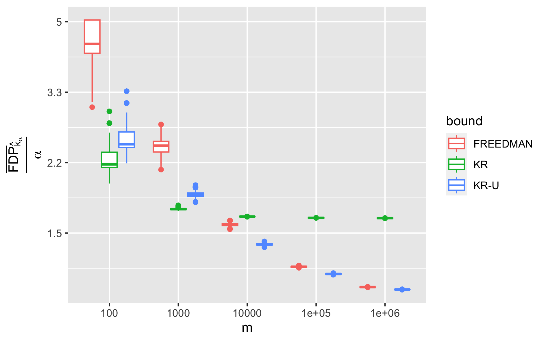
Figure 6: Preordered sparse ($\beta=0.25$) LF setting with LF procedure ($s=0.1\alpha$, $\lambda=0.5$).

$\alpha=0.15$	$\alpha=0.2$

Figure 7: Pre-ordered dense ($\beta=0$) knockoff setting with BC procedure (i.e., LF procedure with $s=\lambda=0.5$).

$\alpha=0.15$	$\alpha=0.2$

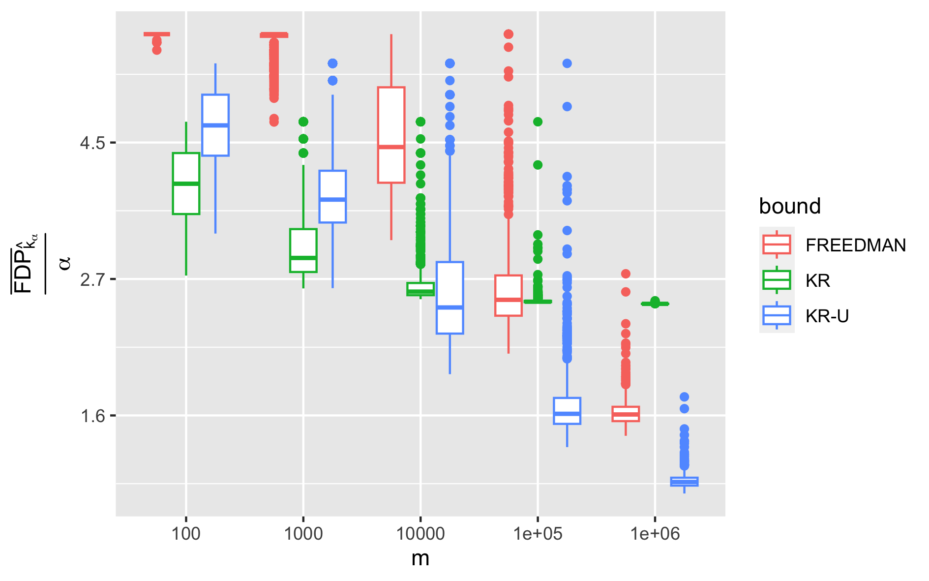
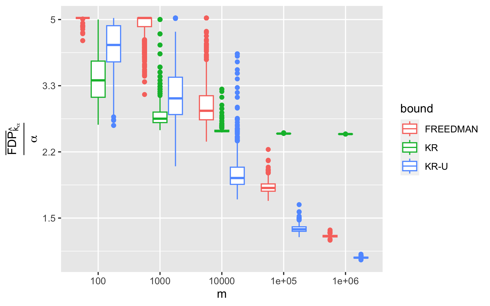
Figure 8: Pre-ordered sparse ($\beta=0.25$) knockoff setting with BC procedure (i.e., LF procedure with $s=\lambda=0.5$).

5.3 Online

We now consider the online case, by applying our method to the real data example coming from the International Mice Phenotyping Consortium (IMPC) (Muñoz-Fuentes et al.,, 2018), which is a consortium interested in the genotype effect on the phenotype. This data is collected in an online fashion for each gene of interest and is classically used in online detection works (see Ramdas et al., (2017) and references therein).

Figure 9 displays the FDP time-wise envelopes $k\mapsto\overline{\textnormal{FDP}}^{\mbox{\tiny KR}}_{\alpha,k}$ (47), $k\mapsto\overline{\textnormal{FDP}}^{{\tiny\mbox{Freed}}}_{\alpha,k}$ (48) and $k\mapsto\overline{\textnormal{FDP}}^{{\tiny\mbox{KR-U}}}_{\alpha,k}$ (49), for the LORD procedure (42) ($W_{0}=\alpha/2$ with the spending sequence $\gamma_{k}=k^{-1.6}$, $k\geq 1$). As we can see, the Freedman and KR-U envelopes both tend to the nominal level $\alpha$, as opposed to the KR envelope, which is well expected from the consistency theory. In addition, KR-U seems to outperform the Freedman envelope and while KR is (slightly) better than KR-U in the initial segment of the process $(k<300)$, we can see that KR-U gets rapidly more accurate.

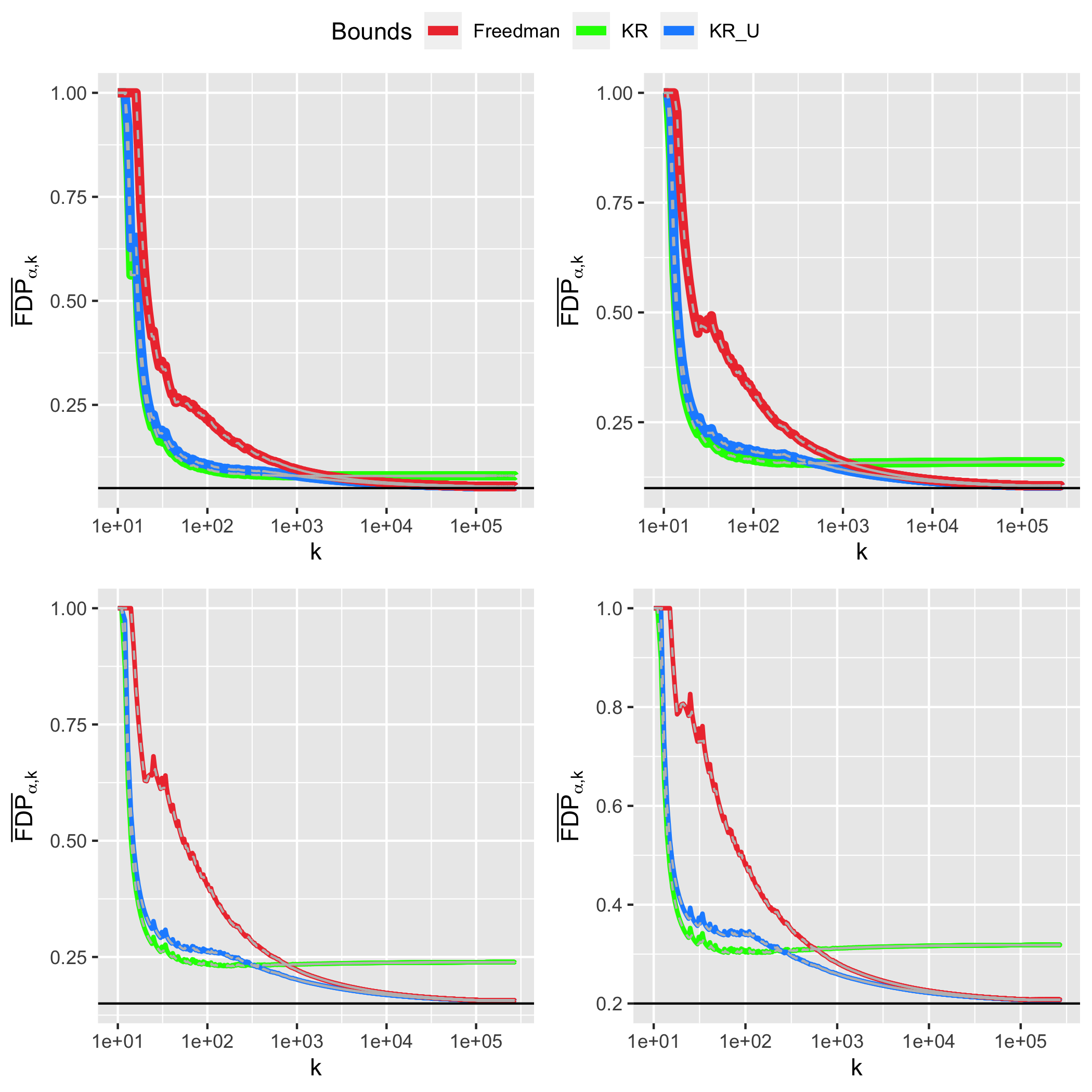
Figure 9: Online FDP envelopes for LORD applied on IMPC data for four values of $\alpha\in\{0.05,0.1,0.15,0.2\}$ (horizontal black bars). The interpolated bounds are displayed for each procedure as a gray dashed line.

5.4 Comparison to Li et al., (2022)

In this section, we compare the performances of the KR-U bound with respect to the recent bounds proposed in Li et al., (2022). For this, we reproduce the high dimensional Gaussian linear regression setting of Section 5.1 (a) therein, which generates binary $p$-values by applying the fixed-$X$ ‘sdp’ knockoffs and the signed maximum lambda knockoff statistic of Barber and Candès, (2015). Doing so, the $p$-values follow the preordered setting of Section 3.1 and thus our bounds are non-asymptotically valid (note however that the $p$-values do not follow strictly speaking the VCT model of Section A.2). To be more specific, the considered Gaussian linear model $Y\sim\mathcal{N}(X\beta,I_{n})$ is obtained by first generating $X$ and $\beta$ as follows: the correlated design matrix $X$ of size $n\times m$ is obtained by drawing $n=1500$ i.i.d. samples from the multivariate $m$-dimensional distribution $\mathcal{N}_{m}(0,\Sigma)$ where $\Sigma_{i,j}=0.6^{|i-j|}$, $1\leq i,j\leq m$; the signal vector $\beta\in\mathbb{R}^{m}$ is obtained by first randomly sampling a subset of $\{1,\dots,m\}$ of size $\lfloor\pi_{1}m\rfloor$ for the non-zero entries of $\beta$ and then by setting all non-zero entries of $\beta$ equal to $a/\sqrt{n}$ for a given amplitude $a>0$.

First, in the spirit of Figure 3 in Li et al., (2022), we display in Figure 10 the envelope $({\widetilde{\textnormal{FDP}}}_{k}^{{\tiny\mbox{KR-U}}},k\geq 1)$ given by the interpolation (2) of the envelope $(\overline{\textnormal{FDP}}_{k}^{{\tiny\mbox{KR-U}}},k\geq 1)$ defined by (35) (with $s=\lambda=1/2$), and compare it to those obtained in Li et al., (2022) (namely, KJI A/B/C/D) for $\pi_{1}\in\{0.1,0.5\}$, $a\in\{15,25\}$. We also set here $\delta=0.05$ to stick with the choice of Li et al., (2022) (note that this requires to further calibrate the parameters of their method according to this value of $\delta$) and the number of replications is here only taken equal to $10$ for computational reasons. Markedly, the KR-U envelope becomes much better than KR and is competitive w.r.t. KJI A/B/C/D, at least when $k$ is moderately large. As expected, the most favorable case for KR-U is when the signal has a large amplitude and is dense.

Second, to stick with the consistency-oriented plots of the previous sections, we also display the corresponding FDP bounds for the BC procedure at level $\alpha\in\{0.15,0.2\}$ in Figure 11. The conclusions are qualitatively similar.

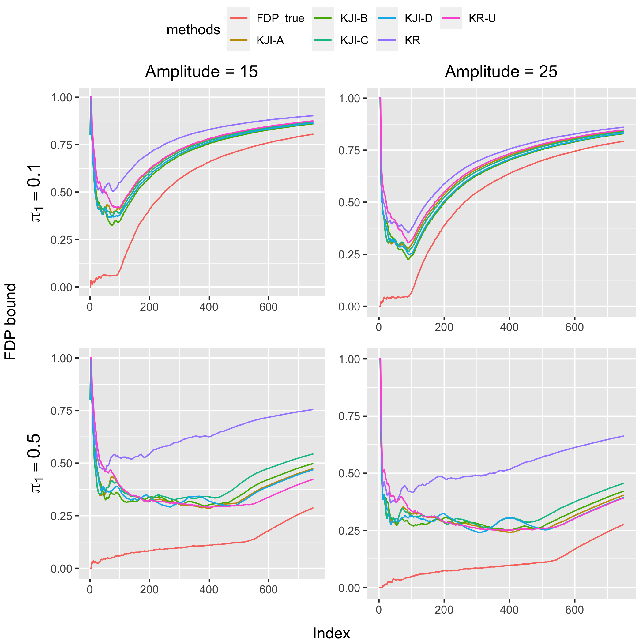
Figure 10: Comparing the envelope ${\widetilde{\textnormal{FDP}}}_{k}^{{\tiny\mbox{KR-U}}}$, $k\geq 1$ given by (2)-(35) ($s=\lambda=0.5$) to those of Li et al., (2022) in the Gaussian linear regression setting of Section 5.4 for $m=1000$ (see text for more details).

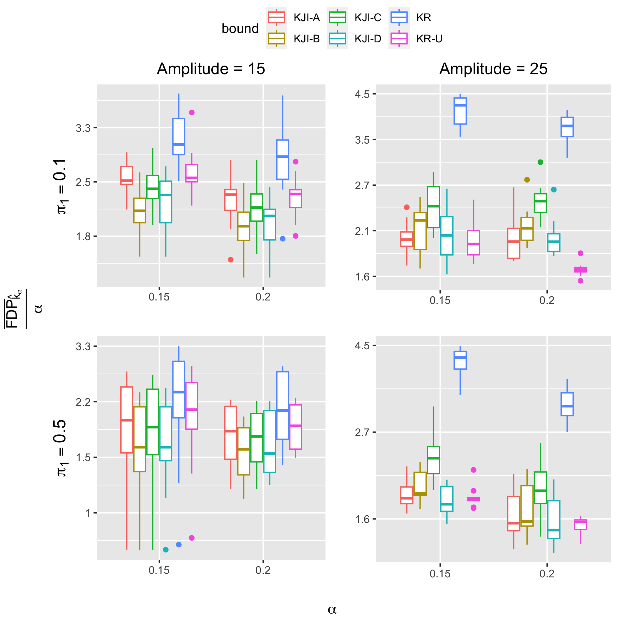
Figure 11: Comparing the FDP bound ${\widetilde{\textnormal{FDP}}}_{\hat{k}_{\alpha}}^{{\tiny\mbox{KR-U}}}$ for $\hat{k}_{\alpha}$ the BC procedure (32) ($s=\lambda=0.5$) to those of Li et al., (2022) with respect to $\alpha\in\{0.15,0.2\}$ in the Gaussian linear regression setting of Section 5.4 for $m=1000$ (see text for more details).

6 Conclusion

The main point if this paper is to provide another point of view on FDP confidence bounds: we introduced a notion of consistency, a desirable asymptotical property which should act as a guiding principle when building such bounds, by ensuring that the bound is sharp enough on particular FDR controlling rejection sets. Doing so, some previous bounds were shown to be inconsistent, as the original KR bounds; while some other known FDP confidence bounds, in particular based on the DKW inequality, are consistent under certain assumptions, we have introduced new ones shown to satisfy this condition under more general conditions (in particular high sparsity). New bounds based on the classical Wellner/Freedman inequalities showed interesting behaviors, however simple modifications of KR bounds Hybrid/KR-U by ‘stitching’ have been shown to be the most efficient, both asymptotically and for moderate sample size.

Overall, this work shows that consistency is a simple and fruitful criterion, and we believe that using it will be beneficial in the future to make wise choices among the rapidly increasing literature on FDP bounds.

Appendix A Power results

A.1 Top-$k$ setting

Definition A.1.

The sparse one-sided Gaussian location model of parameter $m,b,c,\beta$, denoted as $\mathbf{P}^{(m)}_{b,c,\beta}$, is defined as follows: $p_{i}=\overline{\Phi}(X_{i})$, $1\leq i\leq m$, the $X_{i}$’s are independent, with $X_{i}\sim\mathcal{N}(0,1)$ for $i\in{\mathcal{H}}_{0}$ and $X_{i}\sim\mathcal{N}(\mu_{m},1)$ otherwise, for $\mu_{m}=\sqrt{2\beta\log m}+b$, $b>0$, and $m_{1}=|{\mathcal{H}}_{1}|=cm^{1-\beta}$, $c\in(0,1)$, $\beta\in[0,1)$.

Note that $\beta=0$ is the dense case for which the alternative mean $\mu_{m}=b>0$ is a fixed quantity, whereas $\beta>0$ in the sparse case, for which $\mu_{m}=\sqrt{2\beta\log m}+b$ tends to infinity. In both case, the magnitude of alternative mean is defined to be on the ‘verge of detectability’ where the BH procedure has some non-zero power, see Bogdan et al., (2011); Neuvial and Roquain, (2012); Abraham et al., (2021) for instance.

Theorem A.2.

Let $\alpha\in(0,1)$. In the above one-sided Gaussian location model $\mathbf{P}^{(m)}_{b,c,\beta}$, the number of rejections $\hat{k}_{\alpha}$ of the BH procedure is such that, as $m$ grows to infinity,

$$\mathbf{P}^{(m)}_{b,c,\beta}(t^{*}_{m}\leq\alpha\hat{k}_{\alpha}/m\leq t^{\sharp}_{m})\geq 1-2e^{-dm_{1}},\mbox{ for }m_{1}/m\lesssim t^{*}_{m}\leq t^{\sharp}_{m}\lesssim m_{1}/m,$$ (50)

for some constant $d>0$ (depending on $\alpha$, $\beta$, $b$), where $t^{*}_{m}\in(0,1)$ is the unique solution of $G_{m}(t)=2t/\alpha$, $t^{\sharp}_{m}\in(0,1)$ is the unique solution of $G_{m}(t)=0.5t/\alpha$, and where $G_{m}(t)=(m_{0}/m)t+(m_{1}/m)\overline{\Phi}(\overline{\Phi}^{-1}(t)-\mu_{m})$, with $\overline{\Phi}(z)=\mathbf{P}(Z\geq z)$, $z\in\mathbb{R}$.

Proof.

First let $F_{m}(t)=\overline{\Phi}(\overline{\Phi}^{-1}(t)-\mu_{m})$, $\Psi_{m}(t)=F_{m}(t)/t$ and observe that $\Psi_{m}$ is continuous decreasing on $(0,1]$ with $\lim_{0}\Psi_{m}=+\infty$. This implies that $t^{*}_{m},t^{\sharp}_{m}\in(0,1)$ as described in the statement both exist, with

$$t^{*}_{m}=\Psi_{m}^{-1}(\alpha/2),\>\>t^{\sharp}_{m}=\Psi_{m}^{-1}(\tau_{m}(2\alpha)),\>\>\tau_{m}(\alpha)=\frac{m}{m_{1}}\mathopen{}\mathclose{{}\left(\frac{1}{\alpha}-\frac{m_{0}}{m}}\right).$$

We first establish

$$t^{*}_{m}\gtrsim m_{1}/m$$ (51)

$$t^{\sharp}_{m}\lesssim m_{1}/m.$$ (52)

If $\beta=0$, then $m_{0}/m=1-c$, $m_{1}/m=c$, $\mu_{m}=b$, $\tau_{m}>0$, $F_{m}(t)=\overline{\Phi}(\overline{\Phi}^{-1}(t)-b)$, $\Psi_{m}(t)=\overline{\Phi}(\overline{\Phi}^{-1}(t)-b)/t$, $\tau_{m}(\alpha)$ all do not depend on $m$. Hence, $t^{*}_{m}$ and $t^{\sharp}_{m}$ are both constant, which establishes (51) and (52). Let us now turn to the sparse case, for which $\beta\in(0,1)$. The inequality (52) follows from the upper bound

$$0.5t^{\sharp}_{m}/\alpha=G_{m}(t^{\sharp}_{m})\leq t^{\sharp}_{m}+m_{1}/m.$$

For (51), the analysis is slightly more involved. We first prove that for $m$ large enough

$$\overline{\Phi}^{-1}(t_{m}^{*})\leq\mu_{m}-b.$$ (53)

This will establish (51), since it implies $F_{m}(t_{m}^{*})\geq F_{m}(\overline{\Phi}(\mu_{m}-b))=\overline{\Phi}(-b)>0$ and also $t_{m}^{*}=(\tau_{m}(\alpha/2))^{-1}F_{m}(t^{*}_{m})\gtrsim m_{1}/m$. On the one hand,

$$\Psi_{m}(\overline{\Phi}(\mu_{m}-b))=\frac{\overline{\Phi}(-b)}{\overline{\Phi}(\mu_{m}-b)}\geq\overline{\Phi}(-b)\frac{\mu_{m}-b}{\phi(\mu_{m}-b)}=\Phi(-b)m^{\beta}\sqrt{2\beta\log m}$$

because $\mu_{m}-b=\sqrt{2\beta\log m}$ and $\phi(\mu_{m}-b)=m^{-\beta}$, and by using $\Phi(x)\leq\phi(x)/x$ for all $x>0$. On the other hand,

$$\Psi_{m}(t_{m}^{*})=\tau_{m}(\alpha/2)\leq\frac{2}{\alpha}m^{\beta}.$$

Hence, for $m$ large enough, we have $\Psi_{m}(\overline{\Phi}(\mu_{m}-b))\geq\Psi_{m}(t_{m}^{*})=\Psi_{m}(\overline{\Phi}(\overline{\Phi}^{-1}(t_{m}^{*})))$, which in turn implies (53).

We now turn to prove the result (50) and follow for a classical concentration argument. Let

$$\hat{G}_{m}(t)=m^{-1}\sum_{i=1}^{m}{\bm{1}\IfEqCase{a}{{a}{\mathopen{}\mathclose{{}\left\{p_{i}\leq t}\right\}}{0}{\{p_{i}\leq t\}}{1}{\big{\{}p_{i}\leq t\big{\}}}{2}{\Big{\{}p_{i}\leq t\Big{\}}}{3}{\bigg{\{}p_{i}\leq t\bigg{\}}}{4}{\Bigg{\{}p_{i}\leq t\Bigg{\}}}}[]},\>\>\>t\in[0,1],$$

so that $G_{m}(t)=\mathbf{E}\hat{G}_{m}(t)$ for all $t\in[0,1]$. Hence, for all $t\in(0,1)$,

$$\mathbf{P}(\alpha\hat{k}_{\alpha}/m<t) \leq\mathbf{P}\mathopen{}\mathclose{{}\left(\hat{G}_{m}(t)\leq t/\alpha}\right)$$

$$=\mathbf{P}\mathopen{}\mathclose{{}\left(\hat{G}_{m}(t)-G_{m}(t)\leq t/\alpha-G_{m}(t)}\right),$$

because $\alpha\hat{k}_{\alpha}/m=\max\{t\in(0,1)\>:\>\hat{G}_{m}(t)\geq t/\alpha\}$ by definition of $\hat{k}_{\alpha}$. Applying this with $t=t^{*}_{m}$, this gives

$$\mathbf{P}(\alpha\hat{k}_{\alpha}/m<t^{*}_{m}) =\mathbf{P}\mathopen{}\mathclose{{}\left(\hat{G}_{m}(t^{*}_{m})-G_{m}(t^{*}_{m})\leq-G_{m}(t^{*}_{m})}\right)$$

$$\leq\exp\mathopen{}\mathclose{{}\left(-cmG_{m}(t^{*}_{m})}\right)\leq\exp\mathopen{}\mathclose{{}\left(-Cm_{1}F_{m}(t^{*}_{m})}\right),$$

for some constant $C>0$, by applying Bernstein’s inequality. Since $F_{m}(t_{m}^{*})\geq\overline{\Phi}(-b)>0$, this gives $\mathbf{P}(\alpha\hat{k}_{\alpha}/m<t^{*}_{m})\leq e^{-dm_{1}}$ for $m$ large enough and some constant $d>0$.

Next, for all $t\in[t^{\sharp}_{m},1)$, still applying Bernstein’s inequality,

$$\mathbf{P}(\alpha\hat{k}_{\alpha}/m>t)$$

$$\leq\sum_{k=1}^{m}{\bm{1}\IfEqCase{a}{{a}{\mathopen{}\mathclose{{}\left\{\alpha k/m>t}\right\}}{0}{\{\alpha k/m>t\}}{1}{\big{\{}\alpha k/m>t\big{\}}}{2}{\Big{\{}\alpha k/m>t\Big{\}}}{3}{\bigg{\{}\alpha k/m>t\bigg{\}}}{4}{\Bigg{\{}\alpha k/m>t\Bigg{\}}}}[]}\mathbf{P}\mathopen{}\mathclose{{}\left(\hat{G}_{m}(\alpha k/m)-{G}_{m}(\alpha k/m)\geq k/m-{G}_{m}(\alpha k/m)}\right)$$

$$\leq\sum_{k=1}^{m}{\bm{1}\IfEqCase{a}{{a}{\mathopen{}\mathclose{{}\left\{\alpha k/m>t}\right\}}{0}{\{\alpha k/m>t\}}{1}{\big{\{}\alpha k/m>t\big{\}}}{2}{\Big{\{}\alpha k/m>t\Big{\}}}{3}{\bigg{\{}\alpha k/m>t\bigg{\}}}{4}{\Bigg{\{}\alpha k/m>t\Bigg{\}}}}[]}\exp\mathopen{}\mathclose{{}\left(-m\frac{(k/m-{G}_{m}(\alpha k/m))^{2}}{G_{m}(\alpha k/m)+(1/3)(k/m-{G}_{m}(\alpha k/m))}}\right)\leq m\exp\mathopen{}\mathclose{{}\left(-Cmt^{\sharp}_{m}}\right),$$

because for all $\alpha k/m\geq t^{\sharp}_{m}$, $k/m-{G}_{m}(\alpha k/m)\geq G_{m}(\alpha k/m)\geq G_{m}(t^{\sharp}_{m})=0.5t^{\sharp}_{m}/\alpha$ (given the monotonicity of $t\mapsto G_{m}(t)/t$). Applying this for $t=t^{\sharp}_{m}\in(0,1)$, we obtain

$$\mathbf{P}(\alpha\hat{k}_{\alpha}/m>t^{\sharp}_{m}) \leq e^{-dm_{1}},$$

because $t^{\sharp}_{m}\geq t^{*}_{m}\gtrsim m_{1}/m$. This proves the result.

∎

A.2 Pre-ordered setting

We introduce below a model generalizing the one of Lei and Fithian, (2016) to the possibly sparse case. Here, without loss of generality we assume that the ordering $\pi$ is identity, that is, $\pi(i)=i$ for all $i\in\{1,\dots,m\}$. Below, with some abuse, the notation $\pi$ will be re-used to stick with the notation of Lei and Fithian, (2016).

Definition A.3.

The sparse VCT model of parameters $m,\pi,\beta,F_{0},F_{1}$, denoted as $\mathbf{P}^{(m)}_{\pi,\beta,F_{0},F_{1}}$, is the $p$-value mixture model where $(p_{k},H_{k})\in[0,1]\times\{0,1\}$, $1\leq k\leq m$, are independent and generated as follows:

• the $H_{k}$, $1\leq k\leq m$, are independent and $\mathbf{P}(H_{k}=1)=\pi_{m}(k/m)$, $1\leq k\leq m$, with $\pi_{m}(x)=\pi(m^{\beta}x)$, $x\geq 0$, where $\pi:[0,\infty)\to[0,1)$ is some measurable function (instantaneous signal probability function) with $\pi(0)>0$ and $\pi(x)=\pi(1)$ for $x\geq 1$ and $\beta\in[0,1)$ is a sparsity parameter.

• conditionally on $H_{1},\dots,H_{k}$, the $p$-values $p_{k}$, $1\leq k\leq m$, are independent, with a marginal distribution super-uniform under the null: $p_{k}\>|\>H_{k}=0\sim F_{0}$, $1\leq k\leq m$, where $F_{0}$ is a c.d.f. with $F_{0}(t)\leq t$ for all $t\in[0,1]$; and $p_{k}\>|\>H_{k}=1\sim F_{1}$, $1\leq k\leq m$, where $F_{1}$ is some alternative c.d.f.

We denote $\Pi(t):=t^{-1}\int_{0}^{t}\pi(s)ds$, with $\Pi(0)=\pi(0)$ and

$$\Pi_{m}(t):=t^{-1}\int_{0}^{t}\pi_{m}(s)ds=t^{-1}\int_{0}^{t}\pi(m^{\beta}s)ds=m^{-\beta}t^{-1}\int_{0}^{m^{\beta}t}\pi(s)ds=\Pi(m^{\beta}t)$$

the expected fraction of signal before time $mt$. We also let $\pi_{1}:=\Pi_{m}(1)=\int_{0}^{1}\pi_{m}(s)ds=m^{-\beta}\Pi(1)$ the overall expected fraction of signal. We consider the asymptotic where $m$ tends to infinity and $F_{0},F_{1}$ are fixed.

When $\beta=0$, $\pi_{m}$, $\Pi_{m}$ are fixed and we recover the dense VTC model introduced in Lei and Fithian, (2016) (also noting that we are slightly more general because $F_{0}$ is possibly non-uniform and $F_{1}$ not concave). Interestingly, the above formulation can also handle the sparse case for which $\beta\in(0,1)$ and the probability to generate a signal is shrunk to $0$ by a factor $m^{\beta}$. For instance, if $\pi(1)=0$, the model only generates null $p$-values $p_{k+1},\dots,p_{m}$ for $k\geq m^{1-\beta}$.

We now analyze the asymptotic behavior of the number of rejections of the LF procedure. By following the same heuristic than in Lei and Fithian, (2016) (which follows by a concentration argument), we have from (32) that for $k=\lfloor mt\rfloor$,

$${\widehat{\textnormal{FDP}}}_{k} =\frac{s}{1-\lambda}\frac{1+\sum_{i=1}^{k}{\bm{1}\IfEqCase{a}{{a}{\mathopen{}\mathclose{{}\left\{p_{i}>\lambda}\right\}}{0}{\{p_{i}>\lambda\}}{1}{\big{\{}p_{i}>\lambda\big{\}}}{2}{\Big{\{}p_{i}>\lambda\Big{\}}}{3}{\bigg{\{}p_{i}>\lambda\bigg{\}}}{4}{\Bigg{\{}p_{i}>\lambda\Bigg{\}}}}[]}}{1\vee\sum_{i=1}^{k}{\bm{1}\IfEqCase{a}{{a}{\mathopen{}\mathclose{{}\left\{p_{i}\leq s}\right\}}{0}{\{p_{i}\leq s\}}{1}{\big{\{}p_{i}\leq s\big{\}}}{2}{\Big{\{}p_{i}\leq s\Big{\}}}{3}{\bigg{\{}p_{i}\leq s\bigg{\}}}{4}{\Bigg{\{}p_{i}\leq s\Bigg{\}}}}[]}}$$

$$\approx\frac{s}{1-\lambda}\frac{\mathopen{}\mathclose{{}\left(\sum_{i=1}^{k}(1-\pi_{m}(i/m))}\right)(1-F_{0}(\lambda))+\mathopen{}\mathclose{{}\left(\sum_{i=1}^{k}\pi_{m}(i/m)}\right)(1-F_{1}(\lambda))}{\mathopen{}\mathclose{{}\left(\sum_{i=1}^{k}(1-\pi_{m}(i/m))}\right)F_{0}(s)+\mathopen{}\mathclose{{}\left(\sum_{i=1}^{k}\pi_{m}(i/m)}\right)F_{1}(s)}$$

$$\approx\frac{1+\Pi_{m}(t)\mathopen{}\mathclose{{}\left(\frac{1-F_{1}(\lambda)}{1-\lambda}-1}\right)}{1+\Pi_{m}(t)\mathopen{}\mathclose{{}\left(\frac{F_{1}(s)}{s}-1}\right)}=\textnormal{FDP}^{\infty}(m^{\beta}t),$$

by assuming $F_{0}(s)=s$, $F_{0}(\lambda)=\lambda$, $F_{1}(s)>s$, $F_{1}(\lambda)>\lambda$ and by letting

$$\textnormal{FDP}^{\infty}(t)=\frac{1+\Pi(t)\mathopen{}\mathclose{{}\left(\frac{1-F_{1}(\lambda)}{1-\lambda}-1}\right)}{1+\Pi(t)\mathopen{}\mathclose{{}\left(\frac{F_{1}(s)}{s}-1}\right)},\>\>\>t\geq 0.$$ (54)

By (32), the quantity $\hat{k}_{\alpha}/m^{1-\beta}$ should be asymptotically close to

$$t^{*}_{\alpha}=\max\{t\in[0,+\infty)\>:\>\textnormal{FDP}^{\infty}(t)\leq\alpha\},$$ (55)

with the convention $t^{*}_{\alpha}=+\infty$ if the set is not upper bounded. We should however ensure that the latter set is not empty. For this, we let

$$\underline{\alpha} =\frac{1+\pi(0)\mathopen{}\mathclose{{}\left(\frac{1-F_{1}(\lambda)}{1-\lambda}-1}\right)}{1+\pi(0)\mathopen{}\mathclose{{}\left(\frac{F_{1}(s)}{s}-1}\right)}.$$ (56)

Hence, $\hat{r}_{\alpha}=\sum_{i=1}^{\hat{k}_{\alpha}}{\bm{1}\IfEqCase{a}{{a}{\mathopen{}\mathclose{{}\left\{p_{i}\leq s}\right\}}{0}{\{p_{i}\leq s\}}{1}{\big{\{}p_{i}\leq s\big{\}}}{2}{\Big{\{}p_{i}\leq s\Big{\}}}{3}{\bigg{\{}p_{i}\leq s\bigg{\}}}{4}{\Bigg{\{}p_{i}\leq s\Bigg{\}}}}[]}$, the number of rejections of LF procedure, should be close to $\mathopen{}\mathclose{{}\left(\sum_{i=1}^{\hat{k}_{\alpha}}(1-\pi_{m}(i/m))}\right)F_{0}(s)+\mathopen{}\mathclose{{}\left(\sum_{i=1}^{\hat{k}_{\alpha}}\pi_{m}(i/m)}\right)F_{1}(s)\gtrsim\hat{k}_{\alpha}s\approx m^{1-\beta}t^{*}_{\alpha}s$. This heuristic is formalized in the next result.

Theorem A.4.

Consider a sparse VCT model $\mathbf{P}^{(m)}_{\pi,\beta,F_{0},F_{1}}$ with parameters $\beta,\pi,F_{0},F_{1}$ (see Definition A.3) and the LF procedure with parameter $s,\lambda$ (see (32)), with the assumptions:

• $\Pi:t\in[0,\infty)\to\mathbb{R}_{+}$ is continuous decreasing and $L$-Lipschitz;

• $F_{0}(s)=s$, $F_{0}(\lambda)=\lambda$, $F_{1}(s)>s$, $F_{1}(\lambda)>\lambda$;

• $\alpha>\underline{\alpha}$ where $\underline{\alpha}$ is defined by (56).

Let $\alpha^{\prime}=(\underline{\alpha}+\alpha)/2\in(\underline{\alpha},\alpha)$, $t^{*}_{\alpha^{\prime}}\in(0,+\infty]$ given by (55), $t^{*}_{m}=t^{*}_{\alpha^{\prime}}\wedge m^{\beta}$ and let $a\geq 1$ be an integer $a\leq m^{1-\beta}t^{*}_{m}$ such that $r=\frac{4}{a^{1/4}}\mathopen{}\mathclose{{}\left(\frac{1}{s}+\frac{1}{1-\lambda}}\right)$ is small enough to provide $r\leq(\alpha-\underline{\alpha})/4$. Then the number of rejections $\hat{r}_{\alpha}=\sum_{i=1}^{\hat{k}_{\alpha}}{\bm{1}\IfEqCase{a}{{a}{\mathopen{}\mathclose{{}\left\{p_{i}\leq s}\right\}}{0}{\{p_{i}\leq s\}}{1}{\big{\{}p_{i}\leq s\big{\}}}{2}{\Big{\{}p_{i}\leq s\Big{\}}}{3}{\bigg{\{}p_{i}\leq s\bigg{\}}}{4}{\Bigg{\{}p_{i}\leq s\Bigg{\}}}}[]}$ of the LF procedure (32) is such that

$$\mathbf{P}^{(m)}_{\pi,\beta,F_{0},F_{1}}(\hat{r}_{\alpha}<r_{m}^{*})\leq 2(2+a^{1/2})e^{-2a^{1/2}},\>\>\>\>r^{*}_{m}=\lfloor m^{1-\beta}t^{*}_{m}\rfloor s/2.$$ (57)

In particular, choosing $a=1+\lfloor(\log m)^{2}\rfloor$, we have as $m$ grows to infinity, $m^{1-\beta}/\hat{r}_{\alpha}=O_{P}(1).$

Condition (ii) is more general that in Lei and Fithian, (2016) and allows to handle binary $p$-values, like in the ‘knockoffs’ situation (for which $F_{0}$ and $F_{1}$ are not continuous). The condition (iii) was overlooked in Lei and Fithian, (2016), but it is needed to ensure the existence of $t^{*}_{\alpha}$. It reads equivalently

$$\pi(0)>\frac{1-\alpha}{1-\frac{1-F_{1}(\lambda)}{1-\lambda}+\alpha\mathopen{}\mathclose{{}\left(\frac{F_{1}(s)}{s}-1}\right)},$$ (58)

which provides that the probability to generate a null is sufficiently large at the beginning of the $p$-value sequence, with a minimum amplitude function of $F_{1}(s)$ and $F_{1}(\lambda)$. Note that in the ‘knockoffs’ case where $s=\lambda=1/2$, we have $\underline{\alpha}=\frac{1-\pi(0)M}{1+\pi(0)M}$ where $M=2F_{1}(1/2)-1>0$ can be interpreted as a ‘margin’. Hence, the critical level $\underline{\alpha}$ is decreasing in $\pi(0)M$. Hence, the setting is more favorable either when $\pi(0)$ increases, or when the margin $M$ increases.

Proof.

First note that $\textnormal{FDP}^{\infty}(t)$ is an decreasing function of $\Pi(t)$ because $\frac{1-F_{1}(\lambda)}{1-\lambda}<1<\frac{F_{1}(s)}{s}$, see (54). Since $\Pi(t)$ is decreasing from $\pi(0)$ to $\pi(1)=\Pi(+\infty)$, we have that $\textnormal{FDP}^{\infty}:[0,+\infty)\to[\underline{\alpha},\overline{\alpha}]$ is continuous increasing, where $\overline{\alpha}=\mathopen{}\mathclose{{}\left(1+\pi(1)\mathopen{}\mathclose{{}\left(\frac{1-F_{1}(\lambda)}{1-\lambda}-1}\right)}\right))/\mathopen{}\mathclose{{}\left(1+\pi(1)\mathopen{}\mathclose{{}\left(\frac{F_{1}(s)}{s}-1}\right)}\right)$. Hence, if $\alpha^{\prime}<\overline{\alpha}$, we have $0<t^{*}_{\alpha^{\prime}}<+\infty$, $t^{*}_{m}=t^{*}_{\alpha^{\prime}}$ for $m$ large enough, and thus $\textnormal{FDP}^{\infty}(t^{*}_{m})=\alpha^{\prime}$. If $\alpha^{\prime}\geq\overline{\alpha}$, $t^{*}_{\alpha^{\prime}}=+\infty$, $t^{*}_{m}=m^{\beta}$ and $\textnormal{FDP}^{\infty}(t^{*}_{m})\leq\alpha^{\prime}$. Both cases are considered in what follows. Consider the events

$$\Omega_{1} =\mathopen{}\mathclose{{}\left\{\sup_{a\leq k\leq m}\mathopen{}\mathclose{{}\left|k^{-1}\sum_{i=1}^{k}{\bm{1}\IfEqCase{a}{{a}{\mathopen{}\mathclose{{}\left\{p_{i}>\lambda}\right\}}{0}{\{p_{i}>\lambda\}}{1}{\big{\{}p_{i}>\lambda\big{\}}}{2}{\Big{\{}p_{i}>\lambda\Big{\}}}{3}{\bigg{\{}p_{i}>\lambda\bigg{\}}}{4}{\Bigg{\{}p_{i}>\lambda\Bigg{\}}}}[]}-k^{-1}\sum_{i=1}^{k}\mathbf{P}(p_{i}>\lambda)}\right|\leq 1/a^{1/4}}\right\};$$

$$\Omega_{2} =\mathopen{}\mathclose{{}\left\{\sup_{a\leq k\leq m}\mathopen{}\mathclose{{}\left|k^{-1}\sum_{i=1}^{k}{\bm{1}\IfEqCase{a}{{a}{\mathopen{}\mathclose{{}\left\{p_{i}\leq s}\right\}}{0}{\{p_{i}\leq s\}}{1}{\big{\{}p_{i}\leq s\big{\}}}{2}{\Big{\{}p_{i}\leq s\Big{\}}}{3}{\bigg{\{}p_{i}\leq s\bigg{\}}}{4}{\Bigg{\{}p_{i}\leq s\Bigg{\}}}}[]}-k^{-1}\sum_{i=1}^{k}\mathbf{P}(p_{i}\leq s)}\right|\leq 1/a^{1/4}}\right\}.$$

By Lemma A.6, the event $\Omega_{1}\cap\Omega_{2}$ occurs with probability larger than $1-2(2+a^{1/2})e^{-2a^{1/2}}$. Let

$$e_{1} =1+\Pi_{m}(m^{-\beta}t^{*}_{m})\mathopen{}\mathclose{{}\left(\frac{1-F_{1}(\lambda)}{1-\lambda}-1}\right)=1+\Pi(t^{*}_{m})\mathopen{}\mathclose{{}\left(\frac{1-F_{1}(\lambda)}{1-\lambda}-1}\right);$$

$$e_{2} =1+\Pi_{m}(m^{-\beta}t^{*}_{m})\mathopen{}\mathclose{{}\left(\frac{F_{1}(s)}{s}-1}\right)=1+\Pi(t^{*}_{m})\mathopen{}\mathclose{{}\left(\frac{F_{1}(s)}{s}-1}\right),$$

be the numerator and denominator of $\textnormal{FDP}^{\infty}(t^{*}_{\alpha^{\prime}})$, so that $e_{1}/e_{2}=\textnormal{FDP}^{\infty}(t^{*}_{m})\leq\alpha^{\prime}$. Let $k_{0}=\lfloor m^{1-\beta}t^{*}_{m}\rfloor\leq m$. Provided that $k_{0}\geq a$, we have

$$\mathopen{}\mathclose{{}\left|k_{0}^{-1}\sum_{i=1}^{k_{0}}\mathbf{P}(p_{i}>\lambda)-(1-\lambda)e_{1}}\right| \leq\mathopen{}\mathclose{{}\left|k_{0}^{-1}\sum_{i=1}^{k_{0}}\pi_{m}(i/m)-\Pi_{m}(m^{-\beta}t^{*}_{m})}\right|\mathopen{}\mathclose{{}\left|(1-F_{1}(\lambda))-(1-\lambda)}\right|$$

$$\leq\mathopen{}\mathclose{{}\left|k_{0}^{-1}\sum_{i=1}^{k_{0}}\pi_{m}(i/m)-\Pi_{m}(k_{0}/m)}\right|+\mathopen{}\mathclose{{}\left|\Pi_{m}(k_{0}/m)-\Pi_{m}(m^{-\beta}t^{*}_{m})}\right|$$

$$\leq 1/a+L/m^{1-\beta},$$

by applying Lemma A.5 and using that $\Pi(\cdot)$ is $L$-Lipschitz. Similarly,

$$\mathopen{}\mathclose{{}\left|k_{0}^{-1}\sum_{i=1}^{k_{0}}\mathbf{P}(p_{i}\leq s)-se_{2}}\right| \leq 1/a+L/m^{1-\beta}.$$

We deduce that on $\Omega_{1}\cap\Omega_{2}$ and when $k_{0}\geq a$, we have

$${\widehat{\textnormal{FDP}}}_{k_{0}} \leq\frac{e_{1}+\frac{1}{a(1-\lambda)}+\frac{L}{m^{1-\beta}(1-\lambda)}+\frac{1}{k_{0}(1-\lambda)}+\frac{1}{a^{1/4}(1-\lambda)}}{\frac{1}{as}\vee\mathopen{}\mathclose{{}\left(e_{2}-\frac{1}{as}-\frac{L}{m^{1-\beta}s}-\frac{1}{k_{0}s}-\frac{1}{a^{1/4}s}}\right)}\leq\frac{e_{1}+r}{e_{2}-r}\leq\frac{e_{1}}{e_{2}}+4r,$$

provided that $e_{2}\geq 2r$, because $e_{1}\leq 1$, $e_{2}\geq 1$, and by considering $r$ as in the statement. Since $e_{1}/e_{2}\leq\alpha^{\prime}\leq\alpha-4r$ and $e_{2}\geq 1\geq 2r$ by assumption, we have ${\widehat{\textnormal{FDP}}}_{k_{0}}\leq\alpha$ and thus $\hat{k}_{\alpha}\geq k_{0}$ on $\Omega_{1}\cap\Omega_{2}$. The result is proved by noting that $\hat{r}_{\alpha}=\sum_{i=1}^{\hat{k}_{\alpha}}{\bm{1}\IfEqCase{a}{{a}{\mathopen{}\mathclose{{}\left\{p_{i}\leq s}\right\}}{0}{\{p_{i}\leq s\}}{1}{\big{\{}p_{i}\leq s\big{\}}}{2}{\Big{\{}p_{i}\leq s\Big{\}}}{3}{\bigg{\{}p_{i}\leq s\bigg{\}}}{4}{\Bigg{\{}p_{i}\leq s\Bigg{\}}}}[]}\geq\sum_{i=1}^{{k}_{0}}{\bm{1}\IfEqCase{a}{{a}{\mathopen{}\mathclose{{}\left\{p_{i}\leq s}\right\}}{0}{\{p_{i}\leq s\}}{1}{\big{\{}p_{i}\leq s\big{\}}}{2}{\Big{\{}p_{i}\leq s\Big{\}}}{3}{\bigg{\{}p_{i}\leq s\bigg{\}}}{4}{\Bigg{\{}p_{i}\leq s\Bigg{\}}}}[]}\geq(e_{2}-r)k_{0}s\geq k_{0}s/2$ on this event. ∎

Lemma A.5.

In the setting of Theorem A.4, we have for all $a\geq 1$, $m\geq a$,

$$\sup_{a\leq k\leq m}\mathopen{}\mathclose{{}\left|k^{-1}\sum_{i=1}^{k}\pi_{m}(i/m)-\Pi_{m}(k/m)}\right|\leq 1/a.$$ (59)

Proof.

First note that because $\pi_{m}$ is nonnegative continuous decreasing, we have for all $k\geq 1$,

$$(1/k)\sum_{i=1}^{k}\pi_{m}(i/m)\leq\Pi_{m}(k/m)=(m/k)\int_{0}^{k/m}\pi_{m}(s)ds\leq(1/k)\sum_{i=0}^{k-1}\pi_{m}(i/m).$$

Since $\pi_{m}(0)\leq 1$, the result is clear. ∎

This following lemma is similar to Lemma 1 in Lei and Fithian, (2016).

Lemma A.6.

Let $X_{i}\sim\mathcal{B}(p_{i})$, $1\leq i\leq m$, be independent Bernoulli variables for $p_{i}\in[0,1]$, $1\leq i\leq m$. Then we have for all $a\geq 1$ and $m\geq a$,

$$\mathbf{P}\mathopen{}\mathclose{{}\left(\sup_{a\leq k\leq m}\mathopen{}\mathclose{{}\left|k^{-1}\sum_{i=1}^{k}X_{i}-p_{i}}\right|\geq 1/a^{1/4}}\right)\leq(2+a^{1/2})e^{-2a^{1/2}}.$$ (60)

Proof.

By Hoeffding’s inequality, we have for all $x>0$,

$$\mathbf{P}\mathopen{}\mathclose{{}\left(\sup_{1\leq k\leq a}\mathopen{}\mathclose{{}\left|k^{-1}\sum_{i=1}^{k}(H_{i}-\pi_{m}(i/m))}\right|\geq x}\right)\leq 2\sum_{k\geq a}e^{-2kx^{2}}=\frac{2}{1-e^{-2x^{2}}}e^{-2ax^{2}}\leq(2+1/x^{2})e^{-2ax^{2}}.$$

We deduce the result by considering $x=1/a^{1/4}$. ∎

A.3 Online setting

Definition A.7.

The online one-sided Gaussian mixture model of parameters $\pi_{1},F_{1}$, denoted by $\mathbf{P}_{\pi_{1},F_{1}}$, is given by the $p$-value stream $(p_{k},H_{k})\in[0,1]\times\{0,1\}$, $k\geq 1$, which is i.i.d. with

• $\mathbf{P}(H_{k}=1)=\pi_{1}$ for some fixed $\pi_{1}\in(0,1)$;

• $p$-values are uniform under the null: $p_{k}\>|\>H_{k}=0\sim U(0,1)$;

• $p$-values have the same alternative distribution: $p_{k}\>|\>H_{k}=1\sim F_{1}$, where $F_{1}$ is the c.d.f. corresponding to the one-sided Gaussian problem, that is, $F_{1}(x)=\bar{\Phi}(\bar{\Phi}^{-1}(x)-\mu)$, $x\in[0,1]$, for some $\mu>0$.

Here, we make no sparsity assumption: $\pi_{1}$ is assumed to be constant across time. This will ensure that the online procedure maintains a chance to make discoveries even when the time grows to infinity.

Theorem A.8.

Consider the one-sided Gaussian online mixture model and the LORD procedure with $W_{0}\in(0,\alpha)$ and a spending sequence $\gamma_{k}=\frac{1}{k(\log(k))^{\gamma}}$, $\gamma>1$. Then its rejection number $R(k)$ at time $k$ satisfies: for all $a\in(0,1)$, $k\geq 1$,

$$\mathbf{P}(R(k)<k^{1-a})\leq ck^{-a},$$ (61)

where $c$ is some constant only depending on $\alpha$ ,$W_{0}$, $\gamma$, $\mu$ and $\pi_{1}$. In particular, $k^{1-a}/R(k)=O_{P}(1)$ when $k$ tends to infinity.

Proof.

We get inspiration from the power analysis of Javanmard and Montanari, (2018). Let $c=\min(\alpha-W_{0},W_{0})$. By definition (42), the LORD procedure makes (point-wise) more rejections than the procedure given by the critical values

$$\alpha_{T}=c\max\{\gamma_{T-\tau_{j}},j\geq 0\},$$ (62)

where, for any $j\geq 1$, $\tau_{j}$ is the first time that the procedure makes $j$ rejections, that is,

$$\tau_{j}=\min\{t\geq 0\>:\>R(t)\geq j\}\>\>\>\mbox{ ($\tau_{j}=+\infty$ if the set is empty)},$$ (63)

(note that $\tau_{0}=0$) for $R(T)=\sum_{t=1}^{T}{\bm{1}\IfEqCase{a}{{a}{\mathopen{}\mathclose{{}\left\{p_{t}\leq\alpha_{t}}\right\}}{0}{\{p_{t}\leq\alpha_{t}\}}{1}{\big{\{}p_{t}\leq\alpha_{t}\big{\}}}{2}{\Big{\{}p_{t}\leq\alpha_{t}\Big{\}}}{3}{\bigg{\{}p_{t}\leq\alpha_{t}\bigg{\}}}{4}{\Bigg{\{}p_{t}\leq\alpha_{t}\Bigg{\}}}}[]}$. Let $\Delta_{j}=\tau_{j}-\tau_{j-1}$ the time between the $j$-th rejection and the $(j-1)$-th rejection. It is clear that $(R(t))_{t\geq 1}$ is a renewal process with holding times $(\Delta_{j})_{j\geq 1}$ and jump times $(\tau_{j})_{j\geq 1}$. In particular, the $\Delta_{j}$’s are i.i.d. As a result, we have for all $r,k\geq 1$,

$$\mathbf{P}(R(k)<r) \leq\mathbf{P}(\tau_{r}\geq k)=\mathbf{P}(\Delta_{1}+\dots+\Delta_{r}\geq k)\leq r\mathbf{E}\Delta_{1}/k,$$

where

$$\mathbf{E}\Delta_{1} =\sum_{m\geq 1}\mathbf{P}(\Delta_{1}\geq m)=\sum_{m\geq 1}\prod_{\ell=1}^{m}(1-G(c\gamma_{\ell}))\leq\sum_{m\geq 1}e^{-mG(c\gamma_{m})}.$$

In addition, since $G$ is concave,

$$\frac{G(x)}{x}\geq g^{\prime}(x)=\pi_{0}+\pi_{1}c\>e^{\mu\bar{\Phi}^{-1}(x)}\geq e^{c^{\prime}\sqrt{2\log(1/x)}}\geq(\log(1/x))^{\gamma+2},$$

for $x$ small enough and $c,c^{\prime}>0$ some constants. This gives for large $m\geq M$, $e^{-mG(c\gamma_{m})}\leq e^{-cm\gamma_{m}(\log(1/(c\gamma_{m})))^{2+\gamma}}\leq e^{-2\log m}$, for some $M>0$, by the choice made for $\gamma_{m}$. As a result,

$$\mathbf{E}\Delta_{1}\leq C+\sum_{m\geq M}e^{-mG(c\gamma_{m})}\leq C+\sum_{m\geq M}e^{-cm\gamma_{m}(\log(1/(c\gamma_{m})))^{\gamma+2}}\leq C+\sum_{m\geq 1}e^{-2\log m}=C+\pi^{2}/6,$$

for some constant $C>0$. This gives

$$\mathbf{P}(R(k)<r)\leq r(C+\pi^{2}/6)/k.$$

and taking $r=k^{1-a}$ gives (61). ∎

Appendix B Proofs

B.1 Proof of Proposition 2.1

For $j\geq 1$, let $\delta_{j}=\delta j^{-2}$, $\tau_{j}=2^{-j}$ and

$$A_{j} =\mathopen{}\mathclose{{}\left\{\forall t\in[\tau_{j},1],\>n^{-1}\sum_{i=1}^{n}{\bm{1}\IfEqCase{a}{{a}{\mathopen{}\mathclose{{}\left\{p_{i}\leq t}\right\}}{0}{\{p_{i}\leq t\}}{1}{\big{\{}p_{i}\leq t\big{\}}}{2}{\Big{\{}p_{i}\leq t\Big{\}}}{3}{\bigg{\{}p_{i}\leq t\bigg{\}}}{4}{\Bigg{\{}p_{i}\leq t\Bigg{\}}}}[]}\leq t\>\lambda_{j}}\right\};$$

$$\lambda_{j} =h^{-1}\mathopen{}\mathclose{{}\left(\frac{\log(1/\delta_{j})}{n\tau_{j}/(1-\tau_{j})}}\right),$$

so that by Wellner’s inequality, we have $\mathbf{P}(A_{j})\geq 1-\delta_{j}$ and with a union bound $\mathbf{P}(\cap_{j\geq 1}A_{j})\geq 1-\delta\pi^{2}/6$. Now let $t\in(0,1)$ and $j_{0}=\min\{j\geq 1\>:\>t\geq\tau_{j}\}=\min\{j\geq 1\>:\>j\geq\log_{2}(1/t)\}$, so that $j_{0}=\lceil\log_{2}(1/t)\rceil\geq 1$. This yields

$$\log(1/\delta_{j_{0}})=\log(1/\delta)+2\log\mathopen{}\mathclose{{}\left(\lceil\log_{2}(1/t)\rceil}\right).$$

On the event $\cap_{j\geq 1}A_{j}$, we have, since $t\in[\tau_{j_{0}},1]$ by definition,

$$n^{-1}\sum_{i=1}^{n}{\bm{1}\IfEqCase{a}{{a}{\mathopen{}\mathclose{{}\left\{p_{i}\leq t}\right\}}{0}{\{p_{i}\leq t\}}{1}{\big{\{}p_{i}\leq t\big{\}}}{2}{\Big{\{}p_{i}\leq t\Big{\}}}{3}{\bigg{\{}p_{i}\leq t\bigg{\}}}{4}{\Bigg{\{}p_{i}\leq t\Bigg{\}}}}[]}\leq t\>\lambda_{j_{0}}=th^{-1}\mathopen{}\mathclose{{}\left(\frac{\log(1/\delta_{j_{0}})}{n\tau_{j_{0}}/(1-\tau_{j_{0}})}}\right)=th^{-1}\mathopen{}\mathclose{{}\left(\frac{\log(1/\delta)+2\log\mathopen{}\mathclose{{}\left(\lceil\log_{2}(1/t)\rceil}\right)}{ng(t)}}\right),$$

because $\tau_{j_{0}}=2^{-\lceil\log_{2}(1/t)\rceil}$. The result then comes from replacing $\delta$ by $\delta 6/\pi^{2}$.

B.2 Proof of Proposition 2.6

Let us prove it for the adaptive uniform Wellner envelope (the other ones being either simpler or provable by using a similar argument). The idea is to prove that on an event where the (non-adaptive) Wellner envelope (14) is valid, we also have $m_{0}\leq\hat{m}_{0}^{{\tiny\mbox{Well}}}$. The result is implied just by monotonicity (Lemma D.1).

For this, we come back to apply (13) with $(U_{1},\dots,U_{n})=(p_{i},i\in{\mathcal{H}}_{0})$, $n=m_{0}$. Hence, on an event with probability at least $1-\delta$, we have for all $t\in(0,1),$

$$m_{0}^{-1}\sum_{i\in{\mathcal{H}}_{0}}{\bm{1}\IfEqCase{a}{{a}{\mathopen{}\mathclose{{}\left\{p_{i}\leq t}\right\}}{0}{\{p_{i}\leq t\}}{1}{\big{\{}p_{i}\leq t\big{\}}}{2}{\Big{\{}p_{i}\leq t\Big{\}}}{3}{\bigg{\{}p_{i}\leq t\bigg{\}}}{4}{\Bigg{\{}p_{i}\leq t\Bigg{\}}}}[]} \leq t\>h^{-1}\mathopen{}\mathclose{{}\left(\frac{C_{t}}{tm_{0}}}\right)\leq t\>\mathopen{}\mathclose{{}\left(1+\sqrt{C_{t}/(2tm_{0})}}\right)^{2},$$

where we apply an upper bound coming from Lemma D.1. This gives

$$V_{t}/m_{0} \geq 1-t\>\mathopen{}\mathclose{{}\left(1+\sqrt{C_{t}/(2tm_{0})}}\right)^{2}=1-t-\sqrt{2tC_{t}/m_{0}}-C_{t}/(2m_{0}).$$

As a result, $V_{t}\geq m_{0}(1-t)-\sqrt{2tC_{t}m_{0}}-C_{t}/2$ and thus $(1-t)m_{0}-\sqrt{2tC_{t}}m_{0}^{1/2}-C_{t}/2-V_{t}\leq 0,$ which gives

$$m_{0}\leq\mathopen{}\mathclose{{}\left(\frac{\sqrt{2tC_{t}}+\sqrt{2tC_{t}+4(1-t)(C_{t}/2+V_{t})}}{2(1-t)}}\right)^{2}=\mathopen{}\mathclose{{}\left(\sqrt{\frac{tC_{t}}{2(1-t)^{2}}}+\sqrt{\frac{C_{t}}{{2(1-t)^{2}}}+\frac{V_{t}}{1-t}}}\right)^{2}.$$

Since this is uniform in $t$, we can take the minimum over $t$, which gives the $m_{0}$ confidence bound $\hat{m}_{0}^{{\tiny\mbox{Well}}}$.

Appendix C Tools of independent interest

C.1 A general envelope for a sequence of tests

An important basis for our work is the following theorem, which has the flavor of Lemma 1 of Katsevich and Ramdas, (2020), but based on a different martingale inequality, derived from a Freedman type bound (see Section C.2).

Theorem C.1.

Consider a potentially infinite set of null hypotheses $H_{1},H_{2},\dots$ for the distribution $P$ of an observation $X$, with associated $p$-values $p_{1},p_{2},\dots$ (based on $X$). Consider an ordering $\pi(1),\pi(2),\dots$ (potentially depending on $X$) and a set of critical values $\alpha_{1},\alpha_{2},\dots$ (potentially depending on $X$). Let $\lambda\in[0,1)$ be a parameter and assume that there exists a filtration

$$\mathcal{F}_{k}=\sigma\mathopen{}\mathclose{{}\left((\pi(i))_{1\leq i\leq k},({\bm{1}\IfEqCase{a}{{a}{\mathopen{}\mathclose{{}\left\{p_{\pi(i)}\leq\alpha_{i}}\right\}}{0}{\{p_{\pi(i)}\leq\alpha_{i}\}}{1}{\big{\{}p_{\pi(i)}\leq\alpha_{i}\big{\}}}{2}{\Big{\{}p_{\pi(i)}\leq\alpha_{i}\Big{\}}}{3}{\bigg{\{}p_{\pi(i)}\leq\alpha_{i}\bigg{\}}}{4}{\Bigg{\{}p_{\pi(i)}\leq\alpha_{i}\Bigg{\}}}}[]})_{1\leq i\leq k},({\bm{1}\IfEqCase{a}{{a}{\mathopen{}\mathclose{{}\left\{p_{\pi(i)}>\lambda}\right\}}{0}{\{p_{\pi(i)}>\lambda\}}{1}{\big{\{}p_{\pi(i)}>\lambda\big{\}}}{2}{\Big{\{}p_{\pi(i)}>\lambda\Big{\}}}{3}{\bigg{\{}p_{\pi(i)}>\lambda\bigg{\}}}{4}{\Bigg{\{}p_{\pi(i)}>\lambda\Bigg{\}}}}[]})_{1\leq i\leq k}}\right),\>\>k\geq 1,$$

such that for all $k\geq 2$,

$$\mathbf{P}(p_{\pi(k)}\leq t\>|\>\mathcal{F}_{k-1},H_{\pi(k)}=0)\leq t\mbox{ for all $t\in[0,1]$.}$$ (64)

Then, for any $\delta\in(0,1)$, with probability at least $1-\delta$, it holds

$$\forall k\geq 1,\>\>\sum_{i=1}^{k}(1-H_{\pi(i)}){\bm{1}\IfEqCase{a}{{a}{\mathopen{}\mathclose{{}\left\{p_{\pi(i)}\leq\alpha_{i}}\right\}}{0}{\{p_{\pi(i)}\leq\alpha_{i}\}}{1}{\big{\{}p_{\pi(i)}\leq\alpha_{i}\big{\}}}{2}{\Big{\{}p_{\pi(i)}\leq\alpha_{i}\Big{\}}}{3}{\bigg{\{}p_{\pi(i)}\leq\alpha_{i}\bigg{\}}}{4}{\Bigg{\{}p_{\pi(i)}\leq\alpha_{i}\Bigg{\}}}}[]}\leq\overline{V}_{k},$$

for

$$\overline{V}_{k} =\sum_{i=1}^{k}(1-H_{\pi(i)}){\bm{1}\IfEqCase{a}{{a}{\mathopen{}\mathclose{{}\left\{p_{\pi(i)}>\lambda}\right\}}{0}{\{p_{\pi(i)}>\lambda\}}{1}{\big{\{}p_{\pi(i)}>\lambda\big{\}}}{2}{\Big{\{}p_{\pi(i)}>\lambda\Big{\}}}{3}{\bigg{\{}p_{\pi(i)}>\lambda\bigg{\}}}{4}{\Bigg{\{}p_{\pi(i)}>\lambda\Bigg{\}}}}[]}\frac{\alpha_{i}}{1-\lambda}+\Delta\mathopen{}\mathclose{{}\left(\sum_{i=1}^{k}(1-H_{\pi(i)})\nu_{i}}\right),$$ (65)

where $\Delta(u)=2\sqrt{\varepsilon_{u}}\sqrt{{u\vee 1}}+{\frac{1}{2}}\varepsilon_{u}$, $\varepsilon_{u}=\log((1+\kappa)/\delta)+2\log\mathopen{}\mathclose{{}\left(1+\log_{2}\mathopen{}\mathclose{{}\left({u\vee 1}}\right)}\right)$, $u>0$, $\kappa=\pi^{2}/6$. and $\nu_{i}=\alpha_{i}(1+\min(\alpha_{i},\lambda)/(1-\lambda))$, for $i\geq 1$.

Proof.

By Lemma C.2, we can apply Corollary C.5 (it self coming from Freedman’s inequality) with

$$\xi_{i}=(1-H_{\pi(i)})\mathopen{}\mathclose{{}\left({\bm{1}\IfEqCase{a}{{a}{\mathopen{}\mathclose{{}\left\{p_{\pi(i)}\leq\alpha_{i}}\right\}}{0}{\{p_{\pi(i)}\leq\alpha_{i}\}}{1}{\big{\{}p_{\pi(i)}\leq\alpha_{i}\big{\}}}{2}{\Big{\{}p_{\pi(i)}\leq\alpha_{i}\Big{\}}}{3}{\bigg{\{}p_{\pi(i)}\leq\alpha_{i}\bigg{\}}}{4}{\Bigg{\{}p_{\pi(i)}\leq\alpha_{i}\Bigg{\}}}}[]}-F_{i}(\alpha_{i})\frac{{\bm{1}\IfEqCase{a}{{a}{\mathopen{}\mathclose{{}\left\{p_{\pi(i)}>\lambda}\right\}}{0}{\{p_{\pi(i)}>\lambda\}}{1}{\big{\{}p_{\pi(i)}>\lambda\big{\}}}{2}{\Big{\{}p_{\pi(i)}>\lambda\Big{\}}}{3}{\bigg{\{}p_{\pi(i)}>\lambda\bigg{\}}}{4}{\Bigg{\{}p_{\pi(i)}>\lambda\Bigg{\}}}}[]}}{1-F_{i}(\lambda)}}\right),$$

where $F_{i}(\alpha_{i})$ and $F_{i}(\lambda)$ are defined by (67). First note that $\xi_{i}\leq 1=:B$ almost surely. Let us now prove

$$\mathbf{E}(\xi_{i}^{2}\>|\>\mathcal{F}_{i-1})\leq(1-H_{\pi(i)})\nu_{i}.$$ (66)

Indeed, assuming first $\alpha_{i}\leq\lambda$, we have by (64),

$$\mathbf{E}(\xi_{i}^{2}\>|\>\mathcal{F}_{i-1})=(1-H_{\pi(i)})\mathopen{}\mathclose{{}\left(\mathbf{E}({\bm{1}\IfEqCase{a}{{a}{\mathopen{}\mathclose{{}\left\{p_{\pi(i)}\leq\alpha_{i}}\right\}}{0}{\{p_{\pi(i)}\leq\alpha_{i}\}}{1}{\big{\{}p_{\pi(i)}\leq\alpha_{i}\big{\}}}{2}{\Big{\{}p_{\pi(i)}\leq\alpha_{i}\Big{\}}}{3}{\bigg{\{}p_{\pi(i)}\leq\alpha_{i}\bigg{\}}}{4}{\Bigg{\{}p_{\pi(i)}\leq\alpha_{i}\Bigg{\}}}}[]}\>|\>\mathcal{F}_{i-1})+(F_{i}(\alpha_{i}))^{2}\frac{\mathbf{E}({\bm{1}\IfEqCase{a}{{a}{\mathopen{}\mathclose{{}\left\{p_{\pi(i)}>\lambda}\right\}}{0}{\{p_{\pi(i)}>\lambda\}}{1}{\big{\{}p_{\pi(i)}>\lambda\big{\}}}{2}{\Big{\{}p_{\pi(i)}>\lambda\Big{\}}}{3}{\bigg{\{}p_{\pi(i)}>\lambda\bigg{\}}}{4}{\Bigg{\{}p_{\pi(i)}>\lambda\Bigg{\}}}}[]}\>|\>\mathcal{F}_{i-1})}{(1-F_{i}(\lambda))^{2}}}\right)$$

$$\leq(1-H_{\pi(i)})(\alpha_{i}+\alpha_{i}^{2}/({1-\lambda}))=(1-H_{\pi(i)})\nu_{i}.$$

which gives (66). Now, if $\alpha_{i}>\lambda$, still by (64),

$$\mathbf{E}(\xi_{i}^{2}\>|\>\mathcal{F}_{i-1})= \>(1-H_{\pi(i)})\mathopen{}\mathclose{{}\left(\mathbf{E}({\bm{1}\IfEqCase{a}{{a}{\mathopen{}\mathclose{{}\left\{p_{\pi(i)}\leq\alpha_{i}}\right\}}{0}{\{p_{\pi(i)}\leq\alpha_{i}\}}{1}{\big{\{}p_{\pi(i)}\leq\alpha_{i}\big{\}}}{2}{\Big{\{}p_{\pi(i)}\leq\alpha_{i}\Big{\}}}{3}{\bigg{\{}p_{\pi(i)}\leq\alpha_{i}\bigg{\}}}{4}{\Bigg{\{}p_{\pi(i)}\leq\alpha_{i}\Bigg{\}}}}[]}\>|\>\mathcal{F}_{i-1})+(F_{i}(\alpha_{i}))^{2}\frac{\mathbf{E}({\bm{1}\IfEqCase{a}{{a}{\mathopen{}\mathclose{{}\left\{p_{\pi(i)}>\lambda}\right\}}{0}{\{p_{\pi(i)}>\lambda\}}{1}{\big{\{}p_{\pi(i)}>\lambda\big{\}}}{2}{\Big{\{}p_{\pi(i)}>\lambda\Big{\}}}{3}{\bigg{\{}p_{\pi(i)}>\lambda\bigg{\}}}{4}{\Bigg{\{}p_{\pi(i)}>\lambda\Bigg{\}}}}[]}\>|\>\mathcal{F}_{i-1})}{(1-F_{i}(\lambda))^{2}}}\right.$$

$$\mathopen{}\mathclose{{}\left.-2\frac{F_{i}(\alpha_{i})}{1-F_{i}(\lambda)}\mathbf{E}({\bm{1}\IfEqCase{a}{{a}{\mathopen{}\mathclose{{}\left\{\lambda<p_{\pi(i)}\leq\alpha_{i}}\right\}}{0}{\{\lambda<p_{\pi(i)}\leq\alpha_{i}\}}{1}{\big{\{}\lambda<p_{\pi(i)}\leq\alpha_{i}\big{\}}}{2}{\Big{\{}\lambda<p_{\pi(i)}\leq\alpha_{i}\Big{\}}}{3}{\bigg{\{}\lambda<p_{\pi(i)}\leq\alpha_{i}\bigg{\}}}{4}{\Bigg{\{}\lambda<p_{\pi(i)}\leq\alpha_{i}\Bigg{\}}}}[]}\>|\>\mathcal{F}_{i-1})}\right)$$

$$= \>(1-H_{\pi(i)})\big{[}F_{i}(\alpha_{i})+(F_{i}(\alpha_{i}))^{2}/(1-F_{i}(\lambda))-2F_{i}(\alpha_{i})(F_{i}(\alpha_{i})-F_{i}(\lambda))/(1-F_{i}(\lambda))\big{]}$$

$$= \>(1-H_{\pi(i)})F_{i}(\alpha_{i})\big{[}1+(2F_{i}(\lambda)-F_{i}(\alpha_{i}))/(1-F_{i}(\lambda))\big{]}$$

$$\leq \>(1-H_{\pi(i)})F_{i}(\alpha_{i})\big{[}1+F_{i}(\lambda)/(1-F_{i}(\lambda))\big{]}\leq(1-H_{\pi(i)})\nu_{i},$$

which implies (66) also in that case. Finally, (66) is established, which yields

$$\forall k\geq 1,\>\>S_{k}\leq 2\sqrt{\varepsilon_{k}(\delta)}\sqrt{\sum_{i=1}^{k}(1-H_{\pi(i)})\nu_{i}}+4\varepsilon_{k}(\delta)$$

and thus (65). ∎

Lemma C.2.

In the setting of Theorem C.1, let

$$F_{k}(\alpha_{k})=\mathbf{P}(p_{\pi(k)}\leq\alpha_{k}\>|\>\mathcal{F}_{k-1},H_{\pi(k)}=0),\>\>F_{k}(\lambda)=\mathbf{P}(p_{\pi(k)}\leq\lambda\>|\>\mathcal{F}_{k-1},H_{\pi(k)}=0)$$ (67)

the process $(S_{k})_{k\geq 1}$ defined by

$$S_{k}=\sum_{i=1}^{k}(1-H_{\pi(i)})\mathopen{}\mathclose{{}\left({\bm{1}\IfEqCase{a}{{a}{\mathopen{}\mathclose{{}\left\{p_{\pi(i)}\leq\alpha_{i}}\right\}}{0}{\{p_{\pi(i)}\leq\alpha_{i}\}}{1}{\big{\{}p_{\pi(i)}\leq\alpha_{i}\big{\}}}{2}{\Big{\{}p_{\pi(i)}\leq\alpha_{i}\Big{\}}}{3}{\bigg{\{}p_{\pi(i)}\leq\alpha_{i}\bigg{\}}}{4}{\Bigg{\{}p_{\pi(i)}\leq\alpha_{i}\Bigg{\}}}}[]}-F_{i}(\alpha_{i})\frac{{\bm{1}\IfEqCase{a}{{a}{\mathopen{}\mathclose{{}\left\{p_{\pi(i)}>\lambda}\right\}}{0}{\{p_{\pi(i)}>\lambda\}}{1}{\big{\{}p_{\pi(i)}>\lambda\big{\}}}{2}{\Big{\{}p_{\pi(i)}>\lambda\Big{\}}}{3}{\bigg{\{}p_{\pi(i)}>\lambda\bigg{\}}}{4}{\Bigg{\{}p_{\pi(i)}>\lambda\Bigg{\}}}}[]}}{1-F_{i}(\lambda)}}\right),\quad k\geq 1,$$

is a martingale with respect to the filtration $(\mathcal{F}_{k})_{k\geq 1}$.

Proof.

First, $S_{k}$ is clearly $\mathcal{F}_{k}$ measurable. Second, we have for all $k\geq 2$,

$$\mathbf{E}(S_{k}\>|\>\mathcal{F}_{k-1}) =\mathbf{E}\mathopen{}\mathclose{{}\left(S_{k-1}+(1-H_{\pi(k)})\mathopen{}\mathclose{{}\left({\bm{1}\IfEqCase{a}{{a}{\mathopen{}\mathclose{{}\left\{p_{\pi(k)}\leq\alpha_{k}}\right\}}{0}{\{p_{\pi(k)}\leq\alpha_{k}\}}{1}{\big{\{}p_{\pi(k)}\leq\alpha_{k}\big{\}}}{2}{\Big{\{}p_{\pi(k)}\leq\alpha_{k}\Big{\}}}{3}{\bigg{\{}p_{\pi(k)}\leq\alpha_{k}\bigg{\}}}{4}{\Bigg{\{}p_{\pi(k)}\leq\alpha_{k}\Bigg{\}}}}[]}-F_{k}(\alpha_{k})\frac{{\bm{1}\IfEqCase{a}{{a}{\mathopen{}\mathclose{{}\left\{p_{\pi(k)}>\lambda}\right\}}{0}{\{p_{\pi(k)}>\lambda\}}{1}{\big{\{}p_{\pi(k)}>\lambda\big{\}}}{2}{\Big{\{}p_{\pi(k)}>\lambda\Big{\}}}{3}{\bigg{\{}p_{\pi(k)}>\lambda\bigg{\}}}{4}{\Bigg{\{}p_{\pi(k)}>\lambda\Bigg{\}}}}[]}}{1-F_{k}(\lambda)}}\right)\>|\>\mathcal{F}_{k-1}}\right)$$

$$=S_{k-1}+(1-H_{\pi(k)})(F_{k}(\alpha_{k})-F_{k}(\alpha_{k}))=S_{k-1}.$$

∎

C.2 Uniform-Empirical version of Freedman’s inequality

We establish a time-uniform, empirical Bernstein-style confidence bound for bounded martingales. Various related inequalities have appeared in the literature, in particular in the online learning community. The idea is based on ‘stitching’ together time-uniform bounds that are accurate on different segments of (intrinsic) time. The use of the stitching principle has been further pushed and developed into many refinements by Howard et al., (2021), who also propose a uniform empirical Bernstein bound as a byproduct. The version given here, based on a direct stitching of Freedman’s inequality, has the advantage of being self-contained with an elementary proof (though the numerical constants may be marginally worse than Howard et al.,’s).

We first recall Freedman’s inequality in its original version (Freedman,, 1975). Let $(\xi_{i},{\mathcal{F}}_{i})_{i\geq 1}$ be a supermartingale difference sequence, i.e. $\mathbb{E}\IfEqCase{a}{{a}{\mathopen{}\mathclose{{}\left[\xi_{i}|{\mathcal{F}}_{i-1}}\right]}{0}{[\xi_{i}|{\mathcal{F}}_{i-1}]}{1}{\big{[}\xi_{i}|{\mathcal{F}}_{i-1}\big{]}}{2}{\Big{[}\xi_{i}|{\mathcal{F}}_{i-1}\Big{]}}{3}{\bigg{[}\xi_{i}|{\mathcal{F}}_{i-1}\bigg{]}}{4}{\Bigg{[}\xi_{i}|{\mathcal{F}}_{i-1}\Bigg{]}}}[]\leq 0$ for all $i$. Define $S_{n}:=\sum_{i=1}^{n}\xi_{i}$ (then $(S_{n},{\mathcal{F}}_{n})$ is a supermartingale), and $V_{n}:=\sum_{i=1}^{n}{\rm Var}\IfEqCase{a}{{a}{\mathopen{}\mathclose{{}\left[\xi_{i}|{\mathcal{F}}_{i-1}}\right]}{0}{[\xi_{i}|{\mathcal{F}}_{i-1}]}{1}{\big{[}\xi_{i}|{\mathcal{F}}_{i-1}\big{]}}{2}{\Big{[}\xi_{i}|{\mathcal{F}}_{i-1}\Big{]}}{3}{\bigg{[}\xi_{i}|{\mathcal{F}}_{i-1}\bigg{]}}{4}{\Bigg{[}\xi_{i}|{\mathcal{F}}_{i-1}\Bigg{]}}}[]$.

Theorem C.3 (Freedman’s inequality; Freedman,, 1975, Theorem 4.1).

Assume $\xi_{i}\leq 1$ for all $i\geq 1$. Then for all $t,v>0$:

$$\mathbb{P}\IfEqCase{a}{{a}{\mathopen{}\mathclose{{}\left[S_{n}\geq t\text{ and }V_{n}\leq v\text{ for some }n\geq 1}\right]}{0}{[S_{n}\geq t\text{ and }V_{n}\leq v\text{ for some }n\geq 1]}{1}{\big{[}S_{n}\geq t\text{ and }V_{n}\leq v\text{ for some }n\geq 1\big{]}}{2}{\Big{[}S_{n}\geq t\text{ and }V_{n}\leq v\text{ for some }n\geq 1\Big{]}}{3}{\bigg{[}S_{n}\geq t\text{ and }V_{n}\leq v\text{ for some }n\geq 1\bigg{]}}{4}{\Bigg{[}S_{n}\geq t\text{ and }V_{n}\leq v\text{ for some }n\geq 1\Bigg{]}}}[]\leq\exp\IfEqCase{a}{{a}{\mathopen{}\mathclose{{}\left(-\varphi(v,t)}\right)}{0}{(-\varphi(v,t))}{1}{\big{(}-\varphi(v,t)\big{)}}{2}{\Big{(}-\varphi(v,t)\Big{)}}{3}{\bigg{(}-\varphi(v,t)\bigg{)}}{4}{\Bigg{(}-\varphi(v,t)\Bigg{)}}}[],$$ (68)

where

$$\varphi(v,t):=(v+t)\log\IfEqCase{a}{{a}{\mathopen{}\mathclose{{}\left(1+\frac{t}{v}}\right)}{0}{(1+\frac{t}{v})}{1}{\big{(}1+\frac{t}{v}\big{)}}{2}{\Big{(}1+\frac{t}{v}\Big{)}}{3}{\bigg{(}1+\frac{t}{v}\bigg{)}}{4}{\Bigg{(}1+\frac{t}{v}\Bigg{)}}}[]-t.$$ (69)

We establish the following corollary (deferring the proof for now):

Corollary C.4.

Assume $\xi_{i}\leq 1$ for all $i\geq 1$. Then for all $\delta\in(0,1)$ and $v>0$:

$$\mathbb{P}\IfEqCase{a}{{a}{\mathopen{}\mathclose{{}\left[S_{n}\geq\sqrt{2v\log\delta^{-1}}+\frac{\log\delta^{-1}}{2}\text{ and }V_{n}\leq v\text{ for some }n\geq 1}\right]}{0}{[S_{n}\geq\sqrt{2v\log\delta^{-1}}+\frac{\log\delta^{-1}}{2}\text{ and }V_{n}\leq v\text{ for some }n\geq 1]}{1}{\big{[}S_{n}\geq\sqrt{2v\log\delta^{-1}}+\frac{\log\delta^{-1}}{2}\text{ and }V_{n}\leq v\text{ for some }n\geq 1\big{]}}{2}{\Big{[}S_{n}\geq\sqrt{2v\log\delta^{-1}}+\frac{\log\delta^{-1}}{2}\text{ and }V_{n}\leq v\text{ for some }n\geq 1\Big{]}}{3}{\bigg{[}S_{n}\geq\sqrt{2v\log\delta^{-1}}+\frac{\log\delta^{-1}}{2}\text{ and }V_{n}\leq v\text{ for some }n\geq 1\bigg{]}}{4}{\Bigg{[}S_{n}\geq\sqrt{2v\log\delta^{-1}}+\frac{\log\delta^{-1}}{2}\text{ and }V_{n}\leq v\text{ for some }n\geq 1\Bigg{]}}}[]\leq\delta.$$ (70)

Following the stitching principle applied to the above we obtain the following.

Corollary C.5.

Assume $\xi_{i}\leq B$ for all $i\geq 1$, where $B$ is a constant. Put ${\widetilde{V}}_{k}:=(V_{k}\vee B^{2})$ and $\kappa=\pi^{2}/6$. Then for all $\delta\in(0,1/(1+\kappa))$, with probability at least $1-(1+\kappa)\delta$ it holds

$$\forall k\geq 1:S_{k}\leq 2\sqrt{{{\widetilde{V}}_{k}}\varepsilon(\delta,k)}+{\frac{1}{2}}B\varepsilon(\delta,k),$$

where $\varepsilon(\delta,k):=\log\delta^{-1}+2\log(1+\log_{2}({\widetilde{V}}_{k}/B^{2}))$.

Proof.

Denote $v_{j}^{2}:=2^{j}B^{2}$, $\delta_{j}:=(j\vee 1)^{-2}\delta$, $j\geq 0$, and define the nondecreasing sequence of stopping times $\tau_{-1}=1$ and $\tau_{j}:=\min\IfEqCase{1}{{a}{\mathopen{}\mathclose{{}\left\{k\geq 1:V_{k}>v_{j}^{2}}\right\}}{0}{\{k\geq 1:V_{k}>v_{j}^{2}\}}{1}{\big{\{}k\geq 1:V_{k}>v_{j}^{2}\big{\}}}{2}{\Big{\{}k\geq 1:V_{k}>v_{j}^{2}\Big{\}}}{3}{\bigg{\{}k\geq 1:V_{k}>v_{j}^{2}\bigg{\}}}{4}{\Bigg{\{}k\geq 1:V_{k}>v_{j}^{2}\Bigg{\}}}}[]$ for $j\geq 0$. Define the events for $j\geq 0$:

$$A_{j} :=\IfEqCase{a}{{a}{\mathopen{}\mathclose{{}\left\{\exists k\geq 1:S_{k}\geq\sqrt{2v_{j}^{2}\log\delta_{j}^{-1}}+\frac{1}{2}B\log\delta_{j}^{-1}\text{ and }V_{k}\leq v_{j}^{2}}\right\}}{0}{\{\exists k\geq 1:S_{k}\geq\sqrt{2v_{j}^{2}\log\delta_{j}^{-1}}+\frac{1}{2}B\log\delta_{j}^{-1}\text{ and }V_{k}\leq v_{j}^{2}\}}{1}{\big{\{}\exists k\geq 1:S_{k}\geq\sqrt{2v_{j}^{2}\log\delta_{j}^{-1}}+\frac{1}{2}B\log\delta_{j}^{-1}\text{ and }V_{k}\leq v_{j}^{2}\big{\}}}{2}{\Big{\{}\exists k\geq 1:S_{k}\geq\sqrt{2v_{j}^{2}\log\delta_{j}^{-1}}+\frac{1}{2}B\log\delta_{j}^{-1}\text{ and }V_{k}\leq v_{j}^{2}\Big{\}}}{3}{\bigg{\{}\exists k\geq 1:S_{k}\geq\sqrt{2v_{j}^{2}\log\delta_{j}^{-1}}+\frac{1}{2}B\log\delta_{j}^{-1}\text{ and }V_{k}\leq v_{j}^{2}\bigg{\}}}{4}{\Bigg{\{}\exists k\geq 1:S_{k}\geq\sqrt{2v_{j}^{2}\log\delta_{j}^{-1}}+\frac{1}{2}B\log\delta_{j}^{-1}\text{ and }V_{k}\leq v_{j}^{2}\Bigg{\}}}}[],$$

$$A^{\prime}_{j} :=\IfEqCase{a}{{a}{\mathopen{}\mathclose{{}\left\{\exists k\text{ with }\tau_{j-1}\leq k<\tau_{j}:S_{k}\geq 2\sqrt{{\widetilde{V}}_{k}\varepsilon(\delta,k)}+\frac{1}{2}B\varepsilon(\delta,k)}\right\}}{0}{\{\exists k\text{ with }\tau_{j-1}\leq k<\tau_{j}:S_{k}\geq 2\sqrt{{\widetilde{V}}_{k}\varepsilon(\delta,k)}+\frac{1}{2}B\varepsilon(\delta,k)\}}{1}{\big{\{}\exists k\text{ with }\tau_{j-1}\leq k<\tau_{j}:S_{k}\geq 2\sqrt{{\widetilde{V}}_{k}\varepsilon(\delta,k)}+\frac{1}{2}B\varepsilon(\delta,k)\big{\}}}{2}{\Big{\{}\exists k\text{ with }\tau_{j-1}\leq k<\tau_{j}:S_{k}\geq 2\sqrt{{\widetilde{V}}_{k}\varepsilon(\delta,k)}+\frac{1}{2}B\varepsilon(\delta,k)\Big{\}}}{3}{\bigg{\{}\exists k\text{ with }\tau_{j-1}\leq k<\tau_{j}:S_{k}\geq 2\sqrt{{\widetilde{V}}_{k}\varepsilon(\delta,k)}+\frac{1}{2}B\varepsilon(\delta,k)\bigg{\}}}{4}{\Bigg{\{}\exists k\text{ with }\tau_{j-1}\leq k<\tau_{j}:S_{k}\geq 2\sqrt{{\widetilde{V}}_{k}\varepsilon(\delta,k)}+\frac{1}{2}B\varepsilon(\delta,k)\Bigg{\}}}}[].$$

From the definition of $v_{j}^{2},\delta_{j}$, we have $j=\log_{2}(v_{j}^{2}/B^{2})$ for $j\geq 1$. For $j\geq 1$, $\tau_{j-1}\leq k<\tau_{j}$ implies ${\widetilde{V}}_{k}=V_{k}$, $v_{j-1}^{2}=v^{2}_{j}/2<{\widetilde{V}}_{k}\leq v_{j}^{2}$, and further

$$\log\delta_{j}^{-1}=\log\delta^{-1}+2\log\log_{2}(v_{j}^{2}/B^{2})\leq\varepsilon(\delta,k).$$

Therefore it holds $A^{\prime}_{j}\subseteq A_{j}$. Furthermore, for $j=0$, we have $v_{0}^{2}=B^{2},\delta_{0}=\delta$. Further, if $k<\tau_{0}$ it implies $V_{k}<B^{2}$ and therefore ${\widetilde{V}}_{k}=B^{2}$, thus $\varepsilon(\delta,k)=\log\delta^{-1}$. Hence

$$A^{\prime}_{0}\subseteq\IfEqCase{a}{{a}{\mathopen{}\mathclose{{}\left\{\exists k\text{ with }k<\tau_{0}:S_{k}\geq 2\sqrt{B^{2}\log\delta_{0}^{-1}}+\frac{1}{2}B\log\delta_{0}^{-1}}\right\}}{0}{\{\exists k\text{ with }k<\tau_{0}:S_{k}\geq 2\sqrt{B^{2}\log\delta_{0}^{-1}}+\frac{1}{2}B\log\delta_{0}^{-1}\}}{1}{\big{\{}\exists k\text{ with }k<\tau_{0}:S_{k}\geq 2\sqrt{B^{2}\log\delta_{0}^{-1}}+\frac{1}{2}B\log\delta_{0}^{-1}\big{\}}}{2}{\Big{\{}\exists k\text{ with }k<\tau_{0}:S_{k}\geq 2\sqrt{B^{2}\log\delta_{0}^{-1}}+\frac{1}{2}B\log\delta_{0}^{-1}\Big{\}}}{3}{\bigg{\{}\exists k\text{ with }k<\tau_{0}:S_{k}\geq 2\sqrt{B^{2}\log\delta_{0}^{-1}}+\frac{1}{2}B\log\delta_{0}^{-1}\bigg{\}}}{4}{\Bigg{\{}\exists k\text{ with }k<\tau_{0}:S_{k}\geq 2\sqrt{B^{2}\log\delta_{0}^{-1}}+\frac{1}{2}B\log\delta_{0}^{-1}\Bigg{\}}}}[]\\ \subseteq\IfEqCase{a}{{a}{\mathopen{}\mathclose{{}\left\{\exists k\geq 1:S_{k}\geq\sqrt{2v_{0}^{2}\log\delta_{0}^{-1}}+\frac{1}{2}B\log\delta_{0}^{-1}\text{ and }V_{k}\leq v_{0}^{2}}\right\}}{0}{\{\exists k\geq 1:S_{k}\geq\sqrt{2v_{0}^{2}\log\delta_{0}^{-1}}+\frac{1}{2}B\log\delta_{0}^{-1}\text{ and }V_{k}\leq v_{0}^{2}\}}{1}{\big{\{}\exists k\geq 1:S_{k}\geq\sqrt{2v_{0}^{2}\log\delta_{0}^{-1}}+\frac{1}{2}B\log\delta_{0}^{-1}\text{ and }V_{k}\leq v_{0}^{2}\big{\}}}{2}{\Big{\{}\exists k\geq 1:S_{k}\geq\sqrt{2v_{0}^{2}\log\delta_{0}^{-1}}+\frac{1}{2}B\log\delta_{0}^{-1}\text{ and }V_{k}\leq v_{0}^{2}\Big{\}}}{3}{\bigg{\{}\exists k\geq 1:S_{k}\geq\sqrt{2v_{0}^{2}\log\delta_{0}^{-1}}+\frac{1}{2}B\log\delta_{0}^{-1}\text{ and }V_{k}\leq v_{0}^{2}\bigg{\}}}{4}{\Bigg{\{}\exists k\geq 1:S_{k}\geq\sqrt{2v_{0}^{2}\log\delta_{0}^{-1}}+\frac{1}{2}B\log\delta_{0}^{-1}\text{ and }V_{k}\leq v_{0}^{2}\Bigg{\}}}}[]=A_{0}.$$

Therefore, since by (70) it holds $\mathbb{P}\IfEqCase{a}{{a}{\mathopen{}\mathclose{{}\left[A_{j}}\right]}{0}{[A_{j}]}{1}{\big{[}A_{j}\big{]}}{2}{\Big{[}A_{j}\Big{]}}{3}{\bigg{[}A_{j}\bigg{]}}{4}{\Bigg{[}A_{j}\Bigg{]}}}[]\leq\delta_{j}$ for all $j\geq 0$:

$$\mathbb{P}\IfEqCase{a}{{a}{\mathopen{}\mathclose{{}\left[\exists k\leq n:S_{k}\geq 2\sqrt{V_{k}\varepsilon(\delta,k)}+B\varepsilon(\delta,k)}\right]}{0}{[\exists k\leq n:S_{k}\geq 2\sqrt{V_{k}\varepsilon(\delta,k)}+B\varepsilon(\delta,k)]}{1}{\big{[}\exists k\leq n:S_{k}\geq 2\sqrt{V_{k}\varepsilon(\delta,k)}+B\varepsilon(\delta,k)\big{]}}{2}{\Big{[}\exists k\leq n:S_{k}\geq 2\sqrt{V_{k}\varepsilon(\delta,k)}+B\varepsilon(\delta,k)\Big{]}}{3}{\bigg{[}\exists k\leq n:S_{k}\geq 2\sqrt{V_{k}\varepsilon(\delta,k)}+B\varepsilon(\delta,k)\bigg{]}}{4}{\Bigg{[}\exists k\leq n:S_{k}\geq 2\sqrt{V_{k}\varepsilon(\delta,k)}+B\varepsilon(\delta,k)\Bigg{]}}}[]=\mathbb{P}\IfEqCase{4}{{a}{\mathopen{}\mathclose{{}\left[\bigcup_{j\geq 0}A^{\prime}_{j}}\right]}{0}{[\bigcup_{j\geq 0}A^{\prime}_{j}]}{1}{\big{[}\bigcup_{j\geq 0}A^{\prime}_{j}\big{]}}{2}{\Big{[}\bigcup_{j\geq 0}A^{\prime}_{j}\Big{]}}{3}{\bigg{[}\bigcup_{j\geq 0}A^{\prime}_{j}\bigg{]}}{4}{\Bigg{[}\bigcup_{j\geq 0}A^{\prime}_{j}\Bigg{]}}}[]\leq\mathbb{P}\IfEqCase{4}{{a}{\mathopen{}\mathclose{{}\left[\bigcup_{j\geq 0}A_{j}}\right]}{0}{[\bigcup_{j\geq 0}A_{j}]}{1}{\big{[}\bigcup_{j\geq 0}A_{j}\big{]}}{2}{\Big{[}\bigcup_{j\geq 0}A_{j}\Big{]}}{3}{\bigg{[}\bigcup_{j\geq 0}A_{j}\bigg{]}}{4}{\Bigg{[}\bigcup_{j\geq 0}A_{j}\Bigg{]}}}[]\leq\delta\sum_{j\geq 0}(j\vee 1)^{-2}\leq 3\delta.$$

∎

Proof of Corollary C.4.

It can be easily checked that $\varphi(v,t)$ is increasing in $t$ (for $v,t>0$). Thus $S_{n}\geq t\Leftrightarrow\varphi(p,(S_{n})_{+})\geq\varphi(p,t)$. Since $\varphi(v,0)=0$, and $\lim_{t\rightarrow\infty}\varphi(v,t)=\infty$, it follows that for any $\delta\in(0,1]$, there exists a unique real $t(v,\delta)$ such that $\varphi(v,t(v,\delta))=-\log\delta$. It follows that (68) is equivalent to:

$$\forall v>0,\forall\delta\in(0,1]:\qquad\mathbb{P}\IfEqCase{a}{{a}{\mathopen{}\mathclose{{}\left[A_{v,\delta}}\right]}{0}{[A_{v,\delta}]}{1}{\big{[}A_{v,\delta}\big{]}}{2}{\Big{[}A_{v,\delta}\Big{]}}{3}{\bigg{[}A_{v,\delta}\bigg{]}}{4}{\Bigg{[}A_{v,\delta}\Bigg{]}}}[]\leq\delta,$$ (71)

where

$$A_{v,\delta}:=\IfEqCase{a}{{a}{\mathopen{}\mathclose{{}\left\{\varphi(v,(S_{n})_{+})\geq-\log\delta\text{ and }T_{n}\leq v\text{ for some }n\geq 1}\right\}}{0}{\{\varphi(v,(S_{n})_{+})\geq-\log\delta\text{ and }T_{n}\leq v\text{ for some }n\geq 1\}}{1}{\big{\{}\varphi(v,(S_{n})_{+})\geq-\log\delta\text{ and }T_{n}\leq v\text{ for some }n\geq 1\big{\}}}{2}{\Big{\{}\varphi(v,(S_{n})_{+})\geq-\log\delta\text{ and }T_{n}\leq v\text{ for some }n\geq 1\Big{\}}}{3}{\bigg{\{}\varphi(v,(S_{n})_{+})\geq-\log\delta\text{ and }T_{n}\leq v\text{ for some }n\geq 1\bigg{\}}}{4}{\Bigg{\{}\varphi(v,(S_{n})_{+})\geq-\log\delta\text{ and }T_{n}\leq v\text{ for some }n\geq 1\Bigg{\}}}}[].$$

Observe that $\varphi(v,t)=vh\IfEqCase{a}{{a}{\mathopen{}\mathclose{{}\left(\frac{v+t}{v}}\right)}{0}{(\frac{v+t}{v})}{1}{\big{(}\frac{v+t}{v}\big{)}}{2}{\Big{(}\frac{v+t}{v}\Big{)}}{3}{\bigg{(}\frac{v+t}{v}\bigg{)}}{4}{\Bigg{(}\frac{v+t}{v}\Bigg{)}}}[]$, where $h$ is the function defined by (11). Since $h(\lambda)\geq 2(\sqrt{\lambda}-1)^{2}$ from Lemma D.1, we deduce $\varphi(v,t)\geq 2(\sqrt{v+t}-\sqrt{v})^{2}$ thus, whenever $\varphi(v,(S_{n})_{+})\leq-\log\delta$, we have:

$$\sqrt{v+(S_{n})_{+}}\leq\sqrt{v}+\sqrt{\frac{\log\delta^{-1}}{2}};$$

taking squares on both sides entails

$$S_{n}\leq\sqrt{2v\log\delta^{-1}}+\frac{\log\delta^{-1}}{2},$$

proving (70).

∎

Appendix D Auxiliary results

Lemma D.1.

The function $h$ defined by (11) is increasing strictly convex from $(1,\infty)$ to $(0,\infty)$, while $h^{-1}$ is increasing strictly concave from $(0,\infty)$ to $(1,\infty)$. The functions $h$ and $h^{-1}$ satisfy the following upper/lower bounds:

$$2(\sqrt{\lambda}-1)^{2} \leq h(\lambda)\leq(\lambda-1)^{2}/2,\>\>\>\>\>\lambda>1$$

$$1+\sqrt{2y} \leq h^{-1}(y)\leq(1+\sqrt{y/2})^{2},\>\>\>\>\>y>0$$

In particular, $h^{-1}(y)-1\leq\sqrt{2y}+{\mathcal{O}}(y)$ as $y\to 0$. In addition, for any $c>0$, $x\in(1,+\infty)\mapsto xh^{-1}(c/x)$ is increasing.

Proof.

Clearly, $h^{\prime}=\log$, which is positive and increasing on $(1,\infty)$. This gives the desired property for $h$ and $h^{-1}$. Next, the bounds can be easily obtained by studying the functions $\lambda\mapsto(\lambda-1)^{2}/2-h(\lambda)$ and $\lambda\mapsto h(\lambda)-2(\sqrt{\lambda}-1)^{2}$. For the last statement, since $h^{-1}$ is strictly concave and $h^{-1}(0)=1$, we have that $y\in(0,\infty)\mapsto(h^{-1}(y)-1)/y$ is decreasing. Since $y\in(0,\infty)\mapsto 1/y$ is also decreasing, this gives that $y\in(0,\infty)\mapsto h^{-1}(y)/y$ is decreasing. This gives the last statement. ∎

Figure 12: Displaying $h$ (left) and $h^{-1}$ (right). Bounds of Lemma D.1 are displayed in blue.

Lemma D.2 (Wellner’s inequality, Inequality 2, page 415, with the improvement of Exercise 3 page 418 of Shorack and Wellner,, 2009).

Let $U_{1},\dots,U_{n}$ be $n\geq 1$ i.i.d. uniform random variables. For all $\lambda\geq 1$, $a\in[0,1)$, we have

$$\mathbf{P}\mathopen{}\mathclose{{}\left(\exists t\in[a,1],n^{-1}\sum_{i=1}^{n}{\bm{1}\IfEqCase{a}{{a}{\mathopen{}\mathclose{{}\left\{U_{i}\leq t}\right\}}{0}{\{U_{i}\leq t\}}{1}{\big{\{}U_{i}\leq t\big{\}}}{2}{\Big{\{}U_{i}\leq t\Big{\}}}{3}{\bigg{\{}U_{i}\leq t\bigg{\}}}{4}{\Bigg{\{}U_{i}\leq t\Bigg{\}}}}[]}/t\geq\lambda}\right)\leq e^{-nah(\lambda)/(1-a)},$$

for $h(\cdot)$ defined by (11).

Lemma D.3.

The KR constants in (34) and (44) satisfy, as $a\to\infty$,

$$\frac{\log(1/\delta_{a})}{a\log(1+\frac{1-\delta_{a}^{B/a}}{B})} =1+O\mathopen{}\mathclose{{}\left(\frac{\log(a)}{a}}\right);$$

$$\frac{\log(1/\delta_{a})}{a\log(1+\log(1/\delta_{a})/a)} =1+O\mathopen{}\mathclose{{}\left(\frac{\log(a)}{a}}\right),$$

where $\delta_{a}=c\delta/a$, $c=\pi^{2}/6$ and the $O(\cdot)$ depends only on the constants $\delta>0$ and $B>0$.

Appendix E Additional experiments

We reproduce here the figures of the numerical experiments in the top-$k$ and preordered settings, by adding the interpolated bounds. On each graph, the median of the generated interpolated bound is marked by a star symbol, which is given in addition to the former boxplot (of the non-interpolated bound). By doing so, we can evaluate the gain brought by the interpolation operation in each case. Note that the interpolated bound is not computed for $m\geq 10^{5}$ for computational cost reasons.

$\alpha=0.05$	$\alpha=0.1$
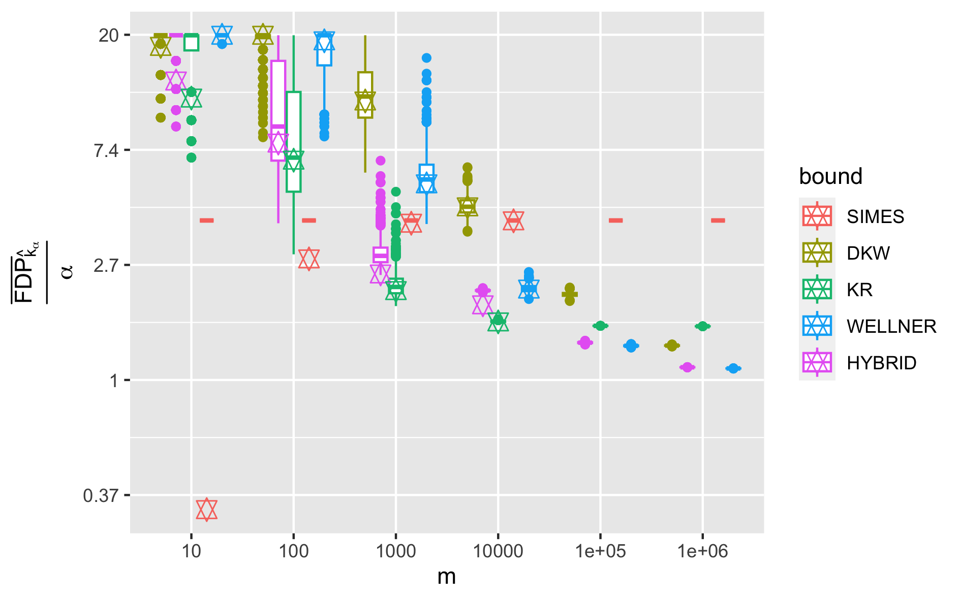
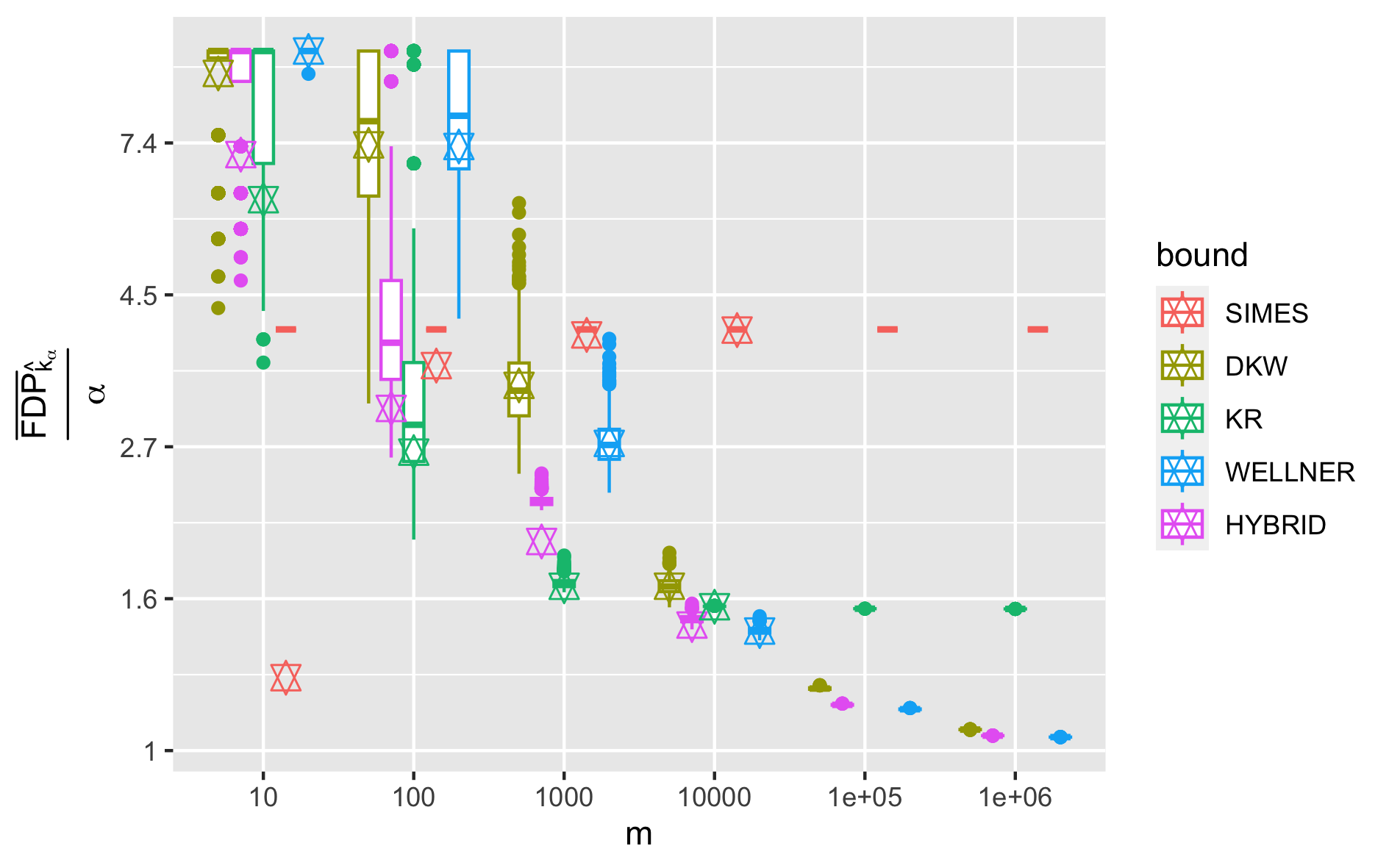
$\alpha=0.15$	$\alpha=0.2$

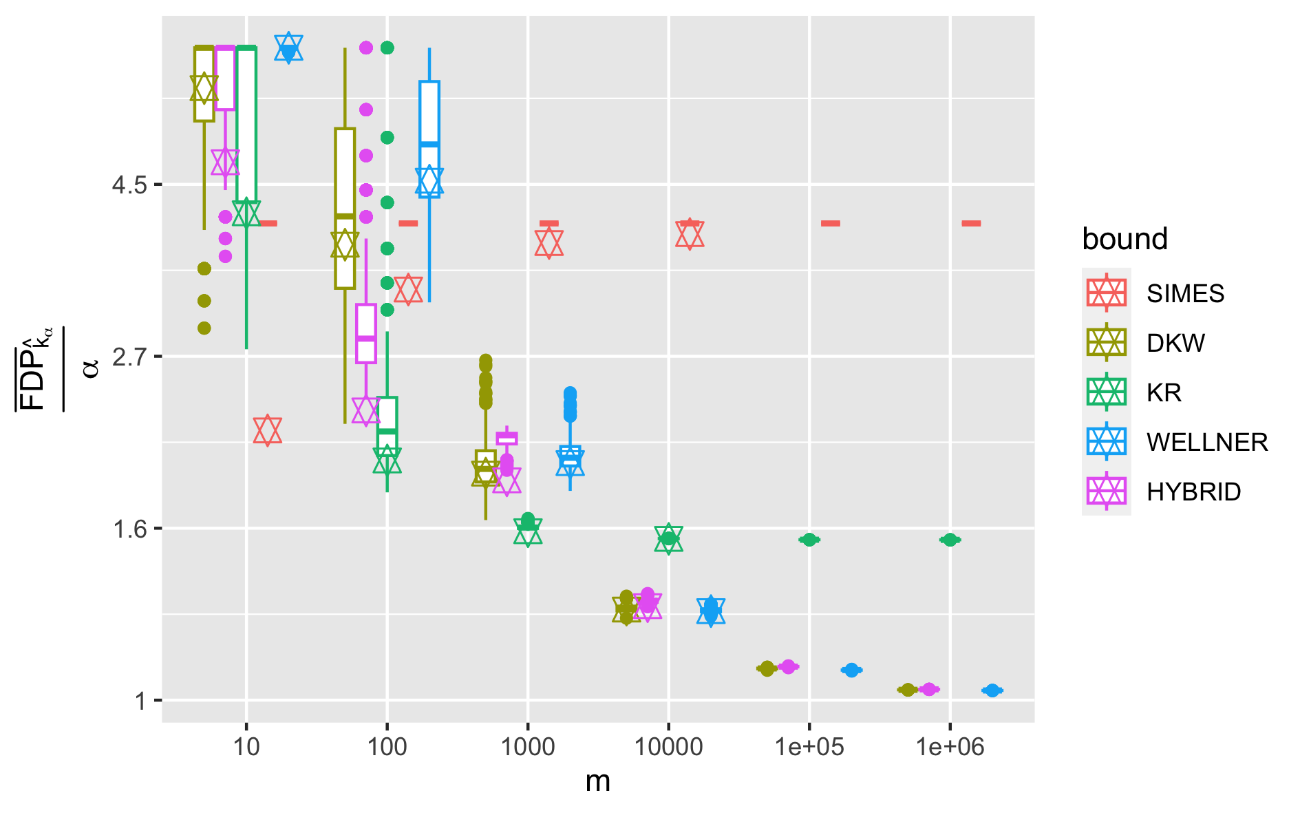
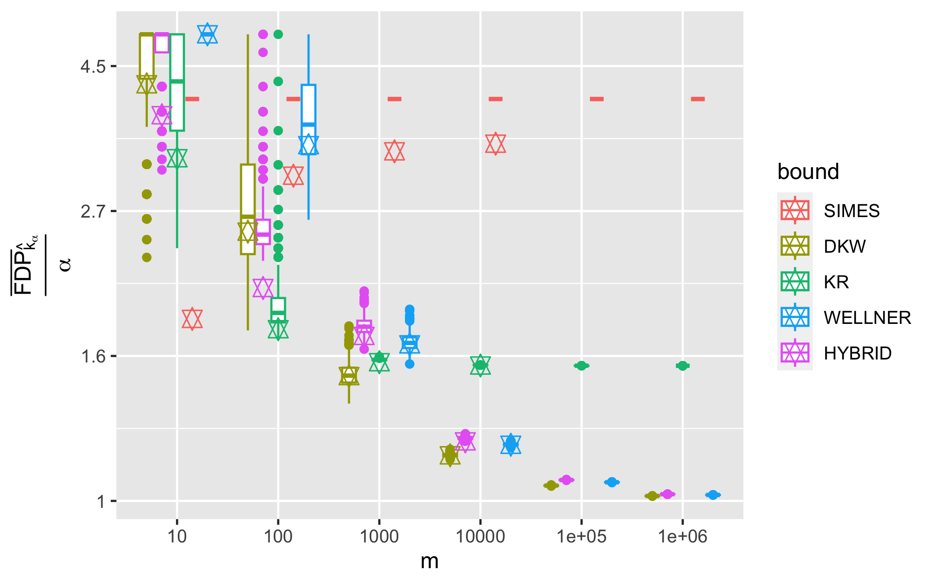
Figure 13: Figure 1 where we have superposed in each case the (median of the) interpolated bounds (star symbols). Top-$k$ dense case ($\pi_{0}=0.5$, $\mu=1.5$).

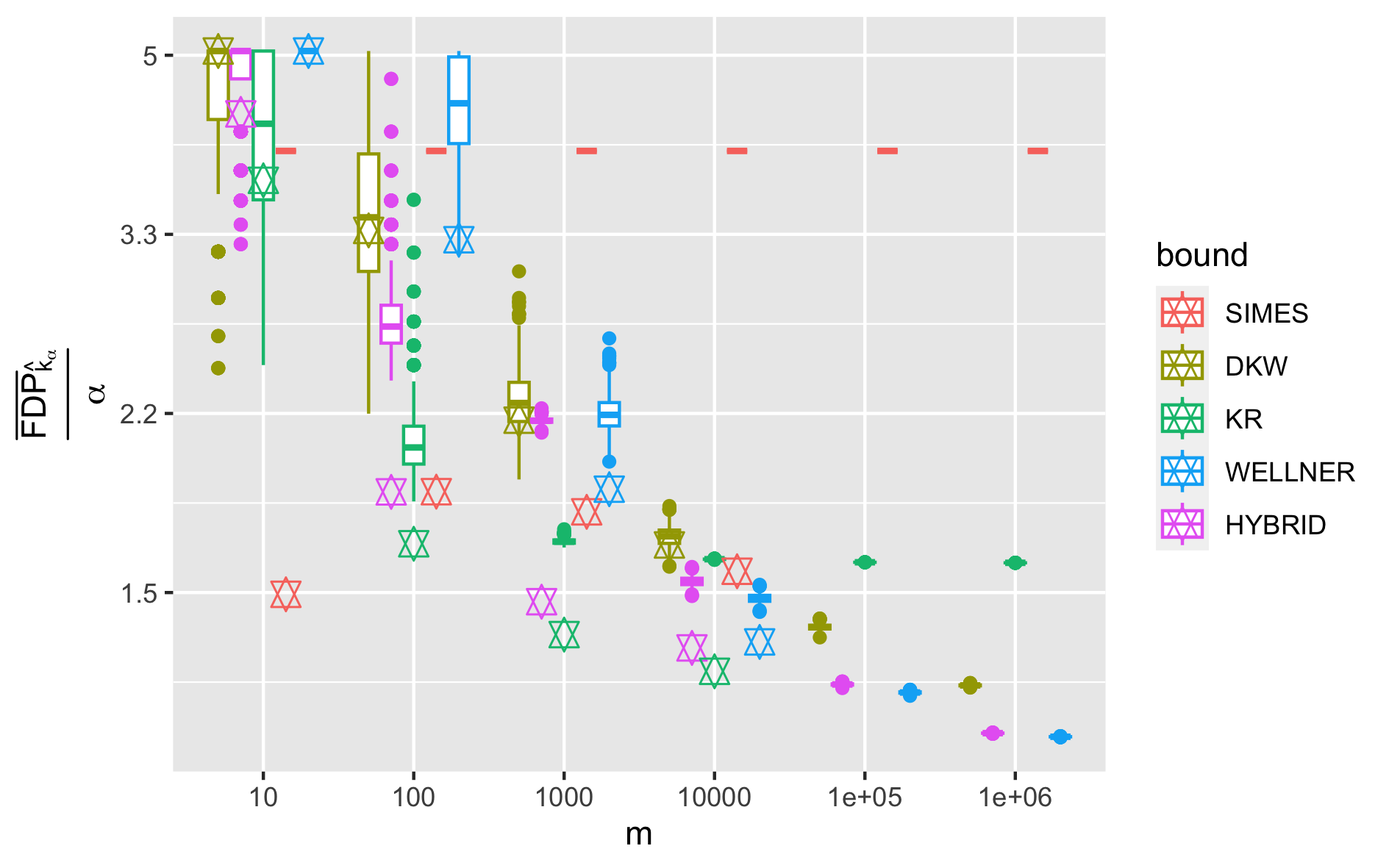
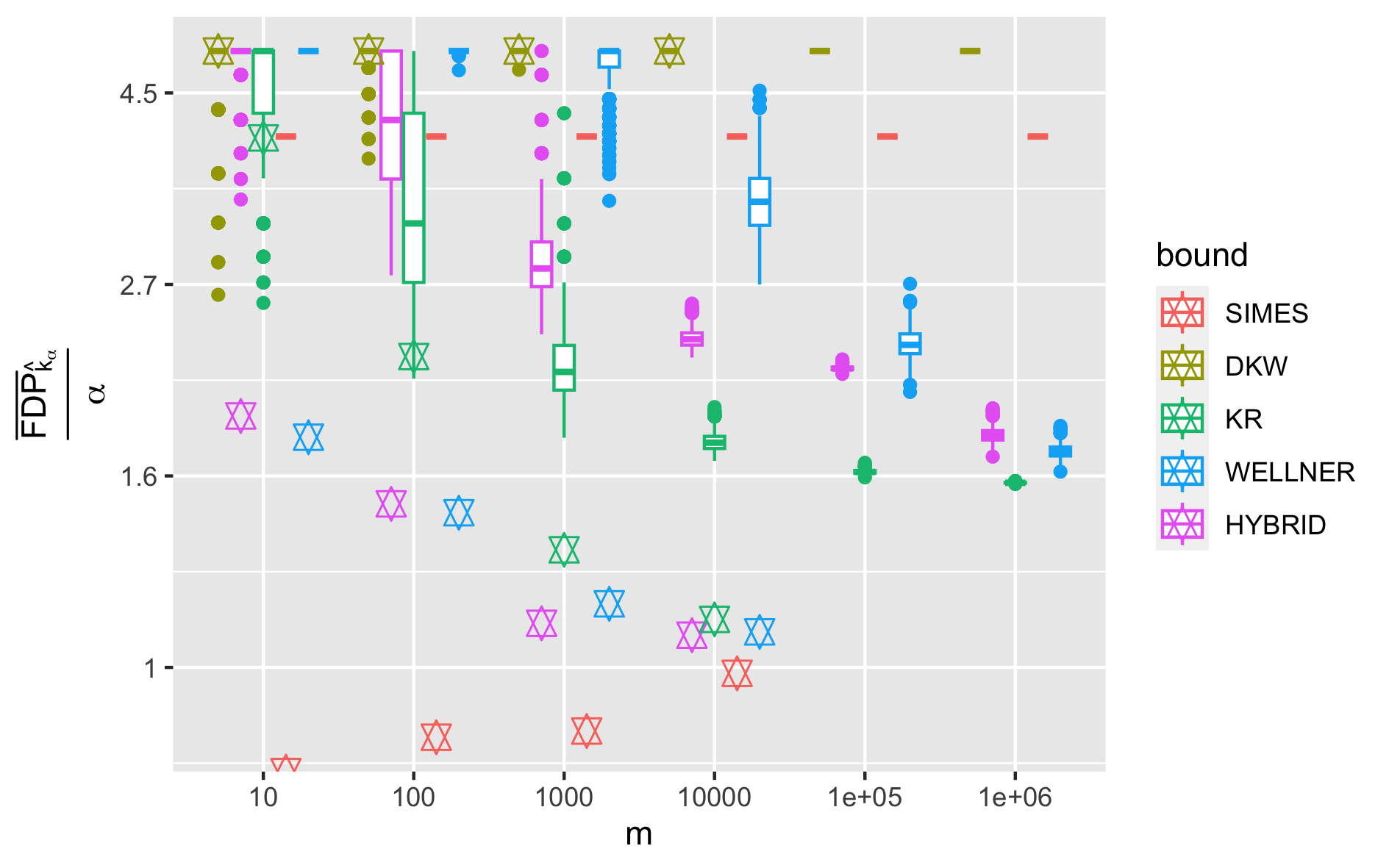
Figure 14: Figure 2 where we have superposed in each case the (median of the) interpolated bounds (star symbols). Top-$k$ sparse case $\pi_{0}=1-0.5m^{-0.25}$, $\mu=\sqrt{2\log m}$ (left) $\pi_{0}=1-0.5m^{-0.55}$, $\mu=$10 (right), $\alpha=0.2$.

Non adaptive	Adaptive

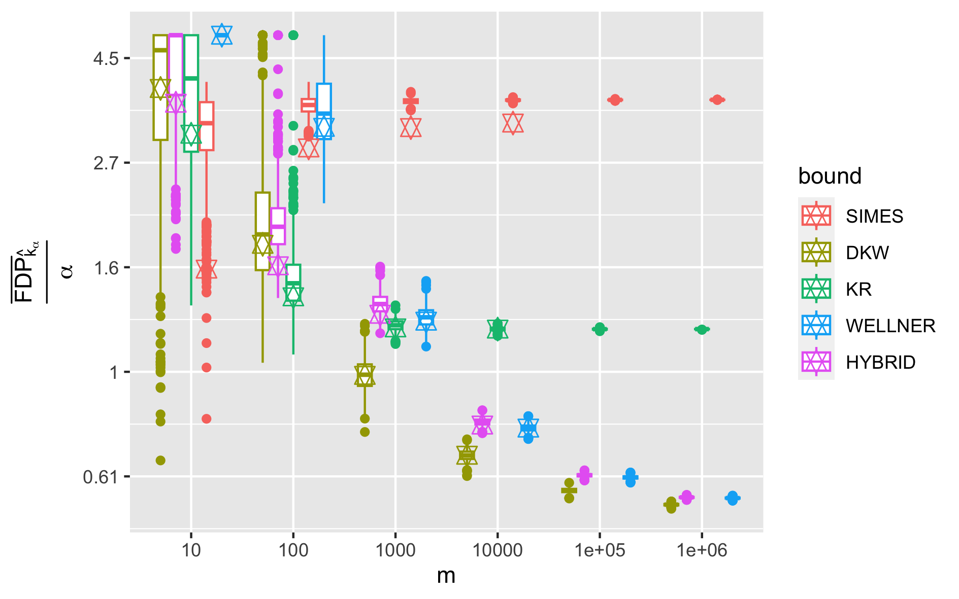
Figure 15: Figure 3 where we have superposed in each case the (median of the) interpolated bounds (star symbols). Top-$k$ dense case with nonadaptive bounds (left) and adaptive bounds (right) ($\pi_{0}=0.5$, $\alpha=0.2$).

$\alpha=0.05$	$\alpha=0.1$
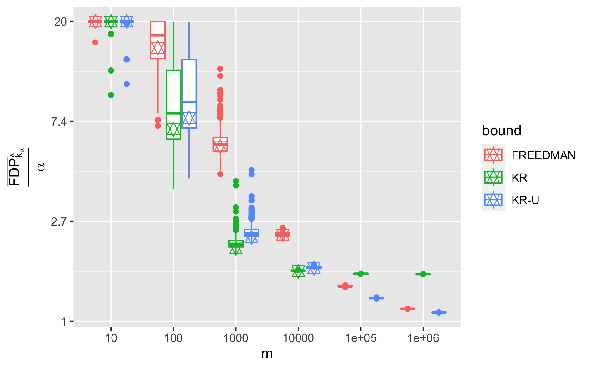
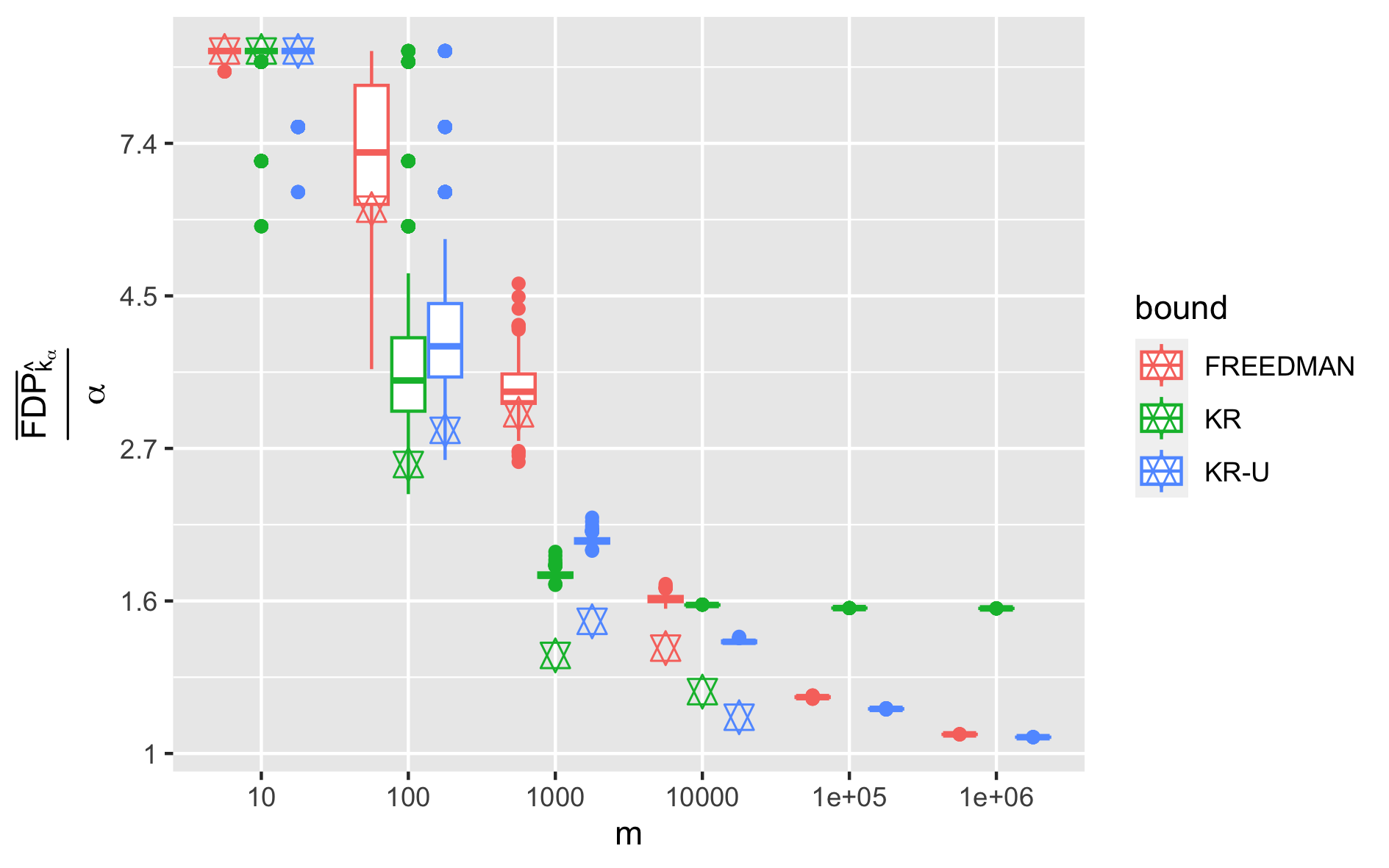
$\alpha=0.15$	$\alpha=0.2$

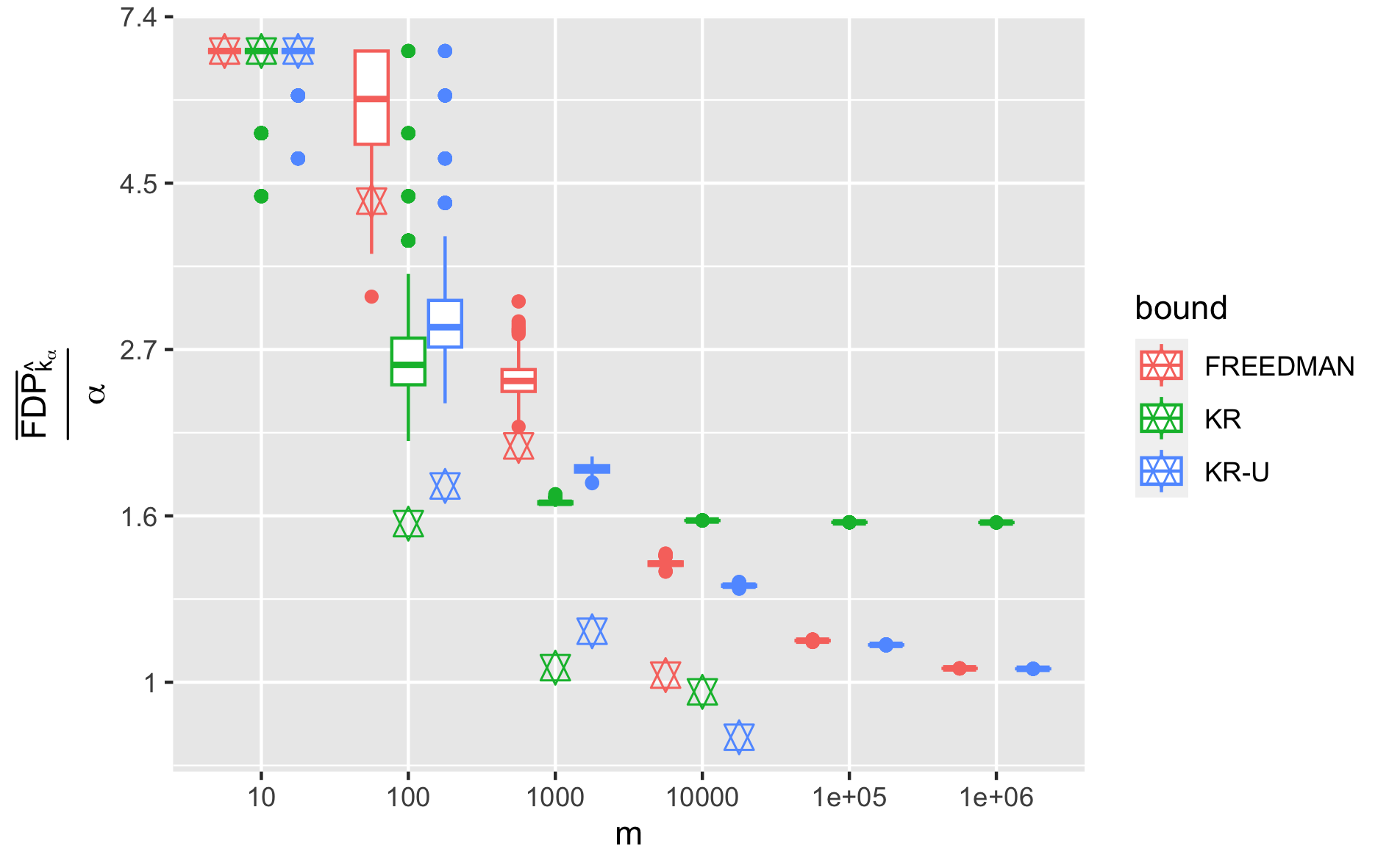
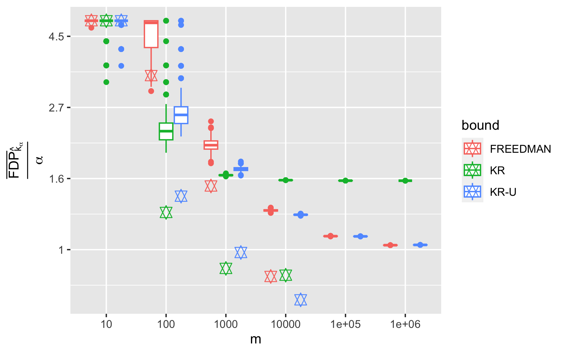
Figure 16: Figure 5 where we have superposed in each case the (median of the) interpolated bounds (star symbols). Preordered dense ($\beta=0$) LF setting with LF procedure ($s=0.1\alpha$, $\lambda=0.5$).

$\alpha=0.05$	$\alpha=0.1$
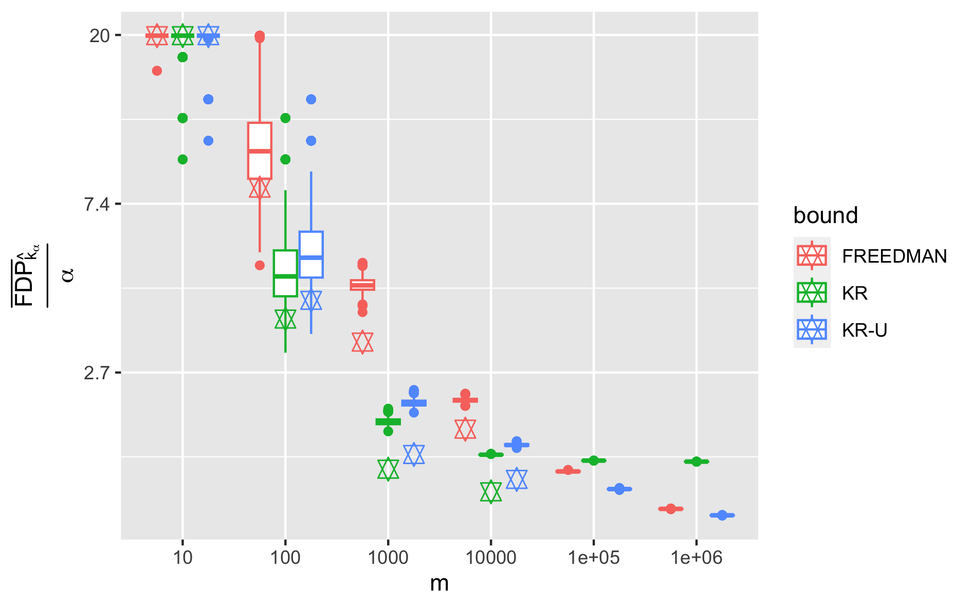
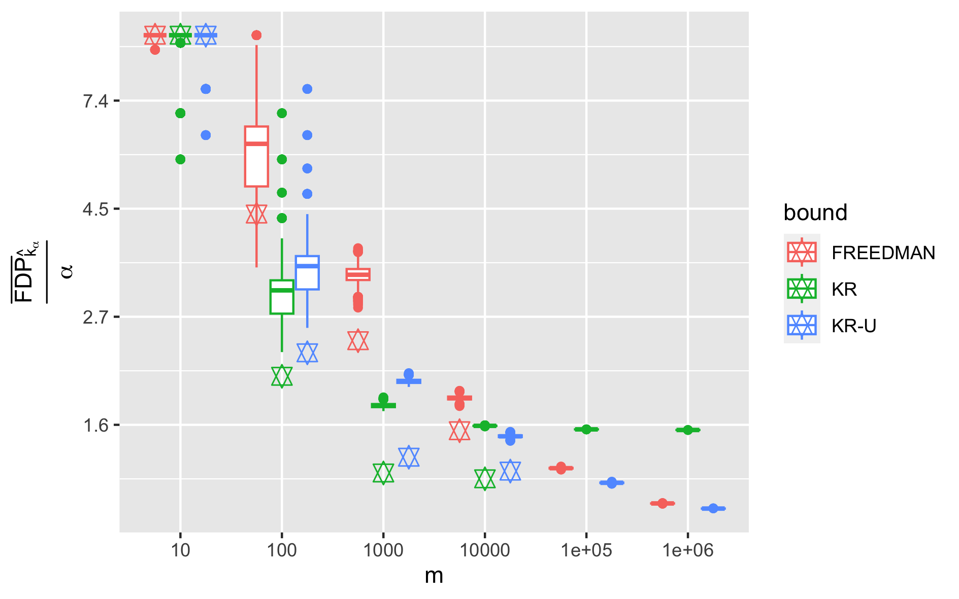
$\alpha=0.15$	$\alpha=0.2$

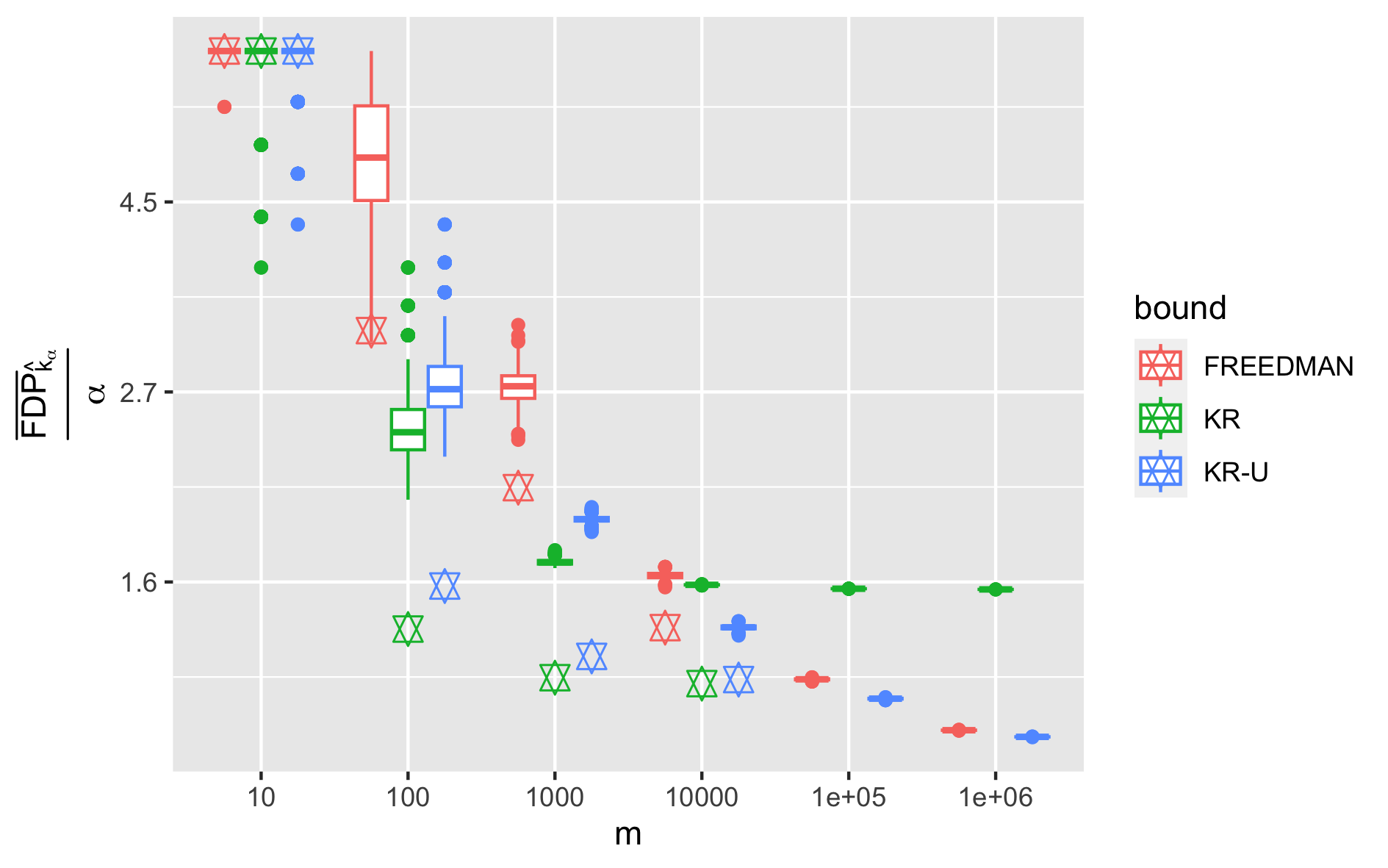
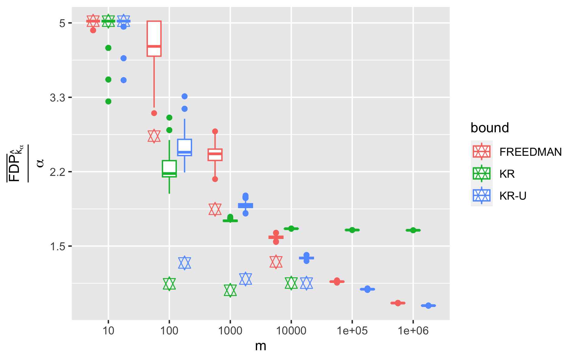
Figure 17: Figure 6 where we have superposed in each case the (median of the) interpolated bounds (star symbols). Preordered sparse ($\beta=0.25$) LF setting with LF procedure ($s=0.1\alpha$, $\lambda=0.5$).

$\alpha=0.15$	$\alpha=0.2$

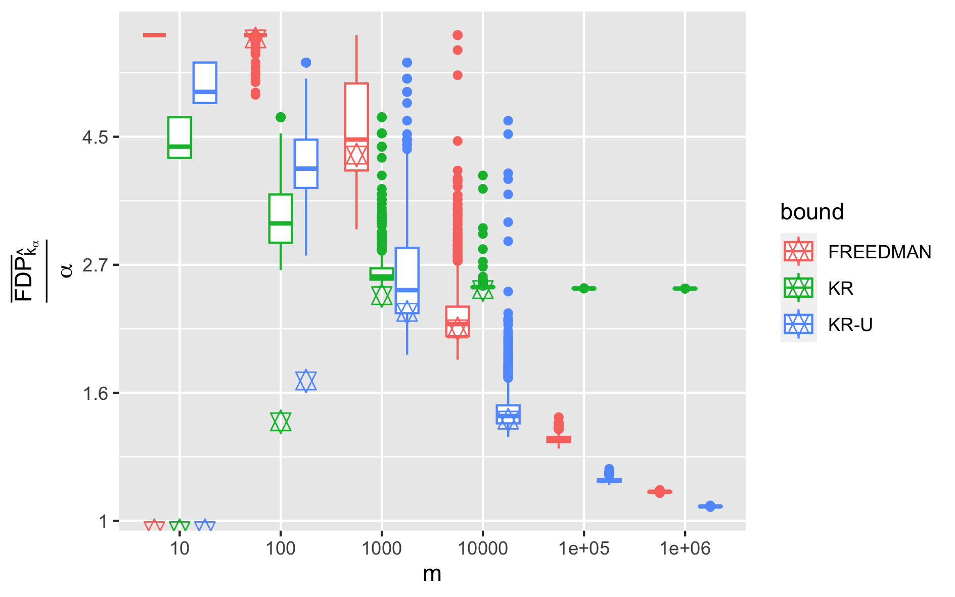
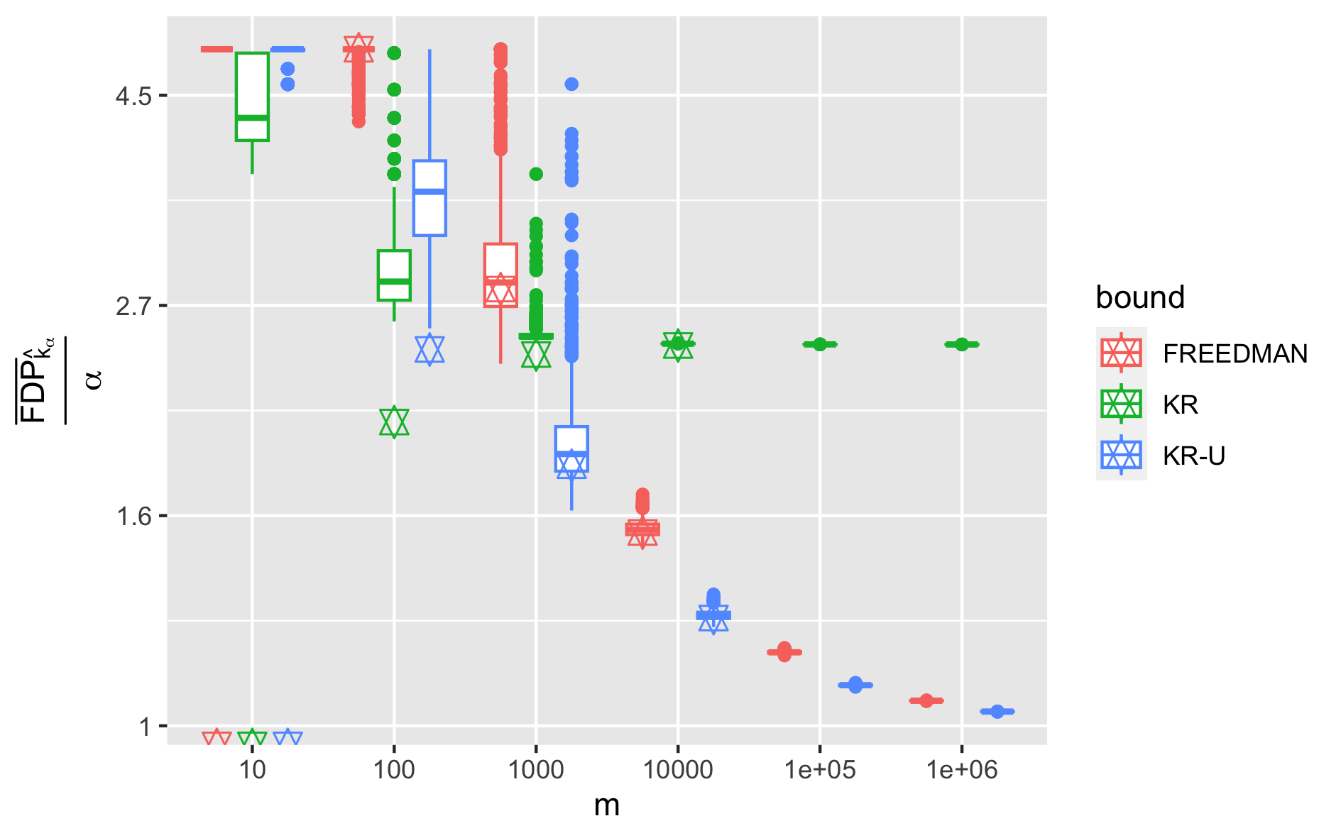
Figure 18: Figure 7 where we have superposed in each case the (median of the) interpolated bounds (star symbols). Pre-ordered dense ($\beta=0$) knockoff setting with BC procedure (i.e., LF procedure with $s=\lambda=0.5$).

$\alpha=0.15$	$\alpha=0.2$

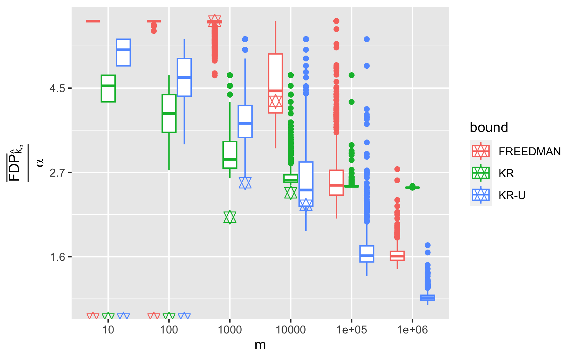
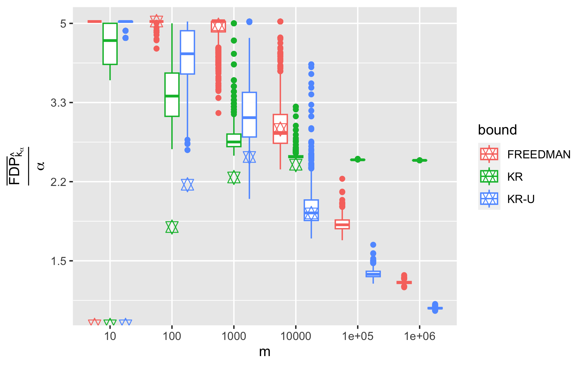
Figure 19: Figure 8 where we have superposed in each case the (median of the) interpolated bounds (star symbols). Pre-ordered sparse ($\beta=0.25$) knockoff setting with BC procedure (i.e., LF procedure with $s=\lambda=0.5$).

References

- Abraham et al., (2021) Abraham, K., Castillo, I., and Roquain, E. (2021). Sharp multiple testing boundary for sparse sequences. arXiv preprint arXiv:2109.13601.
- (2) Aharoni, E. and Rosset, S. (2014a). Generalized -investing: definitions, optimality results and application to public databases. Journal of the Royal Statistical Society: Series B: Statistical Methodology, pages 771–794.
- (3) Aharoni, E. and Rosset, S. (2014b). Generalized alpha-investing: definitions, optimality results and application to public databases. Journal of the Royal Statistical Society. Series B (Statistical Methodology), 76(4):771–794.
- Barber and Candès, (2015) Barber, R. F. and Candès, E. J. (2015). Controlling the false discovery rate via knockoffs. The Annals of Statistics, 43(5):2055–2085.
- Benjamini and Hochberg, (1995) Benjamini, Y. and Hochberg, Y. (1995). Controlling the false discovery rate: A practical and powerful approach to multiple testing. Journal of the Royal Statistical Society. Series B, 57(1):289–300.
- Blanchard et al., (2020) Blanchard, G., Neuvial, P., and Roquain, E. (2020). Post hoc confidence bounds on false positives using reference families. The Annals of Statistics, 48(3):1281–1303.
- Bogdan et al., (2011) Bogdan, M., Chakrabarti, A., Frommlet, F., and Ghosh, J. K. (2011). Asymptotic bayes-optimality under sparsity of some multiple testing procedures. The Annals of Statistics, 39(3):1551–1579.
- Candès et al., (2018) Candès, E., Fan, Y., Janson, L., and Lv, J. (2018). Panning for gold: ‘model-x’ knockoffs for high dimensional controlled variable selection. Journal of the Royal Statistical Society: Series B (Statistical Methodology), 80(3):551–577.
- Cui et al., (2021) Cui, X., Dickhaus, T., Ding, Y., and Hsu, J. C. (2021). Handbook of multiple comparisons. CRC Press.
- Dümbgen and Wellner, (2023) Dümbgen, L. and Wellner, J. A. (2023). A new approach to tests and confidence bands for distribution functions. The Annals of Statistics, 51(1):260–289.
- Durand et al., (2020) Durand, G., Blanchard, G., Neuvial, P., and Roquain, E. (2020). Post hoc false positive control for structured hypotheses. Scandinavian journal of Statistics, 47(4):1114–1148.
- Foster and Stine, (2008) Foster, D. P. and Stine, R. A. (2008). Alpha-investing: a procedure for sequential control of expected false discoveries. Journal of the Royal Statistical Society: Series B (Statistical Methodology), 70(2):429–444.
- Freedman, (1975) Freedman, D. A. (1975). On tail probabilities for martingales. The Annals of Probability, pages 100–118.
- Genovese and Wasserman, (2004) Genovese, C. and Wasserman, L. (2004). A stochastic process approach to false discovery control. The annals of statistics, 32(3):1035–1061.
- Genovese and Wasserman, (2006) Genovese, C. R. and Wasserman, L. (2006). Exceedance control of the false discovery proportion. Journal of the American Statistical Association, 101(476):1408–1417.
- Goeman et al., (2021) Goeman, J. J., Hemerik, J., and Solari, A. (2021). Only closed testing procedures are admissible for controlling false discovery proportions. The Annals of Statistics, 49(2):1218 – 1238.
- Goeman et al., (2019) Goeman, J. J., Meijer, R. J., Krebs, T. J., and Solari, A. (2019). Simultaneous control of all false discovery proportions in large-scale multiple hypothesis testing. Biometrika, 106(4):841–856.
- Goeman and Solari, (2011) Goeman, J. J. and Solari, A. (2011). Multiple testing for exploratory research. Statistical Science, 26(4):584–597.
- Hemerik et al., (2019) Hemerik, J., Solari, A., and Goeman, J. J. (2019). Permutation-based simultaneous confidence bounds for the false discovery proportion. Biometrika, 106(3):635–649.
- Howard et al., (2021) Howard, S. R., Ramdas, A., McAuliffe, J., and Sekhon, J. (2021). Time-uniform, nonparametric, nonasymptotic confidence sequences. The Annals of Statistics, 49(2):1055 – 1080.
- Jamieson et al., (2014) Jamieson, K., Malloy, M., Nowak, R., and Bubeck, S. (2014). lil’UCB: An optimal exploration algorithm for multi-armed bandits. In Conference on Learning Theory, pages 423–439. PMLR.
- Javanmard and Montanari, (2018) Javanmard, A. and Montanari, A. (2018). Online rules for control of false discovery rate and false discovery exceedance. The Annals of statistics, 46(2):526–554.
- Katsevich and Ramdas, (2020) Katsevich, E. and Ramdas, A. (2020). Simultaneous high-probability bounds on the false discovery proportion in structured, regression and online settings. The Annals of Statistics, 48(6):3465–3487.
- Lei and Fithian, (2016) Lei, L. and Fithian, W. (2016). Power of ordered hypothesis testing. In International conference on machine learning, pages 2924–2932. PMLR.
- Li and Barber, (2017) Li, A. and Barber, R. F. (2017). Accumulation tests for fdr control in ordered hypothesis testing. Journal of the American Statistical Association, 112(518):837–849.
- Li et al., (2022) Li, J., Maathuis, M. H., and Goeman, J. J. (2022). Simultaneous false discovery proportion bounds via knockoffs and closed testing. arXiv preprint arXiv:2212.12822.
- Massart, (1990) Massart, P. (1990). The tight constant in the Dvoretzky-Kiefer-Wolfowitz inequality. Ann. Probab., 18(3):1269–1283.
- Meinshausen, (2006) Meinshausen, N. (2006). False discovery control for multiple tests of association under general dependence. Scandinavian Journal of Statistics, 33(2):227–237.
- Meinshausen and Bühlmann, (2005) Meinshausen, N. and Bühlmann, P. (2005). Lower bounds for the number of false null hypotheses for multiple testing of associations under general dependence structures. Biometrika, 92(4):893–907.
- Meinshausen and Rice, (2006) Meinshausen, N. and Rice, J. (2006). Estimating the proportion of false null hypotheses among a large number of independently tested hypotheses. The Annals of Statistics, 34(1):373 – 393.
- Muñoz-Fuentes et al., (2018) Muñoz-Fuentes, V., Cacheiro, P., Meehan, T. F., Aguilar-Pimentel, J. A., Brown, S. D. M., Flenniken, A. M., Flicek, P., Galli, A., Mashhadi, H. H., Hrabě De Angelis, M., Kim, J. K., Lloyd, K. C. K., McKerlie, C., Morgan, H., Murray, S. A., Nutter, L. M. J., Reilly, P. T., Seavitt, J. R., Seong, J. K., Simon, M., Wardle-Jones, H., Mallon, A.-M., Smedley, D., and Parkinson, H. E. (2018). The International Mouse Phenotyping Consortium (IMPC): a functional catalogue of the mammalian genome that informs conservation the IMPC consortium. Conservation Genetics, 3(4):995–1005.
- Neuvial, (2008) Neuvial, P. (2008). Asymptotic properties of false discovery rate controlling procedures under independence. Electron. J. Statist., 2:1065–1110.
- Neuvial, (2013) Neuvial, P. (2013). Asymptotic results on adaptive false discovery rate controlling procedures based on kernel estimators. Journal of Machine Learning Research, 14:1423–1459.
- Neuvial and Roquain, (2012) Neuvial, P. and Roquain, E. (2012). On false discovery rate thresholding for classification under sparsity. The Annals of Statistics, 40(5):2572–2600.
- Perrot-Dockès et al., (2021) Perrot-Dockès, M., Blanchard, G., Neuvial, P., and Roquain, E. (2021). Post hoc false discovery proportion inference under a hidden markov model. arXiv preprint arXiv:2105.00288.
- Ramdas et al., (2017) Ramdas, A., Yang, F., Wainwright, M. J., and Jordan, M. I. (2017). Online control of the false discovery rate with decaying memory. In Guyon, I., Luxburg, U. V., Bengio, S., Wallach, H., Fergus, R., Vishwanathan, S., and Garnett, R., editors, Advances in Neural Information Processing Systems, volume 30. Curran Associates, Inc.
- Robbins, (1954) Robbins, H. (1954). A one-sided confidence interval for an unknown distribution function. Annals of Mathematical Statistics, 25(2):409–409.
- Robertson et al., (2022) Robertson, D. S., Wason, J., and Ramdas, A. (2022). Online multiple hypothesis testing for reproducible research. arXiv preprint arXiv:2208.11418.
- Shorack and Wellner, (2009) Shorack, G. R. and Wellner, J. A. (2009). Empirical processes with applications to statistics. SIAM.
- Storey, (2002) Storey, J. D. (2002). A direct approach to false discovery rates. Journal of the Royal Statistical Society: Series B (Statistical Methodology), 64(3):479–498.
- Vesely et al., (2021) Vesely, A., Finos, L., and Goeman, J. J. (2021). Permutation-based true discovery guarantee by sum tests. arXiv preprint arXiv:2102.11759.