simmr: A package for fitting Stable Isotope Mixing Models in R

Emma Govan, Andrew L Jackson, Richard Inger, Stuart Bearhop, Andrew C Parnell simmr: A package for fitting Stable Isotope Mixing Models in R A package for SIMMs in R We introduce an R package for fitting Stable Isotope Mixing Models (SIMMs) via both Markov chain Monte Carlo and Variational Bayes. The package is mainly used for estimating dietary contributions from food sources taken via measurements of stable isotope ratios from animals. It can also be used to estimate proportional contributions of a mixture from known sources, for example apportionment of river sediment, amongst many other use cases. The package contains a simple structure which allows non-expert users to interface with the package, with most of the computational complexity hidden behind the main fitting functions. In this paper we detail the background to these functions and provide case studies on how the package should be used. Further examples are available in the online package vignettes. ecological modeling, stable isotope mixing models (SIMMs), R, Markov chain Monte Carlo, Variational Bayes ecological modeling, stable isotope mixing models (SIMMs), R, MArkov chain Monte Carlo, Variational Bayes Emma Govan
Hamilton Institute
Insight Centre for Data Analytics
Maynooth University
Maynooth
Ireland
E-mail:

1 Introduction

Stable Isotope Mixing Models (SIMMs) are a useful tool for ecologists, especially in the reconstruction of animal diets (deniro1978influence). Starting from stable isotope measurements of animal tissues and their food sources, mixing models allow for estimation of the proportional composition of their food sources in their diet (mckechnie2004stable). Stable isotope ratios represent the difference in relative abundance of non-radiogenic, stable isotopes expressed as the ratio of an isotope’s "heavy" form of an element versus a "light" form relative to an internationally accepted standard. These stable isotope ratios can vary geo-spatially and across the different levels of food webs (hobson1999tracing). Isotopic data can be obtained relatively easily and allow for many different aspects of diet to be analysed, for example across timescales or locations, depending on the sampled tissues. Typical ecological applications include quantifying animal diets (peterson1987stable), and estimating the origins of migratory animals (hobson1999tracing). Whilst isotope ratios were the original data used for these models, other data are used (see later discussion on end member analysis), so these data are referred to more generically as tracers in the simmr package. Similarly, the consumers (usually animals) are referred to more generically as mixtures.

SIMMs require data from both the mixtures being studied as well as all of their sources (for example, the foods they are consuming when we are looking at animal diets). When studying animals, the data can be obtained via tissue samples, such as blood or feathers, depending on the time-frame being studied. For example, isotopes from food are assimilated quickly into tissues with rapid turnover rates such as blood and so this provides a relatively recent estimate of their diet (TieszenTissue1983); metabolically inactive tissues such as feathers or hair preserve an isotopic record of the diet at the time they were grown (inger2008applications), and samples from otoliths may provide an overview of the diet of a fish over their lifetime (RadtkeOtolith1996) with successive layers of the tissue being a record of diet through time. Typically, empiricists will make an assumption that a consumer (the mixture) is at equilibrium with its food sources in order to estimate the dietary proportions at a fixed time point. Similarly, users of mixing models are required to assume that all of the potential food sources have been sampled and included in the model (phillips2014best). A final parameter that needs to be known or estimated is the trophic discrimination factor (or trophic enrichment factor), which describes the change in isotope ratio between the diet and assimilation into consumer proteins. This can be estimated from captive studies of the same species, literature searches of closely related or functionally similar species or in some cases using the software package SIDER (healy2018sider).

Our paper covers the maths behind the models used for SIMM analysis in the R (rref) package simmr. We demonstrate how to use the package with an example of Brent Geese data from inger2006temporal. The package aims to provide a set of powerful tools, but with a simple to use interface which allows beginners to run models sensibly whilst also allowing advanced users full access to all posterior quantities of the back-end Bayesian model.

The basic mathematical equation for a statistical SIMM is:

$$y=\sum_{k=1}^{K}p_{k}s_{k}+\epsilon$$

where $y$ is the mixture value, $p_{k}$ are the proportions associated with source $k$ (of $K$ total sources), $s_{k}$ is the source tracer value for source $k$, and $\epsilon$ is a residual term. In this over-simplification of the model (see Section 4 for a more complete version), $s_{k}$ is an individual level random effect with a given mean and standard deviation, $s_{k}\sim N(\mu_{sk},\sigma^{2}_{sk})$, and the key task of the model is to estimate the $p_{k}$ proportions. We call $y$ the mixture value for each individual, but they can also be referred to as the consumer value or end member value in the literature.

There are now a number of software tools for fitting SIMMs, which are discussed in detail in Section 3. Whilst these models are mainly used to study the proportional contribution that different foods make up in an animal’s diet, SIMMs can also be used in a wide range of different scenarios. These include the study of a Late Pleistocene bear (mychajliw2020biogeographic), which confirmed its trophic position is similar to other bears of the same species, and the study of crop usage in Iron Age settlements (styring2022proof). We expand on this set of examples below.

Models mathematically identical to SIMMs are also used in many other areas. These are often known as ‘end member analysis’, ‘mass balance analysis’, or ‘source apportionment’. hopke1991receptor is an early review of source apportionment models. It uses linear equations and a least-squares method for running these models. henry1997history explores different methods of running these models, such as a geometrical approach. Prior knowledge is then incorporated in billheimer2001compositional, which is Bayesian based, and a non-additive error structure is also adopted. park2001multivariate incorporates temporal dependence and adopts a MCMC approach to estimate parameters. lingwall2008dirichlet uses a Dirichlet prior distribution to allow flexible specification of prior information. The European Union has published several guides on use of source apportionment with receptor models in studies (e.g. european2019; mircea2020european).

End member analysis is generally employed by geologists and is used to estimate how different water sources contribute to a mixture. Examples include soulsby2003identifying, which employs MCMC methods to study runoff sources during storms in Scotland. brewer2011source employs MCMC methods to study runoff sources. Their model allows for consideration of random effects, such as comparison across years. palmer2008bayesian operates using MCMC and estimates the proportion that different water sources have contributed to sediment samples. liu2020quantification adopts a maximum likelihood method to estimate water sources. Their method employs a multivariate statistical approach to allow for uncertainty in the concentration of end-members, or sources. The end-members contributing to the mixture are first identified and then the proportion that each contributes is calculated. tao2021endmember proposes a maximum distance analysis method that estimates both the number and spectral signatures of end-members, which means that it is not essential to know the number and identity of end-members in advance in order for a model to be run.

Another term commonly employed for SIMMs is that of mass balance modelling. The term is often used for apportioning sources of pollution. christensen2004chemical evaluates several of these methods, for example weighted least squares and the method of moments. In campodonico2019chemical a log-ratio technique is used to analyse how elements move during chemical weathering. cooper2014sensitivity uses SIMM-related modelling to study suspended particulate matter. They look at several different models and provide comparison and advice on choosing an appropriate model. Code is provided for one of their models.

Our package simmr implements mixing models via both Markov Chain Monte Carlo (MCMC) algorithms and faster Fixed Form Variational Bayes (FFVB). It is not designed to be more fully featured than other R packages that fit SIMMs, rather we aim for a simple unified data structure that enables both non-experts and advanced users to access the tools they need. FFVB is introduced as a foundation to enable much faster fitting of SIMMS, where MCMC can be prohibitively slow. The data structure needed for running SIMMs can be complex, using multiple different data frames of different dimensions, but simmr makes it easy to read in the data and subsequently create plots and model output. We use a Snake case naming convention for consistency and follow the ‘tidyverse’ (tidyverseref) style guide. We aim to keep the number of functions to a minimum and use S3 classes for access to summary and plot commands. Our visualisations are carefully selected for style and colour choices, and easily produced through built-in functions using ggplot2 (ggplot2ref). We aim to make all our functions easily extendable so that advanced users can create more complicated outputs.

SIMMs are widely used and applicable in many areas. Thus the R packages for running them are frequently downloaded and have received thousands of citations between them. Figure 1 shows the citation rates of the main papers used for SIMMs and the number of downloads of the associated R packages.

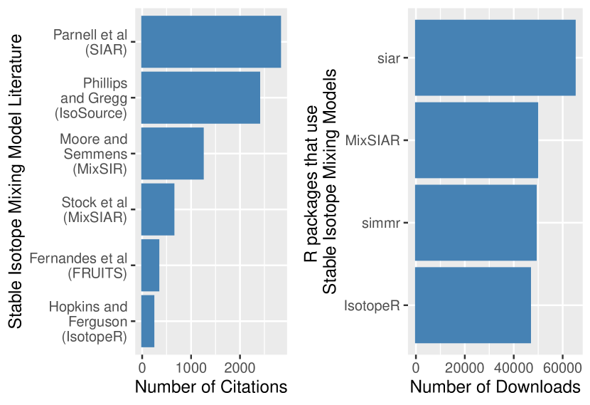
Figure 1: Barplot on the left showing the number of downloads that packages using stable isotope mixing models have obtained (download numbers obtained via the cranlogs package (cranlogsref)) and barplot on the right showing the number of citations papers describing SIMMs software have received on Google Scholar (figures correct as of 9th June 2023).

2 A short guide to fitting SIMMs using simmr

The first step in using simmr is to install and load the package: R> install.packages("simmr") R> library(simmr) simmr requires the user to provide mixture data ($y$), source means ($\mu_{sk}$), and source standard deviations ($\sigma_{sk}$). Other variables can be included as described in Section 4. The data is read into R using the simmr_load function. We will use an artificially generated dataset for illustration: R> y = data.frame(iso1 = c(4, 4.5, 5, 7, 6, 2, 3, 3.5, 5.5, 6.5)) R> mu_s = matrix(c(-10, 0, 10), ncol = 1, nrow = 3) R> sigma_s = matrix(c(1, 1, 1), ncol = 1, nrow = 3) R> s_names = c("A", "B", "C") These artificially simple data have measurements of one isotope ratio, named ‘iso1‘ and three food sources, labelled A, B, and C. Loading the data into simmr creates an object of class simmr_in: R> simmr_in_1 = simmr_load( + mixtures = y, + source_names = s_names, + source_means = mu_s, + source_sds = sigma_s) We recommend that the user plot these data on an ‘iso-space’ plot before running any model. The iso-space plot shows the isotope(s) ratio on the x (and potentially y) axes. In this case, with one isotope, we need to check that the mixture values lie between the two most extreme values of the food sources on the iso-space plot for the mathematical model to give a reasonable fit to the data. With two isotopes its important to check that the mixture lies within the polygon that can be drawn by joining the food sources with straight lines. The shape created by joining the food sources is referred to as the mixing polygon. The iso-space plot can be generated by running the code: R> plot(simmr_in_1)

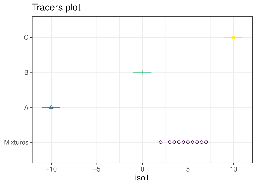
Figure 2: Simple iso-space plot produced by simmr. The isotope ratios are presented on the x-axis. A, B, and C represent different food sources (with error bars included) and the purple dots represent the mixture values.

Figure 2 shows the isospace plot for this simple example, which shows the mixtures lie within the values of the most extreme food sources.The SIMM can then be fitted via MCMC using the simmr_mcmc function, which produces an object of class simmer_output and mcmc:

R> simmr_out_1 = simmr_mcmc(simmr_in_1)

When running simmr_mcmc the first step after running the model is to check convergence. This can be performed by running the following code: R> summary(simmr_out_1, type = "diagnostics") Summary for 1 Gelman diagnostics - these values should all be close to 1. If not, try a longer run of simmr_mcmc. deviance A B C sd[iso1] 1.00 1.00 1.00 1.01 1.00 The values in the diagnostics should all be close to 1.

simmr produces both textual and graphical summaries of the model run. Starting with the textual summaries, we can get tables of the means, standard deviations and credible intervals (the Bayesian equivalent of a confidence interval) with: R> summary(simmr_out_1, type = "statistics") Summary for 1 mean sd deviance 39.269 2.539 A 0.147 0.065 B 0.243 0.131 C 0.610 0.079 sd[iso1] 1.717 0.602

This summary provides the mean and standard deviation estimates for the proportion of each food (A, B, and C) that these individuals are eating. It also provides an estimate of the marginal residual error of the isotope ratio (iso1 in this case). Here we can see food C is estimated to make up approximately 61% of these animals’ diet. This finding matches the isospace plot where the consumer isotope ratios are closest to the values for source C.

simmr has built-in functions to allow for visualisation of the results of these models once they have been run. There are multiple options for plotting the output, but perhaps the most useful is the matrix plot:

R> plot(simmr_out_1, type = "matrix")

Figure 3 shows histograms of the posterior distribution for the dietary proportions of each source on the diagonal, contour plots of the posterior relationship between the dietary proportions of each food source on the upper-right portion of the plot, and the posterior correlation between the sources on the lower-left portion of the plot. Large negative correlations indicate that the model cannot discern between the two sources; for example they may lie close together in iso-space. Large positive correlations are also possible when there are multiple competing sources. In general, high correlations (negative or positive) are indicative of the model being unable to determine which food sources are being consumed, though the marginal standard deviations can still be narrow. In this case the large negative correlations exist because there is only a single isotope and the model cannot discern, for example, which of sources A and B are pulling the mixture values to the left of source C.

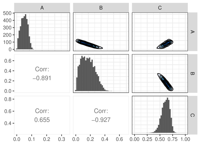
Figure 3: Matrix plot generated from Markov chain Monte Carlo run on Stable Isotope Mixing Model with 1 isotope. Histograms are presented along the diagonal showing the estimated proportion of each food source (A, B, and C) consumed by the individual. The upper-right section shows contour plots. The lower-left section gives correlation values.

3 Other software for fitting stable isotope mixing models

There have been many different software tools developed for the study of SIMMs. Table 1 gives a summary of these tools with a short description. The methods behind these tools includes both Frequentist and Bayesian approaches, and a variety of different fitting techniques. For reference, we provide code to fit our case study data (Section 6) using these packages at https://github.com/emmagovan/simmr_paper_SIMM_package_scripts.

Package	Language	Reference	Description
Isosource	Visual Basic	phillips2003source	Calculates all possible source combinations and returns feasible solutions
MixSIR	Matlab	moore2008incorporating	Bayesian - Uses a sampling-importance-resampling algorithm
siar	R	parnell2010source	Bayesian - uses Markov chain Monte Carlo (MCMC) for its fitting algorithm
FRUITS	Visual Basic	fruits	Bayesian - allows for consideration of dietary routing. Operates based on Markov chain Monte Carlo simulations.
MixSIAR	R	stock2018analyzing	Bayesian - allows for consideration of fixed and random effects
simmr	R	This paper	Bayesian - can use either MCMC or fixed form variational Bayes (FFVB)

Table 1:

Overview of different software for running Stable Isotope Mixing Models

The first widely available software for fitting SIMMs was IsoSource (phillips2003source), which worked by generating all possible combinations of dietary proportions that would add to give the isotopic value of the individuals being studied, and presenting all possible combinations to the user. The recommendation was to report the distribution of solutions to avoid any misinterpretation of results. IsoSource was implemented in Visual Basic via the IsoSource computer programme. Whilst IsoSource did not account for many of the intricacies of SIMMs, it was based on several previously developed ideas including concentration dependence, which provides the proportion of each element directly in the food source, (IsoConc; phillips2002incorporating) and residual error (IsoError; phillips2001uncertainty).

MixSIR (moore2008incorporating) was later developed and was the first to use a Bayesian framework, based on importance resampling, to estimate dietary proportions. MixSIR works by generating many vectors of possible proportional source contribution and calculating importance weights to determine the posterior distribution. MixSIR is implemented in MATLAB. It allows for several extensions over IsoSource including the ability to account for uncertainty, and incorporation of prior information. See Section 4 for a full description of these terms.

SIAR (parnell2010source) used a Bayesian framework but with Markov chain Monte Carlo (MCMC) as the fitting algorithm. It includes a residual error term and many of the extensions included in MixSIR. The R package is now defunct but maintained on GitHub for backwards compatibility. We have designed simmr to be a replacement for the SIAR software.

The FRUITS model (fruits) further extended the work by allowing the user to account for the concentration of different food fractions within each food source. FRUITS can also account for a diet-to-tissue signal offset which accounts for different tissues containing different ratios of isotopes, which is the same as concentration dependence discussed in Section 4. It also simplifies the incorporation of prior information. FRUITS is implemented in Visual Basic via the FRUITS computer programme.

The most recent and perhaps most powerful R package, MixSIAR (stock2018analyzing), is Bayesian, and allows for consideration of both fixed and random effect covariates on the dietary proportions amongst other extensions. MixSIAR works by creating a custom JAGS (Just Another Gibbs Sampler, plummer2003jags) file for each model run. The package has a number of example data sets included and produces a wide array of output plots and summary statistics. However the model may not be appropriate for novice users and is very slow for complex data sets; which provides the motivation for development of simmr and the incorporation of FFVB.

4 Mathematical background of mixing models

The full model implemented in simmr for fitting a SIMM is:

$$y_{ij}\sim N\left(\frac{\sum_{k=1}^{K}p_{k}q_{jk}(\mu_{s,jk}+\mu_{c,jk})}{\sum_{k=1}^{K}p_{k}q_{jk}},\frac{\sum_{k=1}^{K}p_{k}^{2}q_{jk}^{2}(\sigma_{s,jk}^{2}+\sigma_{c,jk}^{2})}{(\sum_{k=1}^{K}p_{k}q_{jk})^{2}}+\sigma_{j}^{2}\right)$$

where:

• $y_{ij}$ are the mixture values for individual $i$ on tracer $j$,

• $\mu_{s,jk}$ and $\sigma_{s,jk}$ are the mean and standard deviation of the source values for source $k$ on tracer $j$,

• $\mu_{c,jk}$ and $\sigma_{c,jk}$ are the mean and standard deviation of the trophic discrimination factors(TFFs or "corrections") for source $k$ on tracer $j$,

• $q_{jk}$ represents concentration dependence for tracer $j$ on source $k$,

• $p_{k}$ are the proportions of each source $k$ contributing to the mixture value

• $\sigma_{j}$ is the residual standard deviation on tracer $j$.

The values $y$, $\mu_{s,jk}$, $\sigma_{s,jk}$, $q_{jk}$, $\mu_{c,jk}$, and $\sigma_{c,jk}$ are all given to the model as data.

The key extension of this model compared to the simple example given in Section 2 are that the model now includes multiple tracers, and corrects the proportions for Trophic Discrimination Factors (TDFs) and concentration dependence. As outlined above, TDFs account for the differential loss of one isotope over the other during the assimilation of diet into consumer proteins (inger2008applications). Different tissues have different macronutrient compositions so TDFs can vary by tissue within a single consumer. Likewise different dietary items contain different elemental proportions (e.g. fats and carbohydrates contain little or no nitrogen when compared to proteins) and a concentration dependence correction can account for this (phillips2002incorporating). The standard model assumes that a source contributes both elements (in the case of 2 isotopes) equally. Thus a concentration dependence value provides the proportion of that element directly in the food source (phillips2002incorporating).

As before, the goal of the model fit is to estimate the posterior distribution of $p$ given the data. As we fit the model using the Bayesian paradigm, prior distributions are required for the parameters. The prior for $p$ follows a CLR distribution (clrdistref):

$$[p_{1},...p_{k}]=\left[\frac{\exp(f_{1})}{\sum_{j}{\exp(f_{j})}},\ldots,\frac{\exp(f_{K})}{\sum_{j}{\exp(f_{j})}}\right]$$

$f$ is then given a multivariate normal distribution:

$$f\sim MVN(\mu_{0},\Sigma_{0})$$

The values of $\mu_{0}$ and $\Sigma_{0}$ can then be set as vague (the defaults are $\mu_{0}=0$ and $\Sigma_{0}=\mathbf{I}$) or tuned for informative prior situations (see later functions prior_viz and simmr_elicit). The prior distribution on $\sigma$ is set as vague and gamma:

$$\sigma\sim Ga(a,b)$$

where $a$ and $b$ are small values. If correction values and concentration are to be used, they must also be provided by the user though they are not necessary to run the model (note: these should be applied in study of animal diets and migration, where TDFs in particular are needed in order to make appropriate inferences). Once the model is run it will then provide posterior samples for $p$, the proportion of each source in the mixture (for example the proportion of each food in the animals diet). Posterior distributions are also available for the parameters $\sigma_{j}$ which, although are not of primary interest, can also provide some guidance as to the quality of the model fit since they quantify the size of the residual error.

5 Fitting SIMMs

5.1 Fitting using MCMC

The simmr_mcmc function allows the user to run their data through a mixing model coded using JAGS. The function has preset general priors for $p$, which can be altered by the user if they wish. The number of chains, iterations, burn-in period, and thinning can also be edited by the user, and are set to sensible default values otherwise.

The JAGS code for this model is provided as a model string inside the R function. The parameters saved when this model is run are $p$ and $\sigma$. The output is assigned the class simmr_output. This allows for the package to use one plot function to plot inputs and outputs from both MCMC and FFVB. The function will pick out groups and run a separate MCMC algorithm for each one if needed. These groups can be represented by any categorical variable provided as part of the data. Grouping structures might include: demographic divisions such as age or sex, the same animals measured at different times of year; different packs within the same species; or populations of the same species living in different habitat types.

Often SIMMs need to be run on just a single consumer isotope observation, in which case the residual term becomes unnecessary. In cases where only a single observation is provided to simmr_load the model uses a prior for $\sigma_{j}$ with high prior mass on zero. This is termed a ‘simmr solo‘ run. All the output plots and summaries work on this structure exactly as they do on a standard simmr run.

5.2 Fitting using VB

The simmr_ffvb function can be used if the user wishes to fit a SIMM using Fixed Form Variational Bayes (FFVB). FFVB works by approximating the full posterior using a simpler distribution (pati2018statistical). As it is an optimisation routine, it has the potential to run much faster than MCMC which relies on random sampling. FFVB aims to minimise Kullback-Leibler (KL; kullback1951information) divergence between the posterior and the VB approximation. We provide a more detailed description of the FFVB fitting approach we use in Appendix LABEL:app:algorithm.

Whilst the fitting method for FFVB is fundamentally different to the MCMC approach, the code still produces posterior samples of $p$ and $\sigma$, and the output is assigned the class simmr_output as above. The user should not notice any difference in fitting using the two approaches, though fitting complicated models using FFVB should be faster than MCMC.

6 Case study: Brent Geese

This section provides code and explanation for running a two-isotope model in simmr with data in groups, in this case data on geese gathered at different times of year. The dataset is from inger2006temporal and is provided as a sample data set within simmr. To begin we load in the package: R> library(simmr) In this example, our mixture is the geese, the sources are the food the geese eat and the tracers are $\delta^{13}C$ and $\delta^{15}N$. simmr requires the user to supply consumer data, the source means, and the source standard deviations. Trophic Discrimination Factors (TDFs) and concentration dependence are included in this example. The data is read into R using the simmr_load function. simmr has the ability to perform repeated runs on data sets if the data is separated into different groups. In simmr a separate model run will be performed for each group provided a grouping variable is given to simmr_load.

This data set can be called from the simmr package and an overview of the data can be seen via str: R> str(geese_data) List of 9 $mixtures:num[1:251,1:2]-11.4-11.9-10.6-11.2-11.7.....-attr(*,"dimnames")=Listof2....$ : NULL .. ..$:chr[1:2]"d13C_{P}l""d15N_{P}l"$ tracer_names : chr [1:2] "d13C" "d15N" $source_{n}ames:chr[1:4]"Zostera""Grass""U.lactuca""Enteromorpha"$ source_means : num [1:4, 1:2] -11.17 -30.88 -11.17 -14.06 6.49 … $source_{s}ds:num[1:4,1:2]1.210.641.961.171.462.271.110.83$ correction_sds : num [1:4, 1:2] 0.63 0.63 0.63 0.63 0.74 0.74 0.74 0.74 $concentration_{m}eans:num[1:4,1:2]0.360.40.210.180.030.040.020.01$ correction_means : num [1:4, 1:2] 1.63 1.63 1.63 1.63 3.54 3.54 3.54 3.54 $groups:chr[1:251]\mathrm{"}Period1\mathrm{"}\mathrm{"}Period1\mathrm{"}\mathrm{"}Period1\mathrm{"}\mathrm{"}Period1\mathrm{"}\mathrm{\dots }Thedatacanthenbeusedtocreateanobjectofclass\text{simmr\_in}:R>simmr{}_{g}roups=with(geese{}_{d}ata,+simmr{}_{l}oad(mixtures=mixtures,+source{}_{n}ames=source{}_{n}ames,+source{}_{m}eans=source{}_{m}eans,+source{}_{s}ds=source{}_{s}ds,+correction{}_{m}eans=correction{}_{m}eans,+correction{}_{s}ds=correction{}_{s}ds,+concentration{}_{m}eans=concentration{}_{m}eans,+group=groups))Wecreatetherecommendediso-spaceplottoensureallthemixtureslieinsidethemixingpolygondefinedbythesources.\text{group}specifieswhichgroupswewanttoplot.\text{xlab}and\text{ylab}allowforeditingofthexandyaxeslabels.Thefollowingcodecreatesaniso-spaceplotdisplayinggroups1to8.Theaxeslabelsareeditedheretoincludetheparts-per-millesign.R>plot(simmr{}_{g}roups,+group=1:8,+xlab=expression(paste(delta{}^{1}3,\mathrm{"}C(\text{2̆}030)\mathrm{"},sep=\mathrm{"}\mathrm{"})),+ylab=expression(paste(delta{}^{1}5,\mathrm{"}N(\text{2̆}030)\mathrm{"},sep=\mathrm{"}\mathrm{"})),+title=\mathrm{"}Iso-spaceplotofIngeretalGeesedata\mathrm{"},+mix{}_{n}ame=\mathrm{"}Geese\mathrm{"})\text{Figure 4Figure 44Figure 44Iso-spaceplotoftheeightgroupsofgeeseaswel}$