Tokenization with Factorized Subword Encoding

David Samuel Lilja Øvrelid
University of Oslo, Language Technology Group

Abstract

In recent years, language models have become increasingly larger and more complex. However, the input representations for these models continue to rely on simple and greedy subword tokenization methods. In this paper, we propose a novel tokenization method that factorizes subwords onto discrete triplets using a VQ-VAE model. The effectiveness of the proposed tokenization method, referred to as the factorizer, is evaluated on language modeling and morpho-syntactic tasks for 7 diverse languages. Results indicate that this method is more appropriate and robust for morphological tasks than the commonly used byte-pair encoding (BPE) tokenization algorithm.

1 Introduction

A typical subword tokenizer consists of a vocabulary of 10 000s of subwords, each of them mapped onto a single and independent index. Instead, we propose a method that learns to project subwords onto triplets of $256$ indices:

	␣ ${melon}$ ␣	$\displaystyle\to\textrm{$[30,{\color[rgb]{1.0,0.0,0.3}\definecolor[named]{pgfstrokecolor}{rgb}{1.0,0.0,0.3}{255}},{\color[rgb]{1.0,0.0,0.3}\definecolor[named]{pgfstrokecolor}{rgb}{1.0,0.0,0.3}{209}}]$}.$
This mapping is learned by a vector-quantized variational auto-encoder (VQ-VAE; van den Oord et al., 2017) from a large word-frequency list, resulting in a projection where orthographically different words use different indices and similar words share similar indices:
	␣ $melons$ ␣	$\displaystyle\to\textrm{$\left[261,{\color[rgb]{1.0,0.0,0.3}\definecolor[named]{pgfstrokecolor}{rgb}{1.0,0.0,0.3}{255}},{\color[rgb]{1.0,0.0,0.3}\definecolor[named]{pgfstrokecolor}{rgb}{1.0,0.0,0.3}{209}}\right]$},$
	␣ $water$ ␣	$\displaystyle\to\textrm{$[96,{\color[rgb]{0,0.3,1.0}\definecolor[named]{pgfstrokecolor}{rgb}{0,0.3,1.0}{235}},{\color[rgb]{0,0.3,1.0}\definecolor[named]{pgfstrokecolor}{rgb}{0,0.3,1.0}{109}}]$}.$
Modeling this projection with a VQ-VAE also automatically gives the estimated probability of every subword given an index triplet. Maximizing the joint probability allows for an optimal subword tokenization of words not contained in the vocabulary.
	␣ $water\,\,\|\,\,melon$ ␣	$\displaystyle\to\textrm{ $[208,{\color[rgb]{0,0.3,1.0}\definecolor[named]{pgfstrokecolor}{rgb}{0,0.3,1.0}{235}},{\color[rgb]{0,0.3,1.0}\definecolor[named]{pgfstrokecolor}{rgb}{0,0.3,1.0}{109}}]$, $[45,{\color[rgb]{1.0,0.0,0.3}\definecolor[named]{pgfstrokecolor}{rgb}{1.0,0.0,0.3}{255}},{\color[rgb]{1.0,0.0,0.3}\definecolor[named]{pgfstrokecolor}{rgb}{1.0,0.0,0.3}{209}}]$}.$

In this paper, we present factorizer, a subword encoding method that serves as a drop-in replacement for any subword tokenizer used in modern NLP pipelines. We release the source code, trained models and ready-to-use tokenizers online.¹¹1https://github.com/ltgoslo/factorizer Our approach demonstrates the following advantages:

1.

Improved performance. We evaluate the performance of our factorizer on masked language models of seven linguistically diverse languages: Arabic, Chinese, Czech, English, Norwegian, Scottish Gaelic and Turkish. These models are evaluated on part-of-speech tagging, dependency parsing, and lemmatization tasks and demonstrate a substantial improvement in performance.
2.

Increased robustness. Additionally, we investigate the robustness of our factorizer to random noise during inference as well as the robustness to data scarcity during pretraining. We measure performance with increasing levels of noise and data scarcity and demonstrate that our factorizer improves robustness to these factors.
3.

More effective use of parameters. Traditional subword tokenizers require large vocabularies to cover most word forms, which results in a substantial portion of learnable parameters being consumed by the subword embedding layer. For example, the embedding layer of BERT_base uses more than 20% of its parameters, totaling over 23 million. In contrast, the memory footprint of our factorizer embedding is substantially lower as it only requires about 0.6 million parameters.²²2It uses embedding matrices for $3\times 256$ indices, where each embedding vector has length 768, as in BERT_base. The remaining parameters can be then allocated more effectively in self-attention layers.

2 Background: VQ-VAE

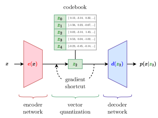
In this paper, we propose a novel tokenizer that utilizes a vector-quantized variational auto-encoder (VQ-VAE; van den Oord et al., 2017) as its central component. VQ-VAE is a powerful technique for learning discrete latent variables that can encode words and reconstruct them back to their original form. This process can be broken down into three main steps, as illustrated in Figure 1:

1.

The encoder maps the data samples (subwords) $\bm{x}$ to continuous latent vectors $\color[rgb]{1.0,0.0,0.3}\definecolor[named]{pgfstrokecolor}{rgb}{1.0,0.0,0.3}e(\color[rgb]{0,0,0}\definecolor[named]{pgfstrokecolor}{rgb}{0,0,0}\pgfsys@color@gray@stroke{0}\pgfsys@color@gray@fill{0}\bm{x}\color[rgb]{1.0,0.0,0.3}\definecolor[named]{pgfstrokecolor}{rgb}{1.0,0.0,0.3})$ .
2.

The codebook is made up of $K$ codebook vectors $\color[rgb]{0,0.6,0}\definecolor[named]{pgfstrokecolor}{rgb}{0,0.6,0}\bm{z}_{\color[rgb]{0,0,0}\definecolor[named]{pgfstrokecolor}{rgb}{0,0,0}\pgfsys@color@gray@stroke{0}\pgfsys@color@gray@fill{0}k}\color[rgb]{0,0,0}\definecolor[named]{pgfstrokecolor}{rgb}{0,0,0}\pgfsys@color@gray@stroke{0}\pgfsys@color@gray@fill{0},k\in 1\dots K$ . Each latent vector $\color[rgb]{1.0,0.0,0.3}\definecolor[named]{pgfstrokecolor}{rgb}{1.0,0.0,0.3}e(\color[rgb]{0,0,0}\definecolor[named]{pgfstrokecolor}{rgb}{0,0,0}\pgfsys@color@gray@stroke{0}\pgfsys@color@gray@fill{0}\bm{x}\color[rgb]{1.0,0.0,0.3}\definecolor[named]{pgfstrokecolor}{rgb}{1.0,0.0,0.3})$ is quantized to its nearest codebook vector $\color[rgb]{0,0.6,0}\definecolor[named]{pgfstrokecolor}{rgb}{0,0.6,0}\bm{z}_{\color[rgb]{0,0,0}\definecolor[named]{pgfstrokecolor}{rgb}{0,0,0}\pgfsys@color@gray@stroke{0}\pgfsys@color@gray@fill{0}k}$ , effectively mapping each input sample $\bm{x}$ onto a discrete variable $k$ . The encoder and codebook downsample and compress the information in $\bm{x}$ , serving as an information bottleneck Tishby et al. (1999).
3.

The decoder reconstructs the symbols $\color[rgb]{0,0.6,0}\definecolor[named]{pgfstrokecolor}{rgb}{0,0.6,0}\bm{z}$ back into the original input distribution, modeling the distribution $p(\bm{x}|\color[rgb]{0,0.6,0}\definecolor[named]{pgfstrokecolor}{rgb}{0,0.6,0}\bm{z}\color[rgb]{0,0,0}\definecolor[named]{pgfstrokecolor}{rgb}{0,0,0}\pgfsys@color@gray@stroke{0}\pgfsys@color@gray@fill{0})$ as $\color[rgb]{0,0.3,1.0}\definecolor[named]{pgfstrokecolor}{rgb}{0,0.3,1.0}d(\color[rgb]{0,0.6,0}\definecolor[named]{pgfstrokecolor}{rgb}{0,0.6,0}\bm{z}\color[rgb]{0,0.3,1.0}\definecolor[named]{pgfstrokecolor}{rgb}{0,0.3,1.0})$ .

Gradient backpropagation.

The model is optimized jointly with the backpropagation algorithm. However, special attention must be given to the codebook quantization $\color[rgb]{0,0.6,0}\definecolor[named]{pgfstrokecolor}{rgb}{0,0.6,0}q$ as this operation is not differentiable:

\begin{split}\color[rgb]{0,0.6,0}\definecolor[named]{pgfstrokecolor}{rgb}{0,0.6,0}q\!\left(\color[rgb]{1.0,0.0,0.3}\definecolor[named]{pgfstrokecolor}{rgb}{1.0,0.0,0.3}e(\color[rgb]{0,0,0}\definecolor[named]{pgfstrokecolor}{rgb}{0,0,0}\pgfsys@color@gray@stroke{0}\pgfsys@color@gray@fill{0}\bm{x}\color[rgb]{1.0,0.0,0.3}\definecolor[named]{pgfstrokecolor}{rgb}{1.0,0.0,0.3})\color[rgb]{0,0.6,0}\definecolor[named]{pgfstrokecolor}{rgb}{0,0.6,0}\right)\color[rgb]{0,0,0}\definecolor[named]{pgfstrokecolor}{rgb}{0,0,0}\pgfsys@color@gray@stroke{0}\pgfsys@color@gray@fill{0}&=\color[rgb]{0,0.6,0}\definecolor[named]{pgfstrokecolor}{rgb}{0,0.6,0}\bm{z}_{\color[rgb]{0,0,0}\definecolor[named]{pgfstrokecolor}{rgb}{0,0,0}\pgfsys@color@gray@stroke{0}\pgfsys@color@gray@fill{0}k}\color[rgb]{0,0,0}\definecolor[named]{pgfstrokecolor}{rgb}{0,0,0}\pgfsys@color@gray@stroke{0}\pgfsys@color@gray@fill{0},\,\,\textrm{where}\\ k&=\operatorname*{argmin}_{i}{\lVert\color[rgb]{1.0,0.0,0.3}\definecolor[named]{pgfstrokecolor}{rgb}{1.0,0.0,0.3}e(\color[rgb]{0,0,0}\definecolor[named]{pgfstrokecolor}{rgb}{0,0,0}\pgfsys@color@gray@stroke{0}\pgfsys@color@gray@fill{0}\bm{x}\color[rgb]{1.0,0.0,0.3}\definecolor[named]{pgfstrokecolor}{rgb}{1.0,0.0,0.3})\color[rgb]{0,0,0}\definecolor[named]{pgfstrokecolor}{rgb}{0,0,0}\pgfsys@color@gray@stroke{0}\pgfsys@color@gray@fill{0}-\color[rgb]{0,0.6,0}\definecolor[named]{pgfstrokecolor}{rgb}{0,0.6,0}\bm{z}\color[rgb]{0,0,0}\definecolor[named]{pgfstrokecolor}{rgb}{0,0,0}\pgfsys@color@gray@stroke{0}\pgfsys@color@gray@fill{0}_{i}\rVert_{2}}\\ \end{split}

(1)

During the forward phase, the quantized codebook vectors are simply passed to the decoder. However, during the backward phase, the gradient of the loss function $\nabla_{\!\color[rgb]{0,0.3,1.0}\definecolor[named]{pgfstrokecolor}{rgb}{0,0.3,1.0}d\color[rgb]{0,0,0}\definecolor[named]{pgfstrokecolor}{rgb}{0,0,0}\pgfsys@color@gray@stroke{0}\pgfsys@color@gray@fill{0}}\mathcal{L}$ is passed directly from the decoder to the encoder. This technique, known as straight-through gradient estimation, is possible because the output of the encoder and the input of the decoder share the same latent space. The output $\color[rgb]{1.0,0.0,0.3}\definecolor[named]{pgfstrokecolor}{rgb}{1.0,0.0,0.3}e(\color[rgb]{0,0,0}\definecolor[named]{pgfstrokecolor}{rgb}{0,0,0}\pgfsys@color@gray@stroke{0}\pgfsys@color@gray@fill{0}\bm{x}\color[rgb]{1.0,0.0,0.3}\definecolor[named]{pgfstrokecolor}{rgb}{1.0,0.0,0.3})$ is sufficiently similar to the decoder input $\bm{z}$ , such that the gradient carries information about how to change $\color[rgb]{1.0,0.0,0.3}\definecolor[named]{pgfstrokecolor}{rgb}{1.0,0.0,0.3}e(\color[rgb]{0,0,0}\definecolor[named]{pgfstrokecolor}{rgb}{0,0,0}\pgfsys@color@gray@stroke{0}\pgfsys@color@gray@fill{0}\bm{x}\color[rgb]{1.0,0.0,0.3}\definecolor[named]{pgfstrokecolor}{rgb}{1.0,0.0,0.3})$ to lower the reconstruction loss.

Loss terms.

In addition to the standard reconstruction loss $\mathcal{L}_{r}=\textrm{log}\,p(\bm{x}|\color[rgb]{0,0.6,0}\definecolor[named]{pgfstrokecolor}{rgb}{0,0.6,0}\bm{z}\color[rgb]{0,0,0}\definecolor[named]{pgfstrokecolor}{rgb}{0,0,0}\pgfsys@color@gray@stroke{0}\pgfsys@color@gray@fill{0})$ , which measures the auto-encoding performance, the VQ-VAE model incorporates two auxiliary loss terms that align the encoder outputs $\color[rgb]{1.0,0.0,0.3}\definecolor[named]{pgfstrokecolor}{rgb}{1.0,0.0,0.3}e(\color[rgb]{0,0,0}\definecolor[named]{pgfstrokecolor}{rgb}{0,0,0}\pgfsys@color@gray@stroke{0}\pgfsys@color@gray@fill{0}\bm{x}\color[rgb]{1.0,0.0,0.3}\definecolor[named]{pgfstrokecolor}{rgb}{1.0,0.0,0.3})$ with the nearest codebook vectors. Specifically, the codebook loss is defined as $\mathcal{L}_{\color[rgb]{0,0.6,0}\definecolor[named]{pgfstrokecolor}{rgb}{0,0.6,0}q}=\lVert\textrm{sg}(\color[rgb]{1.0,0.0,0.3}\definecolor[named]{pgfstrokecolor}{rgb}{1.0,0.0,0.3}e(\color[rgb]{0,0,0}\definecolor[named]{pgfstrokecolor}{rgb}{0,0,0}\pgfsys@color@gray@stroke{0}\pgfsys@color@gray@fill{0}\bm{x}\color[rgb]{1.0,0.0,0.3}\definecolor[named]{pgfstrokecolor}{rgb}{1.0,0.0,0.3})\color[rgb]{0,0,0}\definecolor[named]{pgfstrokecolor}{rgb}{0,0,0}\pgfsys@color@gray@stroke{0}\pgfsys@color@gray@fill{0})-\color[rgb]{0,0.6,0}\definecolor[named]{pgfstrokecolor}{rgb}{0,0.6,0}\bm{z}\color[rgb]{0,0,0}\definecolor[named]{pgfstrokecolor}{rgb}{0,0,0}\pgfsys@color@gray@stroke{0}\pgfsys@color@gray@fill{0}_{k}\rVert_{2}$ and the commitment loss as $\mathcal{L}_{\color[rgb]{1.0,0.0,0.3}\definecolor[named]{pgfstrokecolor}{rgb}{1.0,0.0,0.3}e}=\lVert\color[rgb]{1.0,0.0,0.3}\definecolor[named]{pgfstrokecolor}{rgb}{1.0,0.0,0.3}e(\color[rgb]{0,0,0}\definecolor[named]{pgfstrokecolor}{rgb}{0,0,0}\pgfsys@color@gray@stroke{0}\pgfsys@color@gray@fill{0}\bm{x}\color[rgb]{1.0,0.0,0.3}\definecolor[named]{pgfstrokecolor}{rgb}{1.0,0.0,0.3})\color[rgb]{0,0,0}\definecolor[named]{pgfstrokecolor}{rgb}{0,0,0}\pgfsys@color@gray@stroke{0}\pgfsys@color@gray@fill{0}-\textrm{sg}(\color[rgb]{0,0.6,0}\definecolor[named]{pgfstrokecolor}{rgb}{0,0.6,0}\bm{z}\color[rgb]{0,0,0}\definecolor[named]{pgfstrokecolor}{rgb}{0,0,0}\pgfsys@color@gray@stroke{0}\pgfsys@color@gray@fill{0}_{k})\rVert_{2}$ , where ‘sg’ is the stop gradient operation and $\color[rgb]{0,0.6,0}\definecolor[named]{pgfstrokecolor}{rgb}{0,0.6,0}\bm{z}\color[rgb]{0,0,0}\definecolor[named]{pgfstrokecolor}{rgb}{0,0,0}\pgfsys@color@gray@stroke{0}\pgfsys@color@gray@fill{0}_{k}$ is the codebook vector defined in Equation 1. The overall loss of a VQ-VAE model is computed as:

\mathcal{L}=\mathcal{L}_{r}+\mathcal{L}_{\color[rgb]{0,0.6,0}\definecolor[named]{pgfstrokecolor}{rgb}{0,0.6,0}q}+\beta\mathcal{L}_{\color[rgb]{1.0,0.0,0.3}\definecolor[named]{pgfstrokecolor}{rgb}{1.0,0.0,0.3}e},

where $\beta$ is a hyperparameter that balances the focus between reconstruction and codebook alignment.

Refer to caption — Figure 1: The main components of a VQ-VAE model. The latent vector $\color[rgb]{1.0,0.0,0.3}\definecolor[named]{pgfstrokecolor}{rgb}{1.0,0.0,0.3}e(\color[rgb]{0,0,0}\definecolor[named]{pgfstrokecolor}{rgb}{0,0,0}\pgfsys@color@gray@stroke{0}\pgfsys@color@gray@fill{0}\bm{x}\color[rgb]{1.0,0.0,0.3}\definecolor[named]{pgfstrokecolor}{rgb}{1.0,0.0,0.3})$ is quantized into the 2^nd codebook vector $\color[rgb]{0,0.6,0}\definecolor[named]{pgfstrokecolor}{rgb}{0,0.6,0}\bm{z}\color[rgb]{0,0,0}\definecolor[named]{pgfstrokecolor}{rgb}{0,0,0}\pgfsys@color@gray@stroke{0}\pgfsys@color@gray@fill{0}_{2}$ and then the decoder tries to reconstruct the original input as $\color[rgb]{0,0.3,1.0}\definecolor[named]{pgfstrokecolor}{rgb}{0,0.3,1.0}d(\color[rgb]{0,0.6,0}\definecolor[named]{pgfstrokecolor}{rgb}{0,0.6,0}\bm{z}\color[rgb]{0,0,0}\definecolor[named]{pgfstrokecolor}{rgb}{0,0,0}\pgfsys@color@gray@stroke{0}\pgfsys@color@gray@fill{0}_{2}\color[rgb]{0,0.3,1.0}\definecolor[named]{pgfstrokecolor}{rgb}{0,0.3,1.0})$ . We use the codebook size $K=5$ in this illustrative example, i.e. all vectors are clustered into five possible values.

Codebook EMA.

An alternative approach to updating the codebook, proposed by van den Oord et al. (2017), is to update it as an exponential moving average (EMA) of the latent variables $\color[rgb]{1.0,0.0,0.3}\definecolor[named]{pgfstrokecolor}{rgb}{1.0,0.0,0.3}e(\color[rgb]{0,0,0}\definecolor[named]{pgfstrokecolor}{rgb}{0,0,0}\pgfsys@color@gray@stroke{0}\pgfsys@color@gray@fill{0}\bm{x}\color[rgb]{1.0,0.0,0.3}\definecolor[named]{pgfstrokecolor}{rgb}{1.0,0.0,0.3})\color[rgb]{0,0,0}\definecolor[named]{pgfstrokecolor}{rgb}{0,0,0}\pgfsys@color@gray@stroke{0}\pgfsys@color@gray@fill{0}$ – instead of incorporating the codebook loss $\mathcal{L}_{\color[rgb]{0,0.6,0}\definecolor[named]{pgfstrokecolor}{rgb}{0,0.6,0}q}$ . This update consists of updating two variables: the codebook usage counts $c_{k}$ and the codebook vectors $\color[rgb]{0,0.6,0}\definecolor[named]{pgfstrokecolor}{rgb}{0,0.6,0}\bm{z}_{\color[rgb]{0,0,0}\definecolor[named]{pgfstrokecolor}{rgb}{0,0,0}\pgfsys@color@gray@stroke{0}\pgfsys@color@gray@fill{0}k}$ , where $\lambda$ is the EMA decay hyperparameter:

\begin{split}c_{k}&\leftarrow\lambda c_{k}+(1-\lambda)\sum_{i}{\mathbbm{1}_{\left[\color[rgb]{0,0.6,0}\definecolor[named]{pgfstrokecolor}{rgb}{0,0.6,0}q(\color[rgb]{1.0,0.0,0.3}\definecolor[named]{pgfstrokecolor}{rgb}{1.0,0.0,0.3}e(\color[rgb]{0,0,0}\definecolor[named]{pgfstrokecolor}{rgb}{0,0,0}\pgfsys@color@gray@stroke{0}\pgfsys@color@gray@fill{0}\bm{x}_{i}\color[rgb]{1.0,0.0,0.3}\definecolor[named]{pgfstrokecolor}{rgb}{1.0,0.0,0.3})\color[rgb]{0,0.6,0}\definecolor[named]{pgfstrokecolor}{rgb}{0,0.6,0})\color[rgb]{0,0,0}\definecolor[named]{pgfstrokecolor}{rgb}{0,0,0}\pgfsys@color@gray@stroke{0}\pgfsys@color@gray@fill{0}\,=\,\color[rgb]{0,0.6,0}\definecolor[named]{pgfstrokecolor}{rgb}{0,0.6,0}\bm{z}\color[rgb]{0,0,0}\definecolor[named]{pgfstrokecolor}{rgb}{0,0,0}\pgfsys@color@gray@stroke{0}\pgfsys@color@gray@fill{0}_{k}\right]}}\\ \color[rgb]{0,0.6,0}\definecolor[named]{pgfstrokecolor}{rgb}{0,0.6,0}\bm{z}\color[rgb]{0,0,0}\definecolor[named]{pgfstrokecolor}{rgb}{0,0,0}\pgfsys@color@gray@stroke{0}\pgfsys@color@gray@fill{0}_{k}&\leftarrow\lambda\color[rgb]{0,0.6,0}\definecolor[named]{pgfstrokecolor}{rgb}{0,0.6,0}\bm{z}\color[rgb]{0,0,0}\definecolor[named]{pgfstrokecolor}{rgb}{0,0,0}\pgfsys@color@gray@stroke{0}\pgfsys@color@gray@fill{0}_{k}+\frac{(1-\lambda)}{c_{k}}\sum_{i}{\color[rgb]{1.0,0.0,0.3}\definecolor[named]{pgfstrokecolor}{rgb}{1.0,0.0,0.3}e(\color[rgb]{0,0,0}\definecolor[named]{pgfstrokecolor}{rgb}{0,0,0}\pgfsys@color@gray@stroke{0}\pgfsys@color@gray@fill{0}\bm{x}_{i}\color[rgb]{1.0,0.0,0.3}\definecolor[named]{pgfstrokecolor}{rgb}{1.0,0.0,0.3})\color[rgb]{0,0,0}\definecolor[named]{pgfstrokecolor}{rgb}{0,0,0}\pgfsys@color@gray@stroke{0}\pgfsys@color@gray@fill{0}\mathbbm{1}_{\left[\color[rgb]{0,0.6,0}\definecolor[named]{pgfstrokecolor}{rgb}{0,0.6,0}q(\color[rgb]{1.0,0.0,0.3}\definecolor[named]{pgfstrokecolor}{rgb}{1.0,0.0,0.3}e(\color[rgb]{0,0,0}\definecolor[named]{pgfstrokecolor}{rgb}{0,0,0}\pgfsys@color@gray@stroke{0}\pgfsys@color@gray@fill{0}\bm{x}_{i}\color[rgb]{1.0,0.0,0.3}\definecolor[named]{pgfstrokecolor}{rgb}{1.0,0.0,0.3})\color[rgb]{0,0.6,0}\definecolor[named]{pgfstrokecolor}{rgb}{0,0.6,0})\color[rgb]{0,0,0}\definecolor[named]{pgfstrokecolor}{rgb}{0,0,0}\pgfsys@color@gray@stroke{0}\pgfsys@color@gray@fill{0}\,=\,\color[rgb]{0,0.6,0}\definecolor[named]{pgfstrokecolor}{rgb}{0,0.6,0}\bm{z}\color[rgb]{0,0,0}\definecolor[named]{pgfstrokecolor}{rgb}{0,0,0}\pgfsys@color@gray@stroke{0}\pgfsys@color@gray@fill{0}_{k}\right]}}\end{split}

This approach leads to more stable training (Kaiser et al., 2018) and it allows us to mitigate the codebook collapse, which occurs when the usage count of a vector drops to zero and the vector is then never updated (Kaiser et al., 2018). Thus, whenever a codebook vector $\color[rgb]{0,0.6,0}\definecolor[named]{pgfstrokecolor}{rgb}{0,0.6,0}\bm{z}\color[rgb]{0,0,0}\definecolor[named]{pgfstrokecolor}{rgb}{0,0,0}\pgfsys@color@gray@stroke{0}\pgfsys@color@gray@fill{0}_{i}$ has usage $\bm{c}_{i}$ lower than $c_{\textrm{min}}$ , it is reassigned to a random latent vector $\color[rgb]{0,0.6,0}\definecolor[named]{pgfstrokecolor}{rgb}{0,0.6,0}\bm{z}\color[rgb]{0,0,0}\definecolor[named]{pgfstrokecolor}{rgb}{0,0,0}\pgfsys@color@gray@stroke{0}\pgfsys@color@gray@fill{0}_{i}\leftarrow\color[rgb]{1.0,0.0,0.3}\definecolor[named]{pgfstrokecolor}{rgb}{1.0,0.0,0.3}e(\color[rgb]{0,0,0}\definecolor[named]{pgfstrokecolor}{rgb}{0,0,0}\pgfsys@color@gray@stroke{0}\pgfsys@color@gray@fill{0}\bm{x}_{j}\color[rgb]{1.0,0.0,0.3}\definecolor[named]{pgfstrokecolor}{rgb}{1.0,0.0,0.3})$ and the usage count is reset $c_{i}\leftarrow 1$ , similar to Williams et al. (2020) or Dhariwal et al. (2020).

3 Factorizer

We utilize the VQ-VAE architecture to train a model capable of mapping discrete triplet representations $\color[rgb]{0,0.6,0}\definecolor[named]{pgfstrokecolor}{rgb}{0,0.6,0}\bm{z}$ to subword strings $\bm{w}$ (and vice versa). Furthermore, we employ the VQ-VAE decoder to estimate the probabilities of the subword strings $p(\bm{w}|\color[rgb]{0,0.6,0}\definecolor[named]{pgfstrokecolor}{rgb}{0,0.6,0}\bm{z}\color[rgb]{0,0,0}\definecolor[named]{pgfstrokecolor}{rgb}{0,0,0}\pgfsys@color@gray@stroke{0}\pgfsys@color@gray@fill{0})$ . After the model is trained, we infer its vocabulary, consisting of a set of tuples $\langle\bm{w}_{i},\color[rgb]{0,0.6,0}\definecolor[named]{pgfstrokecolor}{rgb}{0,0.6,0}\bm{z}\color[rgb]{0,0,0}\definecolor[named]{pgfstrokecolor}{rgb}{0,0,0}\pgfsys@color@gray@stroke{0}\pgfsys@color@gray@fill{0}_{i},\textrm{log}\,p(\bm{w}_{i}|\color[rgb]{0,0.6,0}\definecolor[named]{pgfstrokecolor}{rgb}{0,0.6,0}\bm{z}\color[rgb]{0,0,0}\definecolor[named]{pgfstrokecolor}{rgb}{0,0,0}\pgfsys@color@gray@stroke{0}\pgfsys@color@gray@fill{0}_{i})\rangle$ . Finally, we use this vocabulary to perform optimal (in regards to the log-probabilities) subword tokenization.

3.1 VQ-VAE subword encoding

Training data.

The auto-encoder is trained on a word-frequency list obtained by word-tokenizing a large text corpus. Let us denote the frequency of word $\bm{w}$ by $f_{\bm{w}}$ . Note that while this data representation simplifies the model by discarding any contextual information, it still enables proper estimation of $p(\bm{w}_{i}|\color[rgb]{0,0.6,0}\definecolor[named]{pgfstrokecolor}{rgb}{0,0.6,0}\bm{z}\color[rgb]{0,0,0}\definecolor[named]{pgfstrokecolor}{rgb}{0,0,0}\pgfsys@color@gray@stroke{0}\pgfsys@color@gray@fill{0}_{i})$ by following the word frequencies $f_{\bm{w}}$ .

Word representation.

In this study, words are represented as sequences of UTF-8 bytes. To ensure proper handling of word boundaries, the word sequences start with a special “beginning-of-word” token and end with an “end-of-word” token; both tokens are depicted as the symbol ‘␣’ in this text.

Data sampling.

In theory, the correct way of sampling the training data is to directly follow the frequencies $f_{\bm{w}}$ . However, in practice, the distribution of words in a natural language follows Zipf’s law, resulting in a skewed distribution that collapses the training process. To address this issue, we sample the data according to a more balanced distribution

p_{\textrm{sample}}(w)\propto\frac{f_{\bm{w}}}{\textrm{log}(f_{\bm{w}}+1)}.

To compensate for this alteration and accurately model the true word distribution, we incorporate the denominator into the loss function by weighting it as follows:

\mathcal{L}=\sum_{\bm{w}}{\textrm{log}(f_{\bm{w}}+1)\,\mathcal{L}(\bm{w})}.

Subword splitting.

Up to this point, we have only discussed word encoding. To also encode subwords, we randomly split some of the sampled words into subwords. Specifically, as the more frequent words should be split less frequently, we keep the word as-is with the probability

p_{\textrm{not-split}}(w)=\frac{\textrm{log}(f_{\bm{w}}+1)}{\textrm{max}_{\bm{x}}\,\textrm{log}(f_{\bm{x}}+1)}.

Factorized codebooks.

To capture fine-grained information about the characters inside words, we employ separate codebooks, each within a unique latent space. In addition, to further reduce the issue of codebook collapse, each codebook consists only of $K=256$ codebook vectors.³³3Note that this is reminiscent of the standard 24-bit RGB color encoding, where every codebook triplet can be viewed as an RGB color. Factorizer essentially projects subwords into a color space, see Appendix A for more details.

Backbone architecture.

The auto-encoder model is based on an encoder-decoder transformer architecture (Vaswani et al., 2017) with three quantization bottlenecks. Specifically, we first pad the byte-tokens $\bm{w}$ with special R, G, B prior tokens, then embed and encode each sequence with a transformer encoder. The contextualized embedding vectors for the first three tokens serve as the encoding $\color[rgb]{1.0,0.0,0.3}\definecolor[named]{pgfstrokecolor}{rgb}{1.0,0.0,0.3}e(\color[rgb]{0,0,0}\definecolor[named]{pgfstrokecolor}{rgb}{0,0,0}\pgfsys@color@gray@stroke{0}\pgfsys@color@gray@fill{0}\bm{w}\color[rgb]{1.0,0.0,0.3}\definecolor[named]{pgfstrokecolor}{rgb}{1.0,0.0,0.3})$ . These three vectors are then quantized and prepended to the subword byte-tokens $\bm{w}$ , which are finally input into the autoregressive transformer decoder $\color[rgb]{0,0.3,1.0}\definecolor[named]{pgfstrokecolor}{rgb}{0,0.3,1.0}d(\color[rgb]{0,0.6,0}\definecolor[named]{pgfstrokecolor}{rgb}{0,0.6,0}\bm{z}\color[rgb]{0,0,0}\definecolor[named]{pgfstrokecolor}{rgb}{0,0,0}\pgfsys@color@gray@stroke{0}\pgfsys@color@gray@fill{0},\bm{w}\color[rgb]{0,0.3,1.0}\definecolor[named]{pgfstrokecolor}{rgb}{0,0.3,1.0})$ , modeling $p(\bm{w}|\color[rgb]{0,0.6,0}\definecolor[named]{pgfstrokecolor}{rgb}{0,0.6,0}\bm{z}\color[rgb]{0,0,0}\definecolor[named]{pgfstrokecolor}{rgb}{0,0,0}\pgfsys@color@gray@stroke{0}\pgfsys@color@gray@fill{0})$ .

Training details.

All VQ-VAE models in this study utilize a transformer with 6 layers and 256 hidden size for both the encoder and decoder. The models are trained for 50 000 steps with batch size of 4 096 and optimized with adaptive sharpness-aware minimization (ASAM; Kwon et al., 2021) to ensure better generalization to unseen words, with AdamW (Loshchilov and Hutter, 2019) as the underlying optimizer. To further improve generalization, we calculate the exponential moving average of the parameters (with a decay of 0.999) and use this average for inference. For more details about the transformer architecture and hyperparameters, please refer to Samuel et al. (2023) and Appendix D.

Vocabulary construction.

The VQ-VAE is not used directly for tokenization as that would greatly slow it down. Instead, we infer its static vocabulary by iterating through all $256^{3}$ instances of the RGB codebooks. The subword vocabulary is decoded as

\mathcal{W}=\left\{\operatorname*{argmax}_{\bm{w}}p(\bm{w}|\color[rgb]{0,0.6,0}\definecolor[named]{pgfstrokecolor}{rgb}{0,0.6,0}\bm{z}\color[rgb]{0,0,0}\definecolor[named]{pgfstrokecolor}{rgb}{0,0,0}\pgfsys@color@gray@stroke{0}\pgfsys@color@gray@fill{0})\,\,\middle|\,\,\color[rgb]{0,0.6,0}\definecolor[named]{pgfstrokecolor}{rgb}{0,0.6,0}\bm{z}\color[rgb]{0,0,0}\definecolor[named]{pgfstrokecolor}{rgb}{0,0,0}\pgfsys@color@gray@stroke{0}\pgfsys@color@gray@fill{0}\in[256]^{3}\!,\,\,p(\color[rgb]{0,0.6,0}\definecolor[named]{pgfstrokecolor}{rgb}{0,0.6,0}\bm{z}\color[rgb]{0,0,0}\definecolor[named]{pgfstrokecolor}{rgb}{0,0,0}\pgfsys@color@gray@stroke{0}\pgfsys@color@gray@fill{0})\!>\!0\right\}\!,

where the prior distribution $p(\color[rgb]{0,0.6,0}\definecolor[named]{pgfstrokecolor}{rgb}{0,0.6,0}\bm{z}\color[rgb]{0,0,0}\definecolor[named]{pgfstrokecolor}{rgb}{0,0,0}\pgfsys@color@gray@stroke{0}\pgfsys@color@gray@fill{0})$ is calculated by counting the usage of all codebook triplets throughout training. Finally, the full vocabulary $\mathcal{V}$ is a set of tuples $\langle\bm{w}_{i},\color[rgb]{0,0.6,0}\definecolor[named]{pgfstrokecolor}{rgb}{0,0.6,0}\bm{z}\color[rgb]{0,0,0}\definecolor[named]{pgfstrokecolor}{rgb}{0,0,0}\pgfsys@color@gray@stroke{0}\pgfsys@color@gray@fill{0}_{i},\textrm{log}\,p(\bm{w}_{i}|\color[rgb]{0,0.6,0}\definecolor[named]{pgfstrokecolor}{rgb}{0,0.6,0}\bm{z}\color[rgb]{0,0,0}\definecolor[named]{pgfstrokecolor}{rgb}{0,0,0}\pgfsys@color@gray@stroke{0}\pgfsys@color@gray@fill{0}_{i})\rangle$ , where $\bm{w}_{i}\in\mathcal{W}$ and $\color[rgb]{0,0.6,0}\definecolor[named]{pgfstrokecolor}{rgb}{0,0.6,0}\bm{z}\color[rgb]{0,0,0}\definecolor[named]{pgfstrokecolor}{rgb}{0,0,0}\pgfsys@color@gray@stroke{0}\pgfsys@color@gray@fill{0}_{i}=\operatorname*{argmax}_{\color[rgb]{0,0.6,0}\definecolor[named]{pgfstrokecolor}{rgb}{0,0.6,0}\bm{z}}p(\bm{w}_{i}|\color[rgb]{0,0.6,0}\definecolor[named]{pgfstrokecolor}{rgb}{0,0.6,0}\bm{z}\color[rgb]{0,0,0}\definecolor[named]{pgfstrokecolor}{rgb}{0,0,0}\pgfsys@color@gray@stroke{0}\pgfsys@color@gray@fill{0})$ .

3.2 Subword tokenizer

Optimal split search.

After inferring the vocabulary $\mathcal{V}$ , we can search for the optimal tokenization of a word $\bm{x}$ into subwords $\bm{w}_{1},\bm{w}_{2},\dots\bm{w}_{k}$ :

\textrm{tokenize}(\bm{x})=\operatorname*{argmin}_{\bm{w}_{1}\!\bm{w}_{2}\dots\bm{w}_{k}\,=\,\bm{x}}\,\,{\sum_{i=1}^{k}{\textrm{score}(\bm{w}_{i})}},\hskip 5.0pt

where for each subword $\bm{w}_{i}$ from the vocabulary triplets $\langle\bm{w}_{i},\color[rgb]{0,0.6,0}\definecolor[named]{pgfstrokecolor}{rgb}{0,0.6,0}\bm{z}\color[rgb]{0,0,0}\definecolor[named]{pgfstrokecolor}{rgb}{0,0,0}\pgfsys@color@gray@stroke{0}\pgfsys@color@gray@fill{0}_{i},\textrm{log}\,p(\bm{w}_{i}|\color[rgb]{0,0.6,0}\definecolor[named]{pgfstrokecolor}{rgb}{0,0.6,0}\bm{z}\color[rgb]{0,0,0}\definecolor[named]{pgfstrokecolor}{rgb}{0,0,0}\pgfsys@color@gray@stroke{0}\pgfsys@color@gray@fill{0}_{i})\rangle\in\mathcal{V}$ , its score is

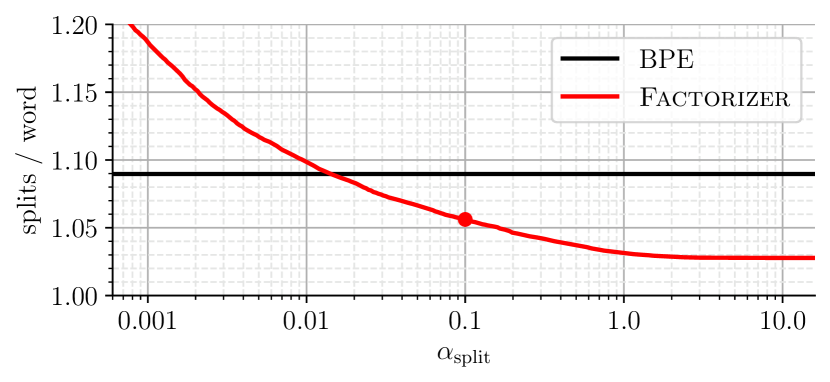
\textrm{score}(\bm{w}_{i})=-\textrm{log}\,p(\bm{w}_{i}|\color[rgb]{0,0.6,0}\definecolor[named]{pgfstrokecolor}{rgb}{0,0.6,0}\bm{z}_{i}\color[rgb]{0,0,0}\definecolor[named]{pgfstrokecolor}{rgb}{0,0,0}\pgfsys@color@gray@stroke{0}\pgfsys@color@gray@fill{0})+\alpha_{\textrm{split}}.\hskip 13.99995pt

The parameter $\alpha_{\textrm{split}}$ allows for a smooth change of the amount of splits per word, as shown in Figure 3. We use $\alpha_{\textrm{split}}=0.1$ for all experiments in this work.

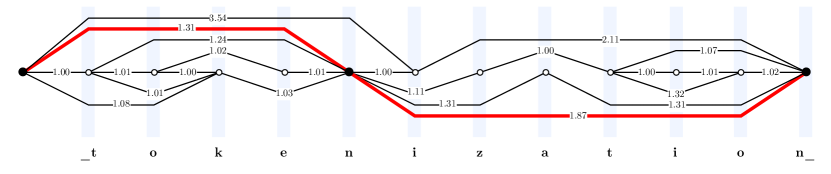
The tokenize function is implemented via the shortest path search in a tokenization graph, as illustrated in Figure 2. Specifically, the search uses Dijkstra’s algorithm (Dijkstra, 1959) and the forward edges from each node are efficiently iterated with the prefix search in a directed acyclic word graph (DAWG; Blumer et al., 1985) of all subwords from $\mathcal{V}$ . A simplified pseudocode of the search algorithm is given below, the optimal tokenization is then obtained by reverse iteration of the returned prev dictionary.

⬇

def search(|\bfseries{\color{Grey}word}|, |\bfseries{\color{Grey}dawg\_trie}|):

|\bfseries{\color{Grey}Q}|.append(|\bfseries{\color{Grey}word}|) |\textit{\color{Grey}priority queue of suffixes}|

|\bfseries{\color{Grey}cost}|[|\bfseries{\color{Grey}word}|] = 0.0 |\textit{\color{Grey}cost returns +inf by default}|

|\bfseries{\color{Grey}prev}|[|\bfseries{\color{Grey}word}|] = none | \textit{\color{Grey}pointers to predecesors}|

\parwhile |\bfseries{\color{Grey}Q}| |\texttt{is not empty}|:

|\bfseries{\color{Grey}suffix}| = suffix |\texttt{from}| |\bfseries{\color{Grey}Q}| |\texttt{with}| minimal |\bfseries{\color{Grey}cost}|

remove |\bfseries{\color{Grey}suffix}| |\texttt{from}| |\bfseries{\color{Grey}Q}|

if |\bfseries{\color{Grey}suffix}| |\texttt{is}| empty: break

\parfor every |\bfseries{\color{Grey}prefix}| of |\bfseries{\color{Grey}suffix}| |\texttt{in}| |\bfseries{\color{Grey}dawg\_trie}|:

|\bfseries{\color{Grey}new\_cost}| = |\bfseries{\color{Grey}cost}|[|\bfseries{\color{Grey}suffix}|] + score(|\bfseries{\color{Grey}prefix}|)

|\bfseries{\color{Grey}new\_suffix}| = |\bfseries{\color{Grey}suffix}|[len(|\bfseries{\color{Grey}prefix}|):]

if |\bfseries{\color{Grey}new\_cost}| < |\bfseries{\color{Grey}cost}|[|\bfseries{\color{Grey}new\_suffix}|]:

|\bfseries{\color{Grey}Q}|.append(|\bfseries{\color{Grey}new\_suffix}|)

|\bfseries{\color{Grey}cost}|[|\bfseries{\color{Grey}new\_suffix}|] = |\bfseries{\color{Grey}new\_cost}|

|\bfseries{\color{Grey}prev}|[|\bfseries{\color{Grey}new\_suffix}|] = |\bfseries{\color{Grey}min\_suffix}|

\parreturn |\bfseries{\color{Grey}prev}|

Sampling.

Our formulation of the tokenizer allows for a straightforward modification for sampling different subword splits. This is similar to BPE dropout (Provilkov et al., 2020), a powerful regularization technique. The sampling works by modifying the score function as follows, making sure that all scores are non-negative so that the correctness of the search method holds:

\begin{split}\textrm{score}(\bm{w}_{i})&=-\textrm{log}\,p(\bm{w}_{i}|\color[rgb]{0,0.6,0}\definecolor[named]{pgfstrokecolor}{rgb}{0,0.6,0}\bm{z}_{i}\color[rgb]{0,0,0}\definecolor[named]{pgfstrokecolor}{rgb}{0,0,0}\pgfsys@color@gray@stroke{0}\pgfsys@color@gray@fill{0})+\alpha_{\textrm{split}}+|\bm{w}_{i}|\textrm{exp}(\epsilon)\\ \epsilon&\sim\mathcal{N}(0,\sigma_{\textrm{sample}}^{2})\end{split}

We set the parameter $\sigma_{\textrm{sample}}$ to 0.02 in all sampling experiments.

3.3 Application

Embedding layer.

The three factorizer subword indices are embedded with separate embedding layers, summed and transformed with a GeLU non-linearity. In the end, we get a single embedding vector for each subword, which makes it a simple drop-in replacement for standard embedding layers.

Averaging.

The random subword sampling can be utilized for more robust inference by sampling multiple tokenizations of each data instance and averaging the predictions for each of them.

4 Experiments

The effectiveness of factorizer is experimentally verified on a typologically diverse set of languages. We train masked language models on each language and then evaluate it on morpho-syntactic tasks from the Universal Dependencies (UD) treebanks (Nivre et al., 2016). Additionally, we demonstrate that the factorizer-based language models exhibit greater robustness to noise and superior performance in low-resource settings. We present four sets of experiments in this section:

1.

In order to provide some initial observations, we evaluate simple parsing models that do not rely on any pretrained embeddings.
2.

Then, we ablate different tokenizer configurations with English language modeling and UD finetuning.
3.

As the main experiment, we pretrain and finetune language models on 7 typologically diverse languages.
4.

Lastly, controlled experiments on English examine the robustness of our method to noise and data scarcity.

Languages.

In total, our method is evaluated on 7 different languages to investigate its performance on different morphological typologies. For the most part, we follow Vania and Lopez (2017) in their selection of languages according to the traditional categories of morphological systems. The text corpus for each language is drawn from the respective part of the mC4 corpora (Xue et al., 2021), unless specified otherwise. Note that we use the same corpus for training factorizer models (where we extract a word-frequency list for every language) as for training language models. The languages chosen for evaluation are:

•

Arabic – The first distinct language type used for evaluation are introflexive languages. We decided to use Arabic as a representative of introflexive languages because it is arguably the most wide-spread language in this class. Arabic also tests how a tokenizer can handle a non-Latin script.
•

Chinese – A purely analytical language; evaluation on Chinese tests performance on a completely different morphological typology than the other 6 languages.
•

Czech – An Indo-European language which exhibits fusional features and a rich system of morphology, typical for all Slavic languages.
•

English – In principle, also a fusional language, however, one of the most analytical languages in this class. The English corpus is made of the publicly available replications of BookCorpus and OpenWebText (because of the unnecessarily large size of the English part of mC4 for our purposes).⁴⁴4https://the-eye.eu/public/AI/pile_preliminary_components/books1.tar.gz⁵⁵5https://openwebtext2.readthedocs.io
•

Norwegian – Another Germanic language, typologically close to English, but has different morphological properties, in particular highly productive use of morphological compounding, which makes it a fitting choice for evaluation of tokenizers.
•

Scottish Gaelic – Also a fusional language. In order to evaluate performance on low-resource languages, this language, which has about 57 000 fluent speakers, was chosen as it is the smallest language from mC4 with a full train-dev-test split in Universal Dependencies.
•

Turkish – As an agglutinative language, Turkish is on the other end of the ‘morphemes-per-word spectrum’ than an analytical language like Chinese.

BPE tokenizer baseline.

We compare the performance of factorizer with the byte-pair encoding compression algorithm (BPE; Gage, 1994; Sennrich et al., 2016) as the most commonly used subword tokenizer. Following recent language modeling improvements (Radford et al., 2019), we use BPE directly on UTF-8 bytes instead of unicode characters – similarly to factorizer, which also utilizes UTF-8 bytes as the atomic unit. The training itself uses the open implementation from tokenizers library⁶⁶6https://github.com/huggingface/tokenizers and utilizes the same text corpora as the corresponding factorizer models. The choice of BPE also allows for a comparison between factorizer sampling and BPE dropout (Provilkov et al., 2020).

4.1 Experiment 1: UD parser ‘from scratch’

Before training large language models and evaluating the tokenizers in a more resource-intensive setting, we motivate our proposed method on a simple model that does not utilize any pretrained word embeddings.

UD parser architecture.

We base this first experiment on UDPipe 2, a publicly available model for PoS tagging, lemmatization and dependency parsing by Straka et al. (2019). We generally follow the original architecture, only replacing its word embeddings – UDPipe 2 utilizes a combination of pretrained contextualized embeddings, static embeddings and character embeddings – instead, we use only randomly initialized subword embeddings and learn them from scratch; the final contextualized representations for the subwords are average-pooled for each word-token to obtain word-level representations. Otherwise we use the same joint modeling approach based on bidirectional LSTM layers (Hochreiter and Schmidhuber, 1997) followed by individual classification heads for UPOS, XPOS and UFeats tagging, a classification head for relative lemma rules and a final head for dependency parsing (Dozat and Manning, 2017).

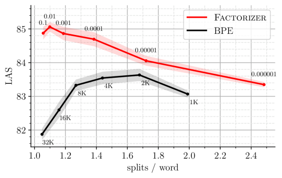
Results.

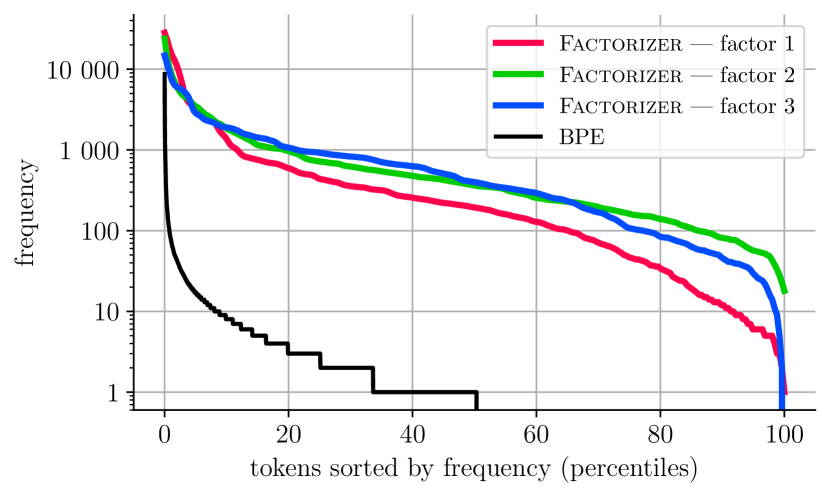
The amount of splits per word has a noticeable impact on the performance, we therefore include this dimension in the evaluation, visualized in Figure 4. This shows that factorizer is clearly a Pareto-optimal tokenizer in this comparison. We conjecture that this is caused by its ability to learn a usable embedding for less frequent, or even out-of-vocabulary subwords, as illustrated in Figure 5.

4.2 Experiment 2: Ablation study with English language modeling

In order to evaluate the performance of different BPE and factorizer configurations, we conduct a comparative study on English.

Language model pretraining.

In practice, the capabilities of a UD parser can be massively improved by utilizing contextualized embeddings from large language models that have been trained on vast amounts of data. In light of this, the main focus of this experimental section is to evaluate the impact of the factorizer on language models and their downstream performance.

We follow the training budget and parameters of the original BERT_base (Devlin et al., 2019) for pretraining the language models, the BPE-based model also uses BERT’s vocabulary size of 32K. But unlike BERT_base, we establish our models on the more efficient LTG-BERT architecture (Samuel et al., 2023), which enhances the models with some recent improvements, such as NormFormer layer normalization (Shleifer and Ott, 2022), disentangled attention with relative positional encoding (He et al., 2021) or span masking (Joshi et al., 2020). In order to reduce training time, pretraining is paralellized over 128 GPUs, the total batch size is increased to 8 192 and the amount of steps is reduced to 31 250, matching the training budget of BERT_base. Please refer Samuel et al. (2023) for details on the architecture and Appendix D for the set of all hyperparameters.

In order to make the comparison between both tokenizers fair, we approximately match the number of trainable parameters in all language models. Factorizer requires relatively small embedding layers, so we move its ‘parameter budget’ to 3 additional transformer layers – then the BPE-based models use 110.8M parameters while the factorizer-based models use 108.1M parameters in total. The effect of this choice is evaluated in Appendix B.

UD finetuning.

We employ the same model as in Section 4.1, only replacing the LSTM layers with a convex combination of hidden layers from a pretrained language model, similarly to UDify (Kondratyuk and Straka, 2019). Then we finetune the full model on a UD treebank. The detailed hyperparameter choice is given in the Appendix D.

Results.

The comparison is presented in Table 1. On average, factorizer outperforms BPE, especially in lemmatization. The results show that both sampling and averaging techniques (discussed in Section 3) improve performance, with the factorizer particularly benefiting from these features.

4.3 Experiment 3: Multi-lingual evaluation.

Finally, we train 7 BPE-based and factorizer-based language models on the selected languages and finetune them on the respective UD treebanks.

Results.

The results, displayed in Table 2, indicate that factorizer clearly achieves better performance than BPE on average. Furthermore, the factorizer is consistently more effective on lemmatization (with statistical significance), suggesting that the factorized subwords are indeed able to carry information about the characters inside the subword-units.

Interestingly, factorizer does not always perform better on Czech and Turkish, even though we hypothesized that these languages should benefit from a better character information given their rich morphology. Neither BPE or factorizer is an overall better choice for these languages.

While the results for dependency parsing in isolation (as measured by UAS and LAS) are more mixed, the parsing results which further take into account morphology (MLAS) and lemmatization (BLEX) largely favor the factorized subword encoding. Factorizer outperforms BPE (with statistical significance) in 6 out of 7 languages on BLEX scores.

Model	AllTags	Lemmas	LAS
BPE	96.05^±0.06	98.03^±0.03	92.06^±0.08
BPE + sampling	96.21^±0.04	98.25^±0.01	92.22^±0.05
BPE + sampling + averaging	96.24^±0.04	98.29^±0.04	92.22^±0.12
Factorizer	96.06^±0.05	98.01^±0.01	92.25^±0.13
Factorizer + sampling	96.29^±0.08	98.40^±0.02	92.29^±0.07
Factorizer + sampling + averaging	96.34^±0.05	98.48^±0.03	92.39^±0.14

Table 1: Comparison of BPE and factorizer configurations. The metrics are measured on the development split of en-ewt. We show the mean and standard deviation statistics over 5 random seeds, the best results are displayed in bold. Full results are shown in Table 3.

Model	UPOS	XPOS	UFeats	Lemmas	UAS	LAS	MLAS	BLEX
Arabic (ar-padt)
UDPipe 2	97.02	94.38	94.53	95.31	88.11	83.49	74.57	76.13
Stanza	62.06	54.60	68.34	49.20	42.72	39.75	39.07	38.75
BPE	97.48^±0.02	95.84^±0.03	95.97^±0.03	95.14^±0.04	90.84^±0.07	86.50^±0.07	79.03^±0.15	79.31^±0.11
Factorizer	97.48^±0.03	95.90^±0.03	96.03^±0.05	95.91^±0.04	91.24^±0.08	87.05^±0.09	79.70^±0.11	80.80^±0.11
Chinese (zh-gsd)
UDPipe 2	96.21	96.08	99.40	99.99	87.15	83.96	78.41	82.59
Stanza	95.35	95.10	99.13	99.99	81.06	77.38	72.04	76.37
BPE	97.14^±0.10	96.95^±0.10	99.60^±0.01	99.99^±0.00	88.32^±0.16	85.42^±0.20	80.23^±0.23	84.33^±0.17
Factorizer	97.00^±0.07	96.79^±0.08	99.66^±0.03	99.99^±0.00	89.34^±0.13	86.39^±0.21	81.21^±0.16	85.17^±0.17
Czech (cs-pdt)
UDPipe 2	99.45	98.47	98.40	99.28	95.63	94.23	90.88	92.50
Stanza	98.88	95.82	92.64	98.63	93.03	91.09	80.19	87.94
BPE	99.44^±0.01	98.54^±0.02	98.50^±0.02	99.26^±0.01	95.63^±0.04	94.15^±0.05	90.96^±0.05	92.42^±0.04
Factorizer	99.39^±0.01	98.53^±0.03	98.51^±0.03	99.30^±0.02	95.54^±0.04	94.10^±0.05	90.95^±0.05	92.42^±0.06
English (en-ewt)
UDPipe 2	97.35	97.06	97.52	98.07	92.62	90.56	84.02	85.98
Stanza	96.87	96.67	97.08	97.82	90.39	87.94	80.44	82.57
BPE	97.82^±0.04	97.65^±0.03	97.90^±0.04	97.99^±0.05	93.46^±0.09	91.63^±0.10	85.95^±0.14	87.21^±0.08
Factorizer	97.90^±0.07	97.72^±0.06	98.03^±0.02	98.29^±0.03	93.63^±0.12	91.80^±0.15	86.27^±0.22	87.90^±0.17
Norwegian (no-bokmaal)
UDPipe 2	98.61	—	97.68	98.82	94.40	92.91	87.59	89.43
Stanza	98.43	—	97.71	98.39	93.39	91.64	85.60	87.10
BPE	98.94^±0.02	—	98.21^±0.06	98.82^±0.02	95.42^±0.07	94.13^±0.09	89.68^±0.17	90.86^±0.10
Factorizer	98.90^±0.04	—	98.37^±0.03	99.19^±0.01	95.35^±0.09	94.05^±0.08	89.85^±0.11	91.43^±0.08
Scottish Gaelic (gd-arcosg)
UDPipe 2	96.62	92.24	94.02	97.59	87.33	81.65	69.25	75.23
Stanza	75.23	70.87	73.41	75.59	66.97	61.71	48.75	56.79
BPE	97.66^±0.06	94.96^±0.07	95.82^±0.12	97.60^±0.04	89.01^±0.08	85.63^±0.15	75.81^±0.18	79.14^±0.18
Factorizer	97.78^±0.05	95.78^±0.08	96.67^±0.09	98.09^±0.04	88.84^±0.16	85.30^±0.15	77.00^±0.22	79.85^±0.13
Turkish (tr-kenet)
UDPipe 2	93.72	—	92.06	93.33	84.07	71.29	61.92	64.89
Stanza	92.98	—	90.85	93.31	89.00	76.94	63.11	67.02
BPE	94.02^±0.10	—	92.22^±0.04	92.60^±0.10	86.35^±0.07	74.60^±0.21	65.17^±0.30	67.71^±0.25
Factorizer	93.94^±0.09	—	92.22^±0.11	92.95^±0.08	86.18^±0.04	74.49^±0.13	65.26^±0.14	68.03^±0.05
Macro average
UDPipe 2	97.00	95.89	96.23	97.48	89.90	85.44	78.10	79.53
Stanza	88.54	82.67	88.45	87.56	79.51	75.20	67.03	70.93
BPE	97.50^±0.06	96.79^±0.06	96.89^±0.06	97.34^±0.05	91.29^±0.09	87.44^±0.14	80.98^±0.19	83.00^±0.15
Factorizer	97.48^±0.06	96.94^±0.06	97.07^±0.06	97.67^±0.04	91.45^±0.10	87.60^±0.13	81.46^±0.16	83.65^±0.12

Table 2: The results of finetuning our language models on treebanks from the Universal Dependencies project – as compared to two well-performing publicly available parsers, UDPipe 2 (Straka et al., 2019) and Stanza (Qi et al., 2020). Every model is evaluated on the test split of the respective treebank, we use the official evaluation script from the CoNLL 2018 shared task (Zeman et al., 2018, https://universaldependencies.org/conll18/evaluation.html) and report the mean and standard deviation over 5 runs with different random seeds, using the gold tokenization. The best results for each language are displayed in bold. In order to compare models, we use the Almost Stochastic Order test (ASO; Del Barrio et al., 2018; Dror et al., 2019) implemented by Ulmer et al. (2022). We compare the BPE and factorizer models based on five random seeds using ASO with a confidence level of

\alpha=0.05

(before adjusting for comparison of 7 different languages using the Bonferroni correction). Almost stochastic dominance (

\epsilon_{\text{min}}<\tau

with

\tau=0.2

) is indicated by underlines.

4.4 Experiment 4: Robustness

Robustness to noise.

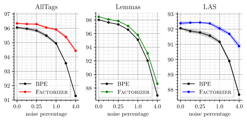
Being able to maintain performance when dealing with unnormalized and noisy text, is an important quality of any NLP tool deployed in real-world scenarios. In order to evaluate how factorizer deals with unexpected noise, we finetune a UD parser on clean data using the en-ewt corpus and evaluate it on modified development sets with increasing levels of character noise. The noise is introduced by perturbing every character with a set probability $p_{\textrm{noise}}$ by uniformly choosing from (1) deleting the character, (2) changing its letter case, or (3) repeating the character 1–3 times.

Figure 6 shows the relation between the noise level $p_{\textrm{noise}}$ and the expected performance. When comparing factorizer with BPE, it is apparent that factorizer is more robust to increased noise on tagging and dependency parsing as the performance drops more slowly with increased noise. The accuracy drops equally on lemmatization, which may be attributed to its formulation as prediction of relative lemma rules (as in UDPipe 2 by Straka et al. (2019)).

Robustness to resource scarcity.

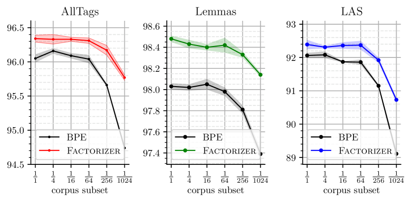
The promising results achieved on the very low-resource language of Scottish Gaelic have motivated a more thorough examination of the relationship between the size of a pretraining corpus and the downstream performance. In order to investigate this relationship, we pretrain multiple English language models using random fractions of the full English corpus while maintaining a constant number of training steps.

The performance of the finetuned models is evaluated and plotted in Figure 7. The results demonstrate that our proposed method is more robust to resource scarcity. All language models are able to maintain performance with $\nicefrac{{1}}{{64}}$ of the full corpus and after this point, the factorizer-based models are less sensitive to reducing the corpus size even more.

5 Related work

The neural era in NLP has brought about a change in how sentences are typically tokenized into atomic units. Tokenization in current NLP typically involves the segmentation of the sentence into subwords, smaller units than the traditional word tokens of the pre-neural era. The question of what these subword units should consist of has received a fair amount of attention in previous research. Linguistically motivated or rule-based approaches are found (Porter, 1980), however the majority of this work is based on unsupervised morphological segmentation. While this field has a long-standing history (Mielke et al., 2021), subwords have in recent years been based on BPE (Gage, 1994; Sennrich et al., 2016) and variations such as WordPiece (Wu et al., 2016) or SentencePiece (Kudo and Richardson, 2018).

There have been quite a few studies examining the influence of different morphological systems on language modeling performance (Vania and Lopez, 2017; Gerz et al., 2018; Bostrom and Durrett, 2020). In a highly multilingual setting, examining 92 languages, Park et al. (2021) study the influence of morphology on language modeling difficulty, contrasting BPE with the Morfessor system (Creutz and Lagus, 2007) and a rule-based morphological segmenter. There has also been some work comparing BPE with alternative tokenizers for downstream applications, mostly within machine translation and largely with negative results (Ataman and Federico, 2018; Domingo et al., 2018; Macháček et al., 2018). In this work we instead examine several morpho-syntactic tasks, finding clear improvements over BPE.

The recent pixel-based encoder of language (PIXEL; Rust et al., 2023) reframes language modeling as a visual recognition task, employing a transformer-based encoder-decoder trained to reconstruct the pixels in masked image patches, and disposing of the vocabulary embedding layer completely. The method shows strong results for unseen scripts, however, more modest performance for languages with Latin script, such as English. As in our work, they find morpho-syntactic tasks to benefit the most and more semantic tasks to show more mixed results.

6 Conclusion

We proposed a novel tokenization method where every subword token is factorized into triplets of indices. The main benefit of this factorization is that the subwords-units maintain some character-level information without increasing the length of tokenized sequences. In practice, factorizer even slightly decreases the number of subword splits (Figure 3), while noticeably improving the performance of large language models on morpho-syntactic tasks, especially on lemmatization (Table 2). Further experiments demonstrated increased robustness to noise and to data scarcity (Figure 6 and 7).

We hope that this work clearly demonstrated the potential of utilizing factorized subwords for language modeling and future work will improve their performance even further.

Limitations

Size.

A limiting factor for some low-resource applications might be the size of a saved factorizer file. We only have to store the subword vocabulary, which however takes substantially more space than BPE as it needs to be stored as DAWG trie to keep the tokenization speed similar to BPE. For example, the saved English factorizer takes about 115MB of space while the English BPE with 32K subwords takes just about 1MB of space. We believe that the space requirements are negligable compared to the size of large language models, but they can a limiting factor in some edge cases.

The parameter-efficiency of factorizer follows the basic nature of factorized representations: a sequence of 3 bytes can represent more than 16M values ( $256^{3}$ ). That’s how we can embed millions of subwords with a negligible parameter count. On the other hand, when we store a vocabulary with millions of subwords on disc, it necessarily requires more space than a BPE vocabulary with 10 000s of subwords.

GLUE performance.

While our main interest and focus has been on morpho-syntactic downstream tasks, it is reasonable to ask what is the performance of factorizer-based language models on other tasks, such as natural language understanding. We utilize the pretrained English language models and finetune them on 8 GLUE tasks (Wang et al., 2018). The results in Appendix C indicate that in this setting, our method is comparable to BPE but not better on average, even though both approaches stay within a standard deviation from each other. We hope that these results can be improved in future work.

Acknowledgements

We would like to thank Petter Mæhlum, Andrey Kutuzov and Erik Velldal for providing very useful feedback on this work.

The efforts described in the current paper were jointly funded by the HPLT project (High Performance Language Technologies; coordinated by Charles University).

The computations were performed on resources provided through Sigma2 – the national research infrastructure provider for High-Performance Computing and large-scale data storage in Norway.

References

Ataman and Federico (2018) Duygu Ataman and Marcello Federico. 2018. An evaluation of two vocabulary reduction methods for neural machine translation. In Proceedings of the 13th Conference of the Association for Machine Translation in the Americas (Volume 1: Research Track), pages 97–110, Boston, MA. Association for Machine Translation in the Americas.
Blumer et al. (1985) A. Blumer, J. Blumer, D. Haussler, A. Ehrenfeucht, M.T. Chen, and J. Seiferas. 1985. The smallest automation recognizing the subwords of a text. Theoretical Computer Science, 40:31–55. Eleventh International Colloquium on Automata, Languages and Programming.
Bostrom and Durrett (2020) Kaj Bostrom and Greg Durrett. 2020. Byte pair encoding is suboptimal for language model pretraining. In Findings of the Association for Computational Linguistics: EMNLP 2020, pages 4617–4624, Online. Association for Computational Linguistics.
Creutz and Lagus (2007) Mathias Creutz and Krista Lagus. 2007. Unsupervised models for morpheme segmentation and morphology learning. ACM Trans. Speech Lang. Process., 4(1).
Del Barrio et al. (2018) Eustasio Del Barrio, Juan A Cuesta-Albertos, and Carlos Matrán. 2018. An optimal transportation approach for assessing almost stochastic order. In The Mathematics of the Uncertain, pages 33–44.
Devlin et al. (2019) Jacob Devlin, Ming-Wei Chang, Kenton Lee, and Kristina Toutanova. 2019. BERT: Pre-training of deep bidirectional transformers for language understanding. In Proceedings of the 2019 Conference of the North American Chapter of the Association for Computational Linguistics: Human Language Technologies, Volume 1 (Long and Short Papers), pages 4171–4186, Minneapolis, Minnesota. Association for Computational Linguistics.
Dhariwal et al. (2020) Prafulla Dhariwal, Heewoo Jun, Christine Payne, Jong Wook Kim, Alec Radford, and Ilya Sutskever. 2020. Jukebox: A generative model for music. arXiv preprint arXiv:2005.00341.
Dijkstra (1959) Edsger W Dijkstra. 1959. A note on two problems in connexion with graphs. Numerische mathematik, 1(1):269–271.
Domingo et al. (2018) Miguel Domingo, Mercedes Garcıa-Martınez, Alexandre Helle, Francisco Casacuberta, and Manuel Herranz. 2018. How much does tokenization affect neural machine translation?
Dozat and Manning (2017) Timothy Dozat and Christopher D. Manning. 2017. Deep biaffine attention for neural dependency parsing. In International Conference on Learning Representations.
Dror et al. (2019) Rotem Dror, Segev Shlomov, and Roi Reichart. 2019. Deep dominance - how to properly compare deep neural models. In Proceedings of the 57th Conference of the Association for Computational Linguistics, ACL 2019, Florence, Italy, July 28- August 2, 2019, Volume 1: Long Papers, pages 2773–2785. Association for Computational Linguistics.
Gage (1994) Philip Gage. 1994. A new algorithm for data compression. C Users J., 12(2):23–38.
Gerz et al. (2018) Daniela Gerz, Ivan Vulić, Edoardo Maria Ponti, Roi Reichart, and Anna Korhonen. 2018. On the relation between linguistic typology and (limitations of) multilingual language modeling. In Proceedings of the 2018 Conference on Empirical Methods in Natural Language Processing, pages 316–327, Brussels, Belgium. Association for Computational Linguistics.
He et al. (2021) Pengcheng He, Xiaodong Liu, Jianfeng Gao, and Weizhu Chen. 2021. DeBERTa: Decoding-Enhanced BERT with disentangled attention. In International Conference on Learning Representations.
Hochreiter and Schmidhuber (1997) Sepp Hochreiter and Jürgen Schmidhuber. 1997. Long short-term memory. Neural Computation, 9(8):1735–1780.
Joshi et al. (2020) Mandar Joshi, Danqi Chen, Yinhan Liu, Daniel S. Weld, Luke Zettlemoyer, and Omer Levy. 2020. SpanBERT: Improving pre-training by representing and predicting spans. Transactions of the Association for Computational Linguistics, 8:64–77.
Kaiser et al. (2018) Lukasz Kaiser, Samy Bengio, Aurko Roy, Ashish Vaswani, Niki Parmar, Jakob Uszkoreit, and Noam Shazeer. 2018. Fast decoding in sequence models using discrete latent variables. In Proceedings of the 35th International Conference on Machine Learning, volume 80 of Proceedings of Machine Learning Research, pages 2390–2399. PMLR.
Kondratyuk and Straka (2019) Dan Kondratyuk and Milan Straka. 2019. 75 languages, 1 model: Parsing Universal Dependencies universally. In Proceedings of the 2019 Conference on Empirical Methods in Natural Language Processing and the 9th International Joint Conference on Natural Language Processing (EMNLP-IJCNLP), pages 2779–2795, Hong Kong, China. Association for Computational Linguistics.
Kudo and Richardson (2018) Taku Kudo and John Richardson. 2018. SentencePiece: A simple and language independent subword tokenizer and detokenizer for neural text processing. In Proceedings of the 2018 Conference on Empirical Methods in Natural Language Processing: System Demonstrations, pages 66–71, Brussels, Belgium. Association for Computational Linguistics.
Kwon et al. (2021) Jungmin Kwon, Jeongseop Kim, Hyunseo Park, and In Kwon Choi. 2021. ASAM: Adaptive sharpness-aware minimization for scale-invariant learning of deep neural networks. In Proceedings of the 38th International Conference on Machine Learning, volume 139 of Proceedings of Machine Learning Research, pages 5905–5914. PMLR.
Loshchilov and Hutter (2019) Ilya Loshchilov and Frank Hutter. 2019. Decoupled weight decay regularization. In International Conference on Learning Representations.
Macháček et al. (2018) Dominik Macháček, Jonáš Vidra, and Ondřej Bojar. 2018. Morphological and language-agnostic word segmentation for NMT. In Text, Speech, and Dialogue, pages 277–284, Cham. Springer International Publishing.
Mielke et al. (2021) Sabrina J Mielke, Zaid Alyafeai, Elizabeth Salesky, Colin Raffel, Manan Dey, Matthias Gallé, Arun Raja, Chenglei Si, Wilson Y Lee, Benoît Sagot, et al. 2021. Between words and characters: A brief history of open-vocabulary modeling and tokenization in NLP. arXiv preprint arXiv:2112.10508.
Nivre et al. (2016) Joakim Nivre, Marie-Catherine de Marneffe, Filip Ginter, Yoav Goldberg, Jan Hajič, Christopher D. Manning, Ryan McDonald, Slav Petrov, Sampo Pyysalo, Natalia Silveira, Reut Tsarfaty, and Daniel Zeman. 2016. Universal Dependencies v1: A multilingual treebank collection. In Proceedings of the Tenth International Conference on Language Resources and Evaluation (LREC’16), pages 1659–1666, Portorož, Slovenia. European Language Resources Association (ELRA).
Park et al. (2021) Hyunji Hayley Park, Katherine J. Zhang, Coleman Haley, Kenneth Steimel, Han Liu, and Lane Schwartz. 2021. Morphology matters: A multilingual language modeling analysis. Transactions of the Association for Computational Linguistics, 9:261–276.
Paszke et al. (2019) Adam Paszke, Sam Gross, Francisco Massa, Adam Lerer, James Bradbury, Gregory Chanan, Trevor Killeen, Zeming Lin, Natalia Gimelshein, Luca Antiga, Alban Desmaison, Andreas Kopf, Edward Yang, Zachary DeVito, Martin Raison, Alykhan Tejani, Sasank Chilamkurthy, Benoit Steiner, Lu Fang, Junjie Bai, and Soumith Chintala. 2019. Pytorch: An imperative style, high-performance deep learning library. In H. Wallach, H. Larochelle, A. Beygelzimer, F. d'Alché-Buc, E. Fox, and R. Garnett, editors, Advances in Neural Information Processing Systems 32, pages 8024–8035. Curran Associates, Inc.
Porter (1980) M.F. Porter. 1980. An algorithm for suffix stripping. Program, 14(3):130–137.
Provilkov et al. (2020) Ivan Provilkov, Dmitrii Emelianenko, and Elena Voita. 2020. BPE-dropout: Simple and effective subword regularization. In Proceedings of the 58th Annual Meeting of the Association for Computational Linguistics, pages 1882–1892, Online. Association for Computational Linguistics.
Qi et al. (2020) Peng Qi, Yuhao Zhang, Yuhui Zhang, Jason Bolton, and Christopher D. Manning. 2020. Stanza: A Python natural language processing toolkit for many human languages. In Proceedings of the 58th Annual Meeting of the Association for Computational Linguistics: System Demonstrations.
Radford et al. (2019) Alec Radford, Jeff Wu, Rewon Child, David Luan, Dario Amodei, and Ilya Sutskever. 2019. Language models are unsupervised multitask learners.
Rust et al. (2023) Phillip Rust, Jonas F. Lotz, Emanuele Bugliarello, Elizabeth Salesky, Miryam de Lhoneux, and Desmond Elliott. 2023. Language modelling with pixels. In The Eleventh International Conference on Learning Representations.
Samuel et al. (2023) David Samuel, Andrey Kutuzov, Lilja Øvrelid, and Erik Velldal. 2023. Trained on 100 million words and still in shape: BERT meets British National Corpus. In Findings of the Association for Computational Linguistics: EACL 2023, pages 1954–1974, Dubrovnik, Croatia. Association for Computational Linguistics.
Sennrich et al. (2016) Rico Sennrich, Barry Haddow, and Alexandra Birch. 2016. Neural machine translation of rare words with subword units. In Proceedings of the 54th Annual Meeting of the Association for Computational Linguistics (Volume 1: Long Papers), pages 1715–1725, Berlin, Germany. Association for Computational Linguistics.
Shleifer and Ott (2022) Sam Shleifer and Myle Ott. 2022. Normformer: Improved transformer pretraining with extra normalization.
Straka et al. (2019) Milan Straka, Jana Straková, and Jan Hajic. 2019. UDPipe at SIGMORPHON 2019: Contextualized embeddings, regularization with morphological categories, corpora merging. In Proceedings of the 16th Workshop on Computational Research in Phonetics, Phonology, and Morphology, pages 95–103, Florence, Italy. Association for Computational Linguistics.
Tishby et al. (1999) Naftali Tishby, Fernando C. Pereira, and William Bialek. 1999. The information bottleneck method. In Proc. of the 37-th Annual Allerton Conference on Communication, Control and Computing, pages 368–377.
Ulmer et al. (2022) Dennis Ulmer, Christian Hardmeier, and Jes Frellsen. 2022. deep-significance-easy and meaningful statistical significance testing in the age of neural networks. arXiv preprint arXiv:2204.06815.
van den Oord et al. (2017) Aaron van den Oord, Oriol Vinyals, and koray kavukcuoglu. 2017. Neural discrete representation learning. In Advances in Neural Information Processing Systems, volume 30. Curran Associates, Inc.
Vania and Lopez (2017) Clara Vania and Adam Lopez. 2017. From characters to words to in between: Do we capture morphology? In Proceedings of the 55th Annual Meeting of the Association for Computational Linguistics (Volume 1: Long Papers), pages 2016–2027, Vancouver, Canada. Association for Computational Linguistics.
Vaswani et al. (2017) Ashish Vaswani, Noam Shazeer, Niki Parmar, Jakob Uszkoreit, Llion Jones, Aidan N Gomez, Ł ukasz Kaiser, and Illia Polosukhin. 2017. Attention is all you need. In Advances in Neural Information Processing Systems, volume 30. Curran Associates, Inc.
Wang et al. (2018) Alex Wang, Amanpreet Singh, Julian Michael, Felix Hill, Omer Levy, and Samuel Bowman. 2018. GLUE: A multi-task benchmark and analysis platform for natural language understanding. In Proceedings of the 2018 EMNLP Workshop BlackboxNLP: Analyzing and Interpreting Neural Networks for NLP, pages 353–355, Brussels, Belgium. Association for Computational Linguistics.
Williams et al. (2020) Will Williams, Sam Ringer, Tom Ash, David MacLeod, Jamie Dougherty, and John Hughes. 2020. Hierarchical quantized autoencoders. In Advances in Neural Information Processing Systems, volume 33, pages 4524–4535. Curran Associates, Inc.
Wu et al. (2016) Yonghui Wu, Mike Schuster, Zhifeng Chen, Quoc V. Le, Mohammad Norouzi, Wolfgang Macherey, Maxim Krikun, Yuan Cao, Qin Gao, Klaus Macherey, Jeff Klingner, Apurva Shah, Melvin Johnson, Xiaobing Liu, Łukasz Kaiser, Stephan Gouws, Yoshikiyo Kato, Taku Kudo, Hideto Kazawa, Keith Stevens, George Kurian, Nishant Patil, Wei Wang, Cliff Young, Jason Smith, Jason Riesa, Alex Rudnick, Oriol Vinyals, Greg Corrado, Macduff Hughes, and Jeffrey Dean. 2016. Google’s neural machine translation system: Bridging the gap between human and machine translation.
Xue et al. (2021) Linting Xue, Noah Constant, Adam Roberts, Mihir Kale, Rami Al-Rfou, Aditya Siddhant, Aditya Barua, and Colin Raffel. 2021. mT5: A massively multilingual pre-trained text-to-text transformer. In Proceedings of the 2021 Conference of the North American Chapter of the Association for Computational Linguistics: Human Language Technologies, pages 483–498, Online. Association for Computational Linguistics.
Zeman et al. (2018) Daniel Zeman, Jan Hajič, Martin Popel, Martin Potthast, Milan Straka, Filip Ginter, Joakim Nivre, and Slav Petrov. 2018. CoNLL 2018 shared task: Multilingual parsing from raw text to Universal Dependencies. In Proceedings of the CoNLL 2018 Shared Task: Multilingual Parsing from Raw Text to Universal Dependencies, pages 1–21, Brussels, Belgium. Association for Computational Linguistics.

Appendix A Color interpretation

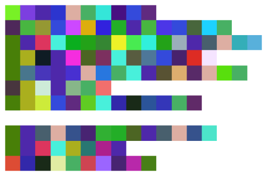
Our subword encoding method factorizes every subword-unit into $3\times 256$ values, which is reminiscent of the standard 24-bit RGB color encoding. Thus every subword can be directly visualized as one pixel with an RGB color. While this interpretation does not have any practical application, it might help to explain our method from a different angle. Note that this analogy is not perfect – our method views all indices as completely independent and thus the factorized ‘R channel’ with index $101$ is as close to $102$ as to $237$ .

We illustrate this interpretation in Figure 8, where we show the factorized subwords of the first verse and chorus of the song Suzanne by Leonard Cohen:

Suzanne takes you down to her place near the river
You can hear the boats go by, you can spend the night beside her
And you know that she’s half-crazy but that’s why you want to be there
And she feeds you tea and oranges that come all the way from China
And just when you mean to tell her that you have no love to give her
Then she gets you on her wavelength
And she lets the river answer that you’ve always been her lover

And you want to travel with her, and you want to travel blind
And you know that she will trust you
For you’ve touched her perfect body with your mind

Appendix B Full English ablation results

The full results of the comparative study from Section 4.2 (using the full set of UD metrics) are given in Table 3. This table also shows what happens if we keep a constant number of layers between the factorizer and BPE-based language models – as opposed to fixing the parameter count.

Model	# params	UPOS	XPOS	UFeats	Lemmas	UAS	LAS	MLAS	BLEX
BPE	110.8M	97.74^±0.02	97.55^±0.03	97.72^±0.04	98.03^±0.03	93.79^±0.10	92.06^±0.08	86.22^±0.11	87.94^±0.09
BPE + sampling	110.8M	97.88^±0.02	97.71^±0.05	97.82^±0.05	98.25^±0.01	93.94^±0.07	92.22^±0.05	86.44^±0.04	88.35^±0.06
BPE + sampling + averaging	110.8M	97.88^±0.04	97.72^±0.02	97.81^±0.05	98.29^±0.04	93.89^±0.13	92.22^±0.12	86.58^±0.09	88.47^±0.09
Factorizer	108.1M	97.76^±0.04	97.58^±0.04	97.74^±0.03	98.01^±0.01	94.04^±0.13	92.25^±0.13	86.26^±0.14	88.02^±0.20
Factorizer + sampling	108.1M	97.94^±0.02	97.75^±0.06	97.84^±0.06	98.40^±0.02	93.96^±0.06	92.29^±0.07	86.62^±0.11	88.71^±0.12
Factorizer + sampling + averaging	108.1M	97.97^±0.02	97.77^±0.03	97.87^±0.02	98.48^±0.03	94.06^±0.13	92.39^±0.14	86.87^±0.19	88.92^±0.19
Factorizer (12L)	86.8M	97.75^±0.02	97.54^±0.03	97.74^±0.03	98.01^±0.05	93.72^±0.08	91.93^±0.08	85.99^±0.19	87.69^±0.20
Factorizer (12L) + sampling	86.8M	97.80^±0.03	97.68^±0.04	97.72^±0.07	98.24^±0.03	93.45^±0.11	91.66^±0.08	85.46^±0.09	87.61^±0.07
Factorizer (12L) + sampling + averaging	86.8M	97.88^±0.04	97.70^±0.04	97.76^±0.04	98.31^±0.03	93.75^±0.06	92.00^±0.09	86.06^±0.20	88.19^±0.10

Table 3: Full comparison of BPE and factorizer configurations. ‘Factorizer (12L)’ denote the configuration without any additional transformer layers. The metrics are measured on the development split of en-ewt. We show the mean and standard deviation statistics over 5 random seeds, the best results are displayed in bold.

Appendix C GLUE results

As noted in the Limitations section, our method is comparable to BPE but not better on average, when evaluated on this NLU benchmark suite. The detailed results are given in Table 4.

Task	Metric	BPE	BPE	BPE	Factorizer	Factorizer	Factorizer
			+ sampling	+ sampling		+ sampling	+ sampling
				+ averaging			+ averaging
CoLA	MCC	59.56^±1.33	59.93^±1.74	60.25^±1.71	62.02^±1.82	60.71^±1.29	60.42^±2.28
MNLI	matched acc.	87.08^±0.29	86.03^±0.15	86.18^±0.07	86.35^±0.16	85.60^±0.07	85.86^±0.16
	mismatched acc.	86.48^±0.20	86.46^±0.22	86.49^±0.15	86.26^±0.11	85.61^±0.15	85.77^±0.23
MRPC	accuracy	89.61^±0.45	88.77^±0.72	88.48^±0.71	86.96^±1.18	86.96^±0.40	87.79^±1.32
	F₁	92.60^±0.45	92.00^±0.72	91.79^±0.71	90.60^±1.18	90.74^±0.40	91.27^±1.32
QNLI	accuracy	91.98^±0.22	91.93^±0.12	91.93^±0.10	92.01^±0.20	91.14^±0.22	91.58^±0.36
QPP	accuracy	91.59^±0.05	91.62^±0.11	91.63^±0.10	91.75^±0.14	91.69^±0.05	91.72^±0.07
	F₁	88.78^±0.08	88.78^±0.16	88.86^±0.13	89.04^±0.18	88.92^±0.08	88.94^±0.09
RTE	accuracy	73.14^±2.42	73.94^±1.09	75.31^±1.16	66.35^±1.41	68.88^±1.23	71.48^±1.37
SST-2	accuracy	93.60^±0.05	93.62^±0.51	93.76^±0.48	93.83^±0.41	93.07^±0.28	93.30^±0.43
STS-B	Pearson corr.	89.21^±0.34	89.26^±0.42	89.67^±0.46	89.32^±0.25	88.71^±0.10	88.84^±0.19
	Spearman corr.	89.23^±0.27	89.14^±0.33	89.52^±0.39	89.06^±0.20	88.48^±0.09	88.61^±0.20
Average		84.45^±1.00	84.43^±0.81	84.70^±0.81	83.61^±0.93	83.40^±0.66	83.90^±1.07

Table 4: Detailed development GLUE results for the English language models. We show the mean and standard deviation statistics over 5 runs with different random seeds.

Appendix D Hyperparameters

All hyperparameters are listed below: VQ-VAE hyperparameters in Table 5, pretraining hyperparameters in Table 6 and finetuning hyperparameters in Table 7. Note that the the full PyTorch (Paszke et al., 2019) source code can be found in https://github.com/ltgoslo/factorizer.

The training was performed on 128 AMD MI250X GPUs (distributed over 16 compute nodes) and took approximately 8 hours per model in a mixed precision mode.

Hyperparameter	Value
Codebook size	256
Number of codebooks	3
Number of layers	6
Hidden size	256
FF intermediate size	683
FF activation function	GEGLU
Attention heads	4
Attention head size	64
Dropout	0.1
Attention dropout	0.1
Training steps	50 000
Batch size	4 096
Warmup steps	500
Initial learning rate	0.001
Final learning rate	0.0001
Learning rate decay	cosine
Weight decay	0.01
Layer norm $\epsilon$	1e-5
Optimizer	ASAM + AdamW
ASAM $\rho$	0.2
AdamW $\epsilon$	1e-6
AdamW $\beta_{1}$	0.9
AdamW $\beta_{2}$	0.98
VQ-VAE $\beta$	0.5
Codebook EMA $\lambda$	0.96
Weight EMA $\lambda$	0.999

Table 5: VQ-VAE hyperparameters.

Hyperparameter	Value
Number of layers	12 or 15
Hidden size	768
FF intermediate size	2 048
Vocabulary size	32 768 or $3\times 256$
FF activation function	GEGLU
Attention heads	12
Attention head size	64
Dropout	0.1
Attention dropout	0.1
Training steps	31 250
Batch size	32 768 (90% steps) / 8 192 (10% steps)
Sequence length	128 (90% steps) / 512 (10% steps)
Tokens per step	4 194 304
Warmup steps	500 (1.6% steps)
Initial learning rate	0.01
Final learning rate	0.001
Learning rate decay	cosine
Weight decay	0.1
Layer norm $\epsilon$	1e-5
Optimizer	LAMB
LAMB $\epsilon$	1e-6
LAMB $\beta_{1}$	0.9
LAMB $\beta_{2}$	0.98
Gradient clipping	2.0
Factorizer $\alpha_{\textrm{split}}$ (if applicable)	0.1
Factorizer $\sigma_{\textrm{sample}}$ (if applicable)	0.0 or 0.02
BPE dropout rate (if applicable)	0.0 or 0.1

Table 6: Language model pretraining hyperparameters.

Hyperparameter	Value
Hidden size	768
Dropout	0.2
Attention dropout	0.2
Word dropout	0.15
Label smoothing	0.1
Epochs	20
Batch size	32
Warmup steps	250
Initial learning rate	0.001
Final learning rate	0.0001
Learning rate decay	cosine
Weight decay	0.001
Layer norm $\epsilon$	1e-5
Optimizer	AdamW
AdamW $\epsilon$	1e-6
AdamW $\beta_{1}$	0.9
AdamW $\beta_{2}$	0.98
Gradient clipping	10.0
Factorizer $\alpha_{\textrm{split}}$ (if applicable)	0.1
Factorizer $\sigma_{\textrm{sample}}$ (if applicable)	0.0 or 0.02
BPE dropout rate (if applicable)	0.0 or 0.1
Samples for averaging (if applicable)	128

Table 7: Hyperparameters for finetuning language models on UD treebanks.