Volcano transition in populations of phase oscillators with random nonreciprocal interactions

Abstract

Populations of heterogeneous phase oscillators with frustrated random interactions exhibit a quasi-glassy state in which the distribution of local fields is volcano-shaped. In a recent work [Phys. Rev. Lett. 120, 264102 (2018)] the volcano transition was replicated in a solvable model using a low-rank, random coupling matrix $\mathbf{M}$. We extend here that model including tunable nonreciprocal interactions, i.e. ${\mathbf{M}}^{T}\neq\mathbf{M}$. More specifically, we formulate two different solvable models. In both of them the volcano transition persists if matrix elements $M_{jk}$ and $M_{kj}$ are enough correlated. Our numerical simulations fully confirm the analytical results. To put our work in a wider context, we also investigate numerically the volcano transition in the analogous model with a full-rank random coupling matrix.

I introduction

Spin glasses are paradigmatic complex systems, whose study found application in other seemingly unrelated fields, from optimization problems to biology Mézard et al. (1987). In 1992, Daido modified the Kuramoto model of phase oscillators replacing uniform ferromagnetic-like interactions by random frustrated couplings Daido (1992), exactly as in the Sherrington-Kirkpatrick spin-glass model Sherrington and Kirkpatrick (1975); Mézard et al. (1987). The presence of frustrated interactions was expected to result in some sort of ‘oscillator glass’. It was argued in Daido (1992) that the onset of a quasi-glassy phase —characterized by algebraic relaxation and “quasientrainment”— coincided with a reconfiguration of the local fields, such that their density adopted a volcano shape (with maximal density away from zero). This conclusion was the subject of some controversy Stiller and Radons (1998); Daido (2000); Stiller and Radons (2000), see also Sec. IV.B.1. of Acebrón et al. (2005). However, recent numerical simulations by Kimoto and Uezu Kimoto and Uezu (2019) provided additional support to the glassy nature of the volcano phase by measuring a suitably defined spin-glass order parameter.

In parallel to the previous works, phase oscillator ensembles endowed with low-rank random coupling matrices have been studied Bonilla et al. (1993); Kloumann et al. (2014); Uezu et al. (2015); Ottino-Löffler and Strogatz (2018), with the expectation that they reproduce features of the original full-rank-disordered system Daido (1992). In particular, Ottino-Löffler and Strogatz Ottino-Löffler and Strogatz (2018) replicated the volcano transition with associative-memory-type interactions. In contrast to the original setup Daido (1992), the model in Ottino-Löffler and Strogatz (2018) does not display algebraic relaxation dynamics typical of spin glasses, but it has the advantage of being analytically solvable. A similar model had been previously analyzed with a completely different approach by Uezu and coworkers Uezu et al. (2015), exploiting a theoretical link between the oscillator population and the classical XY model. The results in Uezu et al. (2015) and Ottino-Löffler and Strogatz (2018) are complementary and mutually consistent; still, the approach in Ottino-Löffler and Strogatz (2018) has the advantage of making stability analysis possible.

In real spin glasses, as well as in the Daido model Daido (1992), the interactions are symmetric, i.e. reciprocal. However, nonreciprocal interactions are found almost everywhere, from aggregates of neurons to self-motile active particles, see e.g. Fruchart et al. (2021). Populations of phase oscillators with asymmetric couplings are found in models inspired in neuroscience Montbrió and Pazó (2018); Laing et al. (2021), society Hong and Strogatz (2011), hydrodynamically coupled flagella Uchida and Golestanian (2010), etc. The effect of nonreciprocity on glassy phases in the context of synchronization is attracting attention Hanai (2022) but remains scarcely explored; particularly in comparison to random neural networks, see e.g. the discussion in Martí et al. (2018); Berlemont and Mongillo (2022) and references therein. Remarkably, incorporating asymmetric couplings in the Daido model has only been undertaken by Stiller and Radons in Stiller and Radons (1998). In this work it was concluded that the quasi-glassy phase did not persist if the random interactions were not reciprocal enough (in statistical sense). Still, it is important to stress that what is called quasi-glassy in Stiller and Radons (1998) differs from the state emerging at the volcano transition in Daido (1992). Revisiting these questions appears to be in order, specially considering the current computational power.

In this paper we put forward two solvable models of populations of oscillators with low-ranked, asymmetric, random interactions. Specifically, we generalize the model in Ottino-Löffler and Strogatz (2018) by introducing a free parameter $\eta\in[-1,1]$, which allows us to continuously interpolate between fully symmetric ($\eta=1$) and fully antisymmetric interactions ($\eta=-1$), going over the uncorrelated case ($\eta=0$). This new ingredient does not degrade the tractability of the models. Moreover, we refine the analysis in Ottino-Löffler and Strogatz (2018) and allow the frequency distribution to be any unimodal symmetric distribution (not only Lorentzian). Surprisingly, in spite of the similarities of the models introduced here, their phase diagrams turn out to be notably different. For comparison purposes, we carry out simulations with the equivalent model with a full-rank random coupling matrix Stiller and Radons (1998). We find that the volcano transition is only possible above a critical level of reciprocity, different from the low-rank models. Perhaps the main message of this work is the impossibility of extrapolating the quantitative results from low-rank to full-rank structural disorder, refuting a conjecture raised in Ottino-Löffler and Strogatz (2018).

This article is organized as follows. In Sec. II we introduce the two models of populations of phase oscillators with low-rank asymmetric coupling matrix. Section III is devoted to the numerical study of the volcano transition in both models. The results are theoretically described in Sec. IV. Section V presents a numerical study of the volcano transition for full-rank structural disorder with reciprocal and nonreciprocal interactions. Finally, Sec. VI summarizes the main conclusions of this work.

II Models with low-rank coupling matrix

We investigate a population of heterogeneous phase oscillators with quenched random couplings:

$${\dot{\theta}}_{j}=\omega_{j}+\frac{J}{N}\sum_{k=1}^{N}M_{jk}\sin(\theta_{k}-\theta_{j}).$$ (1)

The phases $\theta_{j}$ are cyclic variables, and the population size is $N\gg 1$. The natural frequencies $\{\omega_{j}\}_{j=1,\ldots,N}$ are drawn from a symmetric unimodal distribution $g(\omega)$, which is assumed to be centered at zero without lack of generality (by going to a rotating frame if necessary). In Eq. (1), matrix elements $M_{jk}$ codify the competition between synchronizing ($M_{jk}>0$) and anti-synchronizing ($M_{jk}<0$) interactions. Moreover, we include a global coupling constant $J>0$.

In Ottino-Löffler and Strogatz (2018) the coupling matrix ${\mathbf{M}}$ was constrained to be symmetric. Here we introduce a parameter $\eta$ controlling the weight in ${\mathbf{M}}$ of the symmetric and the antisymmetric matrices, ${\mathbf{S}}$ and ${\mathbf{A}}$, respectively. We have therefore:

$${\mathbf{M}}=\frac{1}{2}\left[(1+\eta){\mathbf{S}}+(1-\eta){\mathbf{A}}\right]\,.$$ (2)

We allow parameter $\eta$ to vary in the range $[-1,1]$. The symmetric situation is recovered for $\eta=1$.

II.1 Model 1

The first model we propose assumes that each oscillator has two associated $L$-dimensional connectivity vectors ${\bf u}_{j}$ and ${\bf v}_{j}$, with quenched random components equal to $\pm 1$: ${\bf u}_{j},{\bf v}_{j}\in\{\pm 1\}^{L}$. The elements of the symmetric ($\mathbf{S}$) and antisymmetric ($\mathbf{A}$) matrices are computed from scalar products of the interaction vectors:

$$S_{jk} = {\bf u}_{j}\cdot{\bf u}_{k}-{\bf v}_{j}\cdot{\bf v}_{k}\,,$$ (3a)

$$A_{jk} = {\bf u}_{j}\cdot{\bf v}_{k}-{\bf v}_{j}\cdot{\bf u}_{k}\,.$$ (3b)

Note that, with this formulation, self-interactions are automatically excluded: $S_{jj}=A_{jj}=0$. Matrix $\bf S$ yields the coupling type already used in Ottino-Löffler and Strogatz (2018) (with a slightly different definition), while $\bf A$ codifies an anti-reciprocal interaction.

The statistical properties of offdiagonal elements of the coupling matrix are summarized next. First of all, the mean is zero ($\langle M_{jk}\rangle=0$). The variance is

$$\langle M_{jk}^{2}\rangle=L(1+\eta^{2})\,.$$ (4)

The correlation coefficient between mirror elements above and below the main diagonal of ${\mathbf{M}}$ is

$$\mbox{corr}(M_{jk},M_{kj})=\frac{\langle M_{jk}M_{kj}\rangle}{\langle M_{jk}^{2}\rangle}=\frac{2\eta}{1+\eta^{2}}\,.$$ (5)

The correlation vanishes at $\eta=0$, while maximal (anti)correlation is achieved at $\eta=1$ ($-1$).

The rank of matrix $\mathbf{M}$ is $2L$, save for $\eta=0$ . For the sake of analytical tractability, we assume low-ranked disorder, mathematically expressed by the condition $L\ll\log_{2}N$. This key assumption permits us to use the Ott-Antonsen ansatz Ott and Antonsen (2008), as in Ottino-Löffler and Strogatz (2018).

II.2 Model 2

Our second model is similar to model 1, but with independent interaction vectors for matrix $\mathbf{A}$. In this way we have:

$$S_{jk} = {\bf u}_{j}\cdot{\bf u}_{k}-{\bf v}_{j}\cdot{\bf v}_{k}\,,$$ (6a)

$$A_{jk} = \tilde{\bf u}_{j}\cdot\tilde{\bf v}_{k}-\tilde{\bf v}_{j}\cdot\tilde{\bf u}_{k}\,.$$ (6b)

This means that each oscillator is characterized by its frequency $\omega_{j}$ and four $L$-dimensional vectors (${\bf u}_{j},{\bf v}_{j},\tilde{\bf u}_{j},\tilde{\bf v}_{j}$). Variance and correlation in Eqs. (4) and (5) also hold for model 2. Now, however, matrices $\bf S$ and $\bf A$ are statistically independent. The rank of matrix $M$ is $4L$, save for $\eta=\pm 1$ where it equals $2L$.

III Numerical Results

In our simulations we adopt a Gaussian probability density function for the natural frequencies:

$$g(\omega)=\frac{e^{-\frac{\omega^{2}}{2\sigma^{2}}}}{\sigma\sqrt{2\pi}}.$$

The value of the standard deviation $\sigma$ can be arbitrarily selected by rescaling time and the coupling constant $J$ in Eq. (1). We adopt $\sigma=\sqrt{\pi/2}$ for the numerical simulations. Throughout this paper the numerical integration of the ordinary differential equations is performed using the fourth-order Runge-Kutta method with time step 0.1 t.u.

Figure 1: Phase portraits of the local fields $P_{j}(t)$ below and above the volcano transition: (a) $J=3.5$, and (b) $J=4.5$. In graph (c) we show the radial distributions of local fields for the previous values of $J$ together with an intermediate value ($J=4$).

III.1 Model 1

We start considering model 1. For fixed $\sigma$, our system depends on four free parameters: $N$ (the population size), $L$ (the dimension of the interaction vectors $\mathbf{u}$ and $\mathbf{v}$), $J$ (the coupling constant), and $\eta$ (the asymmetry parameter). We are interested in the large-$N$ behavior, such that only a marginal dependence upon the realization of frequencies and connections is expected. The effect of the remaining parameters $L$, $J$ and $\eta$ is investigated hereafter.

Similar to the spin-glass transition, the emergence of the volcano phase cannot be detected measuring a global order parameter. It remains near zero below and above the critical point. Instead, it is the distribution of complex local fields

$$P_{j}(t)\equiv r_{j}e^{i\psi_{j}}=\frac{1}{N}\sum_{k=1}^{N}M_{jk}e^{i\theta_{k}}\,,$$ (7)

what undergoes a structural change, see below. For later use it is convenient to rewrite Eq. (1) in terms of the local fields:

$${\dot{\theta}}_{j}=\omega_{j}+Jr_{j}\sin(\psi_{j}-\theta_{j})\,.$$ (8)

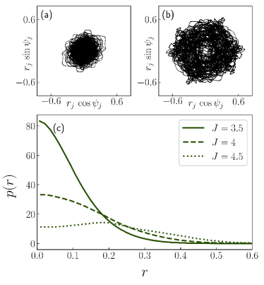
Our first numerical simulation, in Figs. 1(a) and 1(b), show the phase portraits of the local fields $P_{j}(t)$ for a population of $N=500$ oscillators interacting nonreciprocally with asymmetry parameter $\eta=1/4$ and $L=3$. Figures 1(a) and 1(b) correspond to values of $J$ below and above the volcano transition, respectively. In the former plot the density of local fields is maximal at the origin, while in Fig. 1(b) the volcano shape is apparent. Figure 1(c) depicts the radial distributions of local fields for the same values of $J$ as in Figs. 1(a) and 1(b), plus an intermediate $J$ value near the critical value $J_{v}$. At the volcano transition the radial distribution of the local fields $p(r)$ changes from concave down at the origin to concave up. This means that $p(r)$ peaks at $r_{*}>0$ for $J>J_{v}$.

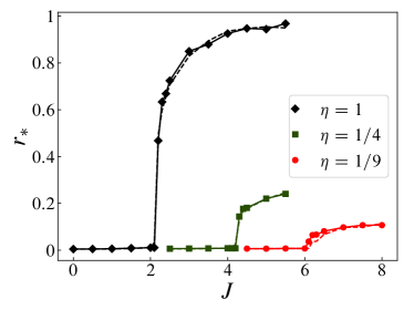
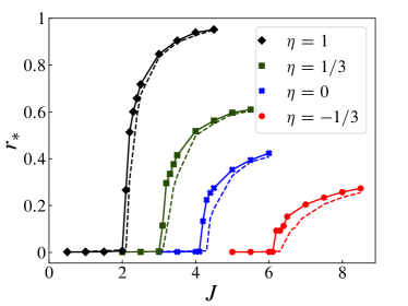
Next, we investigate the dependence of $r_{*}$ on the coupling constant $J$. Three values of $\eta\in\{1,1/4,1/9\}$ were selected. In addition, for each of them two different values of the vector dimension $L\in\{2,3\}$ were chosen. Figure 2 presents the results. The peak radius $r_{*}$ departs from zero above the $\eta$-dependent critical coupling $J_{v}(\eta)$. Notably, $J_{v}$ increases as $\eta$ is lowered, i.e. as the correlation between mirror entries of the connectivity matrix decreases. Moreover, $r_{*}$ attains significantly smaller values as $\eta$ is lowered, i.e. the “volcano width” decreases as the interactions become less reciprocal. Eventually, no transition is found for $\eta\leq 0$. This means that the volcano transition requires positive correlations between $M_{jk}$ and $M_{kj}$ to occur. It is also interesting to note that the results are apparently insensitive to the size $L$ of the connectivity vectors, as already pointed out in Ottino-Löffler and Strogatz (2018) for $\eta=1$. Actually, the irrelevance of $L$ only holds provided that $2^{2L}\ll N$, as theoretically justified in Sec. IV.

Figure 2: Position of the maximum in the radial distribution of local fields as a function of the coupling constant $J$ for model 1 with $N=500$ oscillators. Data sets correspond to three different values of $\eta\in\{1,1/4,1/9\}$. For each $\eta$ value two different connectivity-vector sizes were selected: $L=2$ (filled symbols connected by a solid line) and $L=3$ (empty symbols, dashed line). Each point represents the location of the maximum in the histogram of the local-field amplitudes, collected from 100 realizations of random frequencies and connectivity vectors. For each simulation the system was integrated for $500$ t.u., after a transient of $300$ t.u.

III.2 Model 2

Our numerical study of model 2 proceeded analogously to model 1. As above, we tracked the peak value $r_{*}$ as a function of the coupling constant $J$, for different values of $\eta$ and $L$. The results for $N=1000$ are shown in Fig. 3. As with model 1, the smaller $\eta$ the larger the critical coupling $J_{v}$. To our surprise, the volcano transition also occurs for negative $\eta$ values, i.e. when the inwards and the outwards connections are statistically anticorrelated. When $L$ is changed from $1$ to $4$, a small displacement of the values of $J_{v}(\eta)$ is observed in the figure. We argue in the next section that $J_{v}$ is insensitive to the value of $L$, provided that $2^{4L}\ll N$, This does not hold at all for $L=4$ ($2^{16}\approx 6.5\times 10^{4}$), but nevertheless the displacement of $J_{v}$ in this case remains quite moderate.

Figure 3: Position of the maximum in the radial distribution of local fields as a function of the coupling constant $J$ for model 2 with $N=1000$ oscillators. Data sets correspond to four different values of $\eta\in\{-1/3,0,1/3,1\}$. For each $\eta$ value simulations adopted two different connectivity-vector sizes: $L=1$ (filled symbols connected by solid lines) and $L=4$ (empty symbols, dashed lines).

IV Theoretical Analysis

The theoretical analysis is similar for models 1 and 2. In both cases we adopt the thermodynamic limit $N\to\infty$, such that the state of the system is described by a phase density $\rho$.

IV.1 Model 1

We start presenting the theory for model 1, and defer the relevant modifications for model 2 to the end of this section. To lighten the notation we introduce a $2L$-dimensional vector $\bf w$, which is the concatenation of the interaction vectors $\bf u$ and $\bf v$: ${\bf w}=({\bf u}^{T},{\bf v}^{T})^{T}$. Adopting this notation, we have that $\rho(\theta|\omega,\mathbf{w};t)d\theta$ is the fraction of oscillators with phases between $\theta$ and $\theta+d\theta$ at time $t$ with natural frequency $\omega$ and interaction vector $\bf w$.

The density obeys the continuity equation:

$$\partial_{t}\rho+\partial_{\theta}(v\rho)=0.$$ (9)

Here, recalling Eq. (8), we use $v$ as a short-hand notation for the velocity:

$$v(\theta,\omega,{\bf w},t)=\omega+J\,\mathrm{Im}[P({\bf w},t)e^{-i\theta}]\,.$$ (10)

The local field $P$, see Eq. (7), is simply the double average of $e^{i\theta}$ over $2^{2L}$ different interaction vectors and over the continuum of natural frequencies:

$$P({\bf w},t)=\\ \frac{1}{2^{2L}}\sum_{\bf w^{\prime}}{\cal{M}}({\bf w},{\bf w}^{\prime})\int_{-\infty}^{\infty}d\omega\,g(\omega)\int_{0}^{2\pi}\rho(\theta|\omega,{\bf w}^{\prime};t)e^{i\theta}d\theta.$$ (11)

Matrix $\bm{\mathcal{M}}$ has dimension $2^{2L}\times 2^{2L}$, and its elements are calculated as those of ${\mathbf{M}}$, see Eq. (2). Each row (column) corresponds to a different binary string $\bf w$ (${\bf w}^{\prime}$), hence the matrix dimension. (We define $2^{2L}\times 2^{2L}$ matrices ${\bm{\mathcal{S}}}$ and ${\bm{\mathcal{A}}}$ from Eq. (3) analogously.) The dependence of $v$ on $\rho$ via $P$ confers nonlinearity to the continuity Eq. (9).

The key point of the analysis it the fact that, as Eq. (10) only depends on the first harmonic in $\theta$, we can apply the Ott-Antonsen ansatz Ott and Antonsen (2008):

$$\rho(\theta|\omega,{\bf w};t)=\frac{1}{2\pi}\left[1+\sum_{n=1}^{\infty}\alpha(\omega,{\bf w},t)^{n}e^{in\theta}+\mbox{c.c.}\right]\,.$$ (12)

Here, $\alpha$ is the coefficient of the first harmonic, and c.c. stands for complex conjugate. Inserting the previous expansion into the continuity equation (9), we obtain the evolution equation for $\alpha$:

$$\partial_{t}\alpha(\omega,{\bf w},t)=-i\omega\alpha+\frac{J}{2}\left[P^{*}-P\alpha^{2}\right].$$ (13)

Moreover, assuming the Ott-Antonsen ansatz (12), the equation for the local field (11) simplifies:

$$P({\bf w},t)=\frac{1}{2^{2L}}\sum_{{\bf w}^{\prime}}{\cal M}({\bf w},{\bf w}^{\prime})\int d\omega\,g(\omega)\alpha(\omega,{\bf w}^{\prime},t)^{*}.$$ (14)

Plugging this expression into Eq. (13), we get a closed vector integro-differential equation.

We analyze next the stability of the incoherent state $\alpha=0$ against infinitesimal perturbations. Therefore we drop the nonlinear term in Eq. (13). For the resulting linear system, we take an exponential ansatz $\alpha(\omega,{\bf w},t)=\beta(\omega,{\bf w})e^{\lambda t}$. This yields an equation for the exponential growth rate $\lambda$:

$$(\lambda+i\omega)\beta(\omega,{\bf w})=\frac{J}{2^{2L+1}}\sum_{{\bf w}^{\prime}}{\cal M}({\bf w},{\bf w}^{\prime})b({\bf w}^{\prime}),$$ (15)

where we have introduced the shorthand notation $b({\bf w})\equiv\int d\omega g(\omega)\beta(\omega,{\bf w})$. Reordering terms, and integrating over $\omega$ both sides of the equation, we get:

$$b({\bf w})=\frac{J}{2^{2L+1}}\int_{-\infty}^{\infty}\frac{g(\omega)}{\lambda+i\omega}d\omega\sum_{{\bf w}^{\prime}}{\cal M}({\bf w},{\bf w}^{\prime})b({\bf w}^{\prime})$$ (16)

At the critical coupling $J_{v}$, the real part of the eigenvalue $\lambda=\lambda_{r}+i\Omega$ approaches zero: $\lambda_{r}\to 0^{+}$. Hence, the previous equation at criticality becomes (written in matrix form):

$$\left(c\frac{J_{v}}{2^{2L+1}}{\bm{\mathcal{M}}}-{\bm{\mathcal{I}}}\right){\mathbf{b}}=0,$$ (17)

where $c\equiv\pi g(-\Omega)-i\int g(\omega-\Omega)/\omega\,d\omega$, and ${\bm{\mathcal{I}}}$ is the identity matrix. Nontrivial solutions (${\mathbf{b}}\neq{\mathbf{0}}$) of the linear equation (17) are eigenvectors of $\bm{\mathcal{M}}$ corresponding to nonzero eigenvalues.

Computing the eigenvalues of $\bm{\mathcal{M}}$ is surprisingly simple. We find that ${\bm{\mathcal{M}}}^{2}=\eta{\bm{\mathcal{S}}}^{2}$, by virtue of the identities ${\bm{\mathcal{S}}}^{2}+{\bm{\mathcal{A}}}^{2}={\bm{\mathcal{SA}}}+{\bm{\mathcal{AS}}}=0$, which are easily proven. Therefore, all we need is the eigenvalue spectrum of ${\bm{\mathcal{S}}}$. As found in Ottino-Löffler and Strogatz (2018), the nonzero eigenvalues are $2^{2L}$ and $-2^{2L}$, both of them with multiplicity $L$. Hence, the nonzero eigenvalues of ${\bm{\mathcal{M}}}$ are simply $\pm\sqrt{\eta}\,2^{2L}$. For $\eta<0$ the nontrivial eigenvalues are purely imaginary, and no solution of Eq. $\eqref{cjmib}$ exists since $\mathrm{Re}(c)\neq 0$, i.e. there is not a critical $J_{v}$ value. For $\eta>0$, matrix ${\bm{\mathcal{M}}}$ possesses real eigenvalues and Eq. (17) may only hold provided $\mathrm{Im}(c)=0$. If $g(\omega)$ is an even unimodal function, then $\Omega=0$ necessarily. In turn, $c=\pi g(0)$, and the critical coupling turns out to be:

$$J_{v}^{(1)}=\frac{1}{\sqrt{\eta}}\times\frac{2}{\pi g(0)}.$$ (18)

We have included the superscript $(1)$ to emphasize the result refers to model 1. Equation (18) should provide an accurate estimation of $J_{v}$ for large ensembles of oscillators, if the condition $N\gg 2^{2L}$ is fulfilled. This condition is tantamount to assuming that a large number of oscillators share each of the possible interaction vectors ${\bf w}$, such that the continuous formulation is meaningful. Let us confront Eq. (18) with the result of the numerical simulations condensed in Fig. 2. For a frequency dispersion $\sigma=\sqrt{\pi/2}$, Eq. (18) becomes $J_{v}=2/\sqrt{\eta}$. In particular, for the values $\eta$ selected in Fig. 2, the predicted critical couplings are $J_{v}=2$, $4$, and $6$, irrespective of $L$. We observe an excellent agreement between theory and simulations.

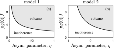
We end the analysis of model 1 showing its phase diagram in Fig. 4(a). Notice the divergence of the volcano phase boundary as $\eta\to 0^{+}$, i.e. as the correlation between inward and outward links vanishes.

Figure 4: Phase diagrams of models 1 (a) and 2 (b) for symmetric unimodal frequency distribution. The boundaries of the volcano phase in panels (a) and (b) are defined by Eqs. (18) and (21), respectively. Note the different range of $\eta$ in each panel.

IV.2 Model 2

The theoretical analysis of model 2 is analogous to the one for model 1 above. Therefore, we only indicate the key differences. We have now four $L$-dimensional vectors associated with each oscillator. In turn, the dimensionality of matrix $\bm{\mathcal{M}}$ is $2^{4L}\times 2^{4L}$, as there are $2^{4L}$ different combinations of $\bf u$, $\bf v$, $\tilde{\bf u}$ and $\tilde{\bf v}$. The mathematical relation between $\bm{\mathcal{M}}$ and the $2^{2L}\times 2^{2L}$ matrices $\bm{\mathcal{S}}$ and $\bm{\mathcal{A}}$ is not trivial at first sight. It can be conveniently expressed with the Kronecker product, denoted by $\otimes$:

$$\bm{\mathcal{M}}=\frac{1}{2}\left[(1+\eta)\bm{\mathcal{E}}\otimes\bm{\mathcal{S}}+(1-\eta)\bm{\mathcal{A}}\otimes\bm{\mathcal{E}}\right],$$ (19)

where $\bm{\mathcal{E}}$ is a $2^{2L}\times 2^{2L}$ matrix of ones.

Eventually, the analysis leads to a marginality condition analogous to Eq. (17):

$$\left(c\frac{J_{v}}{2^{4L+1}}{\bm{\mathcal{M}}}-{\bm{\mathcal{I}}}\right){\mathbf{b}}=0\,,$$ (20)

where ${\bm{\mathcal{I}}}$ is the $2^{4L}\times 2^{4L}$ identity matrix. The critical coupling is dictated by the eigenvalue of ${\bm{\mathcal{M}}}$ with the largest real part. Therefore, the problem reduces to finding the eigenvalue spectrum of ${\bm{\mathcal{M}}}$.

Firstly, let us note that $\bm{\mathcal{E}}\otimes\bm{\mathcal{S}}$ commutes with $\bm{\mathcal{A}}\otimes\bm{\mathcal{E}}$, implying they share a common basis of eigenvectors. The proof follows: $({\bm{\mathcal{E}}}\otimes{\bm{\mathcal{S}}})(\bm{\mathcal{A}}\otimes\bm{\mathcal{E}})-(\bm{\mathcal{A}}\otimes\bm{\mathcal{E}})(\bm{\mathcal{E}}\otimes\bm{\mathcal{S}})=\bm{\mathcal{EA}}\otimes\bm{\mathcal{SE}}-\bm{\mathcal{AE}}\otimes\bm{\mathcal{ES}}=0$, where we have used that $\bm{\mathcal{E}}$ commutes with $\bm{\mathcal{S}}$ and $\bm{\mathcal{A}}$ in the last identity.

At this point we notice that ${\bm{\mathcal{E}}}$ possesses only one nonzero eigenvalue $2^{2L}$, with associated eigenvector ${\bf e}_{1}=(1,1,\ldots,1)^{T}$. Hence, the relevant eigenvectors of ${\bm{\mathcal{M}}}$ have the form ${\mathbf{e}}_{1}\otimes\bm{\mathbf{s}}_{i}$ or ${\mathbf{a}}_{i}\otimes\bm{\mathbf{e}}_{1}$, where $\{{\mathbf{s}}_{i}\}$ and $\{{\mathbf{a}}_{i}\}$ are the eigenvector sets corresponding to nonzero eigenvalues of $\bm{\mathcal{S}}$ and $\bm{\mathcal{A}}$, respectively. Other combinations of eigenvectors yield null eigenvalues; note in particular that $\bm{\mathcal{E}}{\mathbf{s}}_{i}=0$, because the ${\mathbf{s}}_{i}$’s are orthogonal to ${\mathbf{e}}_{1}$. Likewise, $\bm{\mathcal{E}}{\mathbf{a}}_{i}=0$.

Following our previous discussion, the eigenvalue spectrum of ${\bm{\mathcal{M}}}$ is easily obtained. Nonzero eigenvalues come from either term of $\bm{\mathcal{M}}$, see Eq. (19), by virtue of the identities $\bm{\mathcal{S}}\mathbf{e}_{1}=\bm{\mathcal{A}}\mathbf{e}_{1}=\mathbf{0}$. (Matrices $\bm{\mathcal{S}}$ and $\bm{\mathcal{A}}$ have zero row sum.) Eigenvalues corresponding to the eigenvectors ${\mathbf{a}}_{i}\otimes\bm{\mathbf{e}}_{1}$ are pure imaginary, since $\bm{\mathcal{A}}$ is a skew-symmetric matrix. Their exact values are therefore immaterial for this problem . The other nonzero eigenvalues of ${\bm{\mathcal{M}}}$, corresponding to eigenvectors ${\mathbf{e}}_{1}\otimes\bm{\mathbf{s}}_{i}$, are real. Their values are $\pm(1+\eta)2^{4L-1}$, since we know $\bm{\mathcal{S}}{\mathbf{s}}_{i}={\pm}2^{2L}{\mathbf{s}}_{i}$ from Ottino-Löffler and Strogatz (2018). The critical coupling is obtained by considering the positive eigenvalue of $\bm{\mathcal{M}}$ in Eq. (20):

$$J_{v}^{(2)}=\frac{4}{1+\eta}\times\frac{1}{\pi g(0)}$$ (21)

This equation accurately predicts the volcano transition in our simulations in Fig. 3: For the four values of $\eta$ selected ($1$, $1/3$, $0$, and $-1/3$), Eq. (21) predicts $J_{v}=2$, $3$, $4$, and $6$.

Equation (21) allows us to represent the phase diagram in Fig. 4(b). Remarkably, the divergence of $J_{v}$ is now located at $\eta_{\infty}=-1$, contrasting with $\eta_{\infty}=0$ in model 1. This discrepancy implies that the correlation between $M_{jk}$ and $M_{kj}$ is not enough to determine the value of $\eta_{\infty}$. The key difference between models 1 and 2 is that the symmetric and antisymmetric matrices $\mathbf{S}$ and $\mathbf{A}$ —contributing to $\mathbf{M}$— are independent for model 2, but not for model 1.

IV.3 Model 1+2

We conclude the theoretical analysis noticing that models 1 and 2 can be combined to create a continuum of solvable models, with two antisymmetric components weighted by parameter $\beta$:

$$A_{jk}=(1-\beta)[{\bf u}_{j}\cdot{\bf v}_{k}-{\bf v}_{j}\cdot{\bf u}_{k}]+\beta[\tilde{\bf u}_{j}\cdot\tilde{\bf v}_{k}-\tilde{\bf v}_{j}\cdot\tilde{\bf u}_{k}]$$ (22)

This model remains analytically tractable with critical coupling

$$J_{v}=\frac{4}{\sqrt{4\eta+(2\beta-\beta^{2})(1-\eta)^{2}}}\times\frac{1}{\pi g(0)}\,.$$ (23)

The divergence of $J_{v}$ occurs at $\eta_{\infty}=\beta/(\beta-2)$.

V Model with full-rank coupling matrix

In this section we investigate to what extent our previous results carry over to the original model with a full-rank coupling matrix Daido (1992); Stiller and Radons (1998); Kimoto and Uezu (2019). Such a possibility was already explored in Ottino-Löffler and Strogatz (2018) for reciprocal coupling and Lorentzian $g(\omega)$ with an inconclusive answer.

The “full-rank model” writes:

$${\dot{\theta}}_{j}=\omega_{j}+\frac{\tilde{J}}{\sqrt{N}}\sum_{k=1}^{N}J_{jk}\sin(\theta_{k}-\theta_{j})\,.$$ (24)

Nondiagonal elements of the coupling matrix $\mathbf{J}$ are drawn from a zero-mean, unit-variance Gaussian distribution. Note the prefactor $N^{-1/2}$, instead of $N^{-1}$ as in (1). The correlation between symmetric elements ($j\neq k$) is:

$$\langle J_{jk}J_{kj}\rangle=\tau\,.$$ (25)

As above, we focus on the radial density of the local fields, which are

$$r_{j}e^{i\Psi_{j}}=\frac{1}{\sqrt{N}}\sum_{k}J_{jk}e^{i\theta_{k}}\,.$$

V.1 Reciprocal coupling, $\tau=1$

We start with the symmetric case ($\tau=1$), originally considered in Daido (1992), and recently revisited in Kimoto and Uezu (2019). In the latter work an analytical value of $\tilde{J}_{v}$ was proposed based on a mapping between model (24) with Gaussian $g(\omega)$ and the classical XY model at finite temperature.

The thermodynamic limit of model (24) coincides with our model in Eq. (1) adopting $L=N/2\to\infty$, since the binomial-distributed matrix elements become Gaussian distributed (central limit theorem). As done in Ottino-Löffler and Strogatz (2018), it is worth extrapolating our analytical result in Eq. (18), setting $\eta=1$, to the full-rank model (24), even if it is out of its range of validity. The extrapolated critical coupling turns out to be quite simple:

$$\tilde{J}_{v}=\frac{2}{\pi g(0)}\,.$$ (26)

Remarkably, if we particularize this result for Gaussian $g(\omega)$ the value of $\tilde{J}_{v}$ coincides with the one theorized in Ref. Kimoto and Uezu (2019). The latter reference exploited a mapping between the saddle-point equations of the classical XY model at finite temperature and the model in Eq. (24) with Gaussian $g(\omega)$. Still, the numerical verification of the result in Kimoto and Uezu (2019) was not straightforward. The numerical procedure involved decreasing the frequency dispersion quasi-adiabatically.

Figure 5: Volcano transition in the model defined by Eq. (24) for $\tau=1$ and $N=400$. Red circles and blue squares indicate the position of the maximum in the radial distribution of local fields $r_{*}$, for two different protocols: increasing $\tilde{J}$ quasi-adiabatically (see text), and with random initial phases for each $\tilde{J}$ value. The exact value of $r_{*}$ for each $\tilde{J}$ value is determined fitting the histogram values. Inset: Empirical radial distribution of local fields for $\tilde{J}=2$. The red curve is the biparametric fitting function in Eq. (27).

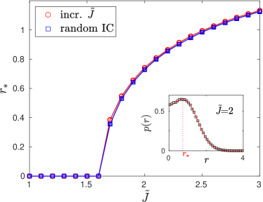
To shed more light on this issue, we decided to implement the simulation ourselves. Instead of slowly decreasing $\sigma$ as in Kimoto and Uezu (2019), we kept $\sigma=\sqrt{\pi/2}$ slowly increasing $\tilde{J}$ from 0. Both procedures should be almost equivalent if the increments in $\tilde{J}$ are small enough and transients are long enough. In our case, we implemented steps of size $\Delta\tilde{J}=10^{-3}$, and integrations $10^{3}$ t.u. long for each $\tilde{J}$ value. At particular values of $\tilde{J}$ the system was integrated for $5\times 10^{3}$ t.u. saving the local fields every time unit. This procedure was repeated 20 times, each with an independent sampling of natural frequencies and coupling matrix elements in order to achieve good statistics. The behavior of the peak value $r_{*}$ for $N=400$ is shown in Fig. 5 (virtually the same result is obtained for $N=200$). In the figure the red circles are the maxima of the fitting function used to smooth the histogram. For each $\tilde{J}$ value, the histogram was fitted by the normalized two-parametric function

$$p(r)=C\,\{\exp[-(r-\mu)^{2}/\xi]+\exp[-(r+\mu)^{2}/\xi]\}\,,$$ (27)

where $C(\mu,\xi)$ is the normalization constant: $\int_{0}^{\infty}p(r)rdr=1$. The form of $p(r)$ is suggested by the solution for $\tilde{J}=0$: $\mu=0$, $\xi=1$, and Ref. Ottino-Löffler and Strogatz (2018). The goodness of the fittings is excellent for all $\tilde{J}$ values. This is illustrated, for $\tilde{J}=2$, by the inset in Fig. 5. From the fitting line, the condition $p^{\prime}(r_{*})=0$, allows to obtain the maximum as the nontrivial solution of $e^{4\mu r_{*}/\xi}(\mu-r_{*})-\mu-r_{*}=0$. The results in Fig. 5 show a critical point clearly below the value $\tilde{J}=2$, predicted by Eq. (26). Thus our result aligns with the work by Daido Daido (1992), under appropriate rescalings, but not with Ref. Kimoto and Uezu (2019).

The discrepancy with the result in Kimoto and Uezu (2019) is intriguing. The theoretical treatment in Kimoto and Uezu (2019) is not completely rigorous, specially concerning the drifting oscillators, whose contribution is neglected. Regarding the numerical procedure in Kimoto and Uezu (2019), the results are obtained from one realization of the model, not from an ensemble of realizations. As a final effort to improve our understanding, we decided to redo the simulation in Kimoto and Uezu (2019). The frequencies were sampled once and their dispersion was progressively decreased, keeping the coupling matrix elements $J_{jk}$ and the coupling constant ($\tilde{J}=1$) fixed. Our result, for one single realization as in Kimoto and Uezu (2019), is a critical dispersion $\sigma_{v}$ closer to our inference from the empirical value of ${\tilde{J}}_{v}$ in Fig. 5 ($\sigma_{v}=\sqrt{\pi/2}/{\tilde{J}}_{v}$) than to the prediction from Eq. (26) ($\sigma_{v}=\sqrt{\pi/8}$), see the Supplmental Material . Whatever the correct interpretation of these results is, it is clear that the model with full-rank disorder is truly more complex than the models with low-rank disorder.

V.2 Nonreciprocal coupling, $\tau<1$

Next, we consider the model defined by Eq. (24) with nonreciprocal interactions, i.e. $\tau<1$. In Stiller and Radons (1998) this model was investigated, putting the focus on a static phase —at large coupling— in which all the oscillators are frozen in random positions (in a certain rotating frame). Such state was identified with the spin glass (in disagreement with Daido (1992); Kimoto and Uezu (2019)). We focus here on the volcano transition, without investigating the dynamics further. We anticipate that the static phase found in Stiller and Radons (1998) falls inside the volcano phase, see below.

Figure 6: Empirical phase diagram of model (24) with $N=400$ oscillators, and Gaussian frequency distribution of variance $\pi/2$. Triangles correspond to empirical critical couplings of the volcano transition $\tilde{J}_{v}$, at particular values of the correlation $\tau$. To determine $\tilde{J}_{v}$, the values of $\tilde{J}$ were sampled with a spacing of 0.1. The amplitudes of the local fields were collected from 100 independent realizations, each run for 1000 t.u. after a transient of 2000 t.u. and random initial phases. The resulting histograms of local fields radii were fitted to Eq. (27). As a guide to the eye we depict a dashed line, obtained fitting the critical couplings to the function $\tilde{J}_{v}(\tau)=a/(\tau-\tau_{\infty})^{\gamma}$; $\tau_{\infty}=0.1938$, $\gamma=0.542$, $a=1.481$.

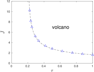
Our initial numerical simulations for $\tau=1/4$ did not reveal any difference between increasing $J$ quasiadiabatically or setting random initial conditions (not shown), as occurred with $\tau=1$. Hence, we decided to estimate the critical coupling $\tilde{J}_{v}(\tau)$ taking random initial conditions, irrespective of the value of $\tau$. Figure 6 summarizes our results. Triangles mark the location of the volcano transition at different $\tau$ values. The data are fitted to a simple algebraic formula, suggesting a divergence of $\tilde{J}_{v}$ at at a critical $\tau$ value around 0.19, see figure caption.

Our two models with low-rank disorder and the model with full-rank disorder have in common that the critical coupling increases as reciprocity is decreased. At the same time, we observed that the “volcano width” decreases as reciprocity diminishes in all cases. However, the divergence of the critical coupling occurs at a different level of nonreciprocity in each model. There is a remarkable lack of uniformity in this respect.

VI Conclusions

We conclude recapitulating the main findings in this work:

1. The volcano transition is observed in populations of phase oscillators with nonreciprocal coupling. This applies to the two solvable models introduced here, as well to the model defined by Eq. (24).

2. Nonreciprocity hinders the volcano transition. It may become even impossible, but the critical level of reciprocity depends on the specific model.

3. Concerning reciprocal interactions, the results of our simulations with full-rank coupling matrix do not agree with those in Kimoto and Uezu (2019). We detect the volcano transition at a critical coupling neatly below the one proposed in Kimoto and Uezu (2019), which turns out to be exactly the value extrapolating the low-rank model to full-rank (i.e. $L=N/2$).

4. Models with low-rank disorder may serve as a surmise for the full-rank case. Still, the possibility of extrapolating from them, as speculated in Ottino-Löffler and Strogatz (2018), has proven to be overly optimistic. More sophisticated techniques, e.g. based on the cavity method Mézard et al. (1987); Berlemont and Mongillo (2022), await to be developed for phase oscillator ensembles.

5. Our work provides two different families of nonsymmetric low-rank random matrices with known eigenvalue spectra. This may be useful in other domains, such as recurrent neural networks in computational neuroscience Mastrogiuseppe and Ostojic (2018); Schuessler et al. (2020).

We have focused on the volcano transition in systems of phase oscillators with random connectivity, but more work is required to shed light on their dynamics, not only the distribution of local fields. In particular, the relationship between the volcano phase and the glassy dynamics deserves further study. Our work also evidences that many interesting questions remain to be solved analytically. Looking back on past achievements, we remain moderately optimistic, even if nonreciprocity represents an additional difficulty.

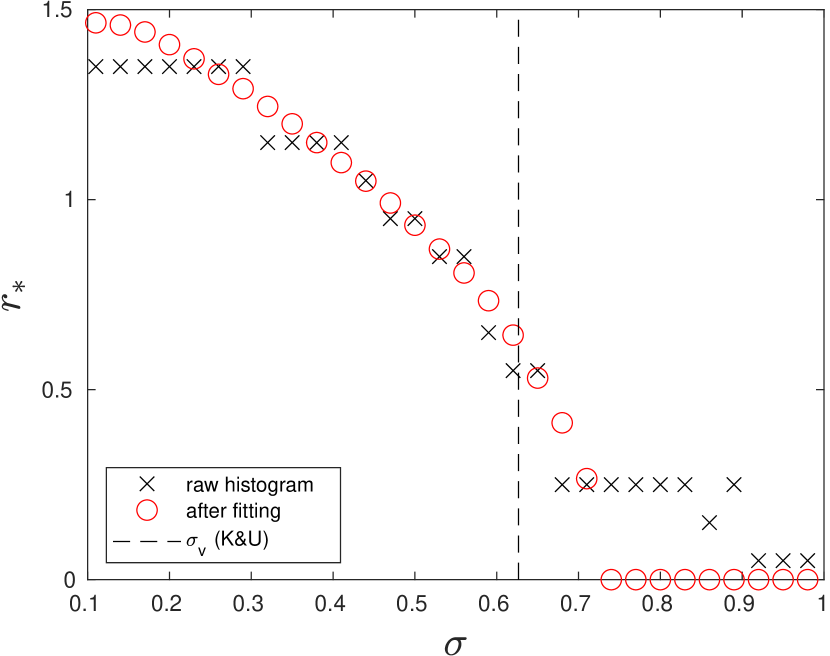
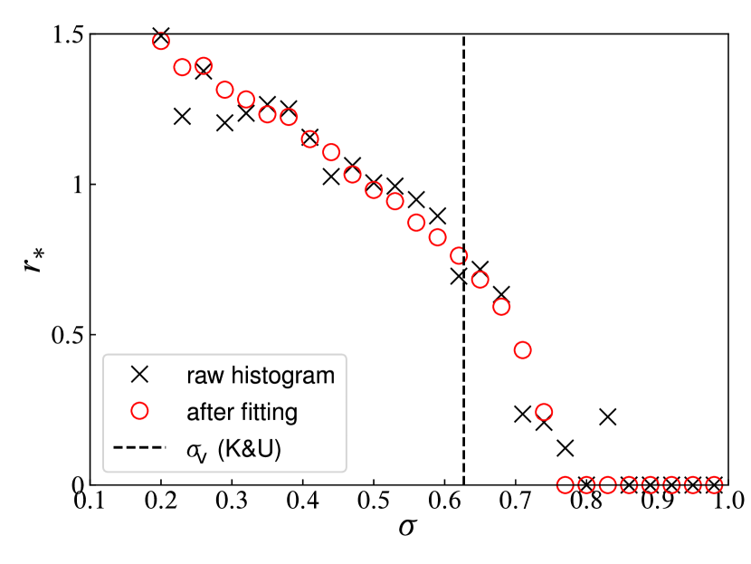
We have redone the simulation by Kimoto and Uezu (K&U) Kimoto and Uezu (2019), using the same population size $N=500$, and a coupling strength $\tilde{J}=1$. Following Kimoto and Uezu (2019) the frequency dispersion $\sigma$ was decreased quasiadiabatically, with a step size $\Delta\sigma=1.5\times 10^{-4}$, slightly smaller than $\Delta\sigma=\sqrt{\pi/2}\times 1.25\times 10^{-4}\simeq 1.567\times 10^{-4}$ used in Kimoto and Uezu (2019). The initial $\sigma$ value was 1.88, almost identical to $\sqrt{\pi/2}\times 1.5\simeq 1.87997$ used in Kimoto and Uezu (2019). Computation time for each $\sigma$ value was 800 t.u. long, while 10000 t.u. (recording the local fields every time unit) were run at specific $\sigma$ values, as in Kimoto and Uezu (2019).

The results for two completely independent numerical simulations are shown in Fig. 7. One data set (crosses) are the locations of the maximum of the histogram of local fields amplitudes, while the red circles are the values of $r_{*}$ after fitting the histogram to Eq. (27) in the main text. The prediction by K&U (coincident with our extrapolation from a low-rank coupling matrix) is

$$1=\frac{2}{\pi g(0)}=\sqrt{\frac{8}{\pi}}\sigma_{v}\qquad\Rightarrow\qquad\sigma_{v}=\sqrt{\frac{\pi}{8}}\simeq 0.627,$$ (28)

see dashed line in Fig. 7. In our view there is a nonnegligible discrepancy between theory and numerics. Alternatively, we can infer $\sigma_{v}$ from our numerical result in Fig. 5 with $N=400$. There we fixed $\sigma=\sqrt{\pi/2}$ and varied $\tilde{J}$. Now, we can move to $\sigma$ space obtaining

$$\sigma_{v}^{emp}=\frac{\sqrt{\pi/2}}{{\tilde{J}}_{v}^{emp}},$$ (29)

where ${{\tilde{J}}_{v}^{emp}}$ denotes the empirical critical coupling for the volcano transition in Fig. 5. According to Fig. 5 in the main text criticality is in the range $1.6<{\tilde{J}}_{v}^{emp}<1.7$, so we expect

$$0.737<\sigma_{v}^{emp}<0.783$$ (30)

This estimation is compatible with the results in Fig. 7. Nonetheless, an extensive study with more simulations, and ideally with larger systems sizes is probably in order.

Figure 7: Maximum of the distribution of local fields $r_{*}$ as a function of the frequency dispersion. Each panel corresponds to a completely independent numerical implementation (one by each author) using a 4th order Runge-Kutta algorithm of step size 0.1. Confront with Fig. 6(b) of Kimoto and Uezu (2019).

References

- Mézard et al. (1987) M. Mézard, G. Parisi, and M. A. Virasoro, Spin glass theory and beyond: An Introduction to the Replica Method and Its Applications, World Scientific Lecture Notes in Physics, Vol. 9 (World Scientific Publishing Company, Singapore, 1987).
- Daido (1992) H. Daido, “Quasientrainment and slow relaxation in a population of oscillators with random and frustrated interactions,” Phys. Rev. Lett. 68, 1073–1076 (1992).
- Sherrington and Kirkpatrick (1975) D. Sherrington and S. Kirkpatrick, “Solvable model of a spin-glass,” Phys. Rev. Lett. 35, 1792–1796 (1975).
- Stiller and Radons (1998) J. C. Stiller and G. Radons, “Dynamics of nonlinear oscillators with random interactions,” Phys. Rev. E 58, 1789–1799 (1998).
- Daido (2000) H. Daido, “Algebraic relaxation of an order parameter in randomly coupled limit-cycle oscillators,” Phys. Rev. E 61, 2145–2147 (2000).
- Stiller and Radons (2000) J. C. Stiller and G. Radons, “Self-averaging of an order parameter in randomly coupled limit-cycle oscillators,” Phys. Rev. E 61, 2148–2149 (2000).
- Acebrón et al. (2005) J. A. Acebrón, L. L. Bonilla, C. J. Pérez-Vicente, F. Ritort, and R. Spigler, “The Kuramoto model: A simple paradigm for synchronization phenomena,” Rev. Mod. Phys. 77, 137–185 (2005).
- Kimoto and Uezu (2019) T. Kimoto and T. Uezu, “Correspondence between phase oscillator network and classical XY model with the same random and frustrated interactions,” Phys. Rev. E 100, 022213 (2019).
- Bonilla et al. (1993) L.L. Bonilla, C.J. Pérez Vicente, and J.M. Rubí, “Glassy synchronization in a population of coupled oscillators,” J. Stat. Phys. 70, 921–937 (1993).
- Kloumann et al. (2014) I. M. Kloumann, I. M. Lizarraga, and S. H. Strogatz, “Phase diagram for the Kuramoto model with van Hemmen interactions,” Phys. Rev. E 89, 012904 (2014).
- Uezu et al. (2015) T. Uezu, T. Kimoto, S. Kiyokawa, and M. Okada, “Correspondence between phase oscillator network and classical XY model with the same infinite-range interaction in statics,” J. Phys. Soc. Jpn. 84, 033001 (2015).
- Ottino-Löffler and Strogatz (2018) B. Ottino-Löffler and S. H. Strogatz, “Volcano transition in a solvable model of frustrated oscillators,” Phys. Rev. Lett. 120, 264102 (2018).
- Fruchart et al. (2021) M. Fruchart, R. Hanai, P. B. Littlewood, and V. Vitelli, “Non-reciprocal phase transitions,” Nature 592, 363–369 (2021).
- Montbrió and Pazó (2018) E. Montbrió and D. Pazó, “Kuramoto model for excitation-inhibition-based oscillations,” Phys. Rev. Lett. 120, 244101 (2018).
- Laing et al. (2021) C. R. Laing, C. Bläsche, and S. Means, “Dynamics of structured networks of Winfree oscillators,” Front. Syst. Neurosci. 15, 631377 (2021).
- Hong and Strogatz (2011) H. Hong and S. H. Strogatz, “Kuramoto model of coupled oscillators with positive and negative coupling parameters: An example of conformist and contrarian oscillators,” Phys. Rev. Lett. 106, 054102 (2011).
- Uchida and Golestanian (2010) N. Uchida and R. Golestanian, “Synchronization in a carpet of hydrodynamically coupled rotors with random intrinsic frequency,” Europhys. Lett. 89, 50011 (2010).
- Hanai (2022) R. Hanai, “Non-reciprocal frustration: time crystalline order-by-disorder phenomenon and a spin-glass-like state,” arXiv preprint arXiv:2208.08577v2 (2022).
- Martí et al. (2018) D. Martí, N. Brunel, and S. Ostojic, “Correlations between synapses in pairs of neurons slow down dynamics in randomly connected neural networks,” Phys. Rev. E 97, 062314 (2018).
- Berlemont and Mongillo (2022) K. Berlemont and G. Mongillo, “Glassy phase in dynamically-balanced neuronal networks,” bioRxiv (2022), 10.1101/2022.03.14.484348.
- Note (1) In that case since .
- Ott and Antonsen (2008) E. Ott and T. M. Antonsen, “Low dimensional behavior of large systems of globally coupled oscillators,” Chaos 18, 037113 (2008).
- Note (2) For completeness: The imaginary eigenvalues of are . A sketch of the proof follows. We denote the normalized eigenvectors of with positive (negative) eigenvalue by () . From the identities , we find that and . The eigenvectors of are of the form , and the associated eigenvalues are , completing in this way the proof.
- Note (3) See the Supplemental Material at […] for details.
- Mastrogiuseppe and Ostojic (2018) F. Mastrogiuseppe and S. Ostojic, “Linking connectivity, dynamics, and computations in low-rank recurrent neural networks,” Neuron 99, 609–623 (2018).
- Schuessler et al. (2020) F. Schuessler, A. Dubreuil, F. Mastrogiuseppe, S. Ostojic, and O. Barak, “Dynamics of random recurrent networks with correlated low-rank structure,” Phys. Rev. Res. 2, 013111 (2020).
Supplemental Material to