Complexity of fermionic states

Abstract

How much information a fermionic state contains? To address this fundamental question, we define the complexity of a particle-conserving many-fermion state as the entropy of its Fock space probability distribution, minimized over all Fock representations. The complexity characterizes the minimum computational and physical resources required to represent the state and store the information obtained from it by measurements. Alternatively, the complexity can be regarded a Fock space entanglement measure describing the intrinsic many-particle entanglement in the state. We establish universal lower bound for the complexity in terms of the single-particle correlation matrix eigenvalues and formulate a finite-size complexity scaling hypothesis. Remarkably, numerical studies on interacting lattice models suggest a general model-independent complexity hierarchy: ground states are exponentially less complex than average excited states which, in turn, are exponentially less complex than generic states in the Fock space. Our work has fundamental implications on how much information is encoded in fermionic states.

I Introduction

The complexity of an object or a process quantifies how something can be generated from simple building blocks in an optimal way. For example, the computational complexity of a mathematical operation is defined in terms of the number of elementary operations required in its execution, or the complexity of a unitary operation in a quantum computer is defined as a the minimum number of elementary quantum gate operations required in its generation.Nielsen et al. (2006); Nielsen and Chuang (2010) Various notions of complexity in quantum systems and their relation to quantum information processing has been actively studied recently.Susskind (2016); Chapman et al. (2018); Balasubramanian et al. (2022) In this work, we introduce the complexity of $N$-particle fermionic states. The complexity quantifies how resource intensive it is to express a given state as a linear combination of Slater states (fermionic product states), which are the building blocks of the fermionic Fock space. If the complexity of a state is $\mathcal{C}$, to express this state in any Fock basis, one needs to specify at least $\mathcal{C}$ nonzero coefficients. We show that the complexity provides a bound for how much the information in the state can be compressed, thus determining the minimal physical and computational resources required to represent the state. Sophisticated numerical methodsSchollwöck (2005); Orús (2019) have been developed to mitigate the exponential complexity of correlated systems, however, only a genuine quantum simulationFeynman (1982) can be expected to incorporate it in general. Our results provide quantitative estimate for the complexity of distinct classes of states, outlining required resources for the quantum simulation targeting fermionic states.González-Cuadra et al. (2023); Bravyi and Kitaev (2002); Abrams and Lloyd (1997); Ortiz et al. (2001)

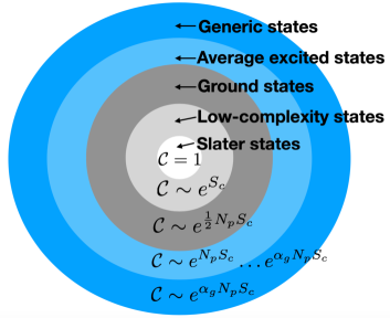
Figure 1: Complexity hierarchy of fermionic states as a function of particles $N_{p}$ and the correlation entropy $S_{c}$ at fixed filling fraction. Ground states and excited states refer to eigenstates of interacting lattice Hamiltonians at strong coupling exceeding the bandwidth and $1\leq\alpha_{g}\leq 2$, depending on the filling.

Besides its computational and information-theoretic implications, the complexity constitutes an entanglement measure in the Fock space. In contrast to widely studied partition entanglement measures,Amico et al. (2008) the complexity describes intrinsic partition-independent properties of $N$-particle states. It sharply distinguishes between the states of interacting and noninteracting Hamiltonians: all non-degenerate eigenstates of noninteracting systems can be represented as a single Slater state, thus having a trivial complexity.

The central finding in our work is that the complexity for distinct classes of states can be faithfully estimated from the correlation entropy $S_{c}$, defined essentially as the entanglement entropy between a single particle and the rest of the system. This quantity, exhibiting intensive size scaling, is calculated from the eigenvalues of the single-particle correlation matrix, and thus easily available in many numerical and theoretical methods. Specifically, i) we establish a universal lower bound for the complexity $S_{P}\geq S_{c}$, where $S_{P}$ is the logarithmic complexity $\mathcal{C}=e^{S_{P}}$ ii) we introduce a model-independent finite size complexity scaling hypothesis $S_{P}\sim\alpha N_{p}S_{c}$ for homogeneous $N_{p}$-particle states with constant filling fraction iii) numerical studies of interacting lattice models suggest that the coefficient $\alpha$ characterizes universal features of distinct classes of states, implying the exponential complexity hierarchy summarized in Fig. 1. In strongly coupled lattice models, the ground states are exponentially less complex than average excited states, which in turn are exponentially less complex than the generic states in the Fock space. Due to the model-independent nature of the scaling hypothesis, we postulate that the same complexity scaling is applicable for a broad class of local Hamiltonians. Our work has fundamental implications on how much information is contained in fermionic states.

II Fermionic complexity

We begin by defining the complexity for an arbitrary fermionic state $|\Phi\rangle$ in the Fock space of $N_{p}$ identical particles and $N_{o}$ available single-particle orbitals. This state can be expanded as

$$|\Phi\rangle=\sum_{k=1}^{k_{max}}a_{\{n_{B_{i}}\}_{k}}|\{n_{B_{i}}\}_{k}\rangle$$

where $B_{i}$ denotes orbital $i$ in the single-particle basis $\mathcal{B}$, and $\{n_{B_{i}}\}_{k}$ labels the distinct sets of single particle occupation numbers $n_{B_{i}}=0,1$. The $N_{p}$-particle Slater basis states are defined as $|\{n_{B_{i}}\}_{k}\rangle=\hat{c}^{\dagger}_{B_{jN_{p}}}\ldots\hat{c}^{\dagger}_{B_{j2}}\hat{c}^{\dagger}_{B_{j1}}\ket{0}$, where the product of fermion creation operators contains the populated orbitals in the set $\{n_{B_{i}}\}_{k}$. Each Slater state is multiplied with a nonzero complex probability amplitude $a_{\{n_{B_{i}}\}_{k}}\neq 0$. Depending on $|\Phi\rangle$ and the employed single-particle orbitals $\mathcal{B}$, the number of terms $k_{max}$ varies between 1 and the Fock space dimension $Q=\binom{N_{o}}{N_{p}}$. We now consider the 2nd Renyi entropy of the probability distribution of the Slater states

$$S_{P_{\mathcal{B}}}=-\ln{\sum_{k}P_{k}^{2}},$$

where $P_{k}=|a_{\{n_{B_{i}}\}_{k}}|^{2}$ denotes the probability weight of $|\{n_{B_{i}}\}_{k}\rangle$ in $|\Phi\rangle$. To eliminate the dependence on $\mathcal{B}$, we define the logarithmic complexity as

$$S_{P}=\min_{\mathcal{B}}S_{P_{\mathcal{B}}},$$ (1)

where the minimization is carried over all possible single-particle bases $\mathcal{B}$. Finally, we define the complexity of the state $|\Phi\rangle$ as

$$\mathcal{C}=e^{S_{P}}.$$

In practical calculations, carrying out the minimization in Eq. (1) is highly nontrivial task. Remarkably, as seen below, for the eigenstates of the studied lattice Hamiltonians, the optimal basis is excellently approximated by the correlation matrix eigenbasis and the position basis at weak and strong coupling.

The complexity, as defined above, has two illuminating interpretations: i) The complexity of a state determines its maximum compression in the Fock space, characterizing the number of terms in the most compact representation. In addition, by employing fundamental results in classical and quantum information theoryShannon (1948); Schumacher (1995); Preskill (2015), it can be shown that the maximum compression of the quantum information obtained by measurements is determined by the complexity. These aspects are discussed in Sec. A of Methods. Thus, complexity can be regarded as a basis-independent measure of $N$-particle information in a fermionic state, characterizing the minimum computational and physical resources to represent and store it. ii) The complexity of a state describes its intrinsic $N$-particle entanglement. Without entanglement, the state could be represented as a single Slater state. If the state has complexity $\mathcal{C}$, the amount of entanglement corresponds to that in an equal superposition of $\mathcal{C}$ Slater states. In contrast to the entanglement entropy and other partition-based measures, the complexity does not depend on arbitrary case-specific partition. Moreover, the complexity sharply distinguishes interacting and non-interacting systems since all non-degenerate eigenstates of quadratic Hamiltonians can be represented as a single Slater state with $S_{P}=0$, irrespective whether they obey the area-lawEisert et al. (2010), the volume-lawBianchi et al. (2022) or the critical entanglement entropy scaling.

II.1 Complexity lower bound from natural orbitals

A central role in the complexity is played by the single-particle correlation matrix, also known as the one-body reduced density matrix,

$$C_{ij}=\langle\Phi|\hat{c}^{\dagger}_{j}\hat{c}_{i}|\Phi\rangle,$$

where $\hat{c}^{\dagger}_{i},\hat{c}_{j}$ denote the fermionic creation and annihilation operators and indices $i,j\in 1\dots N_{o}$ label all possible single-particle orbitals in a fixed basis. If we have a system with $N_{o}$ available orbitals, the correlation matrix has dimension $N_{o}\times N_{o}$. Due to Fermi statistics, the correlation matrix eigenvalues satisfy $0\leq\lambda_{i}\leq 1$ and $\sum_{i}\lambda_{i}=N_{p}$. Thus, they can be interpreted as single-orbital occupation probabilities in the eigenbasis of $C_{ij}$. The eigestates of $C_{ij}$ are commonly referred as the natural orbitalsLöwdin (1955), which have found modern applications in analyzing strongly correlated many-body systems.Boguslawski et al. (2012); Aikebaier et al. (2023) We can define one-particle correlation entropy in the state $|\Phi\rangle$ as

$$S_{c}^{p}=-\ln{\frac{\sum_{i}\lambda_{i}^{2}}{N_{p}}},$$

which is a measure of how the occupation probabilities of the natural orbitals collectively differ from 1 or 0. As discussed in Sec. B in Methods, up to a trivial constant, $S_{c}^{p}$ is equal to the Renyi entanglement entropy between a single particle and the rest of the system, clarifying the role of $S_{P}$ as a novel entanglement measure. By interchanging the role of particles and holes, we define single-hole occupation probabilities $\tilde{\lambda}_{i}=1-\lambda_{i}$, which satisfy $0\leq\tilde{\lambda}_{i}\leq 1$ and $\sum_{i}\tilde{\lambda}_{i}=N_{o}-N_{p}$. We then define a single-hole correlation entropy as

$$S_{c}^{h}=-\ln{\frac{\sum_{i}\tilde{\lambda}_{i}^{2}}{N_{o}-N_{p}}},$$

and the correlation entropy as the larger of the two

$$S_{c}=\mathrm{max}\left\{S_{c}^{p},S_{c}^{h}\right\}.$$ (2)

In Sec. C in Methods we prove that, for arbitrary fermionic state $|\Phi\rangle$, the correlation entropy provides a lower bound for the logarithmic complexity

$$S_{P}\geq S_{c}.$$ (3)

This complexity bound is nontrivial: there exist states with nonzero logarithmic complexity for which the lower bound is saturated. A simple example is obtained by considering states where the number of particles $N_{p}$ and available orbitals $N_{o}$ satisfy $nN_{p}\leq N_{o}$ with $n\geq 2$. Given a single-orbital basis, one can find at least $n$ disjoint occupation number sets $\{n_{B_{i}}\}_{k}$ where each occupied orbital with $n_{B_{i}}=1$ belongs precisely to one set. Forming a superposition of such occupation sets $|\psi\rangle=\sum_{k=1}^{n}\sqrt{P_{k}}|\{n_{B_{i}}\}_{k}\rangle$, with $\sum_{k}P_{k}=1$, yields an example of a complexity bound saturating state. For these states the correlation matrix $C$ is diagonal, and the natural occupations $\lambda_{i}=C_{ii}=P_{k}$ for each of the $N_{p}$ occupied orbitals in the set $\{n_{B_{i}}\}_{k}$. Thus, $S_{c}=S_{p}=-\ln\sum_{i}^{n}P_{i}^{2}$, and the lower bound in (3) is saturated. The state $|\psi\rangle$ can also be regarded as an $n$-orbital generalization of the Greenberger-Horne-Zeilinger state $\frac{1}{\sqrt{2}}\left(|\uparrow\uparrow\uparrow\ldots\rangle+|\downarrow\downarrow\downarrow\ldots\rangle\right)$.Migdał et al. (2013) These type of states, whose complexity do not scale with the total number of particles at fixed filling fraction $\nu=\frac{N_{p}}{N_{o}}$, define the low-complexity category in Fig. 1. This category include, for example, eigenstates of impurity systems with a non-extensive number of scattering centers, such as the Kondo model. Despite a macroscopic reorganization of the Fermi sea, the eigenstates have only a few correlation matrix eigenvalues that differ from 0 or 1.Debertolis et al. (2021)

II.2 Complexity scaling

The existence of the lower-bound (3) saturating states suggests that the bound cannot be significantly improved without making additional assumptions of the states of interest. Eigenstates of local interacting Hamiltonians and other large-scale homogeneous states defined on a $d$-dimensional spatial lattice constitute a class of central importance. They define a family of states which can be studied as a function of the system size for a fixed filling fraction $\nu$. How is the complexity of such states scaling as the system size grows? For a generic filling fraction $\nu\neq 0,1$, the dimension of the Fock space of such states grows exponentially in $N_{p}$. Thus, in the leading order, we expect that the logarithmic complexity scales as $S_{P}\sim N_{p}$. However, the maximum value of the correlation entropy does not scale with the system size $S_{c}\leq\max\{-\ln\nu,-\ln(1-\nu)\}$. This shows that $S_{c}$ alone does not provide an accurate approximation for the complexity of these states. However, the role of $S_{c}$ in Eq. (3) suggests that it encodes some universal features of the complexity. Combining this idea with the exponential scaling in the system size, we postulate that the complexity of uniform states follows, in the leading order, the scaling form

$$S_{P}\sim\alpha N_{i}S_{c},$$ (4)

where $\alpha>0$ captures universal features of distinct classes of states. Here $N_{i}$ is the number of particles $N_{i}=N_{p}$ when $\nu\leq\frac{1}{2}$, and the number of holes $N_{i}=N_{o}-N_{p}$ when $\nu>\frac{1}{2}$. We illustrate this hypothesis for three paradigmatic examples: the Hubbard model of spinful fermions

$$\hat{H}=t\sum_{\langle i,j\rangle,\sigma}\left(\hat{c}^{\dagger}_{i\sigma}\hat{c}_{j\sigma}+\mathrm{h.c.}\right)+U\sum_{\langle i,j\rangle,\sigma}\hat{n}_{i\sigma}\hat{n}_{i\bar{\sigma}},$$

the $t-V$ model of spinless fermions

$$\hat{H}=\sum_{\langle i,j\rangle}\left(t\hat{c}^{\dagger}_{i}\hat{c}_{j}+\mathrm{h.c.}+V\hat{n}_{i}\hat{n}_{j}\right),$$

and Haar-distributed states, which we call “generic states” as they represent uniformly distributed unit vectors in the Fock space (see Sec. D in Methods). We observe that, indeed, the value of $\alpha$ distinguishes different broad classes of states:

1. The generic states have $\alpha=\alpha_{g}$, where $1\leq\alpha_{g}\leq 2$, depending on the filling fraction. The maximum $\alpha_{g}=2$ is obtained at $\nu=\frac{1}{2}$, while $\alpha_{g}\to 1$ when $\nu\to 0$ or $\nu\to 1$.

2. For non-degenerate ground states, $\alpha=\frac{1}{2}$ provides an excellent lower bound, which can become tight in various limits.

3. Average excited states have $1\lesssim\alpha<\alpha_{g}$ when the interaction exceeds the bandwith.

The difference in $\alpha$, despite its innocent appearance, translates into an exponential difference in the complexity.

Figure 2: Complexity of ground states. a): Ground state complexity of a half-filled Hubbard chain as a function of interaction. The system length is $L=8$ sites ($N_{o}=16$ orbitals). The numerically optimized complexity (black dots) is well-approximated from below by the ground state scaling form $S_{P}=\frac{1}{2}N_{p}S_{c}$ (green dashed line). The solid lines correspond to complexities calculated in the momentum and position orbitals. Complexity at weak coupling does not approach zero due to ground state degeneracy in the non-interacting model. b): Complexity scaling of the half filled Hubbard chain as a function of the particle number $N_{p}$. The complexity $S_{P}$ is approximated by $S_{min}=\min(S_{pos},S_{mom})$, as we cannot perform the full optimization for large systems. c): Tentative extrapolation of the coefficient $\alpha=S_{P}/(N_{p}S_{c})$ to infinite system size. The dashed lines are a quadratic fit. At strong coupling the value approaches $\alpha\approx 1/2$. d)-f): The same quantities for the $t-V$ model but at $\nu=1/3$ filling. Here we also explicitly include the complexity $S_{nat}$ in natural orbitals, which always gives the approximated minimal complexity $S_{min}$. Again, the ground state complexity follows closely the scaling form $S_{P}=\frac{1}{2}N_{p}S_{c}$.

The complexity of generic states provides a baseline reference to compare other types of states. The analytical expression for $\alpha_{g}$ is derived in the Sec. D in Methods. The generic states saturate the maximum value of the correlation entropy $S_{c}$ and the maximal leading order complexity allowed by the dimensionality of the Fock space. As seen below, the eigenstates of local Hamiltonians allow exponential compression compared to the generic states.

In Fig. 2 we illustrate the ground state complexity for the Hubbard model for $\nu=\frac{1}{2}$ and the $t-V$ for $\nu=\frac{1}{3}$. The minimizing basis, found by the conjugate gradient optimization (see Sec. D in Methods for details), is well approximated by the momentum states at weak coupling. In this case, the momentum basis is a natural orbital basis, however, the natural orbitals are not unique due to degeneracies in the natural occupations. For the $t-V$ model, the natural orbitals are essentially the optimal basis also at strong coupling, while for the Hubbard chain, the optimal basis at strong coupling coincides with the position orbitals. The ground state complexity for both models is seen to satisfy $S_{P}\gtrsim\frac{1}{2}N_{p}S_{c}$, where the lower bound appears tight for small $V$ and large $U$. In the Hubbard chain, the correlation entropy saturates the maximum value $S_{c}=\ln 2$ at strong coupling. Thus the logarithmic complexity of a generic state at half filling, $S_{P}=2N_{p}\ln 2$, is four times larger than that of the ground state of the Hubbard chain $S_{P}\approx\frac{1}{2}N_{p}\ln 2$ at strong coupling. Furthermore, the size scaling suggests that $\alpha$ converges reasonably close to $\alpha=\frac{1}{2}$ for all coupling strengths. This is observed for both models at fillings for which the ground state is non-degenerate. For the $t-V$ model at half filling, the ground state corresponds to two near-degenerate charge density wave configurations. In this case, we observe that the complexity of each charge-density wave state is well-captured by $S_{P}\sim\frac{1}{2}N_{p}S_{c}$.

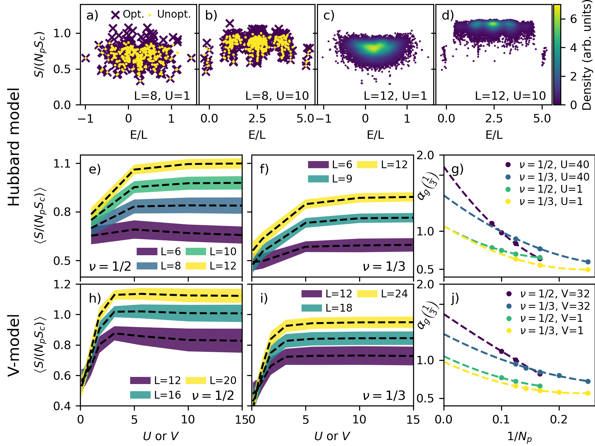
Figure 3: Complexity of excited states in the Hubbard and the $t-V$ model in the ground state parity and momentum sector. a)-b): Comparison of numerically optimized results $S_{opt}$ with $S_{min}=\min(S_{nat},S_{mom},S_{pos})$, where $S_{nat}$, $S_{mom}$ and $S_{pos}$ are the natural orbital, momentum and position basis complexities in a Hubbard chain of length $L=8$. c)-d): Distribution of the excited state complexity ratio $S/(N_{p}S_{c})$ for a larger system of $L=12$. e)-f): Mean complexity ratio in the ground state sector of the Hubbard model for filling factors $\nu=1/2$ and $\nu=1/3$. The colored areas around the mean (dashed line) have a width of one standard deviation. g): Scaling of the mean complexity with the number of particles $N_{p}$. For comparison, generic states have $\alpha_{g}=2$ at $\nu=1/2$ and $\alpha_{g}$ at $\nu=1/3$ is marked on the axis. h)-j): the same as e)-f) but for the $t,V$ model instead of the Hubbard model.

In Fig. 3 we analyze the complexity of excited states, for the same systems as in Fig. 2, by performing a full diagonalization in the parity and center-of-mass momentum sector which contains the ground state. For the excited states, finding numerically the minimizing basis becomes more challenging. As seen in Figs.3 a)-b), the numerical optimization does not find the true minimum for some high-complexity states. However, in the vast majority of cases, the optimization converges very close to the minimum value over natural, momentum and position orbitals. This indicates that, like for the ground states, one obtains an accurate approximation for the complexity by analyzing only these orbitals, especially when considering averages over many states. For both models, the average complexity of the excited states grows as a function of interaction and saturates to a constant at $U/t,V/t\approx 4$. At strong coupling, the average complexity is substantially higher than for the ground states. While the full diagonalization is restricted to modest system sizes, a fact one should be conscious of in extrapolating the results, Fig. 3 g) and f) imply that the ratio $S_{P}/(N_{p}S_{c})$ for the average excited states converge to a constant $\alpha<\alpha_{g}$. The specific value of $\alpha$ depends on the coupling strength and filling, but the average excited states remain, even around the midspectrum, significantly less complex than generic states. This behaviour is markedly different from the entanglement entropy, which exhibits identical leading order volume-law scaling for the midspectrum states of nonintegrable Hamiltonians and generic states. Vidmar and Rigol (2017); Bianchi et al. (2022); Kliczkowski et al. (2023)

III Discussion

In the above, we have seen how the complexity hierarchy summarized in Fig. 1 emerges. The single-Slater states, such as the eigenstates of quadratic Hamiltonians, have trivial complexity and are regarded as the fundamental building blocks of more complex states. For the low-complexity states, for which the complexity is not scaling with the system size when filling fraction is fixed, the complexity can be estimated from the universal lower bound $S_{c}$. As seen above, the ground state complexity is typically well captured by the scaling Ansatz (4) with prefactor $\alpha=1/2$. When the interaction exceeds the bandwidth, the complexity of average excited states follow (4) with $1\lesssim\alpha<\alpha_{g}$, where the upper bound determines the complexity of generic states. The model-independent nature of the scaling hypothesis and the qualitative agreement of different models suggest that the above results are not sensitive to the specific form of the Hamiltonian, as long as some broad features, such as locality and large scale homogeneity, are satisfied.

IV Conclusion and outlook

We introduced the complexity of a fermionic state to quantify the amount of information in it. The complexity provides a bound to the quantum state compression by choosing an optimal Fock basis, determining the minimum computational and physical resources to represent states. We showed that, for distinct classes of states, the complexity can be estimated from the eigenvalues of the single-particle correlation matrix. Considering the rapidly increasing interest in fermionic quantum simulation and quantum information processing, our results open several topical avenues of research. Does the observed complexity scaling laws for ground states and excited states represent a fundamental limit in encoding information to the eigenstates of local Hamiltonians? Do the complexity scaling laws, as their model-independent form suggests, also hold for higher dimensional systems? How can the scaling laws for eigenstates be derived from general arguments? How does the notion of Fock complexity, as studied here, reflect the circuit complexity of concrete fermionic quantum simulation schemes?González-Cuadra et al. (2023) To what extent the discovered complexity structure applies to bosonic states? Answers to these questions would provide fundamental new insight in many-body systems and their quantum information applications.

V Methods

V.1 Complexity as a fundamental bound to quantum state compression

Here we illustrate two aspects of the complexity: its role as a characteristic number of terms in the minimal Fock representation, and determining the minimal physical resources to store the quantum information extracted by measurements.

V.1.1 Complexity as the characteristic number of terms in the minimal Fock representation

The complexity of a state is connected to the characteristic number of terms which are required to span it in the optimal basis. Let $\{P_{n}\}$ be the probabilities in the optimal Fock basis which determines the complexity and let’s assume that the distribution is arranged in non-increasing order $P_{n_{1}}\geq P_{n_{2}}$ when $n_{1}<n_{2}$. How many terms are needed in the optimal basis to effectively span the state? Specifically, how large should $\tilde{n}$ be to satisfy $\sum_{n=1}^{\tilde{n}}P_{n}\sim 1$? This question is important for the states with large complexity $\tilde{n},\mathcal{C}\gg 1$ and the answer depends on the distribution: i) for sufficiently uniform distributions with a well-defined typical probability scale, the required number of terms is $\tilde{n}\sim\mathcal{C}$ ii) for heavy-tailed distributions, the required number of terms can scale nonlinearly in the complexity $\tilde{n}\sim\mathcal{C}^{\beta}$ with $\beta>1$.

Let’s first study i) and consider a case where the probabilities have a characteristic order of magnitude $P_{n}\sim P_{0}$ when $n\leq n^{\prime}$, and are strongly suppressed for $n>n^{\prime}$. This implies that $P_{0}\sim 1/n^{\prime}$ and $\mathcal{C}=1/\sum_{n}P^{2}\sim n^{\prime}$. Thus, the complexity roughly coincides with the effective cutoff index $n^{\prime}$ and we can conclude that $\sum_{n=1}^{\tilde{n}}P_{n}\sim 1$ is achieved when $\tilde{n}\sim\mathcal{C}$. When the distribution is strictly box distribution with constant probabilities $P_{0}=1/n^{\prime}$, the full probability is exactly recovered after $\mathcal{C}$ terms $\sum_{n=1}^{\mathcal{C}}P_{n}=1$. In general, to recover the full probability for distributions with a finite tail above $n=n^{\prime}$, one might need to include a few multiples of $\mathcal{C}$ terms. The linear scaling between $\tilde{n}$ and $\mathcal{C}$ reflects the typical expectation that entropy-like quantities scale as the logarithm of the total number of contributing states.

In case ii), the distribution has a long tail, the probabilities do not have a well-defined scale, and the previous reasoning breaks down. For this type of distributions, a nonlinear scaling $\tilde{n}\sim\mathcal{C}^{\beta}$ with a model-specific $\beta>1$ becomes possible. Such behaviour can be observed, for example, for power-law distributions and the distributions of eigenstates of lattice Hamiltonians, as illustrated in Fig. 4. For the ground state of a strongly coupled Hubbard model, we find that $\sum_{n=1}^{\mathcal{C}}P_{n}\sim 0.5$ and that the standard deviation and the complexity of the optimal distribution satisfy $\sigma=C^{\beta}$, where $\beta\lesssim 2$. Because most of the probability is located withing a few standard deviations, the full probability is covered by $\sum_{n=1}^{m\mathcal{C}^{\beta}}P_{n}\sim 1$, where $m$ is a small integer.

Figure 4: Cumulative probability distribution for the ground state of the Hubbard model at $U=10$, as a function of the scaled logarithm of the state index $\log(n)/L$. The state probabilities $P_{n}$ have been ordered from the largest to smallest. The vertical lines mark the scaled entropy $S_{P}/L$ and $\log(\sigma(n))/L$, where $\sigma(n)$ is the standard deviation of $n$. The inset shows a tentative extrapolation of $S_{P}/L$ and $\log(\sigma(n))/L$ to infinite system size.

To summarize, the complexity of a state provides a lower bound estimate for the characteristic number of terms in the optimal Fock representation.

V.1.2 Complexity and quantum information from measurements

In information theory, the notion of entropy was introduced to quantify the compression of strings of data which follows a known distribution.Shannon (1948) Analogously, the logarithmic complexity, which is an entropy quantity, characterizes the compression of the quantum information obtained by measurements. This can be made concrete by preparing $n$ copies of state $|\psi\rangle$ and performing repeated $N_{p}$-particle measurements in some Fock basis $|\{n_{B_{i}}\}_{k}\rangle$, where $\{n_{B_{i}}\}_{k}$ denotes an occupation number set in the single-orbital basis $\mathcal{B}$, and $k\in\{1,2,\ldots Q\}$ where $Q$ is the Fock space dimension. The resulting quantum states, obtained as outcomes of the $n$ measurements, constitutes the total information obtained from the measurements. This information can be stored as a composite state of the form

$$|\{n_{B_{i}}\}_{k_{1}}\rangle\otimes|\{n_{B_{i}}\}_{k_{2}}\rangle\otimes\ldots\otimes|\{n_{B_{i}},\}_{k_{n}}\rangle,$$ (5)

which is an element of $Q^{n}$-dimensional Hilbert space. However, in general, composite states of the form (5) do not fill this space densely. The complexity of $|\psi\rangle$ provides a fundamental lower bound of how much of the $Q^{n}$-dimensional space such states cover. In the language of quantum information theory, these composite states, obtained with probability $P_{k_{1}}^{\mathcal{B}}P_{k_{2}}^{\mathcal{B}}P_{k_{3}}^{\mathcal{B}}\ldots P_{k_{n}}^{\mathcal{B}}$, can be regarded as quantum messages constructed from individual letters, where each letter is a quantum state drawn from the ensemble $\left\{|\{n_{B_{i}}\}_{k}\rangle,P_{k}^{\mathcal{B}}\right\}$. Now one can ask how much these quantum messages can be compressed, or what is the minimum dimension of space $\mathcal{H}$ in which the messages can be accurately stored when $n$ is large. The dimension of $\mathcal{H}$ essentially determines the physical resources needed to store information extracted from $|\psi\rangle$. This formulation turns the problem into an application of Schumacher’s encoding theoremSchumacher (1995); Preskill (2015) in the special case where the letters form an orthogonal set. In this case, the quantum state of the messages is uniquely indexed by strings $k_{1}k_{2}\ldots k_{n}$. When $n$ is large, Shannon’s noiseless coding theorem implies that these strings can be faithfully compressed to $2^{nH(P_{k}^{\mathcal{B}})}$ long strings, where $H(P_{k}^{\mathcal{B}})=-\sum_{k}P_{k}^{\mathcal{B}}\log_{2}P_{k}^{\mathcal{B}}$ is the Shannon entropy.Shannon (1948); Preskill (2015) Thus, in this limit, almost all messages fit into a space of dimension $\log_{2}\left(\dim\mathcal{H}\right)=nH(P_{k}^{\mathcal{B}})$. The maximum compression is obtained in the Fock basis that minimizes $H(P_{k}^{\mathcal{B}})$. Since the Shannon entropy is bounded from below by the second Renyi entropy $H(P_{k}^{\mathcal{B}})\geq-\log_{2}\sum_{k}(P_{k}^{\mathcal{B}})^{2}$, the minimum $H(P_{k}^{\mathcal{B}})$ is bounded by the logarithmic complexity and

$$\ln(\dim\mathcal{H})\geq nS_{P}.$$ (6)

Thus, the complexity provides a lower bound to the dimension of $\mathcal{H}$, where the states obtained by $n$ measurements can be stored. Whenever the logarithmic complexity is smaller than its maximum value $\ln Q$, the composite states obtained from $|\psi\rangle$ by $n$ measurements do not fill the whole $Q^{n}$ dimensional space densely but only a subspace of it. This would allow compression of quantum information, with the maximum compression rate limited by the complexity. A dense filling would be obtained if $|\psi\rangle$ was a generic state for which the leading order logarithmic complexity is maximal.

V.2 Correlation entropy as an entanglement entropy

The single-particle correlation matrix in state $\left|\Phi\right\rangle$ is conventionally defined as $C_{ii^{\prime}}=\langle\Phi|\hat{c}^{\dagger}_{i^{\prime}}\hat{c}_{i}|\Phi\rangle$, which can also be written in first quantized notation as

$$C_{ii^{\prime}}=N_{p}\sum_{j,k,l,...}\Phi(i,j,k,l,...)\Phi(i^{\prime},j,k,l,...)^{*},$$

where $\Phi(i,j,k,l,...)$ is the antisymmetric wave function of the particles at coordinates $i,j,k,l,...$ .Löwdin (1955) Thus the actual normalized reduced density matrix of a single particle, defined as the partial trace over the coordinates of the other particles, is $\rho_{1}=C/N_{p}$,Ferreira et al. (2022) and the order $n$ Renyi entanglement entropy is defined as

$$S_{n}=\frac{1}{1-n}\ln(\mathrm{Tr}(\rho_{1}^{n})).$$

If $\left|\Phi\right\rangle$ is a single Slater determinant, $C$ has $N_{p}$ times degenerate eigenvalue $1$, the rest being zero. Therefore the entanglement entropies become

$$S^{\text{Slater}}_{n}=-\frac{1}{1-n}\log(N_{p}^{n-1}).~{}\text{(Slater state)}$$

However, in the spirit of the complexity $S_{P}$ which is trivial for Slater states, we subtract the free fermion contribution and define the single-particle correlation entropies as

$$S_{c,n}=S_{n}-S^{\text{Slater}}_{n}=\frac{1}{1-n}\ln\left(\mathrm{Tr}\left(\frac{C^{n}}{N_{p}}\right)\right).$$ (7)

$S_{c,2}$ is the particle correlation entropy discussed in the main text. Thus, the correlation entropy is actually a one-particle entanglement entropy from which the free fermion contribution has been subtracted.

V.3 Proof of the complexity lower bound

Here we will give a proof of the complexity lower bound (3) in three steps.

Proposition 1: Let’s consider a fermionic $N_{p}$ particle state $|\Phi\rangle$. Furthermore, let’s assume that $\lambda_{i}$ is the set of correlation matrix eigenvalues (occupation probabilities of the natural orbitals) and $\bar{n}_{B_{i}}$ are the occupation probabilities of single-particle orbitals in an arbitrary basis $\mathcal{B}$. They always satisfy $\sum_{i}\lambda_{i}^{2}\geq\sum_{i}{\bar{n}_{B_{i}}}^{2}$. Proof: Let $C$ be the correlation matrix. Then $\sum_{i}\lambda_{i}^{2}=\mathrm{Tr}\,C^{2}=\sum_{\alpha,\beta}C_{\alpha\beta}C_{\beta\alpha}=\sum_{\alpha,\beta}|C_{\alpha\beta}|^{2}\geq\sum_{\alpha}|C_{\alpha\alpha}|^{2}\equiv\sum_{\alpha}{\bar{n}_{B_{\alpha}}}^{2}$. Here we used the fact that the in the double sum all entries are positive and that occupation probabilities in a general basis are defined as diagonal entries of the correlation matrix.

Proposition 2: The average occupation numbers $\bar{n}_{B_{i}}$ and the state probabilities $P_{\{n_{B_{i}}\}_{k}}$ always satisfy $\sum_{i}\frac{\bar{n}_{B_{i}}^{2}}{N_{p}}\geq\sum_{k}P_{\{n_{B_{i}}\}_{k}}^{2}$. The first sum is over all the single-particle orbitals whereas the second sum is over all $k_{max}$ occupation number sets in Eq. (1). Proof: The average occupation numbers can be written in terms of the state probabilities as $\bar{n}_{B_{i}}=\sum_{k}P_{\{n_{B_{i}}\}_{k}}n_{B_{i}}^{k}$, where $n_{B_{i}}^{k}=0,1$ is the value of the occupation number of orbital $B_{i}$ in the set $\{n_{B_{i}}\}_{k}$. From this we get $\sum_{i}\bar{n}_{B_{i}}^{2}=\sum_{i}\sum_{k,l}P_{\{n_{B_{i}}\}_{k}}n_{B_{i}}^{k}P_{\{n_{B_{i}}\}_{l}}n_{B_{i}}^{l}\geq\sum_{i}\sum_{k}P_{\{n_{B_{i}}\}_{k}}^{2}n_{{B_{i}}_{k}}^{2}=\sum_{k}P_{\{n_{B_{i}}\}_{k}}^{2}\sum_{i}n_{{B_{i}}_{k}}^{2}=\sum_{k}P_{\{n_{B_{i}}\}_{k}}^{2}\sum_{i}n_{B_{i}}^{k}=\sum_{k}P_{\{n_{B_{i}}\}_{k}}^{2}N_{p}$. The inequality follows from dropping non-negative terms from the double sum. Comparing the starting and final form, we have proved Proposition 2.

Universal lower bound for $S_{P}$: using Property 1. and the monotonicity of logarithm, we deduce that $S_{c}^{p}=-\log{\frac{\sum_{i}\lambda_{i}^{2}}{N_{p}}}\leq-\log{\frac{\sum_{i}\bar{n}_{B_{i}}^{2}}{N_{p}}}$. Now, using Property 2 it follows that $S_{c}^{p}\leq-\log{\frac{\sum_{i}\bar{n}_{B_{i}}^{2}}{N_{p}}}\leq-\log{\sum_{k}P_{\{n_{B_{i}}\}_{k}}^{2}}=S_{P_{\mathcal{B}}}$. Since this holds for arbitrary basis $\mathcal{B}$, we can minimize the right-hand side over all bases and it still holds. Thus, we have proved that $S_{c}^{p}\leq S_{P}.$ The corresponding inequality for the hole correlation entropy $S_{c}^{h}\leq S_{P}$ can be straightforwardly established by exchanging the roles of particles and holes and tracing the same steps. Thus, we arrive at $S_{c}\leq S_{P}$ where $S_{c}$ is the larger one of $S_{c}^{p},S_{c}^{h}$.

V.4 Complexity of generic states

Figure 5: Complexity of generic, Haar-distributed states in different single-particle bases computed as a mean of five samples with the vertical bars giving the sample standard deviation, except at $N_{p}=6$ where we have only computed one realization. A Q-dimensional generic state has logarithmic complexity $S_{CUE}=-\log(2/Q)$ in the limit of large $Q$. The complexity can be reduced by applying single-particle rotations as demonstrated here by transforming to the natural orbital basis or a numerically optimized basis. However, to conserve information, we expect that the typical reduction in the characteristic number of terms $C=\exp(-S)$ in the optimal Fock representation of a state with no special structure scales with the number of parameters in the single-particle basis, i.e. polynomially in $N_{p}$, while $C$ grows exponentially for a fixed filling fraction. $S_{CUE,nat}$ and $S_{CUE,opt}$ are thus expected to approach $S_{CUE}$ for large $N_{p}$, while the correlation entropy approaches its maximal value $-\log(\nu)$.

Here we derive the complexity of generic states in a Fock space with $M$ available orbitals and $N_{p}$ particles with dimension $Q=\binom{N_{o}}{N_{p}}=\frac{N_{o}!}{(N_{o}-N_{p})!N_{p}!}$. Let’s start with some normalized vector in the Fock space $|\psi_{0}\rangle=\sum_{k=1}^{Q}a_{k}|k\rangle$, where $|k\rangle$ is some basis and $\sum_{k}|a_{k}|^{2}=1$ and consider all the states that can be obtained from $|\psi_{0}\rangle$ by unitary transformations:

$$|\psi\rangle=U|\psi_{0}\rangle=\sum_{k,j=1}^{Q}U_{jk}a_{k}|j\rangle.$$

These states fill the Fock space uniformly and are referred as generic states. To calculate the complexity, we extract the probabilities $P_{j}=|U_{jk}a_{k}|^{2}=U_{jk}U_{jl}^{*}a_{k}a_{l}^{*}$ (repeated indices are summed) and their squares $P_{j}^{2}=U_{jk}U_{jl}^{*}U_{jm}U_{jn}^{*}a_{k}a_{l}^{*}a_{m}a_{n}^{*}$. To evaluate the average $\langle P_{i}^{2}\rangle$ over the Haar measure, we can make use of the circular unitary ensemble resultForrester (2010)

$$\langle U_{jk}U_{jm}U_{jl}^{*}U_{jn}^{*}\rangle=\frac{1}{Q^{2}}\left(\delta_{kl}\delta_{mn}+\delta_{kn}\delta_{ml}\right)$$

for $Q\gg 1$. Employing the above formula, we obtain $\langle P_{j}^{2}\rangle=\frac{2}{Q^{2}}$, and

$$\sum_{j=1}^{Q}\langle P_{j}^{2}\rangle=\frac{2}{Q}$$

For large $Q\gg 1$, the average logarithmic complexity becomes $S_{P}=\langle-\ln{\sum_{i}P_{i}^{2}}\rangle=-\ln{\sum_{i}\langle P_{i}^{2}\rangle}=-\ln(2/Q)$. The expectation value can be moved inside the logarithm, because the argument becomes non-fluctuating in the large $Q$ limit. Also, the minimization over possible single-particle orbitals would not affect the result in large systems, since the number of optimization parameters scale linearly in orbitals while the independent components of the states vectors grow exponentially. The this behaviour is illustrated in Fig. 5, showing how the optimized complexity in small systems is approaching the above analytical results. By employing Stirling’s formula, the leading order complexity of generic states state becomes

$$S_{P}=-N_{o}\ln\left[\nu^{\nu}(1-\nu)^{1-\nu}\right],$$ (8)

where $\nu=N_{p}/N_{o}$. Since the generic states are uniformly distributed in space and cannot be compressed, their leading order complexity is the maximum allowed by the dimensionality of the Fock space. As illustrated in Fig. 5, the generic states also maximize the particle and hole correlation entropies $S_{c}^{p}=-\ln\nu$, $S_{c}^{h}=-\ln(1-\nu)$. Thus, the result (8) can be expressed in the general form (4) with $\alpha=\alpha_{g}$ where

$$\alpha_{g} =1+\frac{(1-\nu)\ln(1-\nu)}{\nu\ln(\nu)},\qquad 0\leq\nu\leq\frac{1}{2}$$

$$\alpha_{g} =1+\frac{\nu\ln(\nu)}{(1-\nu)\ln(1-\nu)},\qquad\frac{1}{2}<\nu\leq 1$$

V.5 Computational details

We perform exact diagonalization calculations using the QuSpin package Weinberg and Bukov (2017, 2019), which allows easy building of Hamiltonian matrices for the fermionic lattice models considered here. The package also allows selecting specific symmetry sectors of lattice models, fixing e.g. quantum numbers corresponding to center-of-mass momentum and parity under reflection $p\rightarrow-p$. For the excited state calculations we perform full diagonalization of the selected symmetry block using standard dense hermitian methods, while for the ground state results we employ ARPACK-based sparse methods included in the QuSpin library and Scipy Virtanen et al. (2020).

To study the entropy $S_{P_{\mathcal{B}}}$ in different bases $\mathcal{B}$, we need to change the single-orbital basis for the full many-body eigenstates which are initially computed in the position basis. In the second quantized formalism, an orbital transformation for a system with $N_{o}$ orbitals is specified by an $N_{o}\times N_{o}$ unitary matrix $U$ acting on the annihilation operators as

$$\vec{c^{\prime}}=U\vec{c},~{}\vec{c}=[c_{1},c_{2}\cdots,c_{N_{o}}]^{T}.$$ (9)

The unitary matrix can be parametrized by a hermitian matrix $A$ such that $U=\exp(iA)$, and this transformation can then be expressed as an operator $\hat{U}$ in the many-body Fock space as

$$\hat{U}=\exp(i\vec{c}^{\dagger}A\vec{c}),$$ (10)

acting on operators as $\hat{U}^{\dagger}\vec{c}\hat{U}=U\vec{c}$. That the orbital rotations can be expressed in such exponentiated form is referred to as the Thouless theorem Thouless (1960) in the literature Kivlichan et al. (2018).

The operator $\hat{A}=\vec{c}^{\dagger}A\vec{c}$ is represented as a sparse matrix that only couples basis states connected by a single hop, thus having $N_{p}N_{h}Q$ non-zero elements, where $N_{p}$ and $N_{h}$ are the number of particles and holes, respectively, and $Q$ is the number of Fock basis states. Applying the operator $\hat{U}$ on a state in the Fock space can be carried out by sparse matrix methods, where the only large matrix operation is matrix-vector multiplication by $\hat{A}$. Al-Mohy and Higham (2011); Higham and Al-Mohy (2010) For small systems, the non-zero matrix elements of $\hat{A}$ can be computed and stored in memory in a sparse matrix format. For large systems, it is advantageous to compute the matrix elements of $\hat{A}$ on the fly when performing the matrix-vector multiplication, as memory access becomes the bottleneck of the computation.

For basis optimization we again parametrize the orbital basis in the form $U=\exp(iA)$ and perform a conjugate gradient minimization of the Renyi entropy $S_{P_{\mathcal{B}}}$ with the elements of the hermitian matrix $A$ treated as free parameters. For the single-component models, we use a random matrix $U\sim\text{CUE}(N_{o})$ as the starting point of the minimization, with $N_{o}$ the number of orbitals in the model. For the two-component Hubbard model, we enforce component conservation meaning that $A$ is block-diagonal and does not mix different spin components.

VI Data availability

The data supporting the findings of this work are available upon reasonable request.

VII Code availability

The codes implementing the calculations in this work are available upon reasonable request.

VIII Author contributions

T.O. proposed the idea, which the authors developed together. T. I. V. developed the numerical approaches and carried out all numerical calculations. The manuscript was prepared jointly by the authors.

IX Acknowledgements

T.O. acknowledges the Academy of Finland (project 331094) and Jane and Aatos Erkko Foundation for support. Computing resources were provided by CSC – the Finnish IT Center for Science.

X Competing Interests

The authors declare no competing interests.

References

- Nielsen et al. (2006) Michael A. Nielsen, Mark R. Dowling, Mile Gu, and Andrew C. Doherty, “Quantum computation as geometry,” Science 311, 1133–1135 (2006), https://www.science.org/doi/pdf/10.1126/science.1121541 .
- Nielsen and Chuang (2010) Michael A. Nielsen and Isaac L. Chuang, Quantum Computation and Quantum Information: 10th Anniversary Edition (Cambridge University Press, 2010).
- Susskind (2016) Leonard Susskind, “Computational complexity and black hole horizons,” Fortschritte der Physik 64, 24–43 (2016), https://onlinelibrary.wiley.com/doi/pdf/10.1002/prop.201500092 .
- Chapman et al. (2018) Shira Chapman, Michal P. Heller, Hugo Marrochio, and Fernando Pastawski, “Toward a definition of complexity for quantum field theory states,” Phys. Rev. Lett. 120, 121602 (2018).
- Balasubramanian et al. (2022) Vijay Balasubramanian, Pawel Caputa, Javier M. Magan, and Qingyue Wu, “Quantum chaos and the complexity of spread of states,” Phys. Rev. D 106, 046007 (2022).
- Schollwöck (2005) U. Schollwöck, “The density-matrix renormalization group,” Rev. Mod. Phys. 77, 259–315 (2005).
- Orús (2019) Román Orús, “Tensor networks for complex quantum systems,” Nature Reviews Physics 1, 538–550 (2019).
- Feynman (1982) R. P. Feynman, “Simulating physics with computers,” Int. J. Theor. Phys. 21, 467 (1982).
- González-Cuadra et al. (2023) Daniel González-Cuadra, Dolev Bluvstein, Marcin Kalinowski, Raphael Kaubruegger, Nishad Maskara, Piero Naldesi, Torsten V. Zache, Adam M. Kaufman, Mikhail D. Lukin, Hannes Pichler, Benoît Vermersch, Jun Ye, and Peter Zoller, “Fermionic quantum processing with programmable neutral atom arrays,” (2023), arXiv:2303.06985 [quant-ph] .
- Bravyi and Kitaev (2002) Sergey B. Bravyi and Alexei Yu. Kitaev, “Fermionic quantum computation,” Annals of Physics 298, 210–226 (2002).
- Abrams and Lloyd (1997) Daniel S. Abrams and Seth Lloyd, “Simulation of many-body fermi systems on a universal quantum computer,” Phys. Rev. Lett. 79, 2586–2589 (1997).
- Ortiz et al. (2001) G. Ortiz, J. E. Gubernatis, E. Knill, and R. Laflamme, “Quantum algorithms for fermionic simulations,” Phys. Rev. A 64, 022319 (2001).
- Amico et al. (2008) Luigi Amico, Rosario Fazio, Andreas Osterloh, and Vlatko Vedral, “Entanglement in many-body systems,” Rev. Mod. Phys. 80, 517–576 (2008).
- Shannon (1948) C. E. Shannon, “A mathematical theory of communication,” Bell System Technical Journal 27, 379–423 (1948).
- Schumacher (1995) Benjamin Schumacher, “Quantum coding,” Phys. Rev. A 51, 2738–2747 (1995).
- Preskill (2015) J. Preskill, Lecture Notes for Physics 229:Quantum Information and Computation (CreateSpace Independent Publishing Platform, 2015).
- Eisert et al. (2010) J. Eisert, M. Cramer, and M. B. Plenio, “Colloquium: Area laws for the entanglement entropy,” Rev. Mod. Phys. 82, 277–306 (2010).
- Bianchi et al. (2022) Eugenio Bianchi, Lucas Hackl, Mario Kieburg, Marcos Rigol, and Lev Vidmar, “Volume-law entanglement entropy of typical pure quantum states,” PRX Quantum 3, 030201 (2022).
- Löwdin (1955) Per-Olov Löwdin, “Quantum theory of many-particle systems. i. physical interpretations by means of density matrices, natural spin-orbitals, and convergence problems in the method of configurational interaction,” Phys. Rev. 97, 1474–1489 (1955).
- Boguslawski et al. (2012) Katharina Boguslawski, Paweł Tecmer, Örs Legeza, and Markus Reiher, “Entanglement measures for single- and multireference correlation effects,” The Journal of Physical Chemistry Letters 3, 3129–3135 (2012).
- Aikebaier et al. (2023) Faluke Aikebaier, Teemu Ojanen, and Jose L. Lado, “Extracting electronic many-body correlations from local measurements with artificial neural networks,” SciPost Phys. Core 6, 030 (2023).
- Migdał et al. (2013) Piotr Migdał, Javier Rodriguez-Laguna, and Maciej Lewenstein, “Entanglement classes of permutation-symmetric qudit states: Symmetric operations suffice,” Phys. Rev. A 88, 012335 (2013).
- Debertolis et al. (2021) Maxime Debertolis, Serge Florens, and Izak Snyman, “Few-body nature of kondo correlated ground states,” Phys. Rev. B 103, 235166 (2021).
- Vidmar and Rigol (2017) Lev Vidmar and Marcos Rigol, “Entanglement entropy of eigenstates of quantum chaotic hamiltonians,” Phys. Rev. Lett. 119, 220603 (2017).
- Kliczkowski et al. (2023) M. Kliczkowski, R. Świętek, L. Vidmar, and M. Rigol, “Average entanglement entropy of midspectrum eigenstates of quantum-chaotic interacting hamiltonians,” (2023), arXiv:2303.13577 [cond-mat.stat-mech] .
- Ferreira et al. (2022) Diego L. B. Ferreira, Thiago O. Maciel, Reinaldo O. Vianna, and Fernando Iemini, “Quantum correlations, entanglement spectrum, and coherence of the two-particle reduced density matrix in the extended hubbard model,” Phys. Rev. B 105, 115145 (2022).
- Forrester (2010) Peter J. Forrester, Log-Gases and Random Matrices (Princeton University Press, 2010).
- Weinberg and Bukov (2017) Phillip Weinberg and Marin Bukov, “QuSpin: a Python package for dynamics and exact diagonalisation of quantum many body systems part I: spin chains,” SciPost Phys. 2, 003 (2017).
- Weinberg and Bukov (2019) Phillip Weinberg and Marin Bukov, “QuSpin: a Python package for dynamics and exact diagonalisation of quantum many body systems. Part II: bosons, fermions and higher spins,” SciPost Phys. 7, 020 (2019).
- Virtanen et al. (2020) Pauli Virtanen, Ralf Gommers, Travis E. Oliphant, Matt Haberland, Tyler Reddy, David Cournapeau, Evgeni Burovski, Pearu Peterson, Warren Weckesser, Jonathan Bright, Stéfan J. van der Walt, Matthew Brett, Joshua Wilson, K. Jarrod Millman, Nikolay Mayorov, Andrew R. J. Nelson, Eric Jones, Robert Kern, Eric Larson, C J Carey, İlhan Polat, Yu Feng, Eric W. Moore, Jake VanderPlas, Denis Laxalde, Josef Perktold, Robert Cimrman, Ian Henriksen, E. A. Quintero, Charles R. Harris, Anne M. Archibald, Antônio H. Ribeiro, Fabian Pedregosa, Paul van Mulbregt, and SciPy 1.0 Contributors, “SciPy 1.0: Fundamental Algorithms for Scientific Computing in Python,” Nature Methods 17, 261–272 (2020).
- Thouless (1960) D.J. Thouless, “Stability conditions and nuclear rotations in the hartree-fock theory,” Nuclear Physics 21, 225–232 (1960).
- Kivlichan et al. (2018) Ian D. Kivlichan, Jarrod McClean, Nathan Wiebe, Craig Gidney, Alán Aspuru-Guzik, Garnet Kin-Lic Chan, and Ryan Babbush, “Quantum simulation of electronic structure with linear depth and connectivity,” Phys. Rev. Lett. 120, 110501 (2018).
- Al-Mohy and Higham (2011) Awad H Al-Mohy and Nicholas J Higham, “Computing the action of the matrix exponential, with an application to exponential integrators,” SIAM journal on scientific computing 33, 488–511 (2011).
- Higham and Al-Mohy (2010) Nicholas J Higham and Awad H Al-Mohy, “Computing matrix functions,” Acta Numerica 19, 159–208 (2010).