A Half de Sitter Holography

Abstract

A long-standing and intriguing question is: does the holographic principle apply to cosmologies like de Sitter spacetime? In this work, we consider a half dS spacetime wherein a timelike boundary encloses the bulk spacetime, presenting a version of de Sitter holography. By analyzing the holographic entanglement entropy in this space and comparing it with that in AdS/CFT, we argue that gravity on a half dS_d+1 is dual to a highly non-local field theory residing on dS_d boundary. This non-locality induces a breach in the subadditivity of holographic entanglement entropy. Remarkably, this observation can be linked to another argument that time slices in global de Sitter space overestimate the degrees of freedom by redundantly counting the same Hilbert space multiple times.

1 Introduction

The holographic duality has bestowed upon us a promising framework, enabling the exploration of quantum gravity tHooft:1993dmi ; Susskind:1994vu . The most outstanding example will be the AdS/CFT correspondence where quantum gravity on $d+1$-dimensional Anti-de Sitter space (AdS_d+1) becomes equivalent to $d$-dimensional conformal field theory (CFT_d) Maldacena:1997re ; Gubser:1998bc ; Witten:1998qj . Despite the resounding success attained in AdS/CFT, we are still at a nascent stage in the development of the holographic duality pertaining to gravity in de Sitter space. The potential dS holography promises paramount application to realistic cosmological spacetime.

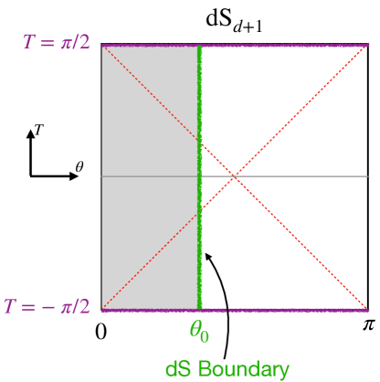
Figure 1: The Penrose diagram of dS_d+1 bulk spacetime. The conformal time $T\in[-\frac{\pi}{2},+\frac{\pi}{2}]$ is associated with the global time $t$ by $\cosh t=\frac{1}{\cos T}$. We introduce a timelike boundary at $\theta=\theta_{0}$ which is described by a $d-$dimensional dS spacetime. The dual bulk dS_d+1 spacetime is given by the gray shaded region.

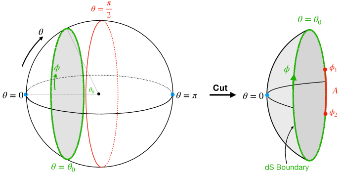
Figure 2: The left panel shows the geometry of time slices for a global dS₃. In the right panel we keep a half of dS₃ space with a dS₂ boundary (denoted by green circle) at $\theta=\theta_{0}$.

Let us commence by exploring the explicit differences between dS holography and AdS/CFT. The $d+1$-dimensional de Sitter space (dS_d+1) can be described in global coordinates as follows (see e.g., Spradlin:2001pw ; Galante:2023uyf for comprehensive reviews):

$$ds^{2}=-dt^{2}+\cosh^{2}td\Omega_{d}^{2},.$$ (1.1)

whose Penrose diagram is shown in figure 1. Here, we have set the dS radius to unity, and $d\Omega_{d}^{2}$ represents the metric of the unit $d$-dimensional sphere:

$$d\Omega_{d}=d\theta^{2}+\sin^{2}\theta d\Omega_{d-1}^{2}\,,$$ (1.2)

The constant time slice in global dS_d+1 coordinate is depicted in the left diagram of figure 3. In the case of $d=2$, we simply write $d\Omega_{d-1}^{2}=d\phi^{2}$ in this paper. As shown in the left panel of figure 1, the conformal boundaries of global dS spacetime are spacelike surfaces i.e., $S^{d}$, located at the future and past infinity $t=\pm\infty$. The original dS/CFT correspondence postulates that the gravitational dynamics in the dS_d+1 bulk is dual to a Euclidean conformal field theory (CFT) on the sphere S^d at future infinity $t\to\infty$ Spradlin:2001pw ; Witten:2001kn ; Maldacena:2002vr . This proposal assumes that the quantum state is generated by the Euclidean instanton using the Hartle-Hawking prescription and is then continued to Lorentzian dS at $t=0$. However, the dual CFT becomes non-unitary and exhibits numerous exotic characteristics. For instance, in the case of dS${}_{4}/$CFT₃, the 3D CFT dual to higher-spin gravity on dS₄ is described by the $SP(N)$ model, which incorporates ghost fields Anninos:2011ui ; Ng:2012xp . Similarly, for dS${}_{3}/$CFT₂, the 2D CFT dual to Einstein gravity on dS₃ is obtained through an analytical continuation of current algebra or Liouville CFT, with an imaginary central charge Hikida:2021ese ; Hikida:2022ltr ; Chen:2022ozy ; Chen:2023prz . Furthermore, holography for dS₂ has been investigated in Maldacena:2019cbz ; Cotler:2019nbi ; Cotler:2023eza . Despite the peculiar holographic properties, studies from the perspective of gravity have also been developed, with a partial list of references including Castro:2011xb ; Castro:2012gc ; Anninos:2020hfj ; Anninos:2021ihe ; Castro:2023dxp .

One of the manifestations of the non-unitary nature inherent in the dS/CFT correspondence is the computation of holographic entanglement entropy. In the context of the AdS/CFT correspondence, the holographic entanglement entropy $S_{A}$ for a subsystem $A$ in the dual CFT can be determined by evaluating the area of the extremal surface $\Gamma_{A}$ in AdS, which ends on the the boundary of the subsystem $A$ Ryu:2006bv ; Ryu:2006ef ; Hubeny:2007xt :

$$S_{A}=\frac{A(\Gamma_{A})}{4G_{\textrm{\tiny N}}}\,,$$ (1.3)

where $G_{\textrm{\tiny N}}$ denotes the Newton constant and $A(\Gamma_{A})$ represents the area of the extremal surface $\Gamma_{A}$. In principle, this geometric computation can be extended to various spacetimes, including de Sitter space. However, in de Sitter space, the absence of a spacelike extremal surface connecting two distinct points on S^d at future infinity leads to the holographic entanglement entropy being complex-valued Narayan:2015vda ; Sato:2015tta ; Hikida:2022ltr . In this context, the holographic entanglement entropy is computed by using the timelike extremal surface in de Sitter space. Subsequently, in Doi:2022iyj ; Doi:2023zaf , this complex-valued entropy was appropriately interpreted as the pseudo-entropy Nakata:2021ubr ; Mollabashi:2020yie ; Mollabashi:2021xsd , which generalizes the notion of entanglement entropy to non-Hermitian density matrices (see Narayan:2022afv ; Narayan:2023ebn for closely related ideas). This consideration suggests a connection between the emergent time coordinate in dS/CFT and the imaginary part of the pseudo-entropy. Notably, an intriguing quantum entanglement structure of dS holography has been recently proposed in Cotler:2023xku .

Several other approaches to de Sitter holography have been explored. One notable example is the holography for de Sitter space in the static patch, which has recently garnered significant attention and discussions from multiple perspectives Susskind:2021omt ; Susskind:2021esx ; Shaghoulian:2022fop ; Chapman:2021eyy ; Jorstad:2022mls ; Chandrasekaran:2022cip ; Anegawa:2023wrk ; Franken:2023pni . Additionally, another approach to dS holography has been investigated, based on the TTbar deformation in AdS/CFT McGough:2016lol and the dS/dS duality Alishahiha:2004md , with studies conducted in Dong:2018cuv ; Gorbenko:2018oov . An interesting dS/dS duality setup can also be found in Geng:2021wcq . The quantum information structure in de Sitter has been analyzed by applying the surface/state duality Miyaji:2015yva . Notably, it has been observed that the state dual to the $t=0$ slice is maximally entangled.

In this paper, we propose a novel approach to dS holography that adheres to the standard holographic formalism, wherein gravity in a given bulk space is dual to a non-gravitational theory on its timelike boundary. However, since de Sitter space lacks timelike boundaries, we introduce a procedure to create one. Our proposal involves cutting a de Sitter space into a half at $\theta=\theta_{0}$ by confining the sphere $S^{d}$ to a semi-sphere. More generally, we can cut the bulk dS space by putting a boundary at $\theta=\theta_{0}$, as depicted in figure 1 and 2. This resulting spacetime is referred to as a half de Sitter space (or simply half dS). The boundary of the $d+1$-dimensional half de Sitter space corresponds to $d$-dimensional global de Sitter spacetime dS_d, which is described by the metric:

$$ds^{2}=-dt^{2}+\cosh t^{2}\sin^{2}\theta_{0}d\Omega^{2}_{d-1}\,.$$ (1.4)

In this setup, we argue that gravity on a half dS_d+1 is dual to a field theory without gravity on dS_d. We expect that such a field theory exhibits high non-locality due to the finite geometric cut-off in dS_d+1. It is worth noting that this spacetime possesses the SO$(d,1)$ symmetry, which is a subgroup of the original SO$(d+1,1)$ symmetry of dS_d+1. Although our approach shares common features with the TTbar approach Dong:2018cuv ; Gorbenko:2018oov and surface/state duality Miyaji:2015yva , our focus lies specifically on the half dS space, as it contains a timelike boundary. Nevertheless, in principle, our analysis of half dS holography can be extended to full dS geometry by combining two copies of our holographic duality, as demonstrated in the case of gluing AdS/CFT Kawamoto:2023wzj . To probe our holographic proposal, we would investigate the holographic entanglement entropy (1.3) in dS holography as a fundamental tool. Here we would like to emphasize that we stay with the standard calculation of holographic entanglement entropy Ryu:2006bv ; Ryu:2006ef ; Hubeny:2007xt , where we minimize the area, as opposed to the different prescription of maximizing the area in the version of dS holography discussed in Susskind:2021esx .

It is noteworthy that we can also apply the standard AdS/CFT correspondence to study the field theory on dS_d Hawking:2000da ; Maldacena:2012xp . In this case, a CFT on dS_d is dual to gravity in AdS_d+1 whose conformal boundary is given by dS_d. Given the well-established nature of this holographic duality, we will initially focus on this situation. Subsequently, we will delve into the main subject of this paper, i.e., holography for the half dS. Throughout this paper, we will consider two different prescriptions for both holography in AdS and half dS, which are described below and depend on how we handle the future infinity at $t\to\infty$.

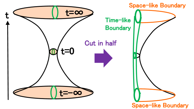
Figure 3: The left panel shows a sketch of global de Sitter space, which has only space-like boundaries at $t=\pm\infty$. The right one is a sketch of our holographic setup which is obtained by cutting in half a de Sitter space. Notice that this geometry has both the time-like and space-like boundary.

Case 1: Schwinger-Keldysh prescription without EOW

We apply the Hartle-Hawking prescription to construct the initial state at $t=0$ using the Euclidean instanton geometry, which takes the form of a $d+1$ dimensional semi-sphere. Subsequently, we examine its Lorentzian time evolution. The density matrix for this state at time $t$ is determined by the corresponding geometry dictated by the Schwinger-Keldysh prescription, as depicted in figure 4. For a detailed understanding of the Schwinger-Keldysh prescription in holography and holographic entanglement entropy, we refer readers to Skenderis:2008dg ; Dong:2016hjy . It is important to note that the asymptotic infinity as $t\to\infty$ is absent in this particular setup. In line with conventional Lorentzian holography in AdS, we anticipate that the gravitational dynamics in half dS_d+1 geometry is dual to a field theory residing on its boundary, namely, dS_d. We expect this field theory to exhibit strong non-locality, primarily due to the fact that the boundary at $\theta=\theta_{0}$ is not an asymptotic boundary. Unlike in the AdS/CFT correspondence, the metric, in this case, does not exhibit divergent behaviour, indicating that the dS boundary plays the role of a finite cutoff.

Case 2: Final state projection with EOW

On the other hand, if we consider the full geometry of a half dS_d+1, we need to impose a boundary condition at the infinity $t\to\infty$. If we impose the Dirichlet b.c., then we expect a dual CFT lives there in addition to the dS_d boundary. To avoid this complicated situation, we focus on the other case: Neumann boundary condition. Namely this means that the asymptotic boundary $t=\infty$ is an end-of-the-world (EOW) brane. In the context of AdS/CFT, the EOW brane is dual to the boundary conformal field theory (BCFT), whose holographic duality is called the AdS/BCFT Takayanagi:2011zk ; Fujita:2011fp ; Karch:2000gx . In our dS case, we expect that the dual theory is a non-local field theory on dS_d with a final state projection at future infinity $t=\infty$.

In the presence of post-selection, a useful quantity is pseudo entropy Nakata:2021ubr , which is a natural generalization of entanglement entropy such that it depends on two different quantum states $|\psi_{1}\rangle$ and $|\psi_{2}\rangle$. This quantity is defined as follows. We introduce the reduced transition matrix

$$\tau_{A}=\mbox{Tr}_{B}\left[\frac{|\psi_{1}\rangle\langle\psi_{2}|}{\langle\psi_{2}|\psi_{1}\rangle}\right].$$ (1.5)

The pseudo entropy is defined by

$$S_{A}=\mbox{Tr}\left[-\tau_{A}\log\tau_{A}\right].$$ (1.6)

Note that this quantity in general takes complex values as $\tau_{A}$ is not hermitian.

Interestingly, the gravity dual of this quantity is given by (1.3) when $\Gamma_{A}$ is the minimal surface in an Euclidean time-dependent asymptotically AdS Nakata:2021ubr . We can also regard the area of extremal surface as a holographic pseudo entropy in Lorentzian AdS in the presence of final state projection Akal:2021dqt . We will assume an extension of this correspondence to de Sitter spaces in this paper. As studies of quantum many-body systems and CFTs suggest Mollabashi:2020yie ; Mollabashi:2021xsd ; Akal:2021dqt the real part of pseudo entropy typically measures the amount of quantum entanglement in the intermediate states between $|\psi_{1}\rangle$ and $|\psi_{2}\rangle$.

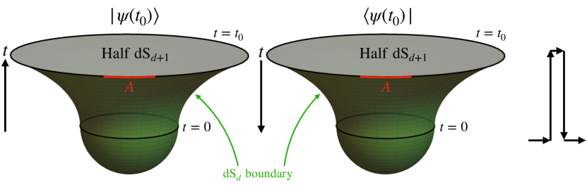
Figure 4: The geometry which describes the Schwinger-Keldysh contour of a half dS_d+1. The top and bottom region presents the Lorentzian and Euclidean evolution, respectively. This is dual to a field living on dS_d boundary which is parametrized by the green surface.

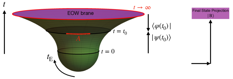
Figure 5: The geometry of a half dS_d+1. Notice that there are both timelike (green surface) and spacelike (purple surface) boundaries.

This paper is organized as follows. In section 2, we study the AdS/CFT for CFTs on de Sitter space. We calculate the entanglement entropy in both case 1 and case 2 and discuss physical interpretations. In section 3 we consider the holography for a half de Sitter space in case 1. We calculate the holographic entanglement entropy and study its property including the violation of subadditivity. We will discuss its implication on the Hilbert structure of its dual field theory. In section 4 we study the holographic duality for a half de Sitter space in case 2, taking into account the presence of EOW brane. In section 5 we summarize our conclusions and discuss future problems. In appendix A, we show explicit calculations of geodesics in de Sitter space.

2 CFT on de Sitter Space from AdS/CFT

Before we work on the holography of de Sitter spaces, we would like to examine the AdS/CFT correspondence with CFT living on the de Sitter space as a warm up exercise. In this section, we focus on the holographic CFT₂ living on dS₂ spacetime whose metric is defined by

$$\begin{split}ds^{2}_{\mathrm{dS}_{2}}=-dt^{2}+\cosh^{2}{t}d\phi^{2}=\frac{1}{\cos^{2}{T}}\left(-dT^{2}+d{\phi}^{2}\right)\,.\end{split}$$ (2.1)

In the following dS metrics, we have chosen the de Sitter radius to be a unit, and use the transformation between the global time $t$ and conformal time $T$ given by $\cosh{t}=\frac{1}{\cos{T}}$. We note that the conformal time is compactified due to $T\in[-\frac{\pi}{2},\frac{\pi}{2}]$, while the global time is not, i.e. $t\in(-\infty,+\infty)$.

For simplicity, we mainly consider AdS${}_{3}/$CFT₂ where the CFT lives on dS₂. The holographic dual is described by the global AdS₃,

$$ds^{2}_{(g)}=-\cosh^{2}\rho d\tau^{2}+d\rho^{2}+\sinh^{2}\rho d\phi^{2}\,.$$ (2.2)

where $\rho$ is the radial coordinate and $\tau$ is the global time coordinate of AdS bulk spacetime. Since the extremal surface in AdS₃ is nothing but a geodesic, we can evaluate the area of the extremal surface using the geodesic distance $D^{(g)}_{12}$ in the global AdS metric between two points $(\rho_{1},\tau_{1},\phi_{1})$ and $(\rho_{2},\tau_{2},\phi_{2})$, as given by

$$\cosh D^{(g)}_{12}=\cos(\tau_{1}-\tau_{2})\cosh\rho_{1}\cosh\rho_{2}-\cos(\phi_{1}-\phi_{2})\sinh\rho_{1}\sinh\rho_{2}\,.$$ (2.3)

2.1 de Sitter and Hyperbolic Slicing of AdS ₃

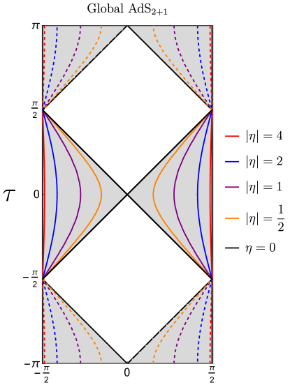
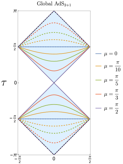
Figure 6: Left: Penrose diagram of AdS₃ with de Sitter slicing which is defined in eq. (2.4). The solid curves denote the constant $\eta$ surfaces with $\eta>0$ and the negative ones are described by the dashed curves. Right: Penrose diagram of AdS₃ with hyperbolic slicing as described by the metric (2.8). The solid and dashed curves present constant $\mu$ surfaces with positive and negative values, respectively.

To describe a CFT on dS₂, we employ the de Sitter sliced AdS₃ (refer to the left plot in figure 6):

$$ds^{2}_{(d)}=d\eta^{2}+\sinh^{2}\eta(-dt^{2}+\cosh^{2}td\phi^{2}),$$ (2.4)

where $(t,\eta)$ is related to the global coordinates $(\tau,\rho)$ via

$$\sinh\rho=\cosh t\sinh|\eta|,\ \ \ \ \tan\tau=\tanh\eta\,\sinh t\,$$ (2.5)

The coordinate transformation (2.5) leads to the geodesic length between two points $(t_{1},\eta_{1},\phi_{1})$ and $(t_{2},\eta_{2},\phi_{2})$ in the dS sliced metric:

$$\cosh D^{(d)}_{12}=\cosh\eta_{1}\cosh\eta_{2}-\sinh\eta_{1}\sinh\eta_{2}\left(\cosh t_{1}\cosh t_{2}\cos\left(\phi_{2}-\phi_{1}\right)-\sinh t_{1}\sinh t_{2}\right)\,.$$ (2.6)

The holographic CFT₂ on dS₂ with a physical metric (2.1) is living on the conformal boundary of AdS₃ which is defined by $\eta\to\infty$. We can fix the UV cut-off $\epsilon$ in the CFT₂ by taking the cut-off surface at $\eta=\eta_{\infty}$ with

$$e^{\eta_{\infty}}=\frac{1}{\tanh\frac{\epsilon}{2}}\approx\frac{2}{\epsilon}\,.$$ (2.7)

For a later purpose it is also useful to consider a hyperbolic sliced AdS₃ (refer to the right plot in figure 6), whose metric reads

$$ds^{2}_{(h)}=-d\mu^{2}+\cos^{2}\mu(d\xi^{2}+\sinh^{2}\xi d\phi^{2})\,.$$ (2.8)

The coordinate $(t,\eta)$ is related to that of the global AdS₃ $(\tau,\rho)$ via

$$\sinh\rho=\sinh\xi\cos\mu,\ \ \ \ \tan\tau=\cot\mu\,\cosh\xi,$$ (2.9)

The geodesic length $D^{(h)}_{12}$ between two points at $(\mu_{1},\xi_{1},\phi_{1})$ and $(\mu_{2},\xi_{2},\phi_{2})$ can be derived from

$$\cosh D^{(h)}_{12}=\cos\mu_{1}\cos\mu_{2}\left(\cosh\xi_{1}\cosh\xi_{2}-\cos(\phi_{1}-\phi_{2})\sinh\xi_{1}\sinh\xi_{2}\right)+\sin\mu_{1}\sin\mu_{2}\,.$$ (2.10)

It is also useful to note that the hyperbolic sliced metric and the de Sitter sliced one are related by the following analytical continuation:

$$\eta=i\left(\mu-\frac{\pi}{2}\right)\,,\qquad\xi=i\frac{\pi}{2}-t\,.$$ (2.11)

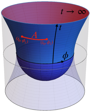
Figure 7: The setup of computing entanglement entropy of CFT₂ on dS₂ via AdS₃/CFT₂. We replace the region $t<0$ by the Euclidean instanton namely the half sphere, following Hartle-Hawking prescription (blue shaded region). In the case of Schwinger-Keldysh setup, we restrict the Lorentzian path-integral to the region $0\leq t\leq t_{0}$ and glue the same path-integral at $t=t_{0}$.

2.2 Case 1:Entanglement entropy in Schwinger-Keldysh prescription

In this section, we aim to compute the holographic entanglement entropy Ryu:2006bv ; Ryu:2006ef ; Hubeny:2007xt for a CFT living on dS₂ spacetime, following the Schwinger-Keldysh prescription (case 1) of the CFT on a time-dependent background. Refer to Maldacena:2012xp for calculations of holographic entanglement entropy for CFTs on de Sitter spaces in higher dimensions.

Specifically, we assume that the quantum state at $t=0$ is generated by an Euclidean path integral on a semi-sphere using the Hartle-Hawking prescription, as depicted in figure 7. To define the entanglement entropy $S_{A}$, we take the subsystem $A$ as an interval with endpoints $(t_{0},\phi_{1})$ and $(t_{0},\phi_{2})$, as shown in figure 7.

To derive the holographic entanglement entropy, we construct the gravity dual by gluing two copies of AdS₃, each truncated at a time $t=t_{0}$, following the holographic Schwinger-Keldysh prescription Skenderis:2008dg ; Dong:2016hjy . Hence, there is no need to consider the treatment of the conformal boundary of the dS₂ at $t=\infty$. Utilizing the geodesic length given in eq. (2.6), we can obtain the holographic entanglement entropy, viz,

$$S^{\rm con}_{A}=\frac{c}{3}\log\left[\frac{2\cosh t_{0}\sin\frac{|\phi_{1}-\phi_{2}|}{2}}{\epsilon}\right]\,,$$ (2.12)

where we adopt the cutoff surface specified by eq. (2.7). Notably, this entanglement entropy exhibits a linear growth as $S_{A}\simeq\frac{c}{3}t_{0}$ at late times. We attribute this contribution to a connected geodesic that connects two boundary points. Thus, in the Schwinger-Keldysh setup, this result (2.12) provides the final expression for the holographic entanglement entropy.

2.3 Case 2: Holographic pseudo entropy with a final state projection

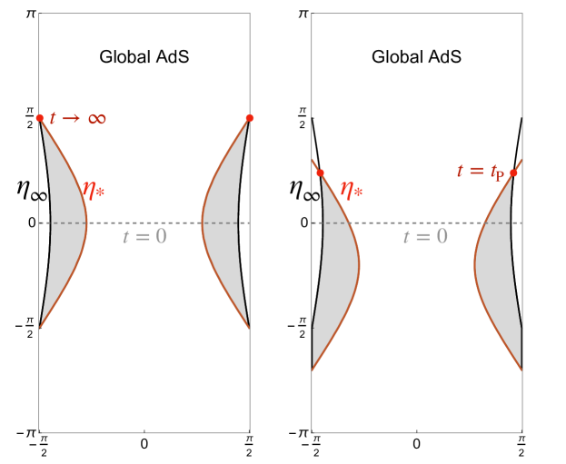
Figure 8: The holographic dual of CFT₂ living on dS₂ with a projection is shown as the gray shaded region. The angular direction of AdS₃ is not shown in this figure. The solid black curve represents the two dimensional dS spacetime where CFT₂ lives. Left: The projection is performed at the infinity time $t_{\textrm{\tiny P}}\to\infty$ with a dS₂ brane (red curve) parametrized by a constant $\eta_{\ast}$. Right: The projection at a finite time $t_{\textrm{\tiny P}}$.

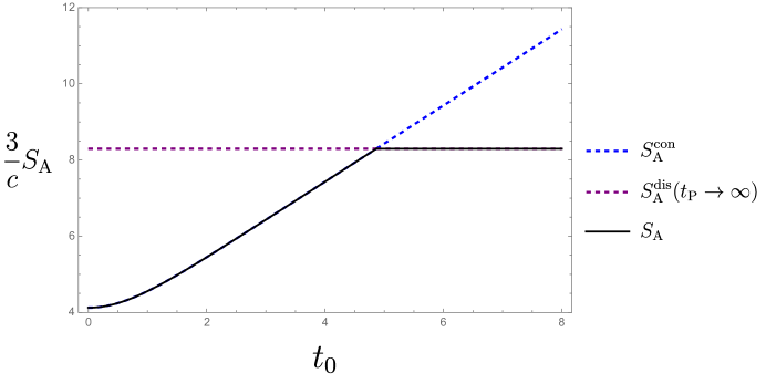
Figure 9: The plot of $S^{\rm con}_{A}$ (blue) and $S^{\rm dis}_{A}$ (purple) as a function of time $t$. We set $\eta_{\ast}=3,\phi_{2}-\phi_{1}=\frac{\pi}{5},\epsilon=\frac{1}{100}$ for this numerical plot.

We now consider the setup in which there is a final state projection with a boundary state $|\rm{B}\rangle$ at future infinity $t=\infty$, and interpret the area of the extremal surface, i.e., $S_{A}$ as the holographic pseudo entropy Nakata:2021ubr . To construct the gravity dual of the holographic CFT₂ with a projection, we insert an end-of-the-world brane (EOW) brane on which we impose Neumann boundary condition, i.e.,

$$K_{ij}-Kh_{ij}+Th_{ij}=0\,,\qquad\text{with}\qquad K=2T\,,$$ (2.13)

where $K_{ij}$ is the extrinsic curvature of the brane and the constant $T$ is the brane tension. Since the bulk is AdS₃ spacetime, one can show that the solutions of eq. (2.13) have to be maximally symmetric spacetime as well. More explicitly, one can obtain (see e.g., Kawamoto:2023wzj )

$$R_{ij}[h]=h_{ij}\left(\varepsilon\,T^{2}-1\right)\,,\qquad\text{with}\quad R[h]=2(\varepsilon\,T^{2}-1)\,,$$ (2.14)

for a timelike brane with $\varepsilon=+1$ and a spacelike brane with $\varepsilon=-1$, respectively. In order words, the intrinsic geometry of the brane is nothing but two dimensional Minkowski ($|T|=1$), de Sitter ($|T|>1$), AdS ($|T|<1$) spacetime or hyperbolic space ($\varepsilon=-1$). The de Sitter EOW brane in AdS/BCFT was introduced in Akal:2020wfl and was applied to the calculation of holographic pseudo entropy in Akal:2021dqt in the context of black hole final state proposal Horowitz:2003he .

With taking the intersection of the brane and the dS₂ boundary at $t\to\infty$, we can find that there are two types of solutions of the brane: a timelike dS brane and a spacelike hyperbolic brane. From the dS slicing and hyperbolic slicing of AdS₃, one can easily read the corresponding brane profiles in global AdS₃ (as shown in figure 6), i.e.,

$$\begin{split}\text{dS${}_{2}$ brane:}\qquad\cosh\rho\cos\tau&=\pm\cosh\eta_{\ast}\,,\\ \text{H${}_{2}$ brane:}\qquad\cosh\rho\cos\tau&=\sin\mu_{\ast}\,,\\ \end{split}$$ (2.15)

where $\eta_{\ast},\mu_{\ast}$ is a constant along the brane and is determined by the tension which is given by the boundary entropy of the boundary state. Furthermore, the parameter $\eta_{\ast}$ and $\mu_{\ast}$ should be determined by the boundary condition at $t=\infty$.

We begin with the case with a dS₂ EOW brane. Let us first note that the trace of the extrinsic curvature of EOW brane can be expressed as follows:

$$K\big{|}_{\eta=\eta_{\ast}}=-\frac{\partial_{\eta}\sqrt{-\gamma}}{\sqrt{-\gamma}}\Big{|}_{\eta=\eta_{\ast}}=-\frac{2\cosh\eta_{\ast}}{\sinh\eta_{\ast}}\,,$$ (2.16)

which indicates that the tension and curvature of the EOW brane are given by $T=-\coth\eta_{\ast}<0$ and $R=\frac{2}{\sinh^{2}\eta_{\ast}}$, respectively. The corresponding boundary entropy associated with the boundary state $\ket{B}$ projected at $t\to\infty$ can be calculated as Akal:2021dqt

$$S_{\rm bdy}=\frac{c}{6}\log\sqrt{\frac{1-\mathcal{T}}{1+\mathcal{T}}}=\frac{c}{6}\log\sqrt{\frac{|\mathcal{T}|-1}{|\mathcal{T}|+1}}-i\,\frac{\pi c}{12}=-\frac{c}{6}\eta_{\ast}-i\,\frac{\pi c}{12}\,.$$ (2.17)

which decodes the information of the boundary condition at $t\to\infty$.

Due to the appearance of the EOW brane in the bulk, we must account for the disconnected geodesic that connects a endpoint $(t_{0},\eta_{\infty},\phi_{i})$ of boundary interval $A$ to a point $(t_{\ast},\eta_{\ast},\phi_{\ast})$ on the de Sitter EOW brane. Thanks to the rotation invariance, it is straightforward to get the extremal surface is given by $\phi_{\ast}=\phi_{i}$. Furthermore, we can fix the coordinate values of $t_{\ast}$ on the brane by ensuring that the geodesic length remains stationary. For the de Sitter EOW brane, the disconnected contribution for pseudo entropy can be derived from eq. (2.6) as follows:

$$S^{\rm dis}_{A}=\frac{c}{3}(\eta_{\infty}-\eta_{\ast})=\frac{c}{3}\log\frac{2}{\epsilon}-\frac{c}{3}\eta_{\ast}\,$$ (2.18)

where the constant part is the real part of the boundary entropy defined in eq. (2.17).

If we compare the connected contribution $S^{\rm con}_{A}$ and the disconnected part $S^{\rm dis}_{A}$, we find that in the early time $S^{\rm con}_{A}$ is favored and holographic pseudo entropy of the interval $A$ grows linearly in time. However, $S^{d\rm dis}_{A}$ is always favored in the late time and holographic pseudo entropy becomes a constant. This phase transition is plotted in figure 9. At $\eta_{\ast}=0$, this phase transition happens when

$$\cosh t_{0}\cdot\sin\frac{|\phi_{1}-\phi_{2}|}{2}=1.$$ (2.19)

This describes the null geodesic in dS₂ as sketched in figure 14, which is the same as (3.10).

For the hyperbolic EOW brane, the disconnected PE is estimated from (2.6) as follows:

$$S^{\rm dis}_{A}=\frac{c}{3}\log\frac{2}{\epsilon}+i\frac{c}{3}\left(\frac{\pi}{2}-\mu_{*}\right),$$ (2.20)

where $\mu_{*}$ takes the range $-\frac{\pi}{2}\leq\mu_{*}\leq\frac{\pi}{2}$.

Before we go on, we would like to mention a possibility that this holographic calculation of pseudo entropy may actually be interpreted as genuine entanglement entropy. This is because the global AdS₃ has the periodicity in the time direction $\tau$. This may imply the periodicity for the time evolution by $\pi$ of the boundary state $e^{-i\pi H}|\text{B}\rangle\propto|\text{B}\rangle$. Even though this is suggested by the classical geometry, we are not completely sure if this is true at the quantum level which is dual to the full dynamics of the CFT. We leave this issue for a future problem.

2.4 Holographic pseudo entropy under final state projection at $t=t_{\textrm{\tiny P}}$

For later purpose, it is useful to consider a CFT on dS₂ with a final state projection at a finite time $t=t_{\textrm{\tiny P}}$. In the AdS${}_{3}/$BCFT₂, this is dual to inserting the EOW brane earlier as depicted in the right panel of figure 8. It is obvious that $S_{A}$ vanishes at $t=t_{\textrm{\tiny P}}$. Therefore the time evolution of $S_{A}$ looks like a Page curve as sketched in the right panel of figure 10.

Since the brane profile is not completely covered by the dS slicing coordinates, it is more convenient to work on the global coordinates (2.2). We denote the points on the dS boundary as $(\tau_{0},\rho_{\infty},\phi_{0})$. The dS boundary is thus given by

$$\cosh\rho_{\infty}\cos\tau_{0}=\text{constant}=\cosh\eta_{\infty}\,,$$ (2.21)

where $\eta_{\infty}$ determines the position of the dS boundary. Corresponding, the point on the brane is referred to as $(\tau_{*},\rho_{*},\phi_{*})$. Since the brane is still represents a two-dimensional dS spacetime, we can parametrize the brane profile as

$$\cosh\rho_{*}\cos\left(\tau_{*}+\tau_{\rm shift}\right)=\text{constant}=\cosh\eta_{\ast}\,,$$ (2.22)

where $\eta_{\ast}$ is related to the tension of the brane. Since we parametrize the projection time is $t=t_{\textrm{\tiny P}}$ or $T=T_{\textrm{\tiny P}}$ in terms of the time coordinate on the dS boundary, we can find that this fix the brane parameter $\tau_{\rm shift}$ as

$$\tau_{\rm shift}=\arccos\left(\frac{\cosh\eta_{\ast}\cos T_{0}}{\cosh\eta_{\infty}}\right)-\tau{\textrm{\tiny P}}=\arccos\left(\frac{\cosh\eta_{\ast}\cos T_{0}}{\cosh\eta_{\infty}}\right)-\arctan\left(\tanh\eta_{\infty}\tan T_{\textrm{\tiny P}}\right)\,,$$ (2.23)

with using the coordinate transformations for the points on dS boundary as

$$\begin{cases}\cosh\rho=\sqrt{\cosh^{2}\eta+\sinh^{2}\eta\tan^{2}T}\,,\\ \tan\tau=\tanh\eta\tan T\,.\\ \end{cases}$$ (2.24)

On the other hand, the geodesic distance $D_{0b}$ from the dS boundary to dS brane is derived as

$$\cosh D_{0b}=\cos(\tau_{0}-\tau_{*})\cosh\rho_{\infty}\cosh\rho_{*}-\cos(\phi_{0}-\phi_{*})\sinh\rho_{\infty}\sinh\rho_{*}.$$ (2.25)

Extremization over the spatial direction simply results in $\phi_{0}=\phi_{*}$, which is expected by symmetries. Furthermore, we need to find that maximal value over the timelike direction by solving

$$\frac{\partial D_{0b}}{\partial\tau_{*}}=0\,,\quad\text{with}\quad\rho_{*}=\rho_{*}(\tau_{*})\,,$$ (2.26)

which reduces to

$$\cosh\eta_{\ast}\sinh\rho_{\infty}\tan\left(\tau_{*}+\tau_{\rm shift}\right)-\frac{\sin\left(\tau_{*}+\tau_{\rm shift}\right)}{\cos\left(\tau_{0}+\tau_{\rm shift}\right)}\cosh\rho_{\infty}\sqrt{\cosh^{2}\eta_{\ast}-\cos^{2}\left(\tau_{0}+\tau_{\rm shift}\right)}=0\,.$$ (2.27)

The advantage of working on global coordinates is obvious in the above extremization equation. After straightforward algebras, one can derive the solutions as

$$\begin{split}\cos\left(\tau_{*}+\tau_{\rm shift}\right)&=\cosh\eta_{\ast}\sqrt{\frac{\cosh^{2}\rho_{\infty}\sin^{2}(\tau_{0}+\tau_{\rm shift})-\sinh^{2}\rho_{\infty}}{\cosh^{2}\rho_{\infty}\sin^{2}(\tau_{0}+\tau_{\rm shift})-\sinh^{2}\rho_{\infty}\cosh^{2}\eta_{\ast}}}\,,\\ \cosh\rho_{*}&=\sqrt{\frac{\cosh^{2}\rho_{\infty}\sin^{2}(\tau_{0}+\tau_{\rm shift})-\sinh^{2}\rho_{\infty}\cosh^{2}\eta_{\ast}}{\cosh^{2}\rho_{\infty}\sin^{2}(\tau_{0}+\tau_{\rm shift})-\sinh^{2}\rho_{\infty}}}\,.\\ \end{split}$$ (2.28)

Substituting the above solutions to the expression for the distance of geodesics, we can obtain the distance of the extremal geodesic between the dS boundary and brane, i.e., the area of the disconnected HRT surface.

We are interested in the case where the dS boundary is taken as the cut-off surface located at $\eta_{\infty}\sim\frac{2}{\epsilon}$. In this limit, we can rewrite the global coordinates on the boundary as

$$\begin{split}\tau_{0}&=T_{0}\,,\qquad\rho_{\infty}\approx\log\left(\frac{2}{\epsilon\cos T_{0}}\right)\,,\qquad\tau_{\rm shift}=\frac{\pi}{2}-T_{\textrm{\tiny P}}\,.\\ \end{split}$$ (2.29)

The extremal point on the brane reduces to

$$\begin{split}\sin\left(T_{\textrm{\tiny P}}-\tau_{*}\right)&=\cosh\eta_{\ast}\sqrt{\frac{\sin^{2}(T_{\textrm{\tiny P}}-T_{0})}{\cosh^{2}\eta_{\ast}-\cos^{2}(T_{\textrm{\tiny P}}-T_{0})}}\,,\\ \cosh\rho_{*}&=\sqrt{1+\frac{\sinh^{2}\eta_{\ast}}{\sin^{2}(T_{\textrm{\tiny P}}-T_{0})}}\,,\\ \end{split}$$ (2.30)

and the corresponding geodesic distance is given by

$$D_{0b}\approx\log\left(\frac{2}{\epsilon}\frac{\cos(T_{0}+\tau_{\rm shift})}{\cos T_{0}}e^{-\eta_{\ast}}\right)\,.$$ (2.31)

Thus, the holographic entanglement entropy from the disconnected HRT surface is recast as

$$S^{\rm dis}_{A}=\frac{2D_{0b}}{4G_{\textrm{\tiny N}}}=\frac{c}{3}\log\left(\frac{2}{\epsilon}\frac{\sin\left(T_{\textrm{\tiny P}}-T_{0}\right)}{\cos T_{0}}\right)-\frac{c}{3}\eta_{\ast}\,.$$ (2.32)

In terms of the de Sitter time $t$, we finally find the following expression:

$$S^{\rm dis}_{A}=\frac{c}{3}\log\left[\frac{2}{\epsilon}\cdot\frac{\sinh t_{\textrm{\tiny P}}-\sinh t_{0}}{\cosh t_{\textrm{\tiny P}}}\right]-\frac{c}{3}\eta_{\ast},$$ (2.33)

where we have used $\sinh t_{\textrm{\tiny P}}=\tan T_{\textrm{\tiny P}}$. The holographic pseudo entropy in the presence of final state projection is given by the smaller one among the two: $S_{A}=\mbox{min}[S^{\mathrm{con}}_{A},S^{\mathrm{dis}}_{A}]$.

2.5 Entanglement/Pseudo entropy of CFT₂ on dS₂

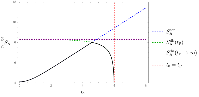
Figure 10: Time evolution of holographic entanglement entropy (denoted by the black curve) with respect to the global time $t_{0}$. The projection time is chosen as $t_{\textrm{\tiny P}}=6$ with $\eta_{\ast}=3$. We set $\phi_{2}-\phi_{1}=\frac{\pi}{5},\epsilon=\frac{1}{100}$ for this numerical plot.

It is intriguing to compare previous holographic results of entanglement entropy and pseudo entropy with that derived in 2d CFT. Indeed, as in the general replica method for 2d CFTs Holzhey:1994we ; Calabrese:2004eu , we can easily compute the two-point function of twist operators of local CFT on the $\mathrm{dS}_{2}$ by considering the Weyl scaling:

$$\langle\sigma(t_{0},\phi_{1})\overline{\sigma}(t_{0},\phi_{2})\rangle_{\mathrm{dS}_{2}}=(\cos{T_{0}})^{2\Delta_{n}}\langle\sigma(T_{0},\phi_{1})\overline{\sigma}(T_{0},\phi_{2})\rangle_{\mathrm{cylinder}}\,.$$ (2.34)

Here we have define the conformal coordinates $(T,\phi)$ by

$$\begin{split}ds^{2}_{\mathrm{dS}_{2}}&=-dt^{2}+\cosh^{2}{t}d\phi^{2}=\frac{1}{\cos^{2}{T}}\left(-dT^{2}+d{\phi}^{2}\right)\,\\ \end{split}$$ (2.35)

with the transformation between the global time and conformal time given by $\cosh{t}=\frac{1}{\cos{T}}$. The Euclidean part of the Hartle-Hawking state is described by a half sphere whose metric reads

$$ds^{2}_{\mathrm{HH}}=dt_{\textrm{\tiny E}}^{2}+\cos^{2}{t_{\textrm{\tiny E}}}d\phi^{2}=\frac{1}{\cosh^{2}T_{\textrm{\tiny E}}}\left(dT_{\textrm{\tiny E}}^{2}+d{\phi}^{2}\right)\,,$$ (2.36)

where the Euclidean conformal time $T_{\textrm{\tiny E}}$ is defined by $\cos{t_{\textrm{\tiny E}}}=\frac{1}{\cosh{T_{\textrm{\tiny E}}}}$ with $-\frac{\pi}{2}\leq t_{\textrm{\tiny E}}\leq 0,-\infty\leq T_{\textrm{\tiny E}}\leq 0$.

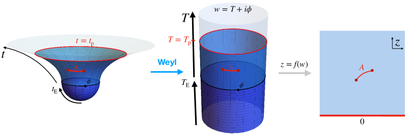
Figure 11: The conformal maps used for computing the pseudo entropy. The projection is performed at a fixed time $t_{\textrm{\tiny P}}$ which is indicated by the red circle.

Case 1: Schwinger-Keldysh description without EOW

First of all, it is known that the entanglement entropy for an interval in the cylinder is shown as

$$S_{A}^{\mathrm{cylinder}}=\frac{c}{3}\log{\left(\frac{2}{\epsilon}\sin{\frac{|\phi_{1}-\phi_{2}|}{2}}\right)}\,.$$ (2.37)

where we have used the fact that the periodicity of the cylinder is $2\pi$. Noting the contribution from Weyl scaling, we can obtain

$$S_{A}^{\mathrm{dS}_{2}}=\frac{c}{3}\log{\cosh{t_{0}}}+\frac{c}{3}\log{\left(\frac{2}{\epsilon}\sin{\frac{|\phi_{1}-\phi_{2}|}{2}}\right)}\,,$$ (2.38)

which reproduces the holographic result shown in eq. (2.12).

Case 2: Final projection at $t=t_{\textrm{\tiny P}}$

To compute the pseudo entropy of CFT₂ living on $\mathrm{dS}_{2}$, we follow the recipe illustrated in figure 11. Let us begin with the following two-point function and its Weyl scaling:

$$\begin{split}&\bra{\rm B}e^{iH(T_{p}-T)}\sigma(T_{0},\phi_{1})\overline{\sigma}(T_{0},\phi_{2})\ket{\rm HH}_{\mathrm{dS}_{2}}\\ =&(\cos{T_{0}})^{2\Delta_{n}}\bra{\rm B}e^{-iH(T_{\textrm{\tiny P}}-T)}\sigma(T_{0},\phi_{1})\overline{\sigma}(T_{0},\phi_{2})\ket{0}_{\mathrm{cylinder}}\,,\end{split}$$ (2.39)

where $|\rm B\rangle$ is the boundary state (Cardy state) in the boundary conformal field theory (BCFT) Cardy:2004hm and $|\rm HH\rangle$ denotes the Hartle-Hawking state of dS₂. We can first focus on the transition matrix, i.e.,

$$\bra{\rm B}e^{-iH(T_{\textrm{\tiny P}}-T)}\sigma(T_{0},\phi_{1})\overline{\sigma}(T_{0},\phi_{2})\ket{0}_{\mathrm{cylinder}}\,,$$ (2.40)

with ignoring the Weyl factor. The corresponding cylinder for evaluating the transition matrix is composed of the infinitely long Euclidean cylinder $-\infty\leq T_{\textrm{\tiny E}}\leq 0$ and also a finite Lorentzian cylinder with $0\leq T\leq T_{\textrm{\tiny P}}$. By Wick rotation, we consider the Euclidean cylinder $-\infty\leq T_{\textrm{\tiny E}}\leq T_{\textrm{\tiny P}}^{E}=iT_{\textrm{\tiny P}}$. With denoting the complex coordinate for the cylinder as

$$w=T_{\textrm{\tiny E}}+i\phi\,,$$ (2.41)

we can map the Euclidean cylinder to the upper half plane. The explicit conformal map is given by

$$\frac{e^{w}}{e^{T_{\textrm{\tiny P}}^{E}}}=\frac{z-i}{z+i}\Leftrightarrow z=f(w)=-i\frac{e^{w-T_{\textrm{\tiny P}}^{E}}+1}{e^{w-T_{\textrm{\tiny P}}^{E}}-1}\,.$$ (2.42)

See the figure 11 for the illustration.

By assuming the mirror trick and the factorization, it is straightforward to evaluate the transition (2.40). Similar to the connected and disconnected geodesics, one can also obtain two distinct contributions, i.e.,

1. Connected part:

   $$S^{\mathrm{con,cyl}}_{A}=\frac{c}{6}\log\frac{|f(w_{1})-f(w_{2})|^{2}}{\epsilon^{2}|f^{\prime}(w_{1})||f^{\prime}(w_{2})|}.$$ (2.43)

   After substituting

   $$w_{1}=i(T_{0}+\phi_{1}),w_{1}^{*}=i(T_{0}-\phi_{1}),w_{2}=i(T_{0}+\phi_{2}),w_{2}^{*}=i(T_{0}-\phi_{2})\,,$$ (2.44)

   we obtain the same formula (2.38) which it was derived in holographic spacetime for Case 1.

2. Disconnected part:

   $$S^{\mathrm{dis,cyl}}_{A}=\frac{c}{6}\log\frac{|f(w_{1})-\bar{f}(\bar{w}_{1})||f(w_{2})-\bar{f}(\bar{w}_{2})|}{\epsilon^{2}|f^{\prime}(w_{1})||f^{\prime}(w_{2})|}+2S_{\mathrm{bdy}}.$$ (2.45)

   Again, by substituting eq. (2.44), we can derive the contribution from the disconnected part, viz,

   $$S^{\mathrm{dis,cyl}}_{A}=\frac{c}{6}\log{\frac{-4}{\epsilon^{2}}\sin^{2}{(T_{p}-T_{0})}}+2S_{\mathrm{bdy}}=\frac{c}{3}\log\left(\frac{2}{\epsilon}\sin{(T_{p}-T_{0})}\right)+\frac{\pi i}{12}c+2S_{\mathrm{bdy}}\,.$$ (2.46)

   Finally, we need to consider the extra contribution from Weyl scaling and rewrite the final answer as

   $$S_{A}^{\mathrm{dis,dS}}=\frac{c}{3}\log\left(\frac{2}{\epsilon}\frac{\sin{(T_{p}-T_{0})}}{\cos{T_{0}}}\right)+\frac{\pi i}{12}c+2S_{\mathrm{bdy}}\,.$$ (2.47)

   Combining the two distinct results, we can also find that the pseudo entropy present the same behavior as shown in figure 10. Especially, when the post-selection is fixed at the future infinity, i.e., $T_{p}=\frac{\pi}{2}$, the disconnected part reduces to a constant

   $$S_{A}^{\mathrm{dis,dS}}=\frac{c}{3}\log\left(\frac{2}{\epsilon}\right)+\frac{\pi i}{12}c+2S_{\mathrm{bdy}}\,,$$ (2.48)

As a summary, we find that pseudo entropy derived from boundary 2d CFT agree with the holographic results for $S^{dis}_{A}$ (2.18) and (2.33) via the prescription (2.17).

2.6 Holographic entanglement in higher dimensions

In this section, we study the holographic entanglement (pseudo) entropy in higher dimensional setups, which can be found from the area of extremal surfaces in the $(d+1)$-dim AdS space. The de Sitter sliced metric is given by

$$ds^{2}=d\eta^{2}+\sinh^{2}\eta(-dt^{2}+\cosh^{2}t(d\phi^{2}+\sin^{2}\phi d\Omega_{d-2})).$$ (2.49)

Case 1: Schwinger-Keldysh without EOW

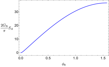
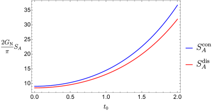
Figure 12: Holographic entanglement entropy $S^{\rm con}_{A}$ (2.56) and $S^{\rm dis}_{A}$ (2.61) from Schwinger-Keldysh prescription without EOW brane. We choose $d=3,\phi_{0}=\frac{\pi}{2},\eta_{\infty}=3$ and $\eta_{*}=1$for both plots.

First let us evaluate the connected entropy $S^{con}_{A}$. We consider the global AdS coordinates

$$ds^{2}=d\rho^{2}-\cosh^{2}\rho d\tau^{2}+\sinh^{2}\rho(d\phi^{2}+\sin^{2}\phi d\Omega_{d-2}^{2})$$ (2.50)

and take the subsystem $A$ as

$$0\leq\phi\leq\phi_{0},\quad\tau=\tau_{0},\quad\rho=\rho_{\infty}.$$ (2.51)

In this coordinate, the extremal surface is labeled by $\phi=\phi(\rho)$. The holographic entanglement entropy is the area of this surface divided by $4G_{N}$

$$S^{\rm con}_{A}=\frac{\mathrm{Vol}(\mathrm{S}^{d-2})}{4G_{N}}\int d\rho\sqrt{1+\sinh^{2}\rho\phi^{{}^{\prime}2}}(\sinh\rho\sin\phi)^{d-2},$$ (2.52)

where we set $\phi^{\prime}=\frac{\partial\phi}{\partial\rho}$. By taking the variation, we obtain the Euler-Lagrange equation

$$\phi^{\prime\prime}-\frac{d-2}{\tan\phi\sinh^{2}\rho}+\frac{d\phi^{\prime}}{\tanh\rho}-\frac{(d-2)\phi^{{}^{\prime}2}}{\tan\phi}+(d-1)\sinh\rho\cosh\rho\phi^{{}^{\prime}3}=0.$$ (2.53)

We find a suitable solution $\tanh\rho\cos\phi=C,$ where the $C$ is integration constant. We impose the boundary condition (2.51) and obtain the solution

$$\tanh\rho\cos\phi=\tanh\rho_{\infty}\cos\phi_{0}.$$ (2.54)

Then, the holographic entanglement entropy reads

$$S^{\rm con}_{A}=\frac{\mathrm{Vol}(\mathrm{S}^{d-2})}{4G_{N}}\int_{1}^{\frac{\cosh\rho_{\infty}}{\cosh\rho_{\rm min}}}du(u^{2}-1)^{\frac{d-3}{2}}\,,$$ (2.55)

where $\rho_{\rm min}$ is defined by $\tanh\rho_{\rm min}=\tanh\rho_{\infty}\cos\phi_{0}$. In particular, $S^{\rm con}_{A}$ for $d=3$ reduces to

$$\begin{split}S^{\rm con}_{A}=\frac{\pi}{2G_{N}}\left(\frac{\cosh\rho_{\infty}}{\cosh\rho_{\rm min}}-1\right)&=\frac{\pi}{2G_{N}}\left(\sqrt{\cosh^{2}t_{0}\sin^{2}\phi_{0}\sinh^{2}\eta_{\infty}+1}-1\right)\\ &\approx\frac{\pi}{2G_{N}}\left(\frac{\cosh t_{0}\sin\phi_{0}}{\epsilon}-1\right)\,,\\ \end{split}$$ (2.56)

We plot this as a function of $t_{0}$ and $\phi_{0}$ in figure 12.

Case 2: Final projection at $t=\infty$

Next, let us evaluate the disconnected extremal surfaces stretching between the dS boundary and the dS EOW brane, which contributes to the holographic pseudo entropy. Particularly, we consider the extremal surface connecting the two points between $(\eta_{\infty},t_{0},\phi_{0},\Omega_{0})$ and $(\eta_{*},t_{*},\phi_{*},\Omega_{0})$ and then maximize the area by taking variation with respect to $t_{*}$. In the AdS₃ case, the extremal surface satisfies $t=$const and $\phi$=const. However, in higher-dimensional cases this is no more true. Suppose that $\phi_{*}=\frac{\pi}{2}$ along the extremal surface. Then, its area is given by

$$S^{\rm dis}_{A}=\frac{\mathrm{Vol}(\mathrm{S}^{d-2})}{4G_{N}}\int d\eta\sqrt{1-\sinh^{2}\eta t^{{}^{\prime}2}}(\sinh\eta\cosh t)^{d-2}.$$ (2.57)

The Euler-Lagrange equation reads

$$\frac{(d-2)\tanh t}{\sinh^{3}\eta}+\frac{dt^{\prime}}{\tanh\eta\sinh\eta}-\frac{(d-2)\tanh tt^{{}^{\prime}2}}{\sinh\eta}-(d-1)\cosh\eta t^{{}^{\prime}3}+\frac{t^{\prime\prime}}{\sinh\eta}=0.$$ (2.58)

A particular solution, which is the one at $\tau=$const. in the global AdS, reads

$$\tanh\eta\sinh t=\tanh\eta_{\infty}\sinh t_{0}=\tanh\eta_{*}\sinh t_{*}.$$ (2.59)

We expect more general solutions and we need to maximize the areas of such solutions with respect to the end points on the EOW brane. However, this is highly complicated and we will focus on the above simple solution, which gives the minimal value of S${}_{A}^{\rm dis}$.

By substituting this into the functional we obtain

$$S_{A}^{\rm dis} =\frac{\mathrm{Vol}(\mathrm{S}^{d-2})}{4G_{N}}\int d\eta\sqrt{1-\sinh^{2}\eta t^{{}^{\prime}2}}(\sinh\eta\cosh t)^{d-2}$$

$$=\frac{\mathrm{Vol}(\mathrm{S}^{d-2})}{4G_{N}}\int^{\sqrt{1+\cosh^{2}t_{0}\sinh^{2}\eta_{\infty}}}_{\sqrt{1+\cosh^{2}t_{*}\sinh^{2}\eta_{*}}}dv(v^{2}-1)^{\frac{d-3}{2}}.$$ (2.60)

Especially, in the $d=3$ case we find

$$S_{A}^{\rm dis}=\frac{\pi\sqrt{\tanh^{2}\eta_{\infty}\sinh^{2}t_{0}+1}}{2G_{N}}(\cosh\eta_{\infty}-\cosh\eta_{*})\simeq\frac{\pi}{2G_{N}}\cosh t_{0}\left(\frac{1}{\epsilon}-\cosh\eta_{\ast}\right)\,,$$ (2.61)

The results are plotted in the figure 12. Unlike the AdS₃ case, both $S_{A}^{\rm con}$ and $S_{A}^{\rm dis}$ diverge exponentially as a function of $t_{0}$. Comparing two expressions in eqs. (2.56) and (2.61), we always have

$$S_{A}^{\rm dis}\leq S_{A}^{\rm con}\,,$$ (2.62)

due to $\cosh X\geq 1$.

More on Case 2: Final projection at $t=t_{\textrm{\tiny P}}$

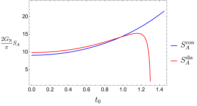
Figure 13: The time evolution of $S^{\rm con}_{A}$ (2.56) and $S^{\rm dis}_{A}$ (2.64). We take $\eta_{\infty}=3$, $\phi_{0}=\frac{\pi}{2}$ , $\tau_{\rm shift}=\frac{\pi}{6}$ and $\cosh\eta_{c}=0.2$. At early times, the connected part is dominated. After the phase transition, the disconnected part is dominated and approaches zero at the projection time $t_{0}=t_{\textrm{\tiny P}}$ , where the two branes intersect.

Next, we consider the final projection at finite time. For this, we shift the projection brane along the global time as in the section 2.4. If we shift the brane backward in $\tau_{\rm shift}$, the projection brane is defined by $\cosh\rho\cos(\tau+\tau_{\rm shift})=\cosh\eta_{c},$ where $\eta_{c}$ is related with the tension of the dS brane. The special solution to the extremal surface condition is already obtained in the previous section as (2.59) for $\phi_{0}=\frac{\pi}{2}$. Therefore the intersection of the extremal surface and the projection brane defines the end point of the surface $\tanh\eta_{*}\sinh t_{*}=\tanh\eta_{\infty}\sinh t_{0}$ and $\cosh\rho_{*}\cos(\tau_{*}+\tau_{\rm shift})=\cosh\eta_{c}.$

After short algebra we obtain

$$\cosh\eta_{*}=\frac{\cosh\eta_{c}}{\cos\tau_{\rm shift}-\tanh\eta_{\infty}\sinh t_{0}\sin\tau_{\rm shift}},$$ (2.63)

which gives for $d=3$

$$S^{\rm dis}_{A}=\frac{\pi\sqrt{\tanh^{2}\eta_{\infty}\sinh^{2}t_{0}+1}}{2G_{N}}\left(\cosh\eta_{\infty}-\frac{\cosh\eta_{c}}{\cos\tau_{\rm shift}-\tanh\eta_{\infty}\sinh t_{0}\sin\tau_{\rm shift}}\right)\,.$$ (2.64)

The figure 13 shows the plots. As in the AdS₃ case, the disconnected entropy reaches zero at the projection time $t_{\textrm{\tiny P}}$.

3 Holography for a half dS without EOW brane (Case 1)

Now we would like to move on to the our main target: holography with a positive cosmological constant. In order to interpret the holography in de Sitter space as in the standard framework where the bulk gravity is dual to a quantum system on its time-like boundary, we focus on a half of de Sitter space defined by restricting the global dS_d+1 given by the metric (1.1) and (1.2) to the region

$$0\leq\theta\leq\theta_{0},$$ (3.1)

as depicted in figure 2 and figure 3. The standard idea of holographic principle predicts that the bulk gravity on the half dS_d+1 (3.1) is dual to a certain quantum system on its boundary, namely, dS_d at $\theta=\theta_{0}$, given by the metric (1.4). We assume the range $0\leq\theta_{0}\leq\frac{\pi}{2}$. If we choose $\theta_{0}=\frac{\pi}{2}$ in particular, it is exactly a half of the original dS.

Below we will study how the holography for a half dS looks like by analyzing the holographic entanglement entropy. For simplicity we will mainly focus on the three dimensional space i.e. dS₃. In this case, the holographic entanglement entropy $S_{A}$, defined for an interval $A$, can be computed from the geodesic length which connects two end points of $A$. This consideration also suggests the range $0\leq\theta_{0}\leq\frac{\pi}{2}$. This is because the geodesics which compute the holographic entanglement entropy are not included in the half dS if $\theta_{0}\geq\frac{\pi}{2}$, even if the subsystem is very small.

3.1 Geodesic Length in dS₃

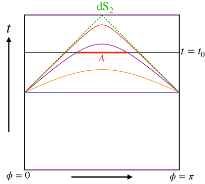
Figure 14: The Penrose diagram of dS₂ boundary. The colorful curves denote various spacelike geodesics on dS₂ where the null geodesic is presented by the green dashed curves.

To prepare for our analysis of holographic entanglement entropy $S_{A}$, let us see the behavior of the geodesics in a dS₃ whose metric reads

$$ds^{2}=-dt^{2}+\cosh^{2}t(d\theta^{2}+\sin^{2}\theta d\phi^{2}).$$ (3.2)

If we choose two points $P_{1}$ and $P_{2}$ on dS₃:

$$P_{1}=(t_{1},\theta_{1},\phi_{1})\,,\qquad P_{2}=(t_{2},\theta_{2},\phi_{2})\,,$$ (3.3)

then the geodesic distance between $P_{1}$ and $P_{2}$, denoted by $D_{12}$, can be found as

$$D_{12}=\left(\cos\theta_{1}\cos\theta_{2}+\sin\theta_{1}\sin\theta_{2}\cos(\phi_{1}-\phi_{2})\right)\cosh t_{1}\cosh t_{2}-\sinh t_{1}\sinh t_{2}\,.$$ (3.4)

Especially for the geodesic which connected two points $\phi=\phi_{1}$ and $\phi=\phi_{2}$ at the boundary $\theta=\theta_{0}$ and at the same time $t=t_{0}$, we have:

$$\cos D_{12}=\left(\cos^{2}\theta_{0}+\sin^{2}\theta_{0}\cos(\phi_{1}-\phi_{2})\right)\cosh^{2}t_{0}-\sinh^{2}t_{0}.$$ (3.5)

In order for a space-like geodesic to be present between the two points, the following condition should be satisfied:

$$\cos^{2}\theta_{0}+\sin^{2}\theta_{0}\cos(\phi_{1}-\phi_{2})\geq 1-\frac{2}{\cosh^{2}t_{0}}.$$ (3.6)

The boundary of this boundary looks like a past light-cone of the future infinity as depicted in figure 15. We write the value of $\Delta\phi=\phi_{1}-\phi_{2}$ which saturates this bound as $\Delta\phi_{\mathrm{max}}$. The space-like geodesic exists only when $\Delta\phi\leq\Delta\phi_{\mathrm{max}}$. For explicit construction of such a geodesic refer to the appendix A.

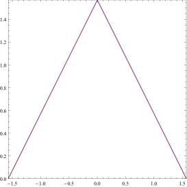
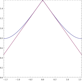
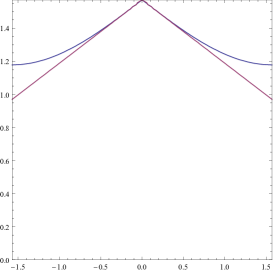
Figure 15: Plots of the boundaries beyond which the space-like geodesic does not exist for $\theta=\frac{\pi}{2}$ (left), $\theta_{0}=\frac{\pi}{4}$ (middle) and $\theta_{0}=\frac{\pi}{8}$ (right). The hoirzontal and vertical coordinates are $\phi$ and $T$ in the range $-\pi/2\leq\phi\leq\pi/2$ and $0\leq T\leq\pi/2$, respectively. We consider the spacelike geodesic which connects two points with $\phi_{1}=-\phi_{2}$ for each time. The blue curves are the boundaries for the dS₃ geodesic length $D_{12}$, while the red ones are those for the dS₂ metric (1.4). Both of which coincide only when $\theta=\frac{\pi}{2}$.

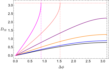
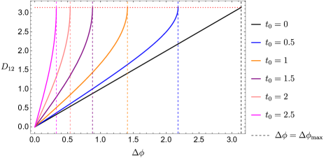
Figure 16: The behaviors of the length $D_{12}$ of space-like geodesics. The left panel shows $D_{12}$ as a function of $|\phi_{1}-\phi_{2}|$ for $\theta_{0}=\frac{\pi}{8}$ at various fixed times $t_{0}$. Notice that at the latter two times, the space-like geodesic ceases to excite for a large values of $\Delta\phi=|\phi_{1}-\phi_{2}|$. The right panel shows $D_{12}$ as a function of $|\phi_{1}-\phi_{2}|$ for the maximal half dS₃i.e., $\theta_{0}=\frac{\pi}{2}$ at fixed times. The horizontal red dotted line describes $D_{12}=\pi$ and vertical dashed lines are referred as the critical size $\Delta\phi_{\mathrm{max}}$.

It is clear that for two different points $\phi_{1}\neq\phi_{2}$, this inequality gets violated at enough later time. On the other hand, if $t_{0}$ and $\theta_{0}$ satisfy

$$\cos(2\theta_{0})\geq 1-\frac{2}{\cosh^{2}t_{0}},$$ (3.7)

then for any values of $\phi_{1}$ and $\phi_{2}$, the space-like geodesic which connects the two points does exist. The geodesic length $D_{12}$ as a function of $\Delta\phi$ at $\theta_{0}=\frac{\pi}{8}$ and $\theta_{0}=\frac{\pi}{2}$ is depicted in figure 16.

When the bound (3.6) is violated, the geodesic length gets complex valued such that its real part is $\pi$:

$$D_{12}=\pi+i\text{arccosh}\left[\sinh^{2}t-\left(\cos^{2}\theta_{0}+\sin^{2}\theta_{0}\cos(\phi_{1}-\phi_{2})\right)\cosh^{2}t_{0}\right].$$ (3.8)

The imaginary contribution comes from the time-like geodesic and the final real part $\pi$ does from the geodesic in an Euclidean space i.e., a semi-sphere (see Hikida:2022ltr ).

Consider the maximal case $\theta_{0}=\frac{\pi}{2}$. In this case, due to the Z₂ symmetry $\theta\to\pi-\theta$, the geodesics which connect two points on the boundary $\theta=\theta_{0}=\frac{\pi}{2}$ are all within the boundary dS₂, as shown in figure 14. At $t_{0}=0$, there is always a geodesic which connects two points on the boundary and the geodesic length is simply found to be

$$D_{12}=\Delta\phi.$$ (3.9)

However for $t_{0}\neq 0$, a space-like geodesic does not exist for $\Delta\phi=|\phi_{1}-\phi_{2}|>\Delta\phi_{\mathrm{max}}$, where the bound is explicitly given by

$$\Delta\phi_{\mathrm{max}}=2\left(\frac{\pi}{2}-\arccos\left(\frac{1}{\cosh t_{0}}\right)\right)=\pi-2\arctan\left[\sinh t_{0}\right]\,.$$ (3.10)

This bound coincides with the boundary of the past light cone of a point at $t=\infty$ and is identical to the condition (2.19) found in our previous analysis of AdS/CFT, shown in the left panel of figure 15. These behaviors of geodesic length are plotted in the right panel of figure 16.

The profile of the geodesic for $\Delta\phi\leq\Delta\phi_{\mathrm{max}}$ is sketched in the left panel of figure 17. When $\Delta\phi>\Delta\phi_{\mathrm{max}}$, the geodesic length gets complex valued and can be interpreted as the union of time-like geodesic and space-like one as depicted in the right panel of figure 17. Note that this transition at $\Delta\phi=\Delta\phi_{\mathrm{max}}$ is peculiar to our dS setup and can not be seen in the AdS setups.

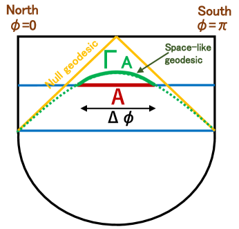
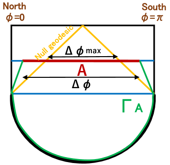
Figure 17: Sketches of connected geodesics $\Gamma_{A}$ in the boundary dS₂ for $\theta=\frac{\pi}{2}$. In the left panel, we present the space-like one with $\Delta\phi\leq\Delta\phi_{\mathrm{max}}$. In the right panel, we plotted what geodesic length computes for $\Delta\phi>\Delta\phi_{\mathrm{max}}$. It is a union of time-like and space-like geodesic.

3.2 Holographic Entanglement Entropy and Violation of Subadditivity

Now let us consider the calculation of the holographic entanglement entropy (1.3) in Case 1 (figure 4), namely Schwinger-Keldysh dS geometry, where there is no EOW brane. In this case, $S_{A}$ for an interval $A$, can be computed from the connected geodesic as

$$S_{A}=\frac{D_{12}}{4G_{N}},$$ (3.11)

whose length was already studied in the previous subsection.

Consider the holographic entanglement entropy at a fixed time $t=t_{0}$ for an interval $A$ defined by $\phi_{1}\leq\phi\leq\phi_{2}$. For a generic choice of the boundary $\theta_{0}$, the holographic entanglement entropy computed as the geodesic length, takes real and positive values only for $\Delta\phi\leq\Delta\phi_{\mathrm{max}}$, as depicted in figure 16. For the maximal value $\Delta\phi=\Delta\phi_{\mathrm{max}}$ we find $D_{12}=\pi$, which is a half of the length of the de Sitter horizon and thus $S_{A}$ becomes a half of de Sitter entropy $S_{A}=\frac{1}{2}S_{\rm dS}$.

In terms of the time evolution, for an earlier time $0\leq t\leq t_{\mathrm{max}}$, $S_{A}$ is well-defined for any value of $\Delta\phi$, where $t_{\mathrm{max}}$ is the time when (3.7) is saturated i.e.

$$t_{\mathrm{max}}=\text{arccosh}\left(\frac{1}{\sin\theta_{0}}\right)=\log\left(\cot\left(\frac{\theta_{0}}{2}\right)\right)\,.$$ (3.12)

However, for $t>t_{\mathrm{max}}$, the behavior of holographic entanglement looks confusing partly because it takes a complex value for $\Delta\phi>\Delta\phi_{\mathrm{max}}$ and also because it is a convex function of $\Delta\phi$ even for $\Delta\phi\leq\Delta\phi_{\mathrm{max}}$ as can be seen from figure 16. The latter fact shows the violation of (strong) subadditivity. Indeed, the second derivative of the geodesic length

$$\frac{d^{2}D_{12}}{d\Delta\phi d\Delta\phi}=\frac{\sqrt{2}\cosh t\sin\theta_{0}\sin\left(\frac{\theta_{0}}{2}\right)\left(\cosh^{2}t\sin^{2}\theta_{0}-1\right)}{\left(1+\cos D_{12}\right)^{3/2}},$$ (3.13)

becomes positive when $t>t_{\mathrm{max}}$. In terms of the conformal time $T$ ($\cosh t\equiv\frac{1}{\cos T}$), the critical time is rewritten as

$$T_{\mathrm{crt}}=\frac{\pi}{2}-\theta_{0}\,,$$ (3.14)

which is nothing but the intersection between the boundary $\theta=\theta_{0}$ and the cosmological horizon located at $T=\frac{\pi}{2}\pm\theta$.

To see why the convex entropy function violates the subadditivity, first note that $S_{A}$ is a function of the length $y=L(A)$ of the interval $A$, owing to the translational invariance. It is obvious from the convex nature $\partial^{2}_{y}S_{A}(y)>0$ that we have $S_{A}(2y)>2S_{A}(y)$, which violates the subadditivity $S_{A}+S_{B}\geq S_{AB}$. Of course, this shows that the strong subadditivity, which is expressed as $S_{AB}+S_{BC}\geq S_{ABC}+S_{B}$, is broken. Refer to figure 18 for plots of the regions where the subadditivity is satisfied, whose further interpretation will be given later. This behavior is a complete contrast to that of AdS/CFT, where the strong subadditivity is always satisfied Headrick:2007km ; Wall:2012uf .

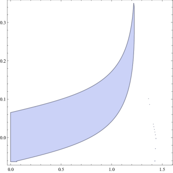
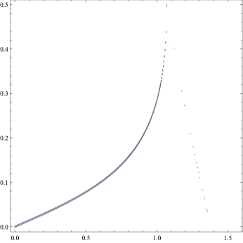
Figure 18: We plotted the behavior of subadditivity violation for $\theta_{0}=\frac{\pi}{4}$ (left) and $\theta_{0}=\frac{\pi}{2}-0.01$ (right). We consider the subsystem $A$ and $B$ such that $A$ connects the two points $(\phi,T)=(0,T_{0})$ and $(1/2,T_{0}+\Delta T)$ and $B$ does the two points $(1/2,T_{0}+\Delta T)$ and $(1,T_{0})$. $T$ is introduced by $\cos T=\frac{1}{\cosh t}$. The horizontal and vertical coordinates describe $T_{0}$ and $\Delta T$. We colored the region where the subadditivity holds i.e. $S_{A}+S_{B}-S_{AB}\geq 0$.

3.3 Static Time Slices

To study the nature of subadditvity violation, let us first focus on the maximal case $\theta_{0}=\frac{\pi}{2}$. In this case, it is useful to consider the static coordinate $(\chi,s)$ of dS₂ introduced as follows

$$\cos\chi=\cos\phi\cosh t,\ \ \ \ \ \cosh s=\frac{\sin\phi}{\sqrt{\frac{1}{\cosh^{2}t}-\cos^{2}\phi}},$$ (3.15)

which leads to the metric

$$ds^{2}=d\chi^{2}-\sin^{2}\chi ds^{2}.$$ (3.16)

Then the geodesic length in the bulk dS₃ which connects between two points $(\chi_{1},s_{0})$ and $(\chi_{2},s_{0})$ on the boundary dS₂ at the same constant time $s_{0}$ is simply given by $D_{12}=|\chi_{1}-\chi_{2}|$. This means that the holographic entanglement entropy on the constant time slice in this static coordinate is linear about the subsystem size $|A|$ and saturates the subadditivity. This clearly shows that if we consider time slices other than $s=$const. , including the constant $t$ slices, the strong subadditivity gets violated because the subsystem size $|A|$ gets shorter as

$$|A|=\int^{\chi_{2}}_{\chi_{1}}d\chi\sqrt{1-\sin^{2}\chi\left(\frac{ds}{d\chi}\right)^{2}}\leq\chi_{2}-\chi_{1}=D_{12}.$$ (3.17)

This analysis shows that at $\theta_{0}=\frac{\pi}{2}$, the static slice $s=$const. is the only time slice which is consistent with the Hilbert space structure of dual unitary quantum systems.

We can provide another feature of this restriction from the spacetime structure of de Sitter space. Consider a Wheeler-DeWitt patch in the bulk dS₃ for a generic time slice of the boundary dS₂. Since space-like geodesics which connects two boundary points are all on the boundary dS₂, the geodesics are outside of the Wheeler-DeWitt patch, except when the time slice is the constant $s$ slice, as depicted in figure 19 by comparing this with that in AdS. In a sensible holography we expect that any bulk counterpart dual to objects in the boundary theory at a specific time will be within its Wheeler-DeWitt patch.

For generic values of $\theta_{0}$, the situation gets less sharp but looks qualitatively similar. This can be seen from the left panel of figure 18. As the time evolves following constant $t$ (or equally $T$) slices, the region which satisfies the subadditivity gets squeezed into the future direction and eventually disappears. As $\theta_{0}$ gets closer to $\frac{\pi}{2}$, the region which satisfies the subadditivity becomes very narrow as in the right panel of figure 18.

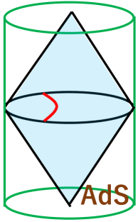
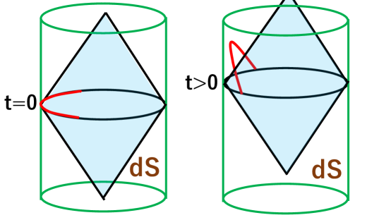
Figure 19: Sketches of Wheeler-DeWitt patches (blue regions) and the geodesics (red curves) in AdS₃ (left), in dS₃ at $t=0$ (middle) and in dS₃ at $t>0$ (right).

3.4 Time slices and dual Hilbert space

Having in mind the analysis of holographic entanglement entropy, we would like to consider the holographic dual interpretation. For simplicity let us focus on the case $\theta_{0}=\frac{\pi}{2}$. From the Hilbert space viewpoint of its dual quantum system, assuming that it is unitary, we can only allow the static time slice (constant $s$ one) on the boundary dS₂ as we have seen in the previous subsection. Owing to the $SO(2,1)$ symmetry of dS₂, we can boost and rotate the canonical static time slice $t=0$ by this symmetry as depicted in the left panel of figure 20. Below we call these $SO(2,1)$ transformation of $t=0$ slice nice slices. Note that this family of nice time slices do not include $t=t_{0}>0$ slices but does the constant $s$ ones in the coordinate (3.16). Therefore we expect that all nice slices correspond to an identical Hilbert space ${\cal H}_{\mathrm{dS}}$ of a quantum system dual to a half dS₃. Since the dual state looks maximally entangled due to the fact that the extremal surface $\Gamma_{A}$ is included in the boundary dS₂, the dimension of ${\cal H}_{\mathrm{dS}}$ should be given by $S_{dS}=\frac{2\pi}{4G_{N}}$, i.e. the de Sitter entropy of the dS₃ gravity.

This argument looks very similar to the surface/state duality proposed in Miyaji:2015yva , which argues that a codimension two space-like surface $\Sigma$ in general gravitational spacetimes is holographically dual to a certain quantum state $|\Phi_{\Sigma}\rangle$. The difference is that in the present paper we put a real boundary by restricting the dS₃ to the half dS₃ so that it has a genuine boundary given by dS₂ at $\theta=\theta_{0}$. However, it is natural that there is a holographic duality even before we put the time-like boundary. In this context, our lesson from this present analysis is that in order for the surface/state duality works well we need to require that the extemal surface $\Gamma_{A}$ should be within the Wheeler-DeWitt patch of $\Sigma$.

We can decompose a constant $t=t_{0}>0$ slice into multiple nice time slices as depicted in the right panel of figure 20. As $t_{0}$ gets larger, we need more nice time slices to cover it as can be seen from that fact that the length of $t=t_{0}$ slice exponentially grows $\sim e^{t_{0}}$. This shows that the constant $t$ slice (except $t=0$ one) overestimates the dimension of Hilbert space. Indeed this is obvious from the fact that to cover the $t=t_{0}$ slice we need many nice slices whose Hilbert spaces clearly have overlaps as they cover the $t=0$ slice many times. Thus we cannot expect that such a slice describes a well-defined Hilbert space, which is consistent with our observation of the subadditivity violation. The division of the constant $t$ slice into subsystems does not correspond to the factorization of a Hilbert space. This behavior is quite different from that in local quantum field theories, where the choice of time slice on a given causal diamond gives the identical subsystem of a Hilbert space. In our de Sitter holography, even though the segment $A$ on the constant $t$ slice and $\Gamma_{A}$ on the nice slice both live on the same causal diamond as in the left panel of figure 17, only the latter has a well-defined meaning as a proper subsystem of ${\cal H}_{\mathrm{dS}}$.

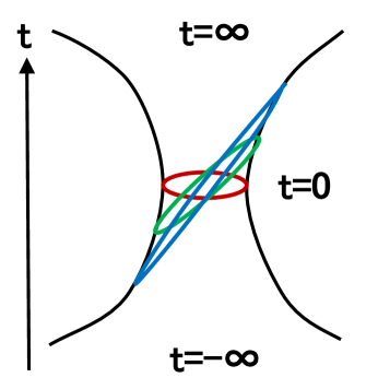
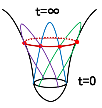
Figure 20: Sketches of nice time slices (constant $s$ slices) in the boundary dS₂ which describe the Hilbert space of dual quantum system. In the left panel we showed these slices in a global dS₂. In the right panel, we showed that a constant $t$ slice (red curve) is decomposed into multiple constant $s$ slices (purple, blue and green curves).

3.5 Non-locality and Holographic Entanglement Entropy

Then it is natural to ask why only nice slices (constant $s$ slices) can describe a proper Hilbert space. Even though we do not give a conclusive answer to this question, we would like to suggest that the non-local nature of dual quantum system plays a crucial role. First of all, it is obvious that the way we put the boundary of a half dS₃ leads to a finite cut off in the dual field theory. Also the volume law entanglement which we observe for nice slices is typical for vacuum states in highly non-local field theories Li:2010dr ; Shiba:2013jja . Moreover, we can even find that a growth of entanglement entropy, defined by the replica method, can exceed the volume law i.e. $S_{A}\sim|A|^{p},\ \ p>1$ in highly non-local field theories, which shows the violation of subadditivity. Indeed, as shown in Li:2010dr via the replica method, a non-local free scalar field theory in $d$ dimensions with the action

$$S=\int dx^{d}\phi(x)e^{(-\partial_{x}^{2})^{q}}\phi(x)\,,$$ (3.18)

leads to the entanglement entropy whose UV divergence scales as

$$S_{A}\propto\left(\frac{L_{A}}{\epsilon}\right)^{d-2+2q}\,,$$ (3.19)

where $L_{A}$ is the linear size of the subsystem $A$. Thus, $S_{A}$ grows faster than the volume law if $q>\frac{1}{2}$. Here note that the entanglement entropy defined from the replica method based on Euclidean path-integral is not guaranteed to satisfy the subadditivity, though the entanglement entropy defined from a quantum state in a Hilbert space automatically satisfies the subadditivity.

In our holographic dual of a half dS₃, it is natural to expect that a similar non-local field appears and this may explain the violation of subadditivity on generic time slices. As the value of $\theta_{0}$ gets smaller, this non-local effects get milder and the range of time slices which satisfy the subadditivity, gets broader as depicted in figure 18.

In this way, even though the proper Hilbert space interpretation becomes difficult for generic time slices including constant $t$ slices, we may be able to formally define the entanglement entropy by the replica method, which allows the violation of strong subadditivity. Notice that in such a non-local field theory, Hamiltonian cannot be defined in a standard way as the action involves derivatives with respect to the Euclidean time whose order is higher than two. If this interpretation is true, we should be able to define $S_{A}$ even when $A$ is so large that the two end points of $A$ cannot be connected by a space-like geodesic. If we apply the original holographic entanglement entropy formula (3.11), we find that it is complex valued

$$D_{12}=\pi+i\text{arccosh}\left[\sinh^{2}t-\cos(2\theta_{0})\cosh^{2}t_{0}\right]\,.$$ (3.20)

See Hikida:2022ltr ; Chapman:2022mqd for more studies about complex geodesics in dS space. As depicted in the right panel of figure 17, the real part comes from the geodesic in the Euclidean instanton (semi-sphere) and the imaginary part comes from the time-like geodesic in the de Sitter space. However, if we consider the holographic calculation of entanglement entropy via the replica method (for the derivation of the covariant HEE in AdS/CFT see Dong:2016hjy ), there are two candidates of extremal surface: one is in the bra geometry and the other is the ket geometry as in figure 21. This prescription was analyzed in Chen:2020tes for a bra-ket wormhole in AdS/CFT.

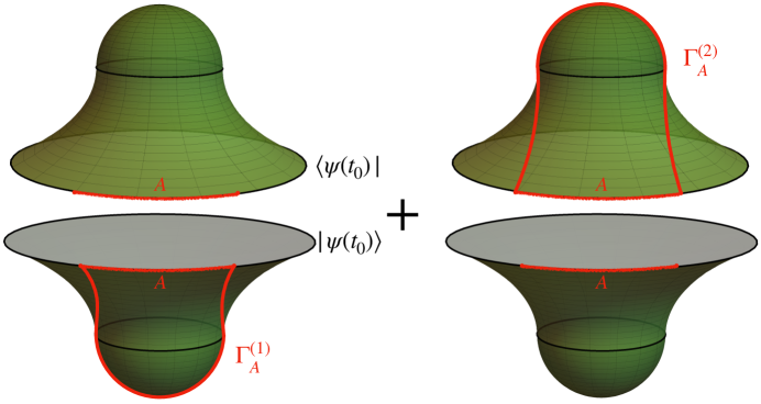
Figure 21: Sketches of calculation of holographic entanglement entropy in the Schwinger-Keldysh geometry. The sum of the contributions associated with two extremal surfaces $\Gamma^{(1)}_{A},\Gamma^{(2)}_{A}$ gives rise to the real entanglement entropy.

The correct result is given by the sum of two contributions:

$$Z^{(n)}_{\mathrm{tot}}=e^{(1-n)S}+e^{(1-n)S^{*}},$$ (3.21)

where $n$ is the replica number. $S_{A}$ is given by

$$S_{A}=\lim_{n\to 1}\frac{1}{1-n}\log Z^{(n)}_{\mathrm{tot}}\simeq\frac{S+S^{*}}{2}=\mbox{Re}[S].$$ (3.22)

Thus we find that the actual $S_{A}$ is given by the real part:

$$S_{A}=\frac{\pi}{4G_{N}}=\frac{1}{2}S_{\mathrm{dS}},$$ (3.23)

where $S_{\mathrm{dS}}=\frac{2\pi}{4G_{N}}$ is the de Sitter entropy.

In this way, we find that the saturation behavior i.e. $S_{A}$ grows monotonically for $0\leq\Delta\phi\leq\Delta\phi_{\mathrm{max}}$ and it takes the constant value $\frac{1}{2}S_{\mathrm{dS}}$ for $\Delta\phi\geq\Delta\phi_{\mathrm{max}}$. For $\Delta\phi>\pi$, the standard holographic prescription guarantees the relation $S_{A}=S_{A^{c}}$, where $A^{c}$ is the complement of $A$. Explicit plots are shown in figure 22.

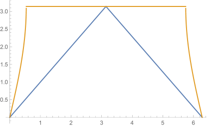
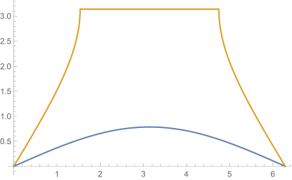
Figure 22: Plots of holographic entanglement entropy $S_{A}$ on a constant $t$ time slice based on the prescription (3.22) for $d=2$. We plotted $S_{A}$ as a function of $\Delta\phi$ in the range $0\leq\Delta\phi\leq 2\pi$ for $\theta_{0}=\frac{\pi}{2}$ (left) and $\theta_{0}=\frac{\pi}{8}$ (right). The blue and orange curves correspond to $t=0$ and $t=2$. Note that we have the critical time $t_{\mathrm{max}}=0$ for $\theta_{0}=\frac{\pi}{2}$ and $t_{\mathrm{max}}\simeq 1.61$ for $\theta_{0}=\frac{\pi}{8}$.

3.6 Overcounting of de Sitter Hilbert Space

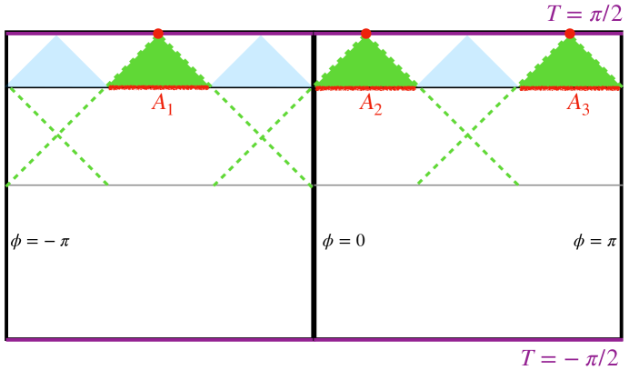
Figure 23: Penrose diagram of dS₂ spacetime which corresponds to the dS boundary located at $\theta=\theta_{0}=\frac{\pi}{2}$ in dS₃ bulk spacetime. The green dashed lines denote the null limit of geodesics. On the time slice $T=T_{0}$ or $t=t_{0}$, we divide the system into six parts.

In previous analyses regarding the holographic entanglement entropy of a single interval, it was observed that the entropy is bounded by half of the dS entropy, i.e.,

$$S_{A}\leq\frac{1}{2}S_{\mathrm{dS}}\,,$$ (3.24)

as illustrated in figure 22. This outcome is expected since the corresponding bulk dual represents only half of the dS spacetime. Generalizing this calculation to cases where subsystem $A$ comprises multiple disconnected intervals is also possible. Since this calculation follows the standard prescription Headrick:2010zt , explicit results will not be presented in detail. However, it is important to note that the holographic entanglement entropy of a subregion consisting of multiple intervals is not bounded by the dS entropy $S_{\rm dS}$ at late times, as the sum of lengths of disconnected geodesics can be very large. Focusing on the case with the boundary dS space located at $\theta=\theta_{0}=\frac{\pi}{2}$, it has been derived in eq. (A.4) that the entropy of a single interval reaches the maximal value $\frac{1}{2}S_{\mathrm{dS}}$ when its length corresponds to the critical size $\Delta\phi_{\rm max}$. It should be noted that the maximum size $\Delta\phi_{\rm max}(t_{0})$ decreases to zero as the boundary time $t_{0}$ increases. Consequently, let us consider a time slice at $t=t_{0}$ which can be divided into $2N$ identical intervals, where $\frac{\pi}{N}\geq\Delta\phi_{\rm max}(t_{0})$. Figure 23 provides an explicit example with $N=3$. By considering a subsystem with $N$ intervals, one can find that the holographic entanglement entropy is shown as

$$S_{A_{1}\cup A_{2}\cup\cdots\cup A_{N}}=N\times S_{A_{i}}=\frac{N}{2}S_{\rm dS}\geq S_{\rm dS}\,.$$ (3.25)

This value can even approach infinity as $N$ tends to infinity, while $\lim\limits_{t_{0}\to\infty}\Delta\phi_{\rm max}\to 0$. It might be questioned whether this violates the entropy bound of de Sitter space, whose Hilbert space is expected to be finite. However, as observed from the violation of (strong) subadditivity, we expect that a generic time slice does not correspond to a pure state in a single de Sitter Hilbert space. Instead, the unbounded entropy of multiple intervals, as expressed in eq. (3.25), can be interpreted as the result of overcounting the dimension of the de Sitter Hilbert space. As shown in figure 23, each critical interval $A_{i}$ at $t=t_{0}$ could be understood as a maximally entangled state in a single de Sitter Hilbert space. Back to the original time at $t=0$, those single Hilbert spaces are overlapping with each other along this time slice. The recent paper Cao:2023gkw discusses the tensor network representation of dS space with overlapping qubits. However, we note that the studies in Cao:2023gkw focus on bulk dS spacetime which is different from our dS boundary picture as shown in figure 23.

3.7 Higher dimensional half de Sitter space

It is straightforward to generalize our analysis for a half dS₃ to a half dS_d+1 for $d\geq 3$. Below we will provide analysis for $\theta_{0}=\frac{\pi}{2}$ in the global dS_d+1 described by (1.1) and (1.2). The time-like boundary of this space is given by dS_d described by the global metric

$$ds^{2}=-dt^{2}+\cosh^{2}t(d\phi^{2}+\sin^{2}\phi d\Omega^{2}_{d-2}),$$ (3.26)

where $d\Omega^{2}_{d-1}$ is the metric of the unit sphere S^d-2. As in the previous case of $d=2$, we would like to argue that gravity on a half dS_d+1 is dual to non-local field theory on the dS_d.

To examine this duality we would like to calculate the holographic entanglement entropy. This is given by the area of extremal surface $\Gamma_{A}$, which ends on the boundary of the subsystem $A$, by (1.3).

For this we choose the subsystem $A$ to be a disk on the boundary dS_d:

$$t=t_{0},\ \ 0\leq\phi\leq\phi_{1}.$$ (3.27)

In this case, we can find the profile of the extremal surface $\Gamma_{A}$ which ends on the boundary $\phi=\phi_{1}$ of the subsystem $A$ (3.27) as

$$\frac{\cos\phi}{\tanh t}=\frac{1+L^{2}}{1-L^{2}}.$$ (3.28)

This surface can be simply obtained by mapping the extremal surface

$$t^{2}-\sum_{i=1}^{d-1}(x_{i})^{2}=L^{2},$$ (3.29)

in the Poincare dS_d given by the metric

$$ds^{2}=\frac{-dt^{2}+\Sigma_{i=1}^{d-1}dx_{i}^{2}}{t^{2}}.$$ (3.30)

The constant $L$ is related to the choice of the subsystem $A$ via

$$\frac{1+L^{2}}{1-L^{2}}=\frac{\cos\phi_{1}}{\tanh t_{0}}.$$ (3.31)

The profile of the extreme surface (3.28) is plotted in figure 24.

This $d-1$ dimensional extremal surface $\Gamma_{A}$ is wrapped on S^d-2. The induced metric on $\Gamma_{A}$ reads

$$ds^{2}=\frac{4L^{2}(1+L^{2})^{2}}{\left((1+L^{2})^{2}-(1-L^{2})^{2}\cos^{2}\phi\right)^{2}}d\phi^{2}+\frac{(1+L^{2})^{2}\sin^{2}\phi}{(1+L^{2})^{2}-(1-L^{2})^{2}\cos^{2}\phi}d\Omega^{2}_{d-2}.$$

This surface $\Gamma_{A}$ is space-like when $0<L^{2}\leq 1$. It becomes light-like when $L^{2}=0$ and time-like when $L^{2}<0$.

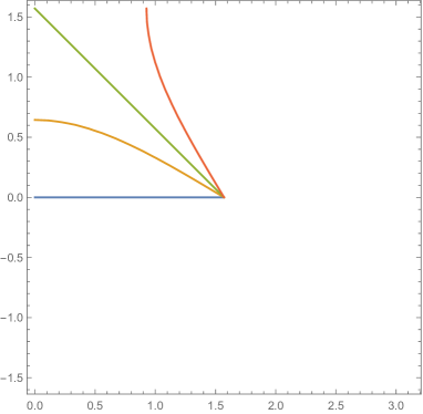
Figure 24: Profiles of extremal surfaces (3.28) in global dS. The horizontal and vertical coordinate are $\phi$ and $T$, respectively. The blue, yellow, green ,and red curves describe the extremal surface for $L^{2}=1,1/4,0$ and $-1/4$, respectively.

The area of $\Gamma_{A}$ is computed as

$$A(\Gamma_{A})=\mathrm{Vol}(\mathrm{S}^{d-2})\int^{\phi_{1}}_{0}d\phi\frac{2L(1+L^{2})^{d-1}(\sin\phi)^{d-2}}{\left((1+L^{2})^{2}-(1-L^{2})^{2}\cos^{2}\phi\right)^{\frac{d}{2}}}.$$ (3.33)

Since this is a function of $\phi_{1}$ and $t_{0}$, we write this as $A(\phi_{1},t_{0})$. It is straightforward to see that at $t_{0}=0$ and $\phi_{1}=\frac{\pi}{2}$ we have

$$A\left(\frac{\pi}{2},0\right)=\frac{1}{2}\mbox{Vol}(S^{d-1}).$$ (3.34)

This means that the corresponding holographic entanglement entropy coincides with the half of de Sitter entropy $\frac{1}{2}S_{dS}$. The behavior of $A(\phi_{1},t_{0})$ is plotted in figure 25. In general it is a monotonically increasing function of $t_{0}$ and $\phi_{1}$ and gets finally saturated to the maximal value $\frac{1}{2}S_{dS}$. Note that when $L^{2}$ becomes negative i.e when $\Gamma_{A}$ gets time-like, we choose the other extremal surface which goes past and which is wrapped on the semi-sphere in the Euclidean part as in right panel of figure17. Thus as in the same argument of (3.23), the holographic entanglement entropy is given by the real part of $A(\Gamma_{A})$, namely $\frac{1}{2}S_{\rm dS}$.

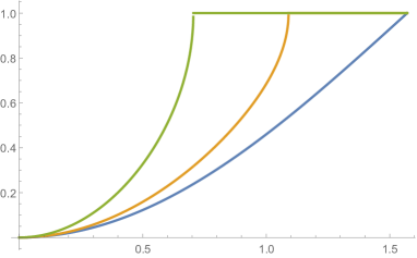
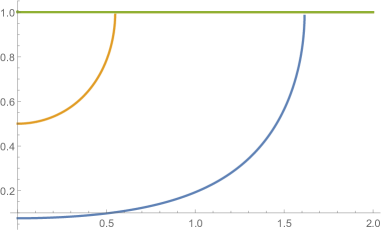
Figure 25: The behaviors of the holographic entanglement entropy for a half dS₄ ($d=3$) in case 1. In the left panel, we plotted $\frac{1}{2\pi}A(\Gamma_{A})$ as a function of $\phi_{1}$ at $t=0$ (blue), $t=1/2$ (orange) and $t=1$ (green). In the right panel, we showed $\frac{1}{2\pi}A(\phi_{1},t_{0})$ as a function of $t_{0}$ for $\phi_{1}=\pi/8$ (blue), $\phi_{1}=\pi/3$ (orange), $\phi_{1}=\pi/2$ (green).

4 Holography for a half dS with EOW brane (Case 2)

Now we would like to study another setup of holography for a half de Sitter space in the presence of EOW brane (case 2). We regard the future boundary $t=\infty$ of the de Sitter space as an EOW brane where we impose the Neumann boundary condition for the gravitational field. In the dual field theory, we have the final state projection as in the case of AdS/CFT analysis done in section 2.3.

To obtain the properties of the gravity dual, we would like to analyze the holographic entanglement entropy given by the area of extremal surface as in (1.3) and (3.11). However, since the field theory sides has the final state projection, it should properly be regarded as the holographic pseudo entropy Nakata:2021ubr . For simplicity focus on the maximal case $\theta_{0}=\frac{\pi}{2}$ in dS_d+1 for simplicity. We argue gravity in the half dS_d+1 with the EOW brane at $t=t_{P}$ is dual to a non-local field theory on its boundary dS_d with a finial state projection at $t=t_{p}$. The new aspect here is that the space-like extremal surface can end on the boundary of the EOW brane.

Consider the case where the EOW brane is situated at the future infinity $t_{p}\to\infty$, which is dual to the final state projection at the future infinity.

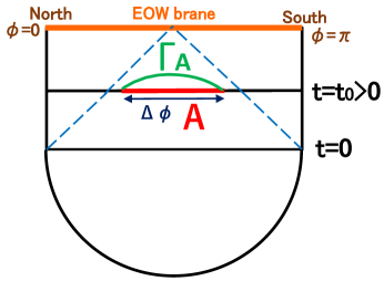
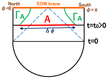
Figure 26: Sketches of geodesics in dS₂ which are used to calculation the holographic pseudo entropy in a half dS₃. When the subsystem $A$ is small $\Delta\phi\leq\Delta\phi_{\mathrm{max}}$, the geodesic $\Gamma_{A}$ is space-like and connected shown in the left panel. On the other hand when $A$ gets larger $\Delta\phi>\Delta\phi_{\mathrm{max}}$, $\Gamma_{A}$ consists of two disconnected time-like geodesics as in the right panel.

First let us analyze the holographic pseudo entropy in this setup for $d=2$. When the interval $A$ is small such that $\Delta\phi<\Delta\phi_{\mathrm{max}}$, the holographic pseudo entropy $S_{A}$ is given by the length of connected space-like geodesic $D^{\mathrm{con}}_{12}$ as we had in the case 1. However, for $\Delta\phi>\Delta\phi_{\mathrm{max}}$, when a connected space-like geodesic does not exist, $S_{A}$ can be computed from the two disconnected geodesics which connect one of the end points of $A$ with a point on the EOW brane as depicted in figure 26.

Note also that such a disconnected geodesic becomes time-like for $\Delta\phi>\Delta\phi_{\mathrm{max}}$, which shows that the holographic pseudo entropy is pure imaginary. This is the crucial difference from the analysis of $S_{A}$ in the case 1. In the case 2, in the presence of EOW brane, the geodesics $\Gamma_{A}$ can end on it and the real part of $S_{A}$ for this contribution (see the right panel of figure 26) becomes smaller than the connected one (see the right panel of figure 17) which has a positive real part.

In summary, the behavior of $S_{A}$ for $d=2$ is identical to that in section 3.5 for $\Delta\phi<\Delta\phi_{\mathrm{max}}$, while we have $\mathrm{Re}[S_{A}]=0$ for $\Delta\phi>\Delta\phi_{\mathrm{max}}$:

$$\mbox{For}\ 0\leq\Delta\phi<\Delta\phi_{\mathrm{max}}:\ \ \ \ S_{A}=\frac{D^{\mathrm{con}}_{12}}{4G_{N}},$$

$$\mbox{For }\Delta\phi>\Delta\phi_{\mathrm{max}}:\ \ \ \ \mbox{Re}[S_{A}]=0.$$ (4.1)

It is straightforward to generalize this to higher dimensions by employing the results of $A(\phi_{1},t_{0})$ in case 1 presented in section 3.7. When $\phi_{1}$ is smaller than the saturation value in case 1, $S_{A}$ takes the same value as that in case 1. For large values of $\phi_{1}$, we have Re$[S_{A}]=0$. An explicit plot for $d=3$ is shown in figure 27.

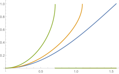
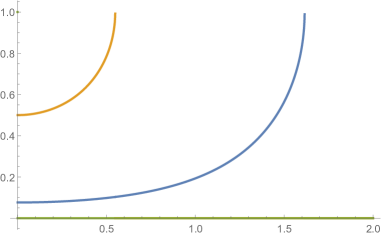
Figure 27: The behaviors of the holographic pseudo entropy for a half dS₄ ($d=3$) in case 2. In the left panel, we plotted $\frac{1}{2\pi}A(\Gamma_{A})$ as a function of $\phi_{1}$ at $t=0$ (blue), $t=1/2$ (orange) and $t=1$ (green). In the right panel, we showed $\frac{1}{2\pi}A(\Gamma_{A})$ as a function of $t_{0}$ for $\phi_{1}=\pi/8$ (blue), $\phi_{1}=\pi/3$ (orange), $\phi_{1}=\pi/2$ (green).

Now let us interpret the behavior of $S_{A}$ in terms of dual field theory on dS_d. For $\Delta\phi<\Delta\phi_{\mathrm{max}}$, $S_{A}$ is identical to that in case 1, its interpretation is the same. Thus, we find the violation of subadditivity and this is expected to be due to the non-local nature of the dual field theory. For $\Delta\phi>\Delta\phi_{\mathrm{max}}$, we find a behavior special to case 2 that the real part of $S_{A}$ does vanish.

This transition at $\Delta\phi=\Delta\phi_{\mathrm{max}}$ may be natural from the viewpoint of the dual field theory on dS_d. To see this, let us remember that the pseudo entropy is defined from the transition matrix (1.5), which depends on the two states $|\psi_{1}\rangle$ and $|\psi_{2}\rangle$. In our setup $|\psi_{1}\rangle$ is the state which is obtained by the forward time evolution of Hartle-Hawking state, while $|\psi_{2}\rangle$ is the one created by the backward time evolution of the final state. It is also useful to note that the phenomenological observation Mollabashi:2020yie ; Mollabashi:2021xsd ; Akal:2021dqt implies that the real part of pseudo entropy typically measures the amount of entanglement in the intermediate state between the two states, though the interpretation of imaginary part is not well understood at present. Now the final state is defined by imposing a boundary condition at $t=t_{p}=\infty$ and the analysis of the space-like EOW brane Akal:2020wfl suggests that the state has no real space entanglement as in the standard boundary state Miyaji:2014mca . At the time slice $t=t_{0}$, we can have such an disentangling effect from a point at future infinity when two points are separated more than $2(t_{p}-t_{0})$ assuming the light like propagation of physical signals on dS_d. Indeed this border is $\Delta\phi_{\mathrm{max}}$. Therefore it is natural that the real part of pseudo entropy gets vanishing for $\Delta\phi>\Delta\phi_{\mathrm{max}}$. On the other hand, for $\Delta\phi<\Delta\phi_{\mathrm{max}}$, such two points do not feel the existence of the EOW brane and thus the result is the same as that in case 1.

In a similar way, we can analyze the holographic pseudo entropy when the final projection is inserted at a finite time $t=t_{p}$. Obviously at $t=t_{p}$, we have $S_{A}=0$. Moreover, the real part of $S_{A}$ gets vanishing when the geodesic $\Gamma_{A}$ becomes light-like. This can happen $t<t_{p}$ if the subsystem $A$ is large enough, in which case a imaginary part of $S_{A}$ starts to be non-zero until $t=t_{p}$ as $\Gamma_{A}$ becomes time-like, as depicted in figure 28 for plots. It is curious to note that this page curve like behavior of Re$S_{A}$ is qualitatively similar to the one found for the AdS/CFT setup in eq. (2.33).

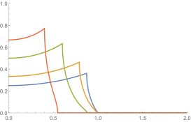
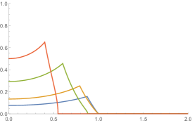
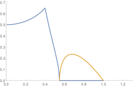
Figure 28: The behaviors of the holographic pseudo entropy for a half dS₃ ($d=2$, left) and a half dS₄ ($d=3$, middle and right) in case 2 with the EOW brane at $t_{p}=1$. We plotted $\frac{1}{\pi}A(\Gamma_{A})$ (for $d=2$, left) and $\frac{1}{2\pi}A(\Gamma_{A})$ (for $d=3$, middle) as a function of time $t_{0}$. We chose $\phi_{1}=\frac{\pi}{8}$ (blue), $\phi_{1}=\frac{\pi}{6}$ (orange), $\phi_{1}=\frac{\pi}{4}$ (green), $\phi_{1}=\frac{\pi}{3}$ (red). In the right panel, we plotted Re$\left[\frac{1}{2\pi}A(\Gamma_{A})\right]$ (blue) and Im$\left[\frac{1}{2\pi}A(\Gamma_{A})\right]$ (orange) as a function of time for $\phi_{1}=\frac{\pi}{3}$ for $d=3$. Note that the real part starts vanishing when the geodesic becomes null and we have both the real and imaginary part vanishing for $t>t_{p}(=1)$.

5 Summary and Discussions

The primary objective of this paper is to investigate the holographic duality involving gravity in de Sitter spaces. Unlike many other approaches, our focus centers on a half de Sitter space, achieved by introducing a timelike boundary in global dS spacetime. Within this framework, we propose that the gravity on a $d+1$-dimensional half de Sitter space is dual to a non-local field theory residing on its $d$-dimensional boundary.

Before delving into our investigation of de Sitter holography, we conducted an analysis of the holographic duality linking gravity in a $d+1$-dimensional AdS and a CFT living on a $d$-dimensional dS. This particular scenario can be regarded as a special case within the framework of the AdS/CFT correspondence. Of course, its validity and fundamental computational methods are well-established. We examined two distinct setups, referred to as the Case 1 and the Case 2, respectively. In the Case 1, the quantum state in the dual CFT is described by the Schwinger-Keldysh formalism, whereas in the Case 2, we consider the dual CFT incorporating a final state projection, as illustrated in figure 4 and figure 5. In particular, the gravity dual in the Case 2 is given by adding an end-of-the-world brane (EOW brane) on an AdS geometry.

In these setups, we evaluated holographic entanglement entropy, which is determined by the area of an extremal surface. In the Case 1, we observed that the holographic entanglement entropy for a subsystem of fixed size consistently increases as the size of de Sitter space is inflating with respect to the global time. Conversely, in the Case 2, it initially presents growth but eventually decreases to zero. At the time $t=t_{\textrm{\tiny P}}$, corresponding to the implementation of the final state projection, the entanglement entropy vanishes. It is important to note that the extremal surface area we computed should be more appropriately interpreted as the pseudo entropy due to the presence of the final state projection. Additionally, we also confirmed that independent CFT calculations in CFT₂ reproduce the results which agree with that from gravity dual.

With the AdS/CFT results as our foundation, we proceeded to examine holography for gravity in a half de Sitter space. We focused on two setups, namely the Case 1 and the Case 2, and investigated the behaviour of holographic entanglement entropy. Note that we employed the standard calculation of holographic entanglement entropy Ryu:2006bv ; Ryu:2006ef ; Hubeny:2007xt , where we minimize the area, as opposed to the prescription in Susskind:2021esx where the area is maximized. Remarkably, we discovered that the properties of holographic entanglement entropy in a half de Sitter space diverge from those in the AdS/CFT correspondence. Notably, connecting two arbitrary points in a global de Sitter space using a spacelike geodesic is not always possible. Consequently, for a two-dimensional dS space, which serves as the timelike boundary of a three-dimensional half de Sitter space, there is typically no spacelike geodesic linking the endpoints of an interval. As a result, the definition of holographic entanglement entropy, denoted as $S_{A}$, in a conventional sense is problematic. Similarly, we observed the same limitation for extremal surfaces in higher dimensions ($d>2$).

However, a resolution to this issue arises when we consider both timelike and spacelike geodesics within a Hartle-Hawking contour, as illustrated in the right panel of figure 17. The joint geodesics allow us to connect two endpoints beyond critical size. Consequently, the holographic entanglement entropy, denoted as $S_{A}$, acquires a complex value. In the Case 1, we contend that the appropriate holographic entanglement entropy can be obtained by taking its real part, which is nothing but half of the de Sitter entropy $\frac{1}{2}S_{dS}$. In the Case 2, with the presence of the EOW brane, we argue that the holographic pseudo entropy can be computed by utilizing timelike geodesics terminating on the EOW brane, as depicted in the right panel of figure 26.

Furthermore, even within parameter regions where a spacelike geodesic exists, the holographic entanglement entropy generally exhibits super-extensive behaviour relative to the subsystem size. Consequently, the corresponding function describing holographic entanglement entropy violates the (strong) subadditivity property. Notably, we have discovered that this issue is resolved solely by focusing on the time slices associated with the static coordinate in the case of the maximal half de Sitter space ($\theta_{0}=\frac{\pi}{2}$). On these particular time slices, the holographic entanglement entropy $S_{A}$ adheres to the volume law. In this regard, we anticipate that the quantum state represented by the half de Sitter space manifests maximal entanglement specifically on these special time slices. This implies that we can establish a well-defined Hilbert space solely for static time slices. Conversely, a generic time slice in the boundary de Sitter space spans the same Hilbert space as the static time slice multiple times, resulting in an overcounting of the genuine degrees of freedom (refer to figure 20). Additionally, it is worth noting that when subadditivity is violated, the extremal surface extends beyond the Wheeler-DeWitt patch, as depicted in figure 19.

Although providing a Hilbert space interpretation for generic time slices, including the constant time slice of the global coordinate, presents challenges, we propose a potential understanding of the entanglement entropy by employing the replica method and defining the area of extremal surface $S_{A}$ as the entropy. Notably, in highly non-local field theories, the realization of super-extensive entanglement entropy can be realized. It is important to note that in such non-local field theories, a standard Hilbert space cannot be defined due to the appearance of infinitely many time derivatives in the action. Applying this perspective, the holographic entanglement entropy in the Case 1 exhibits initial growth, followed by saturation at $\frac{1}{2}S_{dS}$, as depicted in figure 22 and figure 25. Note that this saturation was absent in the evolution of $S_{A}$ derived in the Case 1 in the framework of the AdS/CFT correspondence and that it shows that the entropy is bounded in de Sitter space.

In the Case 2, we observe that the real part of the holographic pseudo entropy exhibits initial growth and eventually vanishes at the critical time, while the imaginary part remains non-zero, as depicted in figure 27 and figure 28. We identify that the real part of $S_{A}$ becomes zero when the subsystem $A$ surpasses the light cone (refer to the right panel of figure 26). This behaviour arises due to the influence of the EOW brane, where the reflection of two points on $A$ by the EOW brane boundary condition affects $S_{A}$. The EOW brane boundary state possesses vanishing quantum entanglement, thereby diminishing the overall quantum entanglement.

There are several promising avenues for future investigation. Firstly, it would be intriguing to explore alternative frameworks that provide a more manageable description of the “overcounting” phenomenon in the Hilbert space dual to a half de Sitter space in global coordinates. One possible approach could involve qubit systems or tensor networks, offering a more controllable perspective. Additionally, it is of great interest to extend our analysis to holography in more generic asymptotically dS spacetimes, such as de Sitter black holes, as well as various cosmological models. Lastly, a pivotal and profound question lies in understanding how the creation and evolution of the universe can be described in terms of the dual field theory, utilizing the insights gained from the holographic duality.

Appendix A Explicit Space-like Geodesics in dS₃

Here we study the connected geodesic anchored on the boundaries of an interval $A$ in dS₃. This is the geodesic which connects $(t,\theta,\phi)=(t_{0},\frac{\pi}{2},-\phi_{0}+\frac{\pi}{2})$ and $(t,\theta,\phi)=(t_{0},\frac{\pi}{2},\phi_{0}+\frac{\pi}{2})$ in the coordinate of dS₃ (3.2). We assume $t_{0}\geq 0$ without losing generality. The length $L$ of a curve is

$$L=\int^{\phi_{0}+\frac{\pi}{2}}_{-\phi_{0}+\frac{\pi}{2}}d\phi\sqrt{\cosh^{2}t-\left(\frac{dt}{d\phi}\right)^{2}}.$$ (A.1)

This leads to the differential equation

$$\frac{dt}{d\phi}=\cosh t\sqrt{1-\frac{\cosh^{2}t}{\cosh^{2}t_{*}}},$$ (A.2)

where the middle point $\phi=\frac{\pi}{2}$ is the turning point and we set $t=t_{*}$ at this point. By integrating this, we find

$$\phi_{0}=\frac{\pi}{2}-\arctan\left[\frac{\cosh t_{*}\sinh t_{0}}{\sqrt{\cosh^{2}t_{*}-\cosh^{2}t_{0}}}\right],$$

$$L=\pi-2\arctan\left[\frac{\sinh t_{0}}{\sqrt{\cosh^{2}t_{*}-\cosh^{2}t_{0}}}\right].$$ (A.3)

Note that assuming $t_{0}>0$, there is an upper bound of $\phi_{0}$, reached at $t_{*}\to\infty$, which we call $\phi_{\max}$:

$$\phi_{\mathrm{max}}=\frac{\pi}{2}-\arctan\left[\sinh t_{0}\right].$$ (A.4)

In this maximal case, we find $L|_{\phi=\phi_{*}}=\pi$, which is a half of de Sitter horizon length. This maximal value $\phi=\phi_{\mathrm{max}}$ corresponds to the limit where the original space-like geodesic gets light-like as depicted in the left panel of figure 17. Therefore we cannot find an appropriate space-like geodesic when the subsystem $A$ is larger than this maximal size.

References

- (1) G. ’t Hooft, Dimensional reduction in quantum gravity, Conf. Proc. C 930308 (1993) 284 [gr-qc/9310026].
- (2) L. Susskind, The World as a hologram, J. Math. Phys. 36 (1995) 6377 [hep-th/9409089].
- (3) J. M. Maldacena, The Large N limit of superconformal field theories and supergravity, Adv. Theor. Math. Phys. 2 (1998) 231 [hep-th/9711200].
- (4) S. S. Gubser, I. R. Klebanov and A. M. Polyakov, Gauge theory correlators from noncritical string theory, Phys. Lett. B 428 (1998) 105 [hep-th/9802109].
- (5) E. Witten, Anti-de Sitter space and holography, Adv. Theor. Math. Phys. 2 (1998) 253 [hep-th/9802150].
- (6) M. Spradlin, A. Strominger and A. Volovich, Les Houches lectures on de Sitter space, in Les Houches Summer School: Session 76: Euro Summer School on Unity of Fundamental Physics: Gravity, Gauge Theory and Strings, pp. 423–453, 10, 2001, hep-th/0110007.
- (7) D. A. Galante, Modave lectures on de Sitter space & holography, PoS Modave2022 (2023) 003 [2306.10141].
- (8) E. Witten, Quantum gravity in de Sitter space, in Strings 2001: International Conference, 6, 2001, hep-th/0106109.
- (9) J. M. Maldacena, Non-Gaussian features of primordial fluctuations in single field inflationary models, JHEP 05 (2003) 013 [astro-ph/0210603].
- (10) D. Anninos, T. Hartman and A. Strominger, Higher spin realization of the dS/CFT correspondence, Class. Quant. Grav. 34 (2017) 015009 [1108.5735].
- (11) G. S. Ng and A. Strominger, State/Operator Correspondence in Higher-Spin dS/CFT, Class. Quant. Grav. 30 (2013) 104002 [1204.1057].
- (12) Y. Hikida, T. Nishioka, T. Takayanagi and Y. Taki, Holography in de Sitter Space via Chern-Simons Gauge Theory, Phys. Rev. Lett. 129 (2022) 041601 [2110.03197].
- (13) Y. Hikida, T. Nishioka, T. Takayanagi and Y. Taki, CFT duals of three-dimensional de Sitter gravity, JHEP 05 (2022) 129 [2203.02852].
- (14) H.-Y. Chen and Y. Hikida, Three-Dimensional de Sitter Holography and Bulk Correlators at Late Time, Phys. Rev. Lett. 129 (2022) 061601 [2204.04871].
- (15) H.-Y. Chen, Y. Hikida, Y. Taki and T. Uetoko, Complex saddles of three-dimensional de Sitter gravity via holography, 2302.09219.
- (16) J. Maldacena, G. J. Turiaci and Z. Yang, Two dimensional Nearly de Sitter gravity, JHEP 01 (2021) 139 [1904.01911].
- (17) J. Cotler, K. Jensen and A. Maloney, Low-dimensional de Sitter quantum gravity, JHEP 06 (2020) 048 [1905.03780].
- (18) J. Cotler and K. Jensen, Isometric evolution in de Sitter quantum gravity, 2302.06603.
- (19) A. Castro, N. Lashkari and A. Maloney, A de Sitter farey tail, Phys. Rev. D 83 (2011) 124027 [1103.4620].
- (20) A. Castro and A. Maloney, The wave function of quantum de Sitter, JHEP 11 (2012) 096 [1209.5757].
- (21) D. Anninos, F. Denef, Y. T. A. Law and Z. Sun, Quantum de Sitter horizon entropy from quasicanonical bulk, edge, sphere and topological string partition functions, JHEP 01 (2022) 088 [2009.12464].
- (22) D. Anninos and E. Harris, Three-dimensional de Sitter horizon thermodynamics, JHEP 10 (2021) 091 [2106.13832].
- (23) A. Castro, I. Coman, J. R. Fliss and C. Zukowski, Keeping matter in the loop in dS3 quantum gravity, 2302.12281.
- (24) S. Ryu and T. Takayanagi, Holographic derivation of entanglement entropy from AdS/CFT, Phys. Rev. Lett. 96 (2006) 181602 [hep-th/0603001].
- (25) S. Ryu and T. Takayanagi, Aspects of Holographic Entanglement Entropy, JHEP 08 (2006) 045 [hep-th/0605073].
- (26) V. E. Hubeny, M. Rangamani and T. Takayanagi, A Covariant holographic entanglement entropy proposal, JHEP 07 (2007) 062 [0705.0016].
- (27) K. Narayan, Extremal surfaces in de Sitter spacetime, Phys. Rev. D 91 (2015) 126011 [1501.03019].
- (28) Y. Sato, Comments on entanglement entropy in the dS/CFT correspondence, Phys. Rev. D 91 (2015) 086009 [1501.04903].
- (29) K. Doi, J. Harper, A. Mollabashi, T. Takayanagi and Y. Taki, Pseudoentropy in dS/CFT and Timelike Entanglement Entropy, Phys. Rev. Lett. 130 (2023) 031601 [2210.09457].
- (30) K. Doi, J. Harper, A. Mollabashi, T. Takayanagi and Y. Taki, Timelike entanglement entropy, 2302.11695.
- (31) Y. Nakata, T. Takayanagi, Y. Taki, K. Tamaoka and Z. Wei, New holographic generalization of entanglement entropy, Phys. Rev. D 103 (2021) 026005 [2005.13801].
- (32) A. Mollabashi, N. Shiba, T. Takayanagi, K. Tamaoka and Z. Wei, Pseudo Entropy in Free Quantum Field Theories, Phys. Rev. Lett. 126 (2021) 081601 [2011.09648].
- (33) A. Mollabashi, N. Shiba, T. Takayanagi, K. Tamaoka and Z. Wei, Aspects of Pseudo Entropy in Field Theories, 2106.03118.
- (34) K. Narayan, de Sitter space, extremal surfaces and ”time-entanglement”, 2210.12963.
- (35) K. Narayan and H. K. Saini, Notes on time entanglement and pseudo-entropy, 2303.01307.
- (36) J. Cotler and A. Strominger, Cosmic ER=EPR in dS/CFT, 2302.00632.
- (37) L. Susskind, De Sitter holography: Fluctuations, anomalous symmetry, and wormholes, 2106.03964.
- (38) L. Susskind, Entanglement and chaos in de Sitter holography: An SYK example, 2109.14104.
- (39) E. Shaghoulian and L. Susskind, Entanglement in De Sitter space, JHEP 08 (2022) 198 [2201.03603].
- (40) S. Chapman, D. A. Galante and E. D. Kramer, Holographic complexity and de Sitter space, JHEP 02 (2022) 198 [2110.05522].
- (41) E. Jorstad, R. C. Myers and S.-M. Ruan, Holographic complexity in dSd+1, JHEP 05 (2022) 119 [2202.10684].
- (42) V. Chandrasekaran, R. Longo, G. Penington and E. Witten, An algebra of observables for de Sitter space, JHEP 02 (2023) 082 [2206.10780].
- (43) T. Anegawa, N. Iizuka, S. K. Sake and N. Zenoni, Is Action Complexity better for de Sitter space in Jackiw-Teitelboim gravity?, 2303.05025.
- (44) V. Franken, H. Partouche, F. Rondeau and N. Toumbas, Bridging the static patches: de Sitter holography and entanglement, 2305.12861.
- (45) L. McGough, M. Mezei and H. Verlinde, Moving the CFT into the bulk with , JHEP 04 (2018) 010 [1611.03470].
- (46) M. Alishahiha, A. Karch, E. Silverstein and D. Tong, The dS/dS correspondence, AIP Conf. Proc. 743 (2004) 393 [hep-th/0407125].
- (47) X. Dong, E. Silverstein and G. Torroba, De Sitter holography and entanglement entropy, JHEP 07 (2018) 050 [1804.08623].
- (48) V. Gorbenko, E. Silverstein and G. Torroba, dS/dS and , JHEP 03 (2019) 085 [1811.07965].
- (49) H. Geng, Y. Nomura and H.-Y. Sun, Information paradox and its resolution in de Sitter holography, Phys. Rev. D 103 (2021) 126004 [2103.07477].
- (50) M. Miyaji and T. Takayanagi, Surface/State Correspondence as a Generalized Holography, PTEP 2015 (2015) 073B03 [1503.03542].
- (51) T. Kawamoto, S.-M. Ruan and T. Takayanagi, Gluing AdS/CFT, 2303.01247.
- (52) S. Hawking, J. M. Maldacena and A. Strominger, de Sitter entropy, quantum entanglement and AdS / CFT, JHEP 05 (2001) 001 [hep-th/0002145].
- (53) J. Maldacena and G. L. Pimentel, Entanglement entropy in de Sitter space, JHEP 02 (2013) 038 [1210.7244].
- (54) K. Skenderis and B. C. van Rees, Real-time gauge/gravity duality: Prescription, Renormalization and Examples, JHEP 05 (2009) 085 [0812.2909].
- (55) X. Dong, A. Lewkowycz and M. Rangamani, Deriving covariant holographic entanglement, JHEP 11 (2016) 028 [1607.07506].
- (56) T. Takayanagi, Holographic Dual of BCFT, Phys. Rev. Lett. 107 (2011) 101602 [1105.5165].
- (57) M. Fujita, T. Takayanagi and E. Tonni, Aspects of AdS/BCFT, JHEP 11 (2011) 043 [1108.5152].
- (58) A. Karch and L. Randall, Open and closed string interpretation of SUSY CFT’s on branes with boundaries, JHEP 06 (2001) 063 [hep-th/0105132].
- (59) I. Akal, T. Kawamoto, S.-M. Ruan, T. Takayanagi and Z. Wei, Page curve under final state projection, Phys. Rev. D 105 (2022) 126026 [2112.08433].
- (60) I. Akal, Y. Kusuki, T. Takayanagi and Z. Wei, Codimension two holography for wedges, Phys. Rev. D 102 (2020) 126007 [2007.06800].
- (61) G. T. Horowitz and J. M. Maldacena, The Black hole final state, JHEP 02 (2004) 008 [hep-th/0310281].
- (62) C. Holzhey, F. Larsen and F. Wilczek, Geometric and renormalized entropy in conformal field theory, Nucl. Phys. B 424 (1994) 443 [hep-th/9403108].
- (63) P. Calabrese and J. L. Cardy, Entanglement entropy and quantum field theory, J. Stat. Mech. 0406 (2004) P06002 [hep-th/0405152].
- (64) J. L. Cardy, Boundary conformal field theory, hep-th/0411189.
- (65) M. Headrick and T. Takayanagi, A Holographic proof of the strong subadditivity of entanglement entropy, Phys. Rev. D 76 (2007) 106013 [0704.3719].
- (66) A. C. Wall, Maximin Surfaces, and the Strong Subadditivity of the Covariant Holographic Entanglement Entropy, Class. Quant. Grav. 31 (2014) 225007 [1211.3494].
- (67) W. Li and T. Takayanagi, Holography and Entanglement in Flat Spacetime, Phys. Rev. Lett. 106 (2011) 141301 [1010.3700].
- (68) N. Shiba and T. Takayanagi, Volume Law for the Entanglement Entropy in Non-local QFTs, JHEP 02 (2014) 033 [1311.1643].
- (69) S. Chapman, D. A. Galante, E. Harris, S. U. Sheorey and D. Vegh, Complex geodesics in de Sitter space, JHEP 03 (2023) 006 [2212.01398].
- (70) Y. Chen, V. Gorbenko and J. Maldacena, Bra-ket wormholes in gravitationally prepared states, JHEP 02 (2021) 009 [2007.16091].
- (71) M. Headrick, Entanglement Renyi entropies in holographic theories, Phys. Rev. D 82 (2010) 126010 [1006.0047].
- (72) C. Cao, W. Chemissany, A. Jahn and Z. Zimborás, Approximate observables from non-isometric maps: de Sitter tensor networks with overlapping qubits, 2304.02673.
- (73) M. Miyaji, S. Ryu, T. Takayanagi and X. Wen, Boundary States as Holographic Duals of Trivial Spacetimes, JHEP 05 (2015) 152 [1412.6226].