Non-intrusive reduced order models for partitioned fluid-structure interactions

Abstract

The main goal of this work is to develop a data-driven Reduced Order Model (ROM) strategy from high-fidelity simulation result data of a Full Order Model (FOM). The goal is to predict at lower computational cost the time evolution of solutions of Fluid-Structure Interaction (FSI) problems.

For some FSI applications, the elastic solid FOM (often chosen as quasi-static) can take far more computational time than the fluid one. In this context, for the sake of performance one could only derive a ROM for the structure and try to achieve a partitioned FOM fluid solver coupled with a ROM solid one. In this paper, we present a data-driven partitioned ROM on two study cases: (i) a simplified 1D-1D FSI problem representing an axisymmetric elastic model of an arterial vessel, coupled with an incompressible fluid flow; (ii) an incompressible $2D$ wake flow over a cylinder facing an elastic solid with two flaps. We evaluate the accuracy and performance of the proposed ROM-FOM strategy on these cases while investigating the effects of the model’s hyperparameters. We demonstrate a high prediction accuracy and significant speedup achievements using this strategy.

[label1]organization=M2N, CNAM,addressline=2, Rue Conté, city=Paris, postcode=75003, state=, country=France

[label2]organization=Manufacture Française des Pneumatiques Michelin,addressline=Place des Carmes-Dechaux, city=Clermont-Ferrand, postcode=63000, state=, country=France

[label5]organization=Centre Borelli, CNRS, Université Paris Saclay, ENS Paris Saclay,addressline=4, avenue des Sciences, city=Gif-sur-Yvette, postcode=91190, state=, country=France

[label3]organization=BMBI, UMR 7338, Université de Technologie de Compiègne,addressline=Rue du docteur Schweitzer, city=Compiègne, postcode=60203, state=, country=France

[label4]organization=Altair Engineering France,addressline=Rue de la Renaissance, city=Antony, postcode=92160s, state=, country=France

A data-driven reduced order model for partitioned fluid-structure interactions

A new approach, coupling a reduced order solid model, and a full order fluid model

Reduction of elastic quasi-static solid models coupled with less expensive fluid models

Linear and nonlinear dimensionality reduction for forces and displacement fields

Parsimonious regression models to learn the solid model in the latent space

1 Introduction

Fluid-structure interaction (FSI) is the class of mechanical problems dealing with the coupling and interactions between a deformable solid body subject to a fluid loading and a fluid flow. FSI simulations with strong two-way coupling are usually computationally expensive, due to both kinematics and dynamics coupling of the two systems, and the structure of the spatiotemporal dynamics. Although Full Order Models (FOMs) are available and can be discretized using popular numerical methods (e.g. finite elements, finite volumes, particle methods …), the computational cost associated with the simulations is often very high and makes them intractable to predict High-Fidelity (HF) solutions on long-term time periods. In this paper, we will especially focus on simulations based on moving fluid domain methods, the most popular one being the Arbitrary Lagrangian-Eulerian (ALE) method [1].

When solving FSI problems, two main strategies arise, namely the partitioned and monolithic approaches. In the monolithic approach, both the solid and fluid systems are considered as a whole, and the governing equations for both physics are solved at once. While this approach is more robust to the nature of the coupling, due to its abilities to satisfy the coupling conditions exactly[2, 3, 4, 5], it comes with significant computational and mathematical difficulties, due to the complexity of solving both fluid and solid equations simultaneously, while not allowing for the use of well-validated existing structural and fluid solvers.

Partitioned approaches however tackle these challenges with strategies that involve solving the different physics separately, allowing for the use and coupling of available high-fidelity solvers, even in a black-box fashion [6, 7]. Specifically, the solid and fluid problems are solved at each time step, and the pressure, velocity and displacements at the interface are communicated in-between to satisfy dynamic, kinematic and geometric coupling conditions respectively. When dealing with situations where the coupling is not very strong, i.e. when the effect of one subproblem (e.g. solid) on the coupling is significantly less important than the other (e.g. fluid), ”explicit” schemes, also called ”loosely coupled schemes”, solve each subproblem only once at each time step, which proved to provide good results in numerous ”mildly-coupled” problems (e.g. aeroelasticity) [8, 9, 10, 11]. However, in situations that involve strong fluid-structure coupling, these schemes may be unstable [12, 13, 14]. The coupling constraint needs to be enforced more strongly in an implicit way, involving a fixed-point problem solved using an inner loop of subiterations at each time step [6, 15, 16, 7]. This pinpoints the core reason why strongly coupled FSI simulations have a significant computational cost.

Reduced Order Models (ROMs) enable efficient computations by reducing large systems, and are now more and more used in industrial applications. The Proper Orthogonal Decomposition (POD) method is one of the most used ingredients in reduced order modeling. The POD method extracts low dimensional linear subspaces from HF data usually obtained with HF simulation results. A ROM can then be built by projecting the FOM equations on the low-order POD basis [17, 18, 19, 20]. Projections methods (e.g. POD-Galerkin projection) require knowledge of the governing equations. For that reason, they are considered as Physics-based models. Technically speaking, the projection step requires the access to the source code. The code-intrusive feature of projection-based ROMs can be a shortcoming of their applicability.

Recently, some non-intrusive ROMs have been used in FSI problems using different approaches, for example using linear interpolation of the POD modes and coefficients for parameterized problems [21], or using Radial-Basis Function (RBF) interpolation of POD coefficients in the context of immersed-shell methods [22]. Hybrid methods combining machine learning surrogates and non-intrusive POD were also used to construct ROMs for FSI [23, 24, 25, 26]. Others have also used purely data-driven methods for FSI ROMs (in a weak coupling setting), Zhang et al. [27] for example used convolutional autoencoders and system identification methods to learn the dynamics of each subproblem, while Artificial Neural Networks (ANN) were used for predicting both the solid and fluid solutions in [28].

In this work, we are interested in cases where one solver (e.g. solid) has a significantly greater computational cost than the other (e.g. fluid). This is for instance the case when nonlinear elastic structural problems under quasi-static loading (inertial effects being neglected) are coupled with incompressible flows in low to medium Reynolds numbers. This suggests the design of a ROM-FOM coupling approach where a structural ROM predicts the response of the FOM solver in a modular fashion, i.e communicating the displacement and/or the velocity at the interface, from the fluid viscous and pressure forces taken as input. We first find low-dimensional latent spaces in which the forces and displacement fields are embedded, we then learn the relationship between the low-dimensional representations of these fields. This step is done offline in a data-driven manner. The online computations can thus be made non-intrusively and orders of magnitude faster than the FOM computations. Similar approaches for learning data-driven models (in dynamical and static problems) in dimensional latent spaces have been used in -among others- [29, 30, 31]. These works demonstrated the good accuracy and low model complexity achieved when these latent representations are leveraged.

A ROM for a single subdomain coupled with a FOM on the other was done in the independent work of [32]. Our work differs from [32] in that we first look for latent spaces before finding an adequate regression model between these spaces. Indeed, limited accuracy and speedups were shown in [32] even for simple dynamics and a linear elastic structural problem. In fact, it is difficult to train these ANN-based models on such high dimensional spaces while maintaining a high accuracy. Moreover, the Dirichlet conditions are not enforced with a pure ANN solution. While several works have used non-intrusive ROMs for FSI problems, our proposed approach, along with [32] mark -to the best of our knowledge- the only works where a completely data-driven ROM-FOM coupling is explored.

The remainder of this paper is structured as follows: In Sect. 2, the governing equations of FSI and the partitioned formulation are presented. Then, in Sect. 3, the proposed non-intrusive model reduction approach labeled as ROM-FOM is detailed. The results of the evaluation of this ROM approach in terms of accuracy and stability are presented in Sect. 4, where two test cases are used as problems on which we use and evaluate the ROM-FOM strategy. Finally, a conclusion is given in Sect. 5.

2 FOM-FOM fluid-structure interaction coupling

A general FSI problem involving an incompressible fluid flow under an ALE description, and an hyperelastic solid can be described by the following equations for each subproblem. For the fluid subproblem, the incompressible Navier-Stokes in the ALE frame are written as:

$$\begin{cases}\rho_{f}\dfrac{\partial\boldsymbol{v}}{\partial t}_{|\tilde{\mathcal{A}}}+\rho_{f}[(\boldsymbol{v}-\boldsymbol{w}).\nabla]\boldsymbol{v}+\nabla p-2\,\boldsymbol{\text{div}}(\mu_{f}\boldsymbol{D}(\boldsymbol{v}))=0\quad\text{in}\ \Omega_{f}(t)\\[5.59721pt] \nabla\cdot\boldsymbol{v}=0\quad\text{in }\ \Omega_{f}(t)\\[5.59721pt] (2\mu_{f}\boldsymbol{D}(\boldsymbol{v})-p\boldsymbol{I})\,\boldsymbol{n}_{f}=\boldsymbol{g}_{N,f}\ \text{in}\ \Gamma_{N,f}(t)\\ \end{cases}$$ (1)

along with no-slip boundary conditions at walls, imposed velocity profile at the inflow boundaries, and imposed pressure at the outflow boundaries.

For the solid subproblem, the equilibrium and constitutive equations for a static hyperelastic solid are:

$$\begin{cases}\nabla_{\boldsymbol{X}}\boldsymbol{P}=\boldsymbol{0}\quad\text{in}\;\Omega_{s}\\[5.59721pt] \boldsymbol{P}=\dfrac{\partial W}{\partial\boldsymbol{F}}\\[5.59721pt] \boldsymbol{u}=\boldsymbol{0}\;\quad\text{in}\;\Gamma_{D,s}\\[5.59721pt] \boldsymbol{P}\cdot\boldsymbol{N}_{s}=\boldsymbol{G}_{N,s}\;\quad\text{in}\;\Gamma_{N,s}\\ \end{cases}$$ (2)

And finally, the FSI coupling conditions are:

$$\begin{cases}\boldsymbol{v}=\dfrac{\partial\boldsymbol{u}}{\partial t}=\boldsymbol{w}\quad\text{on}\ \Gamma_{fsi}(t)\\[5.59721pt] J^{-1}\boldsymbol{F}^{T}_{s}\boldsymbol{P}\cdot\boldsymbol{n}_{s}+(2\mu_{f}\,\boldsymbol{D}(\boldsymbol{v})-p\,\boldsymbol{I})\cdot\boldsymbol{n}_{f}=\boldsymbol{0}\quad\text{on}\ \Gamma_{fsi}(t)\\ \end{cases}$$ (3)

with $\rho_{f}$ the fluid density, $\mu_{f}$ the fluid dynamic viscosity, $\boldsymbol{v}$ is the Eulerian fluid velocity and $\boldsymbol{D}(\boldsymbol{v})$ is the fluid strain rate tensor. The fluid equations are described on a moving domain (using the ALE moving frame) $\Omega_{f}(t)$. The Neumann boundary conditions are defined on the moving boundary $\Gamma_{N,f}(t)$ where $\boldsymbol{n}_{f}$ represents its exterior normal unit vector.

For the solid problem, the equations are written in the Lagrangian frame with $\nabla_{\boldsymbol{X}}$ the gradient operator in the original configuration, $\boldsymbol{F}_{s}$ the deformation gradient and $J$ its determinant. $\boldsymbol{P}$ is the first Piola-Kirchoff stress tensor and $\Gamma_{D,s}$ and $\Gamma_{N,s}$ are the Dirichlet and Neumann boundaries respectively, in the original configuration as well, whereas $\boldsymbol{n}_{s}$ is the normal vector in the current configuration. The vector field $\boldsymbol{u}$ is the solid displacement field and $\boldsymbol{G}_{N,s}$ is the traction force in the original configuration. The material model is described in the stored energy density function $W$.

The notation $\tilde{\mathcal{A}}$ represents the ALE mapping from the reference domain (e.g the $t=0$ configuration) to the computational domain and $\boldsymbol{w}$ is the ALE velocity, and $\Gamma_{fsi}$ refers to the ”wet interface”, where coupling between the solid and fluid happens.

As already mentioned above, in this paper we only consider quasi-static solid conditions meaning that the acceleration term is supposed to be negligible, so we get the elliptic solid problem (2). We consider situations where a quasi-static loading is applied, resulting in steady-state nonlinear problems. In this context, the dynamics of the solid do not affect the global FSI problem, and thus are neglected. The solid displacement, however, still affects the strength of the FSI coupling.

In the context of partitioned FSI simulations, we will use the Dirichlet-Neumann coupling formulation that allows a ’black-box’ FSI coupling. We represent the fluid solver operator as $\mathcal{F}$:

$$\mathcal{F}:\mathbb{R}^{N}\rightarrow\mathbb{R}^{N}\;;\;\boldsymbol{u}_{|\Gamma_{fsi}}\rightarrow\boldsymbol{f}_{|\Gamma_{fsi}}$$ (4)

where $\boldsymbol{u}_{|\Gamma_{fsi}}$ is the displacement field $N$ is the number of interface nodes and $\boldsymbol{f}_{|\Gamma_{fsi}}$ represents the fluid viscous and pressure forces at $\Gamma_{fsi}$:

$$\boldsymbol{f}_{|\Gamma_{fsi}}=(2\mu_{f}\boldsymbol{D}(\boldsymbol{v})-p\boldsymbol{I})\cdot\boldsymbol{n}_{f|\Gamma_{fsi}}.$$ (5)

Similarly, the solid operator is defined as:

$$\mathcal{S}:\mathbb{R}^{N}\rightarrow\mathbb{R}^{N}\;;\;\boldsymbol{f}_{|\Gamma_{fsi}}\rightarrow\boldsymbol{u}_{|\Gamma_{fsi}}.$$ (6)

In fully implicit schemes, the coupling conditions can be enforced using a fixed-point formulation of the problem (1)-(3):

$$(\mathcal{F}\circ\mathcal{S})(\boldsymbol{f}_{|\Gamma_{fsi}})=\boldsymbol{f}_{|\Gamma_{fsi}}.$$ (7)

One approach to solve (7) at each time step is to compute Picard iterations plus a fixed-point acceleration using Quasi-Newton methods for the FSI problem:

$$(\mathcal{F}\circ\mathcal{S})(\boldsymbol{f}_{|\Gamma_{fsi}})-\boldsymbol{f}_{|\Gamma_{fsi}}=\boldsymbol{0}$$ (8)

(see [15, 33] for more details on the acceleration method used here).

Remark: We note that a ”hidden” step consists of mapping the displacement field from the solid mesh to the fluid mesh, and similarly a mapping of the forces from the fluid mesh towards the solid mesh. In fact, our ROM will compute the displacement solution after the mapping of the fluid forces has been performed, so that it gives an output in the same space $\mathbb{R}^{N}$ of the input.

3 Non-intrusive ROM-FOM coupling strategy

The goal of the ROMs used in this work is to reduce the overall computational cost of the FSI problem through the order reduction of the solid subproblem only. Using partitioned FSI schemes allows for the replacement of the ”module” of the solid solver $\mathcal{S}$ with a new ROM solver $\mathcal{S}^{{}^{\prime}}$:

$$\mathcal{S}^{{}^{\prime}}:\mathbb{R}^{N}\rightarrow\mathbb{R}^{N}\;;\;\boldsymbol{f}_{|\Gamma_{fsi}}\rightarrow\hat{\boldsymbol{u}}_{|\Gamma_{fsi}}$$ (9)

and thus achieving a non-intrusive implementation of the model reduction. In fact, the suggested ROM will also be able to predict the full displacement field (and stress and strain tensor fields) in addition to the interface displacement. But note that only the interaction variables located at the FSI interface are needed to advance the FSI solution in time. The fluid solver, as well as the other components of the FSI algorithm (i.e implicit coupling, Quasi-Newton acceleration …) remain the same. This produces a non-intrusive ROM-FOM coupling scheme, with an expected reduced computational cost compared to the original FOM-FOM coupling.

This approach has the advantage of minimal dynamics-associated errors. Since the structural model is quasi-static, the high fidelity fluid FOM will handle the dynamics of the complete FSI model, and will work as a kind of corrector of the phase and frequency errors, even if the errors of structural model accumulate with time. Moreover, only solids with path-independent material behaviors are considered. Thus, the structural ROM does not need to be ”aware” of the history of the load. This is specifically the case for elastic (that can be nonlinear) materials.

It is worth mentioning that this strategy can particularly achieve significant speedups when the solid FOM is much more expensive than the fluid FOM. Moreover, we assume that in online-computations, the average number of subiterations does not increase compared to the FOM-FOM problem. As we will see in the numerical experiments, this is the case when the solid ROM is accurate enough and stable compared to the FOM.

3.1 Detailed ROM-FOM methodology

Since we are interested in solid problems with quasi-static behaviour only, we argue that the solid ROM can ignore the dynamics effects and only take into account the fluid loading at the interface. The HF solution from the FOM-FOM coupling is first used to train our model. Accordingly, two snapshot matrices are created from the forces at the interface $\boldsymbol{F}$ and the full solid displacement field $\boldsymbol{U}$, collecting $m$ snapshot solutions from all the subiterations at each time step during the FOM-FOM computation. We note that the force field is discretised on the solid mesh interface, meaning that we collect the force data after the mesh mapping step during the FSI solution schemes.

The suggested ROM will perform (i) a dimensionality reduction of the input $\boldsymbol{f}_{|\Gamma_{fsi}}$ and output $\hat{\boldsymbol{u}}$ of the solver, (ii) solve a regression problem in the low-dimensional latent space and (iii) reconstruct the displacement field in the original physical space.

Dimensionality reduction: Specifically, we use the Principal Component Analysis (PCA) method (also called POD in this context) to find the best linear subspace of rank $r_{f}$ on which the forces field is projected, we will refer to the POD modes as $\boldsymbol{\Phi}_{f}$ $\in\mathbb{R}^{N\times r_{f}}$. This means that the force field can be written as:

$$\boldsymbol{f}_{|\Gamma_{fsi}}(t)=\sum_{i}^{r_{f}}\boldsymbol{\Phi}_{fi}\tilde{\boldsymbol{f}}_{i}(t)$$ (10)

meaning that the snapshot matrix of the force field $\boldsymbol{F}\in\mathbb{R}^{N\times m}$ can be written like:

$$\boldsymbol{F}=\boldsymbol{\Phi}_{f}\tilde{\boldsymbol{f}}$$ (11)

where $\tilde{\boldsymbol{f}}\in\mathbb{R}^{r_{f}\times m}$ are the coordinates of the forces snapshots in the reduced POD subspace. The discrete POD modes can be obtained in the offline phase using a Singular Value Decomposition (SVD) of the snapshot matrix:

$$\boldsymbol{F}=\boldsymbol{\Phi}_{f}\boldsymbol{\Sigma}_{f}\boldsymbol{V}_{f}^{*}$$ (12)

Accordingly, the reduced coordinates $\tilde{\boldsymbol{f}}$ can be found using an orthogonal projection on the POD modes

$$\tilde{\boldsymbol{f}}=\boldsymbol{\Phi}_{f}^{T}\boldsymbol{F}$$ (13)

On the other hand, a dimensionality reduction method is also applied on the displacement field. This time, however, a retrieval of the predicted full displacement field will be needed, since a decoding from the latent space of the displacement is the ultimate step in our approach. Thus, the accuracy of the full displacement reconstruction is crucial, and the error associated with its reduction needs to be as low as possible. For these reasons, we use a quadratic manifold representation of the displacement field [34]. Using the method introduced in [34], the residual error of the approximation (10) is modeled using the quadratic terms of the reduced coordinates, keeping $r_{u}$ modes:

$$\hat{\boldsymbol{u}}(\tilde{\boldsymbol{f}})=\sum_{i}^{r_{u}}\boldsymbol{\Phi}_{ui}\tilde{\boldsymbol{u}}_{i}(\tilde{\boldsymbol{f}})+\sum_{j}^{\frac{1}{2}r_{u}(r_{u}+1)}\accentset{\rule{2.79996pt}{0.8pt}}{\boldsymbol{\Phi}}_{uj}(\tilde{\boldsymbol{u}}(\tilde{\boldsymbol{f}})\otimes\tilde{\boldsymbol{u}}(\tilde{\boldsymbol{f}}))_{j}$$ (14)

where $\otimes$ is the Kronecker product (resulting in all the polynomial terms with the exception of the linear terms) of the reduced forces coordinates $\tilde{\boldsymbol{u}}\in\mathbb{R}^{r_{u}\times m}$. For the collected displacement snapshots $\boldsymbol{U}$, we write:

$$\boldsymbol{U}=\boldsymbol{\Phi}_{u}\tilde{\boldsymbol{u}}+\accentset{\rule{2.79996pt}{0.8pt}}{\boldsymbol{\Phi}}_{u}\boldsymbol{X}$$ (15)

where $\boldsymbol{X}=\left[\begin{array}[]{cccc}\rule[-4.30554pt]{0.5pt}{10.76385pt}&\rule[-4.30554pt]{0.5pt}{10.76385pt}&&\rule[-4.30554pt]{0.5pt}{10.76385pt}\\ \tilde{\boldsymbol{u}}_{1}\otimes\tilde{\boldsymbol{u}}_{1}&\tilde{\boldsymbol{u}}_{2}\otimes\tilde{\boldsymbol{u}}_{2}&\ldots&\tilde{\boldsymbol{u}}_{m}\otimes\tilde{\boldsymbol{u}}_{m}\\ \rule[-4.30554pt]{0.5pt}{10.76385pt}&\rule[-4.30554pt]{0.5pt}{10.76385pt}&&\rule[-4.30554pt]{0.5pt}{10.76385pt}\end{array}\right]\in\mathbb{R}^{\frac{1}{2}r_{u}(r_{u}+1)\times m}$

Similarly, at the online stage, at any given iteration, the full displacement field is:

$$\hat{\boldsymbol{u}}_{current}=\boldsymbol{\Phi}_{u}\tilde{\boldsymbol{u}}_{current}+\accentset{\rule{2.79996pt}{0.8pt}}{\boldsymbol{\Phi}}_{u}\boldsymbol{X}_{current}$$ (16)

The columns in the quadratic mapping operator $\accentset{\rule{2.79996pt}{0.8pt}}{\boldsymbol{\Phi}}_{u}$ $\in\mathbb{R}^{N_{u}\times\frac{1}{2}r_{u}(r_{u}+1)}$ represent the quadratic modes, which are orthogonal to the POD subspace $\boldsymbol{\Phi}_{u}^{T}\accentset{\rule{2.79996pt}{0.8pt}}{\boldsymbol{\Phi}}_{u}=\boldsymbol{0}$, hence modeling correctly the error term not accounted for in a linear manifold approximation.

The quadratic mapping matrix can also be obtained in a data-driven fashion during the offline phase. In fact, after a first step of learning the POD modes $\boldsymbol{\Phi}_{u}$, a second step consists of a linear least squares problem:

$$\accentset{\rule{2.79996pt}{0.8pt}}{\boldsymbol{\Phi}}_{u}=arg\min_{\accentset{\rule{2.79996pt}{0.8pt}}{\boldsymbol{\Phi}}\in\mathbb{R}^{N_{u}\times\frac{1}{2}r_{u}(r_{u}+1)}}\frac{1}{2}||(\boldsymbol{I}-\boldsymbol{\Phi}\boldsymbol{\Phi}^{T})\boldsymbol{U}-\accentset{\rule{2.79996pt}{0.8pt}}{\boldsymbol{\Phi}}\boldsymbol{X}||^{2}_{F}$$ (17)

Regarding the choice of the number of modes $r_{u}$, different strategies can be used. The most usual one being an energy-based criterion: using the singular values $\sigma_{i}$ from the SVD of the snapshot matrix, a certain threshold $\epsilon$ representing the percentage of the energy contained in theses snapshots can be chosen, and the number of modes can be determined as:

$$\min_{r_{u}\in[1,d]} S=\frac{\sum_{i}^{r_{u}}\sigma_{i}^{2}}{\sum_{i}^{d}\sigma_{i}^{2}}$$ (18)

s.t. $$S\leq\varepsilon$$

where $d$ is the minimum dimension of the snapshot matrix. However, this criterion is not always the best option. For example, in problems with solution of a slow decaying Kolmogorov width, a large number of modes is generally needed to have a sufficiently accurate linear approximating subspace (see for example [18]). To this end, we suggest a cross-validation strategy, where a portion of the snapshot data can be used for testing, and where an increasing number of modes is tested until a minimum ( or a plateau ) of the overall testing error is reached. We suggest that this should be preferred to an energy-based criterion whenever possible (and computationally feasible). We also note that snapshot data should be scaled by removing the mean field in order to retrieve the POD subspace correctly.

Remark: We note that in [34], the authors also present an additional step of column selection on $\accentset{\rule{2.79996pt}{0.8pt}}{\boldsymbol{\Phi}}$ through another optimization problem, and thus minimizing the number of quadratic terms used in the quadratic manifold. In our work, we bypass this step and keep all the quadratic terms, since this choice generally provides the best reconstruction accuracy, and since in the usual problems we encounter, the solid displacement field is sufficiently smooth so that only few modes are needed, meaning that selecting fewer quadratic columns will only result in a very slight performance gain.

To summarize this step, our ROM approach in the online stage computes an encoding of the fluid forces field at each iteration, using a linear projection on the POD subspace, thus only using the projection part through (13). For the ROM output, we use quadratic manifolds for the displacement field, this time only using the decoder component, via the reconstruction (15).

Remark 2: From a Dirichlet-Neumann formulation perspective, only the displacement values at the interface is required from the solid operator $\mathcal{S}$ (and its ROM alternative $\mathcal{S}^{\prime}$) as described in (6). As a result, and unlike the solid FOM solver that computes the full displacement field at the solid domain, the ROM solver should - at any given iteration - be able to exchange the displacement values at the interface only. This can be done in a straightforward manner when using a decoder based on a reconstruction on a POD basis. If we construct a mapping matrix from the solid nodes to the interface nodes:

$$\boldsymbol{K}=\left[\begin{array}[]{ccc}\rule[2.15277pt]{10.76385pt}{0.5pt}&\boldsymbol{\mathds{1}}_{1}&\rule[2.15277pt]{10.76385pt}{0.5pt}\\ \rule[2.15277pt]{10.76385pt}{0.5pt}&\boldsymbol{\mathds{1}}_{2}&\rule[2.15277pt]{10.76385pt}{0.5pt}\\ \vdots&\vdots&\vdots\\ \rule[2.15277pt]{10.76385pt}{0.5pt}&\boldsymbol{\mathds{1}}_{N}&\rule[2.15277pt]{10.76385pt}{0.5pt}\\ \end{array}\right]\in\mathbb{R}^{N\times N_{u}}$$ (19)

where $\boldsymbol{\mathds{1}}_{i}=\left[0\ldots 1\ldots 0\right]$ are zero row vectors with a $1$-valued element at the $j$th column where $j$ is the index of the solid mesh node corresponding to the interface node $i$. We can then compute the matrix multiplications $\boldsymbol{K}\boldsymbol{\Phi}_{u}$ and $\boldsymbol{K}\accentset{\rule{2.79996pt}{0.8pt}}{\boldsymbol{\Phi}}_{u}$ during the offline stage and store the resulting matrices. At each iteration, the solid ROM operator can thus compute the displacement values at the interface directly, replacing (16) with:

$$\hat{\boldsymbol{u}}_{current\;|\Gamma_{fsi}}=\boldsymbol{K}\boldsymbol{\Phi}_{u}\tilde{\boldsymbol{u}}_{current}+\boldsymbol{K}\accentset{\rule{2.79996pt}{0.8pt}}{\boldsymbol{\Phi}}_{u}\boldsymbol{X}_{current}$$ (20)

This is particularly important since the number of interface nodes is usually much smaller than the whole solid mesh nodes $N\ll N_{u}$ and (20) will be faster to compute than (16). In addition, since there is not much use to retrieve the full displacement field at the non-convergent coupling iterations, the ROM can store the reduced displacement coordinates $\tilde{\boldsymbol{u}}_{current}$ only at the convergent iterations and compute the reconstruction (15) at the end of the simulation, getting back the full displacement field, and enabling the computation of the strain and stress fields for example.

The regression problem on the other hand can be solved using different existing methods with a regression operator

$$\mathcal{I}:\mathbb{R}^{r_{f}}\rightarrow\mathbb{R}^{r_{u}}\;;\;\tilde{\boldsymbol{f}}\rightarrow\tilde{\boldsymbol{u}}$$ (21)

where $\tilde{\boldsymbol{f}}=\boldsymbol{\Phi}_{f}^{T}\boldsymbol{f}_{|\Gamma_{fsi}}$ and $\tilde{\boldsymbol{u}}=\boldsymbol{\Phi}_{u}^{T}\boldsymbol{u}$ are the coordinates of the force field and the displacement field in the reduced bases respectively. In our experiments, the regression methods that provided the best accuracy are reduced basis function (RBF) interpolation [35] and low-degree polynomial sparse approximation.

The proposed ROM algorithms in the offline and online stages are summarized in Algorithms 1 and 2 below, and in the illustration in Figure 1.

Input: $\boldsymbol{F}$ the force snapshot matrix, $\boldsymbol{U}$ the displacement snaphot matrix, $r_{f}$ the number of selected force modes, $r_{u}$ the number of selected displacement modes, $\boldsymbol{K}$ the mapping matrix from the solid to the interface nodes

Result: $\{\boldsymbol{\Phi}_{f}$, $\boldsymbol{\Phi}_{u}$, $\mathcal{I}(\cdot)$$\}$

Compute $r_{f}$ left singular vectors $\boldsymbol{\Phi}_{f}$ from the SVD of $\boldsymbol{F}$, compute $\tilde{\boldsymbol{f}}=\boldsymbol{\Phi}_{f}^{T}\boldsymbol{F}$ ;

Compute $r_{u}$ left singular vectors $\boldsymbol{\Phi}_{u}$ from the SVD of $\boldsymbol{U}$, compute $\accentset{\rule{2.79996pt}{0.8pt}}{\boldsymbol{\Phi}}_{u}$ by solving (17), compute $\tilde{\boldsymbol{u}}=\boldsymbol{\Phi}_{u}^{T}\boldsymbol{U}$ ;

Compute the matrices $\boldsymbol{A}=\boldsymbol{K}\boldsymbol{\Phi}_{u}$ and $\boldsymbol{B}=\boldsymbol{K}\accentset{\rule{2.79996pt}{0.8pt}}{\boldsymbol{\Phi}}_{u}$ ;

Determine the regression operator $\mathcal{I}(\tilde{\boldsymbol{f}})\approx\tilde{\boldsymbol{u}}$ ;

Algorithm 1 ROM-FOM - Solid ROM Offline stage

Input: Current interface force quantity, $\boldsymbol{f}_{|\Gamma_{fsi},current}$

Result: Current solid displacement $\hat{\boldsymbol{u}}_{current}$, Current interface displacement $\hat{\boldsymbol{u}}_{|\Gamma_{fsi,current}}$

Project the fluid loading on the reduced basis: $\tilde{\boldsymbol{f}}_{current}=\boldsymbol{\Phi}_{f}^{T}\boldsymbol{f}_{|\Gamma_{fsi},current}$;

Predict the new reduced displacement: $\tilde{\boldsymbol{u}}_{current}=\mathcal{I}(\tilde{\boldsymbol{f}}_{current})$;

Arrange the quadratic terms of $\tilde{\boldsymbol{u}}_{current}$ in $\boldsymbol{X}_{current}$;

Compute the interface displacement field: $\hat{\boldsymbol{u}}_{current\;|\Gamma_{fsi}}=\boldsymbol{A}\tilde{\boldsymbol{u}}_{current}+\boldsymbol{B}\boldsymbol{X}_{current}$;

if coupling convergence then

       Store $\hat{\boldsymbol{u}}_{current\;|\Gamma_{fsi}}$ in $\tilde{\boldsymbol{u}}_{stored}$

if end of simulation then

       Reconstruct the full displacements $\boldsymbol{U}=\boldsymbol{\Phi}_{u}\tilde{\boldsymbol{u}}_{stored}+\accentset{\rule{2.79996pt}{0.8pt}}{\boldsymbol{\Phi}}_{u}\boldsymbol{X}_{stored}$

Algorithm 2 ROM-FOM - Online stage (FSI interaction variables)

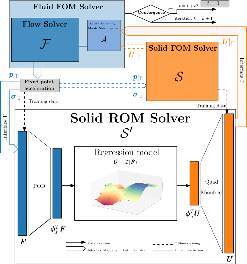
Figure 1: Summarizing illustration of the ROM-FOM approach

3.2 Expected speedups

In this short section, we give an idea of the overall speedup (denoted by $s$) of the partitioned FSI coupling if the solid ROM solver returns a speedup $\sigma$ compared to the solid FOM solver. As mentioned above we will assume that the number of fixed-point subiterations does not vary between FOM-FOM and ROM-FOM strategies. Let us denote by $T_{f}$ (resp. $T_{s}$) the mean computational time taken by the FOM fluid (resp. solid) solver during one time iteration of the FSI coupling. The total FOM-FOM time over a time step is $T_{f}+T_{s}$ while the ROM-FOM time is $T_{f}+T_{s}/\sigma$. The ROM-FOM speedup is then

$$s=\frac{T_{f}+T_{s}}{T_{f}+\dfrac{T_{s}}{\sigma}}=\frac{1+T_{s}/T_{f}}{1+\dfrac{1}{\sigma}T_{s}/T_{f}}.$$

Assume that $T_{s}/T_{f}\gg 1$. Then we get the speedup estimation

$$s\approx\frac{T_{s}/T_{f}}{1+\dfrac{1}{\sigma}T_{s}/T_{f}}=\frac{\sigma}{1+\sigma\dfrac{T_{f}}{T_{s}}}.$$ (22)

Equation (22) shows that a ’good’ solid ROM speedup should be of the order $T_{s}/T_{f}$. Assume for example that $\sigma=T_{s}/T_{f}$, then one finds $s=\sigma/2$ and the efficiency of the ROM-FOM FSI strategy is 1/2. More generally, if the solid ROM achieves a solid speedup $\sigma=\alpha\dfrac{T_{s}}{T_{f}}$ with $\alpha>0$, then

$$s\approx\left(1-\frac{1}{1+\alpha}\right)\,\frac{T_{s}}{T_{f}}.$$

In particular, the ratio $\dfrac{T_{s}}{T_{f}}$ is an upper bound of ROM-FOM FSI speedup.

4 ROM-FOM coupling assessment for low cost FSI simulations

4.1 Model evaluation strategy

In order to evaluate the proposed ROM approach, for multiple parameter values in a training set $\mathcal{P}$, the results of the ROM-FOM simulation will be tested in a future time prediction. In other words, for a given parameter $\boldsymbol{\mu}\in\mathcal{P}\subset\mathcal{D}$, where $\mathcal{D}$ is the convex hull of $\mathcal{P}$, a FOM-FOM simulation will be performed for a specific time period $t\in[0,T]$. After training the ROM on the obtained high fidelity results (including the coupling subiterations), the structural ROM model can be used for $t\in[T,T_{f}]$. In addition, the results associated with all the seen parameters can be used together to train a single ROM, and predict solutions for parameters not seen in training $\hat{\boldsymbol{\mu}}\not\in\mathcal{P}$, and for future time regions $t\in[0,T_{f}]$. In that case, we will also assess the methodology for testing parameters outside the parameter space $\hat{\boldsymbol{\mu}}\not\in\mathcal{D}$. In this work, only parameters associated with the fluid problem are considered. We should note that in the case of time-parameter prediction cases, and in order to avoid ROM-FOM instabilities further down the simulation, the solid FOM needs to be used at some of the first time increments, e.g until a time instant that we will call $T_{i}$, the purpose of this is that on transient cases, the results in the first timesteps are very different than the rest of the simulation, meaning that the training data is much poorer around these values, this results in lower accuracy of the solid ROM, hence it is best to avoid using the ROM in the first transient timesteps. An illustration of this model evaluation strategy applied on the second example can be seen in Figure 10. Simulation data, used for training and testing are available at the Github repositories (ArterialWallROM) and (DoubleFlap) corresponding to the first and second examples respectively.

4.2 Example 1: 1D toy problem of an elastic arterial vessel model

The model of flexible tube and related HF partitioned solvers proposed by Degroote et al. [16] are used here. The flow is assumed to be incompressible with constant density $\rho$. Both fluid mass and momentum conservation equations (neglecting viscosity) read

$$\begin{cases}\partial_{t}a+\partial_{x}(av)=0,\\ \partial_{t}(av)+\partial_{x}(av^{2})+\dfrac{a}{\rho}\,\partial_{x}p=0,\quad t>0,\ x\in[0,L]\end{cases}$$ (23)

where $v$ is the bulk velocity, $a$ is the tube cross section and $p$ is the pressure. From the fluid side, the unknowns are both velocity and pressure. For the solid flexible tube, a quasi-static model

$$a=a(p)$$

is used (retaining only the vessel stress in the circumferential direction). The following nonlinear elastic stress-strain law is used:

$$\begin{cases}\sigma_{\varphi\varphi}=12500\,\epsilon_{\varphi\varphi}\quad\text{if}\ |\epsilon_{\varphi\varphi}|<\epsilon_{0}\\ \sigma_{\varphi\varphi}=2500\,\epsilon_{\varphi\varphi}+20\quad\text{if}\ \epsilon_{\varphi\varphi}\geq\epsilon_{0}\\ \sigma_{\varphi\varphi}=2500\,\epsilon_{\varphi\varphi}-20\quad\text{if}\ \epsilon_{\varphi\varphi}\leq-\epsilon_{0}\\ \end{cases}$$ (24)

with $\epsilon_{0}=2\,\,10^{-3}$. Figure 2 shows a schematic explanation of this problem. For further simplification, a zero pressure condition is applied on the right boundary (note that a non-reflective boundary condition was used in [16]). The prescribed inlet (left face) velocity is computed using the solution of a nonlinear Duffing equation in order to produce a signal with rather complex dynamics.

$$\begin{cases}\ddot{u}(t)=a\,u(t)+b\,u(t)^{2}+c\,u(t)^{3}+d+p\,cos(ft)+e\,\dot{u}(t)\,\,\,\,\forall t\in[0,120]\\ u(0)=10\,\,\,;\,\,\,\dot{u}(0)=0.\\ v_{inlet}(t)=gu(t)+h\\ \end{cases}$$ (25)

We fix $(a,\ b\ ,c\ ,d\ ,e\ ,g\ ,p)=(-1\,\,\,,0\,\,\,,-0.002\,\,\,,-1\,\,\,,-0.02\,\,\,,1/60\,\,\,,360)$ and we parameterize this signal with the parameter vector $\boldsymbol{\mu}=(f\,\,\,,h)^{T}$ allowing the generation of different frequencies and amplitudes.

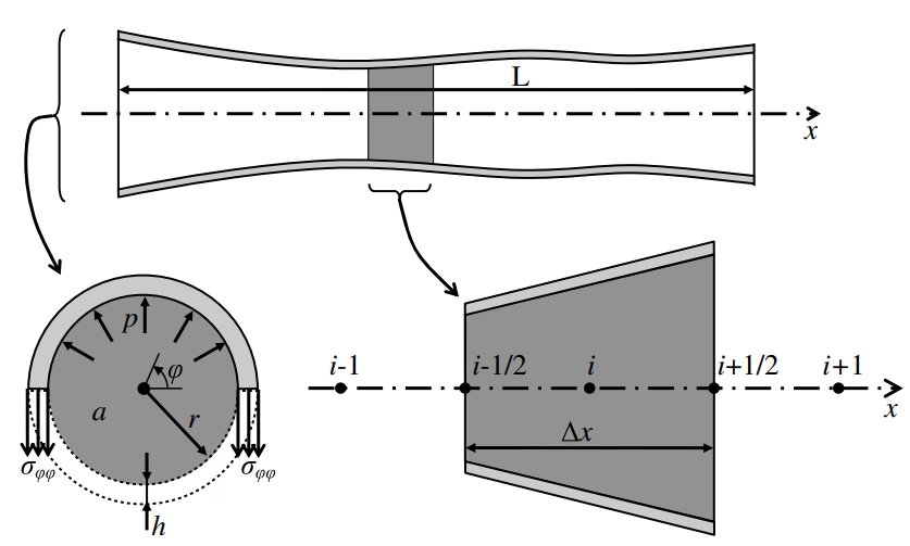
Figure 2: Arterial vessel test case schematic explanation (from [16]). $\sigma_{\varphi\varphi}$ is the vessel hoop stress, $h$ is the thickness and $\Delta x$ is the length of the finite volume cell.

In order to train the ROM model, a FOM-FOM computation is done on a single inlet velocity case corresponding to $\boldsymbol{\mu}_{1}=(2\,\,\,,6)^{T}$ (see Figure 5), for a simulation time period ending in $T=18$ s. The fluid flow equations (23) are solved using a second order finite volume scheme with $100$ cells and the solid section $a(p)$ is computed at each iteration as the solution of a scalar minimization problem. We use the software library preCICE [36] as a coupling interface for the simulations.

For the considered training time region and including all the coupling subiterations, the data is assembled as 737 snapshots ($m=737$ and $N=N_{u}=101$), and $\{\boldsymbol{U},\boldsymbol{F}\}\subset\mathbb{R}^{101\times 737}$.

For this problem, the pressure and section fields are very smooth and only very few modes can model the problem solution. In fact, a $99.99\%$ energy criteria like in (18) implies that only one pressure mode and 5 section modes are needed. Nonetheless, we will use cross-validation to determine an optimal number of modes. A random portion making $20\%$ of the training snapshots will be used as testing samples (denoted as $\boldsymbol{F}_{test}$ and $\boldsymbol{U}_{test}$) and while varying the number of modes of the pressure and section fields, the mean of the $L_{2}$ error on the final output (i.e the section field) will be evaluated upon these samples. In Figure 3, we show a map of the error $\epsilon$ depending on the number of modes, where

$$\epsilon=\frac{1}{m_{test}}\sum_{i}^{m_{test}}||\boldsymbol{U}_{test,i}-ROM(\boldsymbol{F}_{test,i})||_{2}$$ (26)

$m_{test}$ is the number of testing samples and $ROM(\cdot)$ denotes the final output of the trained ROM. Using theses results, we can see that the test error levels off when we reach 9 modes for the section field and 3 modes for the pressure. More precisely, for 9 section modes, we show the evolution of the error $\epsilon$ for different numbers of pressure modes in Figure 4. This also reinforces the idea that this type of cross-validation should be used whenever possible to determine these hyperparameters, since the use of the energy-based criterion only would result in larger error (as seen in Figure 3, the accuracy when using 1 pressure mode and 5 section modes is suboptimal). We note that the displacement reconstruction used here only considers the linear POD terms. In fact, this example being a toy example with the goal of predicting solutions with minimal training data, the training snapshots are not rich enough to accurately learn the quadratic operator $\accentset{\rule{2.79996pt}{0.8pt}}{\boldsymbol{\Phi}}$.

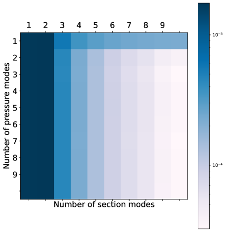
Figure 3: Validation error $\epsilon$ depending on the number of modes choices for both the pressure and the section fields.

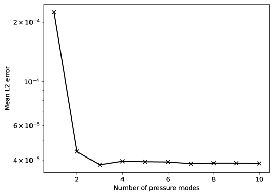
Figure 4: Validation error $\epsilon$ when using 9 section modes depending on the number of pressure modes.

Regarding the regression method, a thin plate spline kernel RBF interpolator is used [37] with

$$\mathcal{I}(\tilde{\boldsymbol{f}})=\sum_{i}^{m}w_{i}\,\phi(||\tilde{\boldsymbol{f}}-\tilde{\boldsymbol{f}}_{i}||)$$ (27)

where

$$\phi(\boldsymbol{x})=\boldsymbol{x}^{2}\log(\boldsymbol{x})$$ (28)

and $\tilde{\boldsymbol{f}}_{i}$ are the RBF centers, chosen as the training points of the reduced forces, resulting eventually in a linear system to be solved for the RBF weights $w_{i}$.

After the ROM has been trained, we test the ROM-FOM coupling on the future prediction with $T_{f}=120$ s at the same inlet velocity. We then choose another parameter vector $\hat{\boldsymbol{\mu}}=(0.9\,\,\,,4)^{T}$ without retraining the ROM, with $T_{i}=0.1$ s We can see the difference between the two signals in Figure 5. The results for theses two cases are shown in Figures 6 and 7 respectively, compared to the HF FOM-FOM solution. We can see a significant accuracy achieved by the suggested ROM-FOM coupling. Moreover, the stress-strain law reconstructed using the ROM-FOM simulation is plotted in Figure 8, showing that the proposed ROM approach can capture the solid problem nonlinearities. Remarkably, we can also see that the ROM-FOM successfully predicted the vessel response in an extrapolated region in the strain response (strain region $\epsilon<-0.0055$) even for this nonlinear constitutive law, although it should be noted that it only involves a linear extrapolation from the phase space seen in the training.

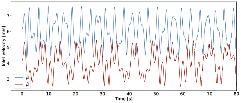
Figure 5: Inlet velocity signals corresponding to $\boldsymbol{\mu}$ and $\hat{\boldsymbol{\mu}}$ parameters values.

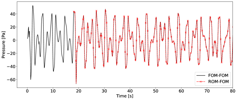
Figure 6: The inlet pressure solution using the FOM-FOM (green dashed line with cross marks) and the ROM-FOM (blue solid line). Prescribed inlet velocity corresponding to $\mu_{1}$. Both training and prediction regimes are depicted. The vertical black line indicates the end of the training time period.

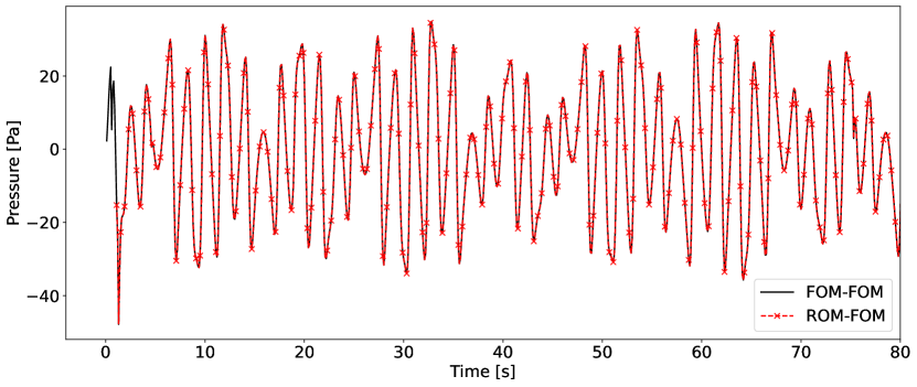
Figure 7: The inlet pressure solution using the FOM-FOM and the ROM-FOM. Prescribed inlet velocity corresponds to $\mu_{2}$. Prediction regime.

In addition, another important property of ROM-FOM coupling schemes is maintaining stability. This directly affects the final ROM speedup, since more instabilities result in an increased number of fixed-point iterations (or even a complete divergence), increasing therefore the overall computational cost. We show in Figure 9 a comparison between the number of iterations until convergence at each time step for both the FOM-FOM and the ROM-FOM models. We observe -as expected- a slight increase in the number of iterations, due to the inaccuracy intrinsic to the reduced model. However, the ROM is accurate enough so that this increase remained limited (approximately $12$ % more iterations at the end) and would not affect the overall speedup in more realistic cases.

The speedup achieved on the structural part for this test case is $\sigma\approx 96$. Nonetheless, there is no expected overall speedup since the fluid model is much more computationally costly than the solid FOM model ($\frac{T_{f}}{T_{s}})\gg 1$. This is however merely a toy problem to evaluate the ROM accuracy and more realistic speedups will be shown in the following example.

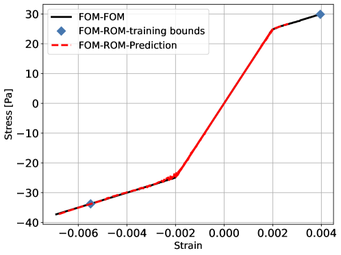
Figure 8: Nonlinear elastic Stress-Strain law used for the vessel tube. The reconstructed curve from the ROM-FOM prediction is plotted along with the FOM-FOM model. We can also see the data points from the FOM-FOM simulation used for the ROM training.

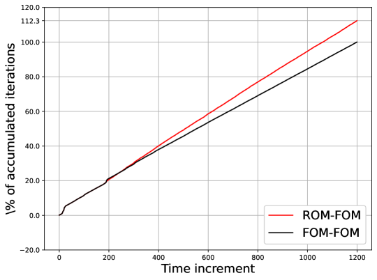
Figure 9: Percentage of the accumulated number of iterations comparing the ROM-FOM to the FOM-FOM.

4.3 Example 2: elastic flaps behind a cylinder wake

In this section, we consider a two-dimensional channel case, where an incompressible flow faces an elastic body with two mounted flap behind a rigid cylinder. We put $\rho=1000\ kg/m^{3}$, $\nu_{f}=0.001\ m^{2}/s$ and a fully developed Poiseuille inlet flow, with a maximum velocity of $v_{max}=2.5\ m/s$ starting from $v=0\ m/s$ at $t=0s$ and increasing linearly until reaching $v_{max}$ at $t=1s$. This corresponds to a Reynolds number of $Re=250$. The boundary condition at the top and bottom walls is a no slip condition, and a homogeneous Neumann boundary condition on the right boundary. A sketch of the test case is given in Figure 2. The solid is governed by a hyperelastic constitutive law, using the Neo-Hookean model, where the stored elastic energy is

$$W(\boldsymbol{F}_{s})=\frac{\mu_{s}}{2}\,(|\boldsymbol{F}_{s}|^{2}-3-2\,\log(J))$$ (29)

where we define $\mu_{s}=\dfrac{E}{2(1+\nu_{s})}$ and we choose $E=10\times 10^{6}$ Pa and $\nu_{s}=0.3$.

The fluid problem is discretised using triangular stabilized finite elements [38] and quadrilateral finite elements are used for the structural problem, with 4 ($X$ and $Y$) displacement degrees of freedom at element nodes. KratosMutiphysics [39] was used as the finite elements software for both problems, using the Kratos modules named FluidDynamicsApplication and StructuralMechanicsApplication in a partitioned coupling. The fluid time step is $dt=0.008$ s. The solid mesh consists of $1805$ nodes with $265$ nodes at the interface, giving $N=530$ and $N_{u}=3610$.

As explained in section 4.1, the Reynolds number $Re$ will be considered as a parameter $\mu$ in this test case. The training set will include 3 points $\mathcal{P}=\{178.6,208.3,250\}$, i.e $\mathcal{D}=[178.6,250]$, and a time domain until $T=3$ s. In addition to time-predictions up to $T_{f}=6$ s, two unseen parameters will be considered, $\hat{\mu}_{1}=192$ $\in\mathcal{D}$ and $\hat{\mu}_{2}=300$ $\not\in\mathcal{D}$, with $T_{i}=0.8$ s. Accordingly, 4 different reduced order models will be assessed: 3 models in a time-prediction setting for each $\mu\in\mathcal{P}$ (hereinafter called ROM 1, ROM 2 and ROM 3 respectively), and the remaining ROM for time-parameter prediction for $\hat{\mu}_{1}$ and $\hat{\mu}_{2}$ (hereinafter called ROM 4). A summary of the ROM evaluation strategy is presented in Figure 10.

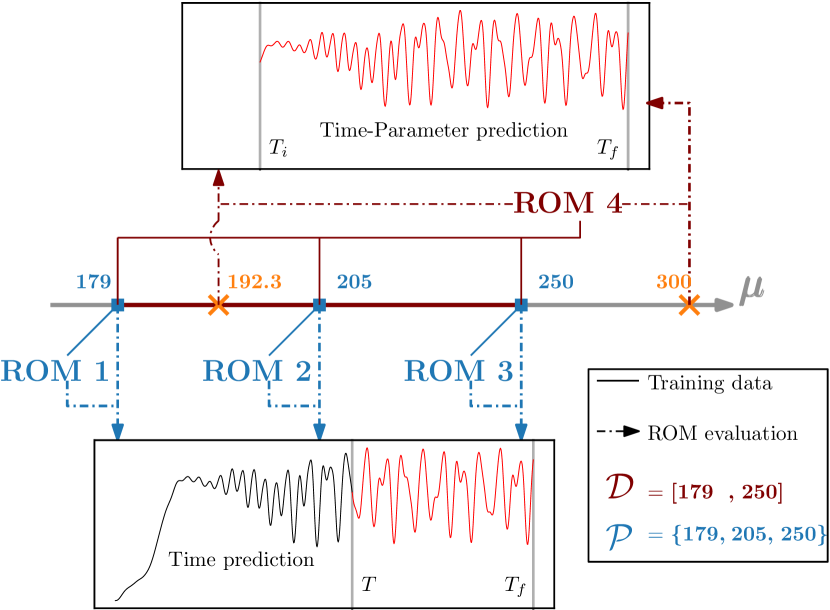
Figure 10: Illustration of trained models and their evaluation strategy.

A total of $6890$ snapshots are used for training corresponding to $2222$, $2311$ and $2357$ snapshots for simulations at $Re$ $\in$ $\{178.6,208.3,250\}$ respectively. In Figure 12, an example of the problem solution at $Re=300$ and $t=3.62$ s is reported for illustration.

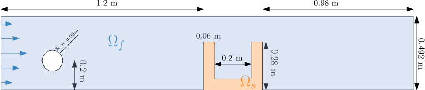
Figure 11: Test case schematic explanation and dimensions.

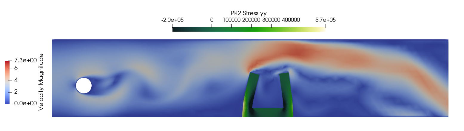
Figure 12: Problem solution at $Re=300$ and $t=3.62$ s. The velocity magnitude is plotted in the fluid domain, while the $yy$ component of the second Piola Kirchoff stress (PK2) is showed in the solid domain.

4.3.1 Dimensionality Reduction

In this case, the forces field on the structural interface has many irregularities that make the linear compression challenging. In Figure 13, we show the energy quantity in the displacement and force fields modes through the singular values of the snapshots matrices. The decay for the forces field is much slower than the one of the displacement field. In order to determine the optimal number of modes used, we use $9$ displacement modes corresponding to $99.99\%$ of the energy, due to the observed fast decay of the singular values. For the forces field, we suggest a cross-validation strategy similar to the one used in the previous test case: $5\%$ of the training data are sampled for testing, and while varying the number of forces modes, the final error of the structural ROM $\varepsilon$ is evaluated as

$$\varepsilon=\left\|\boldsymbol{U}_{test}-ROM(\boldsymbol{F}_{test})\right\|_{2}$$ (30)

Additionally, in order to evaluate the effect of the number of modes on the regression method accuracy, the error of the regression result on the training data $\varepsilon_{regression}$ is also evaluated as

$$\varepsilon_{regression}=||\tilde{\boldsymbol{u}}-\mathcal{I}(\tilde{\boldsymbol{f}})||_{2}$$ (31)

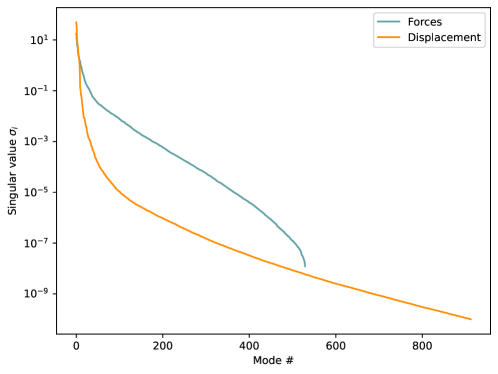
Figure 13: Singular values decay for the displacement and forces snapshots

More details about the regression method used in this test case will be given in the next section. We conservatively choose to pick the maximum of modes between the two criteria. The result of the cross validation is shown in Figure 14 for ROM 4, while the results for the other ROMs are reported in the Appendix. A clear threshold of the accuracy is reached after 45 modes. Indeed, there is a large gap between this choice and the energy-based criteria that results in 36 modes, which shows, again, the importance of this cross-validation step for more optimal choice of hyperparameters.

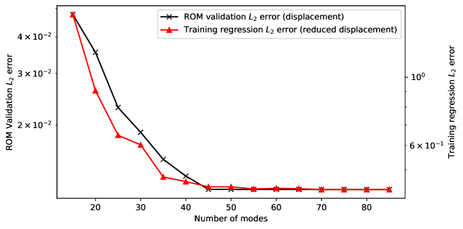
Figure 14: Testing error of the ROM results $\epsilon$ and the regression error on the training data $\epsilon_{regression}$ depending on the number of forces modes. Case of the parametric ROM 4.

4.3.2 Regression method

For this test case, a polynomial regression of degree 2 is used. The Force-Displacement relationship is thus modeled as a second order polynomial:

$$\tilde{\boldsymbol{u}}=\boldsymbol{W}[\tilde{\boldsymbol{f}}\tilde{\otimes}\tilde{\boldsymbol{f}}]$$ (32)

where $\tilde{\otimes}$ is a modified Kronecker product (now different than the product defined in (15) because this product contains the linear terms as well and the intercept term $\boldsymbol{\mathds{1}}$). The polynomial coefficients are arranged in $\boldsymbol{W}\in\mathbb{R}^{r_{u}\times\hat{r}_{f}}$, where $\hat{r}_{f}=(r_{f}+1)(r_{f}+2)/2$ meaning that it scales as $\mathcal{O}(r_{f}^{2})$. We recall that during the cross-validation step $r_{f}$ was chosen as $r_{f}=45$. This means that the number of polynomial coefficients is very large ($\hat{r}_{f}=1081$), and it is highly unlikely that all the polynomial terms are important for modeling $\mathcal{I(\cdot)}$. We thus propose using the Lasso regularization in order to obtain a parsimonious model with as fewest terms as possible, the minimization is written as:

$$\boldsymbol{W}_{i}=arg\min_{\hat{W}_{i}}||\tilde{\boldsymbol{u}}_{i}-\sum_{j=1}^{\hat{r}_{f}}\hat{W}_{ij}[\tilde{\boldsymbol{f}}\otimes\tilde{\boldsymbol{f}}]_{j}||_{2}+\lambda\sum_{j=1}^{\hat{r}_{f}}|\hat{W}_{ij}|\qquad\forall\ i\in\{1\cdots r_{u}\}$$ (33)

where $\boldsymbol{W}_{i}$ and $\boldsymbol{u}_{i}$ are the $i^{th}$ rows and $[\tilde{\boldsymbol{f}}\otimes\tilde{\boldsymbol{f}}]_{j}$ is the $j{th}$ row of the matrices defined in (32). The parameter $\lambda$ promotes the sparsity of the solution $\boldsymbol{W}$ and usually requires fine-tuning. One approach to determine $\lambda$ is to use model selection criteria combined with the LARS algorithm [40] for finding a Lasso solution. This allows the generation of a path of Lasso solutions and the evaluation of criteria, namely the Bayesian information criterion (BIC) along this path. The regularization coefficient $\lambda$ corresponding to the minimum of BIC will be chosen. We use the scikit-learn[41] implementation of this method.

We show in Figure 15 the non-zero terms as a result of the Lasso optimization. We only show the terms associated with the first two outputs (the first two displacement modes) for the model ROM 4. For brevity, the other figures associated with the other ROMs are reported in the Appendix. We can clearly see that only few terms remain after the Lasso optimization. In addition, two important observations are to be made here, the Lasso optimization confirms the necessity of using as much as 45 modes, since many terms associated with these modes are considered. Second, terms associated with interacting modes are also important, showing that modeling the nonlinearity of the force-displacement relationship as a second-degree polynomial function is indeed an adequate choice.

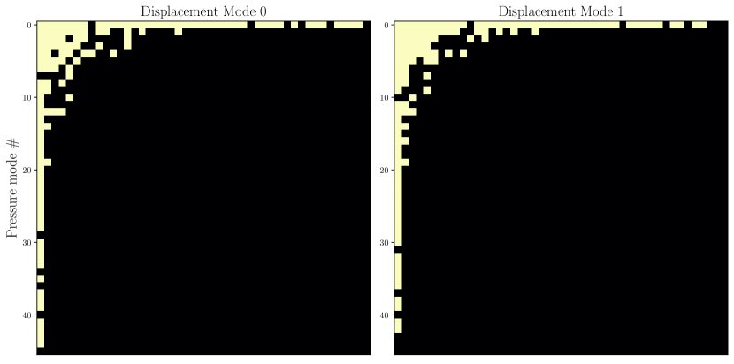
Figure 15: Illustration of the non-zero terms (yellow pixels) among all the $2^{nd}$ degree polynomial terms. Each row/column represents a pressure mode so that the $ij$ pixel represents the term corresponding to the product of $i^{th}$ mode with $j^{th}$ mode, while the mode $0$ represents the term $1$. Case of ROM 4 and the first two displacement modes.

4.3.3 ROM-FOM coupling accuracy and speedup

The ROM 4 evaluation results are shown in Figure 17 where we show the time evolution of the left-most solid tip $x$-displacement, and similarly for the right-most tip in 18. We also show the same results in a time-prediction setting using ROM 1 in Figure 19. The complete deformation with a map of the PK2 stress field is shown for both the FOM and ROM results in Figure 16. The relative $L_{2}$ error on the complete displacement field defined as

$$e(t)=\frac{||\boldsymbol{U}(t)-\hat{\boldsymbol{U}}(t)||_{2}}{<{||\boldsymbol{U}(t)||_{2}}>}$$ (34)

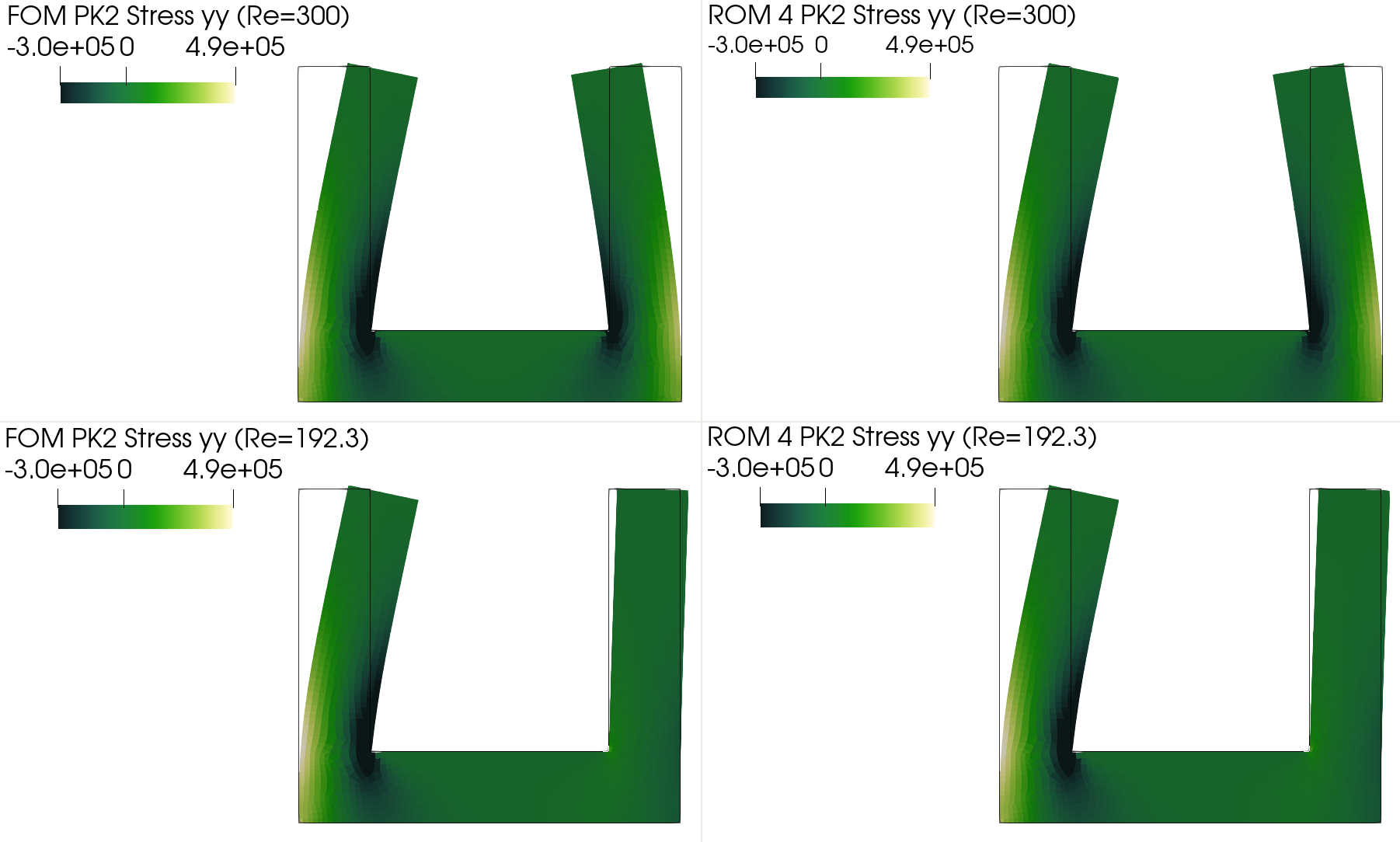
Figure 16: The ROM-FOM (using ROM 4) results compared to the FOM-FOM results. This is taken at $t=5.84$ s. The $yy$ component of the PK2 stress field is showed while also showing the complete solid deformation.

is also shown in Figure 21. A highly accurate prediction of the ROM-FOM model is obtained for each case. For the unseen parameter outside the training space $\mathcal{D}$ ($Re=300)$, the error is larger, but remains under 10$\%$ for the considered time region. Remarkably, in the case of ROM 1, ROM 2 and ROM 3, where the training was done on a single parameter and where the evaluation was done on an unseen time range, only $4\%$ of error is observed, despite the complex dynamics. To further highlight this, we show the displacement phase-space ($u_{L}(t)$, $u_{R}(t)$) in Figure 20, where $u_{L}(t)$ is the left-most node displacement and $u_{R}(t)$ is the right-most node displacement. More precisely, we show the space seen in training (Top) and the one seen in the testing phase (Bottom) in the case of ROM 3. This figure demonstrates a good agreement between the FOM-FOM and ROM-FOM results. Again, the complexity of the dynamics is well handled since a high-fidelity FOM is kept on the fluid part. We argue that as long as the amplitudes of the fluid forces are close to those seen in training, the proposed ROM strategy will enable a good prediction accuracy, even when extrapolating in time and parametric space, at least when the flow regime remains the same.

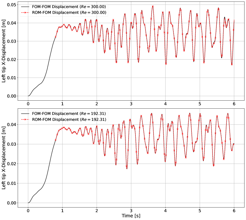
Figure 17: The ROM-FOM left tip x-displacement of the solid body using ROM 4 (evaluated at $Re=192$ and $Re=300$), compared to the FOM-FOM solution.

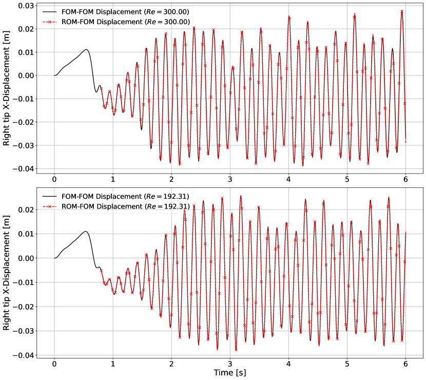
Figure 18: The ROM-FOM right tip x-displacement of the solid body using ROM 4 (evaluated at $Re=192$ and $Re=300$), compared to the FOM-FOM solution.

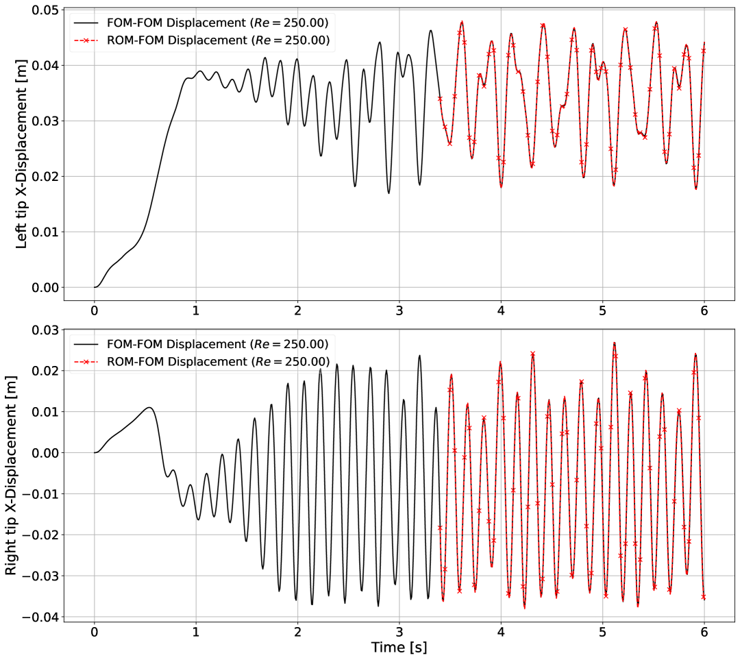
Figure 19: The ROM-FOM left tip x-displacement of the solid body using ROM 3 compared to the FOM-FOM solution.

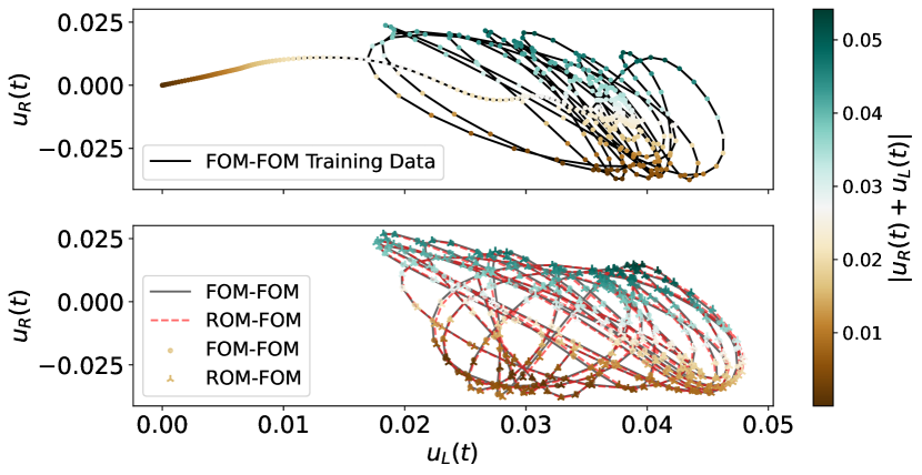
Figure 20: The X-displacement phase space ($u_{L}(t)$, $u_{R}(t)$) where $u_{L}(t)$ is the left-most node displacement and $u_{L}(t)$ is the right-most node displacement. Top: Trajectory seen in training ($Re=250$). Bottom: A comparison between the FOM-FOM (black line) and ROM-FOM (red dashed line) results. Case of ROM 3

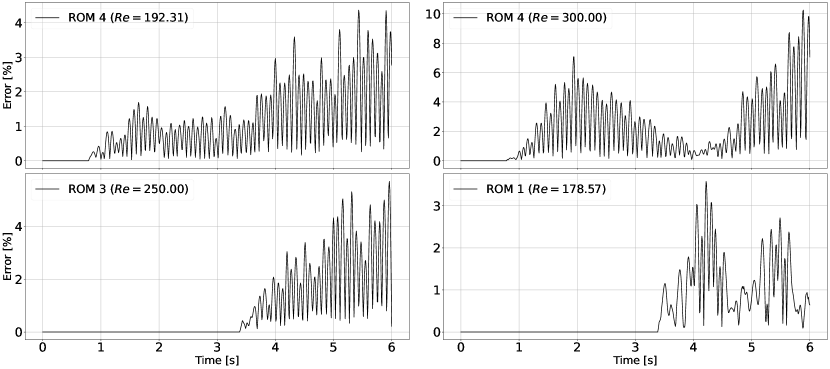
Figure 21: The ROM-FOM $L_{2}$ error $e(t)$ as defined in (34) for the previous cases.

As an indicator of the ROM-FOM stability, in Figure 22, we show the number of coupling iterations needed to convergence, compared to the FOM-FOM results. We see only $7\%$ additional iterations in the case of ROM 4 evaluation at $Re=300$. The other cases are reported in the Appendix. Such a slight increase in the overall coupling iterations show the good stability of the ROM-FOM scheme, due to the high accuracy of the solid ROM.

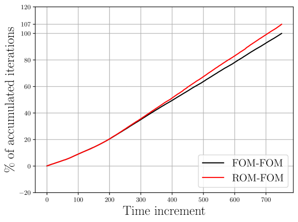
Figure 22: Accumulated number of iterations in a comparison between the ROM-FOM and FOM-FOM results. Case of ROM 4 evaluated at $Re=300$

On an 8-Cores Mac M1 laptop, the CPU time of the ROM solid solver is on average (case of ROM 4 at $Re=300$) $0.0028\;s$ as opposed to $T_{s}=0.724\;s$ for the solid FOM solver, making the speedup obtained for the solid problem $\sigma\approx 260$. The total CPU time for the complete FOM-FOM simulation is $5763\;s$ and $3181\;s$ for the ROM-FOM simulation, making the overall speedup for the FSI simulation around $s\approx 1.81$. We should note that the ratio $\frac{T_{f}}{T_{s}}$ varies during the simulation, since the internal solvers’ convergence takes different number of nonlinear iterations depending on the simulation time steps. For a more detailed analysis, we show in Figure 23 the ratio $\frac{T_{f}}{T_{s}}$ for every subiterations and its distribution, while comparing both models, we can see the large difference when modifying the solid solver to make it much faster than the fluid solver. Average speedups and CPU time of training the ROMs are reported in the Appendix.

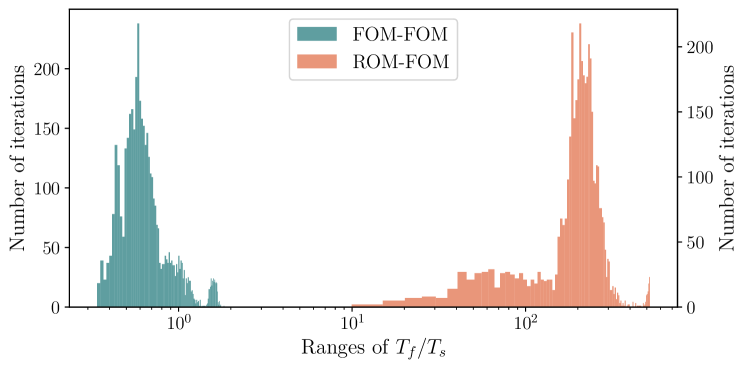
Figure 23: Distribution of the ratios of CPU time $\frac{T_{f}}{T_{s}}$ for all subiterations for both the ROM-FOM to the FOM-FOM strategies.

5 Conclusions

We have presented a ROM-FOM coupling strategy designed to reduce the computational cost of partitioned FSI simulations, through the reduction of the solid sub-problem. The proposed approach is data-driven, can be implemented in a completely non-intrusive framework, and is well-suited for nonlinear elastic solid problems under quasi-static load. Using a dimensionality reduction of the fluid forces as well as the displacement field on linear subspaces, a regression model between the two fields is constructed in the latent space, followed by a reconstruction towards the high-dimensional space of the displacement field using a quadratic manifold approximation, for a reconstruction as much accurate as possible. The obtained ROM can accurately predict the full displacement field online with a significant speedup compared to the reference FOM-FOM solution. The performance of the proposed ROM strategy has been demonstrated on two different test cases where we have shown a significant accuracy of the ROM-FOM coupling even for complex dynamics tracking. Finally, the proposed methodology was shown to perform very well in both time and parametric extrapolated region space. Despite the novelty of this type of ROM-FOM coupling scheme, and its significant potential for application on many common FSI problems, improvements can still be made to enhance the robustness of this method. For example, further understanding of the instability of the FSI simulations - a property intrinsic to the partitioned coupling schemes - will allow a better design of the structural ROMs, avoiding additional coupling iterations, and achieving better speedups. Nonlinear dimensionality reduction methods, especially for the fluid forces field, could also make the ROM less complex while maintaining good generalization properties. Additionally, multidimensional parametric spaces, including parameters of the solid problem itself (e.g material constitutive law parameters) will also be investigated in the future.

6 Acknowledgements

This work has been funded by the ANR (Agence Nationale de la Recherche), Altair Engineering and Michelin.

Appendix A Appendix: Figures for detailed results of the constructed ROMs

A.1 Choices of number of forces modes:

As explained in section 4.3.1, a cross-validation is done for every ROM training, in order to find the optimal latent dimension of the fluid forces subspace, the results for ROM 4 having been showed in Figure 14, the results for the other ROMs will be shown in the following Figure 24. These results and the energy-criterion for the displacement modes give the optimal choices that are summarized in Table 1

Table 1: Cross validation results.

	ROM 1	ROM 2	ROM 3	ROM 4
# of modes of F	45	40	50	45
# of modes of U	9

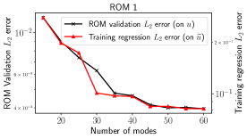
(a) ROM 1 case

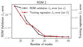
(b) ROM 2 case

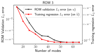
(c) ROM 3 case

Figure 24: Testing error of the ROM results $\epsilon$ and $\epsilon_{regression}$ for cross-validation.

A.2 Polynomial terms after the Lasso optimization:

Similarly to Figure 15, we show the equivalent results for the other trained ROMs.

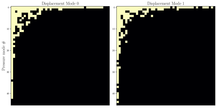
Figure 25: Non-zero polynomial terms. ROM 1

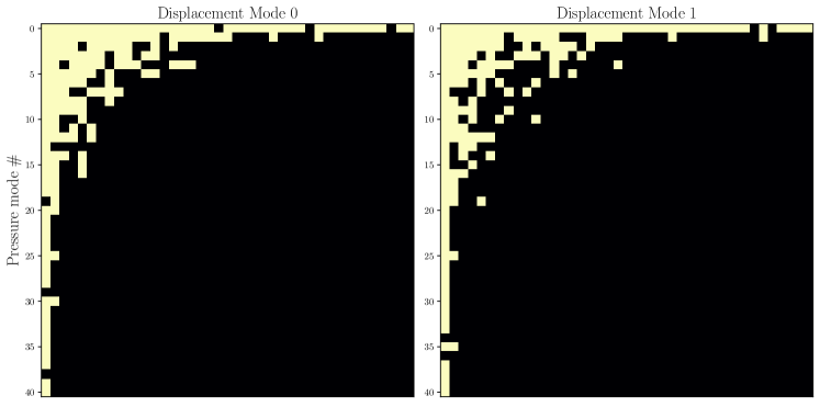
Figure 26: Non-zero polynomial terms. ROM 2

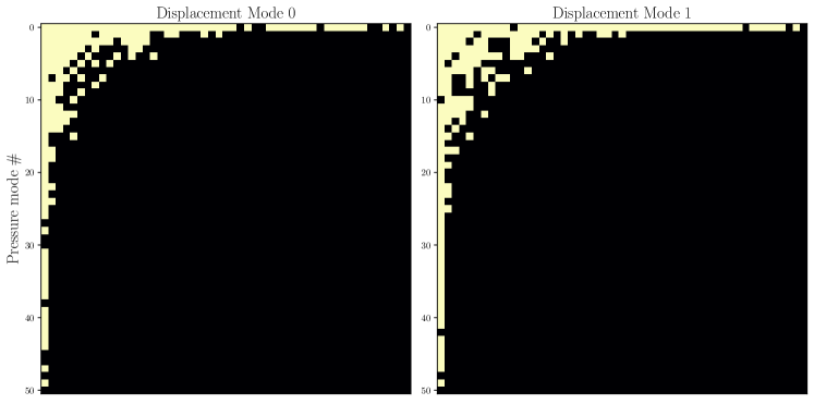
Figure 27: Non-zero polynomial terms. ROM 3

A.3 ROM evaluation: Displacement results:

We show in the following Figure 28 the results of the ROM-FOM and FOM-FOM comparisons in terms of displacement values at the tips of the structure.

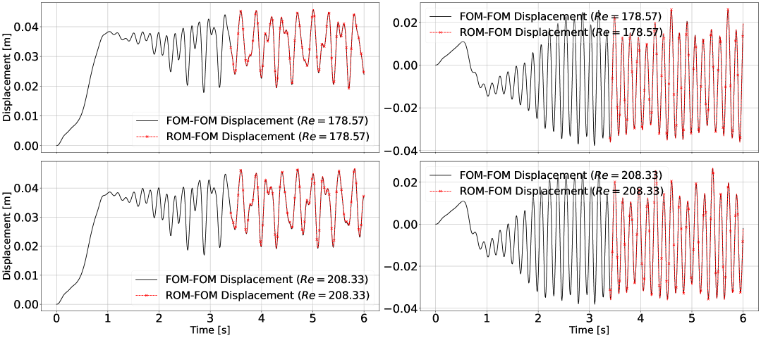
Figure 28: The ROM-FOM tips x-displacement of the solid body compared to the FOM-FOM solution. Top: case of ROM 1 - Bottom: case of ROM 2. Left: Left-most tip - Right: Right-most tip

A.4 ROM evaluation: Coupling iterations:

Similarly to Figure 22, we show the coupling iterations comparison for the other ROMs in Figure 29.

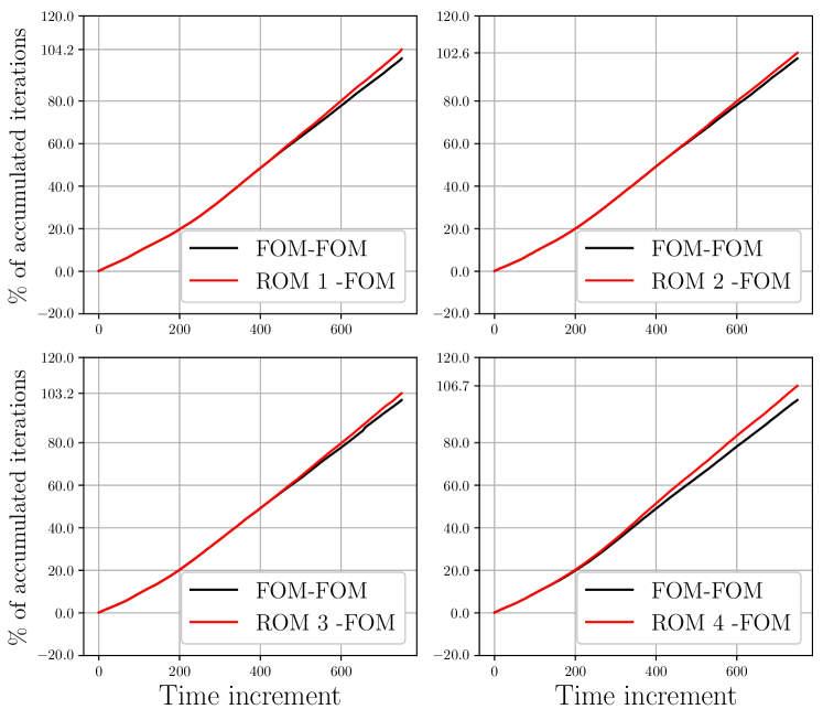
Figure 29: Comparison of total fixed-point iterations between the FOM-FOM and ROM-FOM for ROM 1, ROM 2, ROM 3 and ROM 4 (at $Re=192.3$)

A.5 ROM evaluation: Speedups:

In this section, we show the average speedup - On an 8-Cores Mac M1 laptop with a $16$ GB RAM - achieved by the ROM, on the structural solver itself and on the total simulation. We note that the displacement field reconstruction (15) is taken into account in the ROM computation time.

Table 2: Speedup results.

	ROM 1	ROM 2	ROM 3	ROM 4 ($Re=192.3$)	ROM 4 ($Re=300$)
Training time [s]	20.98	22.08	33.55	52.77
(Training+Cross validation) time [s]	181.9	188.12	242.12	1348.58
Average solid speedup	236.35	183.64	250.75	239.51	259.78
Total speedup	1.814	1.88	1.795	1.656	1.81

References

- Donea et al. [1982] J. Donea, S. Giuliani, J. P. Halleux, An arbitrary lagrangian-eulerian finite element method for transient dynamic fluid-structure interactions, Computer Methods in Applied Mechanics and Engineering 33 (1982) 689–723. doi:10.1016/0045-7825(82)90128-1.
- Morton et al. [1998] S. A. Morton, R. B. Melville, M. R. Visbal, Accuracy and Coupling Issues of Aeroelastic Navier-Stokes Solutions on Deforming Meshes, Journal of Aircraft 35 (1998) 798–805. doi:10.2514/2.2372, publisher: American Institute of Aeronautics and Astronautics.
- Bathe and Zhang [2004] K.-J. Bathe, H. Zhang, Finite element developments for general fluid flows with structural interactions: GENERAL FLUID FLOWS WITH STRUCTURAL INTERACTIONS, International Journal for Numerical Methods in Engineering 60 (2004) 213–232. doi:10.1002/nme.959.
- Heil [2004] M. Heil, An efficient solver for the fully coupled solution of large-displacement fluid–structure interaction problems, Computer Methods in Applied Mechanics and Engineering 193 (2004) 1–23. doi:10.1016/j.cma.2003.09.006.
- Fernández and Gerbeau [2009] M. A. Fernández, J.-F. Gerbeau, Algorithms for fluid-structure interaction problems, in: L. Formaggia, A. Quarteroni, A. Veneziani (Eds.), Cardiovascular Mathematics: Modeling and simulation of the circulatory system, Springer Milan, Milano, 2009, pp. 307–346.
- Uekermann [2016] B. Uekermann, Partitioned Fluid-Structure Interaction on Massively Parallel Systems, Ph.D. thesis, TUM, 2016.
- Bogaers et al. [2014] A. E. J. Bogaers, S. Kok, B. D. Reddy, T. Franz, Quasi-Newton methods for implicit black-box FSI coupling, Computer Methods in Applied Mechanics and Engineering 279 (2014) 113–132. doi:10.1016/j.cma.2014.06.033.
- Guruswamy [1990] G. P. Guruswamy, Unsteady aerodynamic and aeroelastic calculations for wings using Euler equations, AIAA Journal 28 (1990) 461–469. doi:10.2514/3.10415, publisher: American Institute of Aeronautics and Astronautics.
- Piperno et al. [1995] S. Piperno, C. Farhat, B. Larrouturou, Partitioned procedures for the transient solution of coupled aroelastic problems Part I: Model problem, theory and two-dimensional application, Computer Methods in Applied Mechanics and Engineering 124 (1995) 79–112. doi:10.1016/0045-7825(95)92707-9.
- Farhat and Lesoinne [2000] C. Farhat, M. Lesoinne, Two efficient staggered algorithms for the serial and parallel solution of three-dimensional nonlinear transient aeroelastic problems, Computer Methods in Applied Mechanics and Engineering 182 (2000) 499–515. doi:10.1016/S0045-7825(99)00206-6.
- Lesoinne and Farhat [1996] M. Lesoinne, C. Farhat, Geometric conservation laws for flow problems with moving boundaries and deformable meshes, and their impact on aeroelastic computations, Computer Methods in Applied Mechanics and Engineering 134 (1996) 71–90. doi:10.1016/0045-7825(96)01028-6.
- Nobile [2001] F. Nobile, Numerical approximation of fluid-structure interaction problems with application to haemodynamics, Ph.D. thesis, EPFL, Lausanne, 2001. doi:10.5075/epfl-thesis-2458.
- Causin et al. [2005] P. Causin, J. F. Gerbeau, F. Nobile, Added-mass effect in the design of partitioned algorithms for fluid–structure problems, Computer Methods in Applied Mechanics and Engineering 194 (2005) 4506–4527. doi:10.1016/j.cma.2004.12.005.
- Felippa et al. [2001] C. A. Felippa, K. C. Park, C. Farhat, Partitioned analysis of coupled mechanical systems, Computer Methods in Applied Mechanics and Engineering 190 (2001) 3247–3270. doi:10.1016/S0045-7825(00)00391-1.
- Degroote et al. [2009] J. Degroote, K.-J. Bathe, J. Vierendeels, Performance of a new partitioned procedure versus a monolithic procedure in fluid–structure interaction, Computers & Structures 87 (2009) 793–801. doi:10.1016/j.compstruc.2008.11.013.
- Degroote et al. [2008] J. Degroote, P. Bruggeman, R. Haelterman, J. Vierendeels, Stability of a coupling technique for partitioned solvers in FSI applications, Computers & Structures 86 (2008) 2224–2234. doi:10.1016/j.compstruc.2008.05.005.
- Sirovich [1987] L. Sirovich, Turbulence and the dynamics of coherent structures. II. Symmetries and transformations, Quarterly of Applied Mathematics 45 (1987) 573–582. doi:10.1090/qam/910463.
- Lassila et al. [2014] T. Lassila, A. Manzoni, A. Quarteroni, G. Rozza, Model Order Reduction in Fluid Dynamics: Challenges and Perspectives, in: A. Quarteroni, G. Rozza (Eds.), Reduced Order Methods for Modeling and Computational Reduction, MS&A - Modeling, Simulation and Applications, Springer International Publishing, Cham, 2014, pp. 235–273.
- Bui-Thanh et al. [2008] T. Bui-Thanh, K. Willcox, O. Ghattas, Parametric Reduced-Order Models for Probabilistic Analysis of Unsteady Aerodynamic Applications, AIAA Journal 46 (2008) 2520–2529. doi:10.2514/1.35850, publisher: American Institute of Aeronautics and Astronautics.
- Veroy et al. [2012] K. Veroy, C. Prud’homme, D. Rovas, A. Patera, A Posteriori Error Bounds for Reduced-Basis Approximation of Parametrized Noncoercive and Nonlinear Elliptic Partial Differential Equations, in: 16th AIAA Computational Fluid Dynamics Conference, American Institute of Aeronautics and Astronautics, 2012. doi:10.2514/6.2003-3847.
- Shinde et al. [2019] V. Shinde, E. Longatte, F. Baj, Y. Hoarau, M. Braza, Galerkin-free model reduction for fluid-structure interaction using proper orthogonal decomposition, Journal of Computational Physics 396 (2019) 579–595. doi:10.1016/j.jcp.2019.06.073.
- Xiao et al. [2016] D. Xiao, P. Yang, F. Fang, J. Xiang, C. C. Pain, I. M. Navon, Non-intrusive reduced order modelling of fluid–structure interactions, Computer Methods in Applied Mechanics and Engineering 303 (2016) 35–54. doi:10.1016/j.cma.2015.12.029.
- Fresca and Manzoni [2022] S. Fresca, A. Manzoni, POD-DL-ROM: Enhancing deep learning-based reduced order models for nonlinear parametrized PDEs by proper orthogonal decomposition, Computer Methods in Applied Mechanics and Engineering 388 (2022) 114181. doi:10.1016/j.cma.2021.114181.
- Gupta and Jaiman [2022] R. Gupta, R. Jaiman, A hybrid partitioned deep learning methodology for moving interface and fluid–structure interaction, Computers & Fluids 233 (2022) 105239. doi:10.1016/j.compfluid.2021.105239.
- Miyanawala and Jaiman [2019] T. P. Miyanawala, R. K. Jaiman, A Hybrid Data-Driven Deep Learning Technique for Fluid-Structure Interaction, in: ASME 2019 38th International Conference on Ocean, Offshore and Arctic Engineering, American Society of Mechanical Engineers Digital Collection, 2019. doi:10.1115/OMAE2019-95870.
- Lee et al. [2023] S. Lee, K. Jang, S. Lee, H. Cho, S. Shin, Parametric model order reduction by machine learning for fluid–structure interaction analysis, Engineering with Computers (2023). doi:10.1007/s00366-023-01782-2.
- Zhang et al. [2022] X. Zhang, T. Ji, F. Xie, C. Zheng, Y. Zheng, Data-driven nonlinear reduced-order modeling of unsteady fluid–structure interactions, Physics of Fluids 34 (2022) 053608. doi:10.1063/5.0090394.
- Totounferoush et al. [2021] A. Totounferoush, A. Schumacher, M. Schulte, Partitioned deep learning of fluid-structure interaction, CoRR abs/2105.06785 (2021). arXiv:2105.06785.
- Fries et al. [2022] W. D. Fries, X. He, Y. Choi, LaSDI: Parametric Latent Space Dynamics Identification, Computer Methods in Applied Mechanics and Engineering 399 (2022) 115436. doi:https://doi.org/10.1016/j.cma.2022.115436.
- Guo and Hesthaven [2018] M. Guo, J. S. Hesthaven, Reduced order modeling for nonlinear structural analysis using Gaussian process regression, Computer Methods in Applied Mechanics and Engineering 341 (2018) 807–826. doi:10.1016/j.cma.2018.07.017.
- Brunton et al. [2016] S. L. Brunton, J. L. Proctor, J. N. Kutz, Discovering governing equations from data by sparse identification of nonlinear dynamical systems, Proceedings of the National Academy of Sciences 113 (2016) 3932–3937. doi:10.1073/pnas.1517384113, publisher: Proceedings of the National Academy of Sciences.
- Andrés Arcones et al. [2022] D. Andrés Arcones, R. Ellath Meethal, B. Obst, R. Wüchner, Neural network-based surrogate models applied to fluid-structure interaction problems, 2022. doi:10.23967/wccm-apcom.2022.080.
- Haelterman et al. [2016] R. Haelterman, A. E. J. Bogaers, K. Scheufele, B. Uekermann, M. Mehl, Improving the performance of the partitioned QN-ILS procedure for fluid–structure interaction problems: Filtering, Computers & Structures 171 (2016) 9–17. doi:10.1016/j.compstruc.2016.04.001.
- Geelen et al. [2023] R. Geelen, S. Wright, K. Willcox, Operator inference for non-intrusive model reduction with quadratic manifolds, Computer Methods in Applied Mechanics and Engineering 403 (2023) 115717. doi:10.1016/j.cma.2022.115717.
- Wahba [1990] G. Wahba, Spline Models for Observational Data, CBMS-NSF Regional Conference Series in Applied Mathematics, Society for Industrial and Applied Mathematics, 1990. doi:10.1137/1.9781611970128.
- Chourdakis et al. [2022] G. Chourdakis, K. Davis, B. Rodenberg, et al., precice v2: A sustainable and user-friendly coupling library, Open Research Europe 2 (2022). doi:10.12688/openreseurope.14445.2.
- Wood [2003] S. N. Wood, Thin Plate Regression Splines, Journal of the Royal Statistical Society Series B: Statistical Methodology 65 (2003) 95–114. doi:10.1111/1467-9868.00374.
- Codina [2001] R. Codina, A stabilized finite element method for generalized stationary incompressible flows, Computer Methods in Applied Mechanics and Engineering 190 (2001) 2681–2706. doi:10.1016/S0045-7825(00)00260-7.
- Dadvand et al. [2010] P. Dadvand, R. Rossi, E. Oñate, An Object-oriented Environment for Developing Finite Element Codes for Multi-disciplinary Applications, Arch Computat Methods Eng 17 (2010) 253–297. doi:10.1007/s11831-010-9045-2.
- Efron et al. [2004] B. Efron, T. Hastie, I. Johnstone, R. Tibshirani, Least angle regression, The Annals of Statistics 32 (2004) 407 – 499. doi:10.1214/009053604000000067.
- Pedregosa et al. [2011] F. Pedregosa, G. Varoquaux, A. Gramfort, V. Michel, B. Thirion, O. Grisel, M. Blondel, P. Prettenhofer, R. Weiss, V. Dubourg, J. Vanderplas, A. Passos, D. Cournapeau, M. Brucher, M. Perrot, Édouard Duchesnay, Scikit-learn: Machine learning in python, Journal of Machine Learning Research 12 (2011) 2825–2830. URL: http://jmlr.org/papers/v12/pedregosa11a.html.