Learning under Selective Labels with Data from Heterogeneous Decision-makers: An Instrumental Variable Approach

Abstract

We study the problem of learning with selectively labeled data, which arises when outcomes are only partially labeled due to historical decision-making. The labeled data distribution may substantially differ from the full population, especially when the historical decisions and the target outcome can be simultaneously affected by some unobserved factors. Consequently, learning with only the labeled data may lead to severely biased results when deployed to the full population. Our paper tackles this challenge by exploiting the fact that in many applications the historical decisions were made by a set of heterogeneous decision-makers. In particular, we analyze this setup in a principled instrumental variable (IV) framework. We establish conditions for the full-population risk of any given prediction rule to be point-identified from the observed data and provide sharp risk bounds when the point identification fails. We further propose a weighted learning approach that learns prediction rules robust to the label selection bias in both identification settings. Finally, we apply our proposed approach to a semi-synthetic financial dataset and demonstrate its superior performance in the presence of selection bias.

1 Introduction

The problem of selective labels is common in many decision-making applications involving human subjects. In these applications, each individual receives a certain decision that in turn determines whether the individual’s outcome label is observed. For example, in judicial bail decision-making, the outcome of interest is whether a defendant returns to the court without comitting another crime were the defendant released. But this outcome cannot be observed if the bail is denied. In lending, the default status of a loan applicant cannot be observed if the loan application is not approved. In hiring, a candidate’s job performance cannot be observed if the candidate is not hired.

The selective label problem poses serious challenges to develop effective machine learning algorithms to aid decision-making [Lakkaraju et al., 2017, Kleinberg et al., 2018]. Indeed, the labeled data may not be representative of the full population that will receive the decisions, which is also known as a selection bias problem. As a result, good performance on the labeled subjects may not translate into good performance for the full population, and machine learning models trained on the selectively labeled data may perform poorly when deployed in the wild. This is particularly concerning when historical decisions depended on unobservable variables not recorded in the data, as is often the case when historical decisions were made by humans. Then the labeled data and the full population can differ substantially in terms of factors unknown to the machine learning modelers.

In this paper, we tackle the selective label problem by exploiting the fact that in many applications the historical decisions were made by multiple decision-makers. In particular, the decision-makers are heterogenous in that they have different decision rules and may make different decision to the same unit. Moreover, the decision-makers face similar pools of subjects so that each subject can be virtually considered as randomly assigned to one decision-maker. This structure provides opportunities to overcome the selective label problem, since an unlabelled subject could have otherwise been assigned to a different decision-maker and been labeled. For example, judicial decisions are often made by multiple judges. They may have different degrees of leniency in releasing the same defendant. This heterogeneous decision-maker structure has been also used in the existing literature to handle selection bias [e.g., Lakkaraju et al., 2017, Kleinberg et al., 2018, Rambachan et al., 2021, Arnold et al., 2022].

To harness the decision-maker heterogeneity, we view the decision-maker assignment as an instrumental variable (IV) for the historical decision subject to selection bias. We thoroughly study the evaluation of machine learning prediction algorithms from an identification perspective (see Section 3). We provide a sufficient condition for the prediction risk of an algorithm over the full population to be uniquely identified (i.e., point-identified) from the observed data. We show that the sufficient condition is very strong and the full-population prediction risk may often be unidentifiable. Thus we alternatively provide tight bounds on the full-population prediction risk under a mild condition. This lack of identification highlights intrinsic ambiguity in algorithm evaluation with selective labels, explaining why the heuristic single-valued point evaluation estimators in Lakkaraju et al. [2017], Kleinberg et al. [2018] tend to be biased (see Section 3.3).

We further develop an algorithm to learn a prediction rule from data (see Section 4). This complements the existing selective label literature that mostly focuses on the robust evaluation of machine learning models [e.g., Lakkaraju et al., 2017, Kleinberg et al., 2018, among others reviewd in Section 1.1], but the models are often directly trained on biased labeled data to begin with. In this paper, we seek robustness not only in evaluation but also in the model training. Our proposed learning algorithm builds on our our identification results and apply both when the full-population prediction risk is point-identified and when it is only partially identified. It is based on a unified weighted classification procedure that can be efficiently implemented via standard machine learning packages. We demonstrate the performance of our proposed algorithm in Section 6 and theoretically bound its generalization error in Section 5.

1.1 Related Work

Our work is directly related to the growing literature on the selective label problem. Kleinberg et al. [2018], Lakkaraju et al. [2017] formalize the problem in the machine learning context and leverage the decision-maker heterogeneity via a heuristic “contraction” technique. Rambachan et al. [2022] provide formal identification analysis and derive partial identification bounds on multiple model accuracy measures in a variety of settings, including the setting with decision-maker assignment IV. See Section 3.3 for a more detailed comparison of our work with these papers. Some recent papers also tackle the selective label problem by leveraging alternative information. For example, De-Arteaga et al. [2018, 2021] propose to impute missing labels when human decision-makers reach concensus decisions. Laine et al. [2020] propose a Bayesian approach under simplified parametric models. Bertsimas and Fazel-Zarandi [2022] uses a geographic proximity instrumental variable in a immigration law enforcement application. Notably, all of these papers only focus on model evaluation, while our paper also studies model learning. Finally, we note that a few recent papers study the selective label problem in an online learning setting [Kilbertus et al., 2020, Wei, 2021, Ben-Michael et al., 2021, Yang et al., 2022], while we focus on an offline setting.

Our work builds on the IV literature in statistics and econometrics. IV is a common and powerful tool to handle unmeasured confounding in causal inference [e.g., Angrist and Pischke, 2009, Angrist and Imbens, 1995, Angrist et al., 1996]. Actually, some empirical studies have already considered heterogenous decision-makers as an IV, such as the judge IV in Kling [2006], Mueller-Smith [2015]. However, these analyses are based on linear parametric models, while our identification analysis is free of any parametric restrictions.

Our point identification analysis builds on Wang and Tchetgen [2018], Cui and Tchetgen Tchetgen [2021] and our partial identification analysis builds on Manski and Pepper [1998], Swanson et al. [2018], Balke and Pearl [1994]. Our paper directly extends these results to the evaluation of prediction risks under selective labels, and develop novel reformulations that enable efficient learning of prediction rules via a unified procedure.

Our work is also tied to the literature of learning individualized treatment rules (ITR) [e.g., Zhao et al., 2012, Kosorok and Laber, 2019, Qian and Murphy, 2011]. Particularly relevant to our work are Cui and Tchetgen Tchetgen [2021], Pu and Zhang [2021], who study ITR learning with instrumental variables in the point identification setting and partial identification setting respectively. They consider a causal problem with a binary treatment variable and a binary IV, while we consider a selective label problem with a multi-valued IV. Moreover, our paper features a unified solution to learning in both identification settings.

2 Problem Formulation

We now formalize the problem of selective labels. Consider a sample of $i=1,\dots,n$ units. For each unit $i$, we let $Y_{i}^{*}\in\{0,1\}$ denote the true outcome of interest, and $X_{i}\in\mathcal{X}$ and $U_{i}\in\mathcal{U}$ denote certain observable and unobservable features that may be strongly dependent with $Y_{i}^{*}$. However, the true outcome $Y_{i}^{*}$ is not fully observed. Instead, the observability of $Y_{i}^{*}$ depends on a binary decision $D_{i}\in\{0,1\}$ made by a human decision-maker $Z_{i}\in[m]\coloneqq\{1,\dots,m\}$ according to the features $(X_{i},U_{i})$. Specifically, the observed outcome $Y_{i}\in\{1,0,\text{NA}\}$ (where NA stands for a missing value) is given as follows:

$$Y_{i}=\left\{\begin{aligned} &Y_{i}^{*}\quad&&D_{i}=1,\\ &\text{NA}\quad&&D_{i}=0.\\ \end{aligned}\right.$$

In other words, each unit’s outcome is selectively labeled according to the binary decision. We assume that $(Y_{i},Y^{*}_{i},D_{i},Z_{i},X_{i},U_{i})$ for $i=1,\dots,n$ are independent and identically distributed draws from a common population $(Y,Y^{*},D,Z,X,U)$. The observed sample is given by $S_{n}=\{(Y_{i},D_{i},X_{i},Z_{i}),i=1,\dots,n\}$. Figure 1 shows an example causal graph for the variables.

Figure 1: Causal graph of selective labels problem

The selective label problem is prevalent in various scenarios, including the judicial bail problem where judges must determine defendant release. For each defendant $i$, the assigned judge is denoted as $Z_{i}$, and the binary variable $D_{i}$ represents the release decision. The true outcome of interest, denoted as $Y_{i}^{*}$, indicates whether the defendant would return to court without committing a crime if granted bail. This outcome is only observable when bail is granted ($D_{i}=1$), as denial of bail prevents the defendant from committing a crime or appearing in court. The judges’ decision $D_{i}$ may rely on multiple features, such as demographic information ($X_{i}$) that can be observed in the data. However, other features, like the defendant’s behavior or the presence of their family in the courtroom, may be private to the judges (denoted as $U_{i}$). Considering unobserved features $U_{i}$ is crucial since we often lack knowledge of all the features accessible to decision-makers, as emphasized by Lakkaraju et al. [2017], Kleinberg et al. [2018].

Our goal is to learn a classifier $f:\mathcal{X}\mapsto\{0,1\}$ to accurately predict the true outcome $Y^{*}$ from the observed features $X$. This classifier is useful in aiding the future decision-making. In particular, we are interested in the performance of the prediction function when it is deployed to the full population, which is formalized by following oracle expected risk with respect to a zero-one loss:

$$\min_{f:\mathcal{X}\rightarrow\{0,1\}}\quad\mathcal{R}_{\operatorname{oracle}}(f):=\mathbb{E}[\mathbb{I}\{Y^{*}\neq f(X)\}],$$ (2.1)

where $\mathbb{I}\{\cdot\}$ is the indicator function such that $\mathbb{I}\{A\}=1$ if and only if the event $A$ happens. Here we focus on the canonical zero-one loss for simplicity but our results can easily extend to loss functions that assign different losses to false positive and false negative misclassification errors.

Unfortunately, with selective labels, we cannot directly train classifiers based on eq. 2.1, since the true outcome $Y^{*}$ is not entirely observed. Instead, we can only observe $Y^{*}$ for the selective sub-population with positive historical decision (i.e., $D=1$). In this case, a natural idea is to consider restricting to the labeled sub-population and minimizing $\mathcal{R}_{\operatorname{select}}(f)=\mathbb{E}[\mathbb{I}\{Y^{*}\neq f(X)\}\mid D=1]$. However, this risk may differ substantially from the oracle risk $\mathcal{R}_{\operatorname{oracle}}(\cdot)$, because of the difference between the labeled sub-population and the full population (a.k.a, selection bias). As a result, classifiers trained according to labeled data may not perform well when applied to the whole population. Indeed, the historical decision $D$ may be affected by both observable features $X$ and unobservable features $U$ that are in turn dependent with the true outcome $Y^{*}$. So selection bias can occur due to both the observable features $X$ and unobservable features $U$, and we need to adjust for both to remove the selection bias, as formalized by the following assumption.

Assumption 1 (Selection on Unobservables).

$Y^{*}\perp D\mid X,U$.

There exist methods that correct for the selection bias due to observable features $X$ under a stronger selection on observables assumption $Y^{*}\perp D\mid X$ [Imbens and Rubin, 2015, Little and Rubin, 2019]. However, the weaker and more realistic Assumption 1 requires also correcting for the selection bias due to unobservable features $U$. This challenging setting is also known as the missing-not-at-random problem in the missing data literature, which cannot be solved without further assumptions or additional information.

To tacke this challenge, we follow the recent literature [Lakkaraju et al., 2017, Kleinberg et al., 2018] and exploit the fact that in many applications the historical decisions that cause the selective label problem were made by multiple decision-makers. In particular, the multiple decision-makers have two characteristics: (1) the decision-makers are heterogeneous in that they have different propensities to make a positive decision to the same instance; (2) the instances can be viewed as randomly assigned to the decision-makers so different decision-makers have a similar pool of cases. For example, Lakkaraju et al. [2017] discuss the plausibility of these two characteristics in a range of applications such as judicial bail, medical treatment, and insurance approvals. In the judicial bail example, characteristic (1) holds because different judges often have different degrees of leniency in making the bail decisions, and characteristic (2) holds when cases are randomly assigned to different judges, as is argued in Kling [2006], Mueller-Smith [2015], Lakkaraju et al. [2017], Kleinberg et al. [2018], Rambachan et al. [2021], Arnold et al. [2022].

In this paper, we propose to address the selection bias by using the decision-maker assignment $Z$ as an instrumental variable for the historical decision $D$. Specifically, we note that $Z$ satisfies the following assumptions that are standard in the IV literature [Angrist et al., 1996, Wang and Tchetgen, 2018, Cui and Tchetgen Tchetgen, 2021].

Assumption 2 (IV conditions).

The assignment $Z$ satisfies the following three conditions:

1. IV relevance: $Z\not\perp D\mid X$.

2. IV independence: $Z\perp(U,Y^{*})\mid X$.

3. Exclusion restriction: $Z\perp Y\mid D,Y^{*}$.

The IV relevance condition requires that the decision-maker assignment $Z$ is dependent with the decision $D$ even after controlling for the observed features $X$. This condition holds when the decision-makers are heterogeneous (i.e., the characteristic (1) above) so that the identity of the decision-maker has direct effect on the decision. The IV independence condition states that the decision-maker assignment is independent of the unobserved features $U$ and true outcome $Y^{*}$ given the observed features $X$. This condition trivially holds when the decision-maker assignment is randomly assigned (i.e., characteristic (2) above). The exclusion restriction condition holds trivially since the observed outcome $Y$ is entirely determined by the decision $D$ and true outcome $Y^{*}$ so the decision-maker assignment $Z$ has no direct effect on $Y$.

It then remains to study how to leverage the decision-maker IV $Z$ in the learning problem given in eq. 2.1. In particular, one fundamental question regards the identification aspect of the problem, that is, whether the full-population oracle risk $\mathcal{R}_{\text{oracle}}(\cdot)$ in eq. 2.1 and any Bayes optimal classifier can be recovered from the distribution of the selectively labeled data. We thorougly investigate this problem in the next section.

3 Identification Analysis

In this section, we analyze the identification of the learning problem described in eq. 2.1 with the decision-maker IV available. Before the formal analysis, we first note that the oracle risk objective in eq. 2.1 has an equivalent formulation in terms of the full-population conditional expectation $\mu^{*}(X)\coloneqq\mathbb{E}[Y^{*}\mid X]$ of the true outcome given the observed features $X$.

Lemma 1.

The oracle risk $\mathcal{R}_{\operatorname{oracle}}$ satisfies that for any $f:\mathcal{X}\mapsto\{0,1\}$,

$$\textstyle\mathcal{R}_{\operatorname{oracle}}(f)=\mathbb{E}[\mu^{*}(X)]+\mathbb{E}[(1-2\mu^{*}(X))\cdot f(X)].$$ (3.1)

Lemma 1 suggests that the identification of the oracle risk hinges on the identification of the conditional expectation function $\mu^{*}$. If $\mu^{*}$ is uniquely determined from the distribution of the selectively labeled data, then so is the oracle risk $\mathcal{R}_{\text{oracle}}$. Moreover, optimizing the oracle risk $\mathcal{R}_{\text{oracle}}$ is equivalent to optimizing the risk $\mathcal{R}$. Hence, we will focus on the risk function $\mathcal{R}(\cdot)$ in the sequel.

3.1 Point Identification

In this subsection, we first study when the full-population conditional expectation $\mu^{*}$ and risk function $\mathcal{R}(\cdot)$ can be uniquely identified from the distribution of the observed data. It is well known that under the strong selection-on-observable condition $Y^{*}\perp D\mid X$, the conditional expectation can be identified via $\mu^{*}(X)=\mathbb{E}[Y\mid D=1,X]$. However, this identification is invalid in the presence of unobserved features $U$. Instead, we consider identification based on an instrumental variable $Z$. Below we provide a sufficient identification condition adapted from Wang and Tchetgen [2018], Cui and Tchetgen Tchetgen [2021] on causal effect estimation with instrumental variables.

Theorem 1.

Assume Assumptions 1 and 2 and the following condition:

$$\mathrm{Cov}\big{(}\mathrm{Cov}(D,\ Z\mid X,U),\ \mathbb{E}[Y^{*}\mid X,U]\mid X\big{)}=0,~{}~{}\text{almost surely}.$$ (3.2)

Then both $\mu^{*}$ and $\mathcal{R}_{\operatorname{oracle}}$ are identifiable:

$$\mu^{*}(X)=r(X)\coloneqq\frac{\mathrm{Cov}(DY,Z\mid X)}{\mathrm{Cov}(D,Z\mid X)},~{}\mathcal{R}_{\operatorname{oracle}}(f)=\mathbb{E}\left[r(X)+\left(1-2r(X)\right)\cdot f(X)\right].$$ (3.3)

Theorem 1 states that under the condition in eq. 3.2, the function $\mu^{*}$ can be identified by the ratio $r(X)$ of two conditional covariances involving only observed data, and the risk function $\mathcal{R}(\cdot)$ can be identified by $\mathcal{R}_{\text{point}}(\cdot)$ accordingly. In Section 4, we will use this formulation to develop a learning algorithm. The condition eq. 3.2 is a generalization of the no unmeasured common effect modifier assumption in Cui and Tchetgen Tchetgen [2021] from binary IV to multi-valued IV. It holds when conditionally on observed features $X$, all unobserved variables in $U$ that modify the $D$-$Z$ correlations are uncorrelated with those in $U$ that affect the true outcome $Y^{*}$. To understand eq. 3.2, we further provide a proposition below.

Proposition 1.

Under Assumptions 1 and 2, eq. 3.2 holds if the following holds almost surely:

$$\mathrm{Cov}\big{(}\mathbb{E}[D\mid Z=j,X,U]-\mathbb{E}[D\mid Z=k,X,U],\ \mathbb{E}[Y^{*}\mid X,U]\mid X\big{)}=0,\forall j,k\in[m].$$ (3.4)

When $m=2$, eq. 3.4 is sufficient and necessary for eq. 3.2.

Proposition 1 provides a sufficient condition for the key identification condition in theorem 1. It allows the unobserved features to impact both the true outcome $Y^{*}$ and the decision $D$, but limits the impact in a specific way. For example, the condition in eq. 3.4 holds when $\mathbb{E}\left[{D\mid Z=j,X,U}\right]=g_{j}(X)+q(U)$ for some functions $g_{j}$ and $q$, namely, when the impact of the unobserved features is additive and uniform over all decision-makers. This means that although different decision-makers have different decision rules, on expectation they use the unobserved feature information in the same way. This is arguably a strong assumption that may often be violated in practice, but it formally shows additional restrictions that may be needed to achieve exact identification, highlighting the challenge of learning in the selective label setup even with the decision-maker IV.

3.2 Partial Identification Bounds

As we show in Theorem 1, achieving point identification may require imposing strong restrictions that can be easily violated in practice (see eq. 3.2). In this subsection, we avoid strong point identification conditions and instead provide tight partial identification bounds on the conditional expectation function $\mu^{*}$ and the risk function $\mathcal{R}$ under only a mild condition below.

Assumption 3.

There exist two known functions $a(X)\in[0,1]$ and $b(X)\in[0,1]$ such that

$$a(X)\leq\mathbb{E}[Y^{*}\mid X,U]\leq b(X),~{}~{}\text{almost surely}.$$ (3.5)

Assumption 3 requires known bounds on the conditional expectation $\mathbb{E}\left[{Y^{*}\mid X,U}\right]$ but otherwise allows it to depend on the unobserved features $U$ arbitrarily. This assumption is very mild because it trivially holds for $a(X)=0,b(X)=1$ given that the true outcome $Y^{*}$ is binary. Under this condition, we obtain the following tight bound on $\mu^{*}$ following Manski and Pepper [1998].

Lemma 2 (Manski and Pepper [1998]).

Assume Assumptions 1, 2 and 3 hold. Then $\mu^{*}(X)\in[l(X),u(X)]$ almost surely, where

$$l(X) =\max_{z\in[m]}\ \Big{\{}\mathbb{E}[DY\mid X,Z=z]+a(X)\cdot\big{(}1-\mathbb{E}[D\mid X,Z=z]\big{)}\Big{\}},$$ (3.6)

$$u(X) =\min_{z\in[m]}\ \Big{\{}\mathbb{E}[DY\mid X,Z=z]+b(X)\cdot\big{(}1-\mathbb{E}[D\mid X,Z=z]\big{)}\Big{\}}.$$

Moreover, $l(X)$ and $u(X)$ are the tightest bounds on $\mu^{*}(X)$ under Assumption 3.

We note that for a binary instrument, the bounds in eq. 3.6 coincide with the linear programming bounds in Balke and Pearl [1994]. We discuss their connections in Section A.2. Based on Lemma 2, we can immediately derive tight bounds on the risk function $\mathcal{R}$.

Theorem 2.

Under assumptions in Lemma 2, $\underline{\mathcal{R}}(f)\leq\mathcal{R}_{\operatorname{oracle}}(f)\leq\overline{\mathcal{R}}(f)$ for any $f$, where

$$\underline{\mathcal{R}}(f)=\mathbb{E}\left[{\min}_{\mu(X)\in[l(X),u(X)]}\big{\{}\mu(X)+(1-2\mu(X))f(X)\big{\}}\right],$$

$$\overline{R}(f)=\mathbb{E}\left[{\max}_{\mu(X)\in[l(X),u(X)]}\big{\{}\mu(X)+(1-2\mu(X))f(X)\big{\}}\right].$$

When we only assume the weak (but credible) Assumption 3, the prediction risk objective is intrinsically ambiguous in that it cannot be uniquely identified from data. Instead, the risk can be only partially identified according to Theorem 2. However, the partial identification risk bounds are still useful in learning an effective classification rule. One natural idea is to take a robust optimization approach and minimize the worst-case risk upper bound [e.g., Pu and Zhang, 2021, Kallus and Zhou, 2021]. See Section 4 for details.

3.3 Comparisons with Existing Works

Lakkaraju et al. [2017] propose a “contraction” technique to evaluate the performance of a given classifier in the judicial bail problem. Specifically, they provide an estimator for the “failure rate” of a classifier, i.e., the probability of falsely classifying a crime case into the no-crime class. They note that this estimator can be biased and provide a bound on its bias. Our results offer a new perspective to understand the bias. Indeed, Lakkaraju et al. [2017] do not impose strong restrictions like eq. 3.2, so the “failure rate” is actually not identified in their setting. In this case, any point estimator, including that in Lakkaraju et al. [2017], is likely to be biased [D’Amour, 2019]. In this paper, we explicitly acknowledge the lack of identification and provide tight bounds on the prediction risk, in order to avoid point estimates with spurious bias.

Rambachan et al. [2022] studies the evaluation of a prediction rule with selective labels in the partial identification setting. They consider bounding a variety of different prediction risk measures and one of their IV bounds can recover our bounds in Theorem 2. Their paper focuses on risk evaluation and their risk bounds are not easy to optimize. In contrast, we thoroughly study the learning problem in Section 4 and propose a unified weighted classification formulation for both point and partial identification settings, thereby enabling efficient learning via standard classification packages.

4 A Weighted Learning Algorithm with Convex Surrogate Losses

In this section, we propose a weighted learning algorithm to learn a classifier from data. Our algorithm is generic and can handle both the point-identified risk in eq. 3.3 and the worst-case risk for the partially identified setting.

4.1 A Weighted Formulation of Risk Objectives

We first note that a binary-valued classifier is typically obtained according to the sign of a real-valued score function, i.e., we can write $f(x)=(\operatorname{sgn}(h(x))+1)/2\in\{0,1\}$ for a function $h:\mathcal{X}\mapsto\mathbb{R}$. With slight abuse of notation, we use $\mathcal{R}_{\operatorname{oracle}}(h)$ to denote the oracle risk of a classifier $f$ given by a score function $h$. We aim to learn a good score function within a certain hypothesis class $\mathcal{H}$ (e.g., linear function class, decision trees, neural networks).

Lemma 3.

Let $\eta^{*}(X)=\mu^{*}(X)-1/2$. For any $h:\mathcal{X}\mapsto\mathbb{R}$, $\mathcal{R}_{\operatorname{oracle}}(h)=\mathcal{R}(h)+C_{0}$ where $\mathcal{R}(h)\coloneqq\mathbb{E}\left[{\left|\eta^{*}(X)\right|\mathbb{I}\left[\operatorname*{\mathrm{sgn}}(\eta^{*}(X))\neq\operatorname*{\mathrm{sgn}}(h(X))\right]}\right]$ and $C_{0}$ is a constant that does not depend on $h$.

Lemma 3 shows that for the learning purpose, it suffices to only consider the shifted risk $\mathcal{R}(h)$. Below we provide a weighted formulation for this shifted risk in the two identification settings.

Theorem 3.

Let $\mathcal{R}\left(h;w\right)=\mathbb{E}\left[{\left|w(X)\right|\mathbb{I}\{\operatorname*{\mathrm{sgn}}[w(X)]\neq\operatorname*{\mathrm{sgn}}[h(X)]\}}\right]$. Under the assumptions in Theorem 1, $\mathcal{R}(h)=\mathcal{R}_{\operatorname{point}}(h)\coloneqq\mathcal{R}\left(h;w_{\operatorname{point}}\right)$ where $w_{\operatorname{point}}(X)=r(X)-1/2$. Under the assumptions in Theorem 2, the tightest upper bound on $\mathcal{R}(h)$ is given by ${\mathcal{R}}_{\operatorname{partial}}(h)\coloneqq\mathcal{R}\left(h;w_{\operatorname{partial}}\right)$ where $w_{\operatorname{partial}}(X)=\max\{u(X)-1/2,0\}+\min\{l(X)-1/2,0\}$.

We can then learn the score function based on minimizing the point-identified risk $\mathcal{R}_{\operatorname{point}}$ or the partially-identified risk bound $\mathcal{R}_{\operatorname{partial}}$ respectively, which corresponds to minimizing $\mathcal{R}\left(h;w\right)$ for a suitable weight function $w$. In particular, optimizing $\mathcal{R}\left(h;w\right)$ amounts to solving a weighted classification problem where we use the sign of $h(X)$ to predict the sign of $w(X)$ with a misclassification penalty $\left|w(X)\right|$. However, minimizing the weighted risk $\mathcal{R}\left(h;w\right)$ is generally intractable because of the non-convex and non-smooth indicator function $\mathbb{I}\{\cdot\}$ therein. A common approach to overcome this challenge is to replace the indicator function by a convex surrogate function [Bartlett et al., 2006]. We follow this approach and focus on the surrogate risk:

$$\mathcal{R}_{\Phi}(h;w):=\mathbb{E}\Big{[}|w(X)|\cdot\Phi\big{(}\operatorname*{\mathrm{sgn}}[w(X)]h(X)\big{)}\Big{]},$$ (4.1)

where $\Phi:\mathbb{R}\mapsto[0,\infty)$ is a convex surrogate loss, such as the Hinge loss $\Phi(\alpha)=\max\{1-\alpha,0\}$, logistic loss $\Phi(\alpha)=\log(1+e^{-\alpha})$, and exponential loss $\Phi(\alpha)=e^{-\alpha}$, and so on.

Algorithm 1 Weighted Learning Algorithm with Selective Labels

1:$\mathcal{S}_{n}=\{(Y_{i},X_{i},D_{i},Z_{i})\}_{i=1}^{n}$, number of folds $K$, mode $M\in\{\operatorname{point,partial}\}$.

2:Randomly partition the data into $K$ (even) folds with indices denoted by $I_{1},\dots,I_{K}$ respectively.

3:if $M=\operatorname{point}$ then

4:     For $k=1,\dots,K$, construct estimator $\hat{r}_{k}$ for $r$ using data in $\{1,\dots,n\}\setminus I_{k}$, and estimate $w_{\operatorname{point}}$ by $\hat{w}_{k}=\hat{r}_{k}-1/2$.

5:else if $M=\operatorname{partial}$ then

6:     For $k=1,\dots,K$, construct estimators $\hat{l}_{k}$ and $\hat{u}_{k}$ for $l$ and $u$ respectively, using data in $\{1,\dots,n\}\setminus I_{k}$, and estimate $w_{\operatorname{partial}}$ by $\hat{w}_{k}=\max\{\hat{u}_{k}-1/2,0\}+\min\{\hat{l}_{k}-1/2,0\}$.

7:end if

8:Solve the following for $\hat{\mathcal{R}}_{\Phi}^{k}(h;\hat{w}_{k})=\frac{1}{\left|I_{k}\right|}\sum_{i\in I_{k}}|\hat{w}_{k}(X_{i})|\cdot\Phi\big{(}\operatorname*{\mathrm{sgn}}[\hat{w}_{k}(X_{i})]\cdot h(X_{i})\big{)}$:

$$\textstyle\hat{h}\in\operatorname{arg}\min_{h\in\mathcal{H}}\frac{1}{K}\sum_{k=1}^{K}\hat{\mathcal{R}}_{\Phi}^{k}(h;\hat{w}_{k}).$$ (4.2)

return the score function $\hat{h}$ and classifier $\hat{f}=(\operatorname*{\mathrm{sgn}}(\hat{h})+1)/2$.

4.2 Empirical Risk Minimization

We further propose a learning algorithm with empirical data based on eq. 4.1, which is summarized in Algorithm 1. We describe its implementations in this subsection and leave a theoretical analysis of its generalization error bound to Section 5.

Cross-fitting.

Note the surrogate risk $\mathcal{R}_{\Phi}(h;w)$ involves an unknown weight function $w$, so we need to estimate $w$ before approximating the surrogate risk. We call $w$ a nuisance function since it is not of direct interest. In Algorithm 1, we apply a cross-fitting approach to estimate $w$ and the surrogate risk function. Specifically, we randomly split the data into $K$ folds and then train ML estimators for the weight function $w$ using all but one fold data. This gives $K$ weight function estimators $\hat{w}_{1},\dots,\hat{w}_{K}$, and each estimator $\hat{w}_{k}$ is evaluated only at data points in $I_{k}$ held out from its training. This cross-fitting approach avoids using the same data to both train a nuisance function estimator and evaluate the nuisance function value, thereby effectively alleviating the overfitting bias. This approach has been widely used in statistical inference and learning with ML nuisance function estimators [e.g., Chernozhukov et al., 2018, Athey and Wager, 2021].

Estimating weight function $w$.

According to Theorem 3, the weight functions in the point-identified and partially identified settings are different so need to be estimated separately. In the point-identified setting ($M=\operatorname{point-id}$ in Algorithm 1), we need to first estimate the function $r(\cdot)$ in eq. 3.3, the ratio of the two conditional covariances $\mathrm{Cov}(DY,Z\mid X)$ and $\mathrm{Cov}(D,Z\mid X)$. A direct approach is to first estimate the two conditional covariances separately and then take a ratio. For example, we can write $\mathrm{Cov}(DY,Z\mid X)=\mathbb{E}[DYZ\mid X]-\mathbb{E}[DY\mid X]\mathbb{E}[Z\mid X]$, where the conditional expectations can be estimated by regression algorithms with $DYZ,DY,Z$ as labels and $X$ as features respectively. We can similarly estimate $\mathrm{Cov}(D,Z\mid X)$. Alternatively, if we focus on tree or forest methods, then we may employ the Generalized Random Forest method that can estimate a conditional covariance ratio function in a single step [Athey et al., 2019, Section 7]. In the partially identified setting ($M=\operatorname{partial-id}$ in Algorithm 1), we need to first estimate the bounds $l(\cdot)$ and $u(\cdot)$ in eq. 3.6 that involve conditional expectations $\mathbb{E}\left[{DY\mid X,Z}\right]$ and $\mathbb{E}\left[{D\mid X,Z}\right]$. We can estimate the latter via regression algorithms and then plug them into eq. 3.6.

Classifier Optimization.

We can solve for a classifier by minimizing the empirical approximation for the surrogate risk, as is shown in eq. 4.2. We note that the minimization problem in eq. 4.2 corresponds to a weighted classification problem with ${\operatorname*{\mathrm{sgn}}\left(\hat{w}_{k}(X_{i})\right)}$’s as the labels and $\left|\hat{w}_{k}(X_{i})\right|$’s as weights. So it can be easily implemented by off-the-shelf ML classification packages that take additional weight inputs. For example, when the surrogate loss $\Phi$ is the logistic loss, we can simply run a logistic regression with the aforementioned labels and weights. We can also straightforwardly incorporate regularization in eq. 4.2 to reduce overfitting.

5 Generalization Error Bounds

In this section, we theoretically analyze our proposed algorithm by upper bounding its generalization error. Specifically, we hope to bound its suboptimality in terms of the target risk objective, either $\mathcal{R}_{\operatorname{point}}$ or ${\mathcal{R}}_{\operatorname{partial}}$, depending on the identification setting. In the following lemma, we first relate this target risk suboptimality to the surrogate risk.

Lemma 4.

When the surrogate loss function $\Phi$ is logistic loss, hinge loss, or exponential loss, then the $\hat{h}$ output from eq. 4.2 under identification mode $M\in\{\operatorname{point},\operatorname{partial}\}$ satisfies

$$\mathcal{R}_{M}(\hat{h})-\inf_{h}\mathcal{R}_{M}(h)\leq\underbrace{\Big{\{}\mathcal{R}_{\Phi}(\hat{h};w_{M})-\inf_{h\in\mathcal{H}}\mathcal{R}_{\Phi}(h;w_{M})\Big{\}}}_{\text{Estimation error}~{}\mathcal{E}(\mathcal{H})}+\underbrace{\Big{\{}\inf_{h\in\mathcal{H}}\mathcal{R}_{\Phi}(h;w_{M})-\inf_{h}\mathcal{R}_{\Phi}(h;w_{M})\Big{\}}}_{\text{Approximation error}~{}\mathcal{A}(\mathcal{H})},$$

where the form of $\mathcal{R}_{M}(h)$ is defined in Theorem 3.

Lemma 4 shows that the suboptimality of the output classifier can be upper bounded by the sum of two terms $\mathcal{A}(\mathcal{H})$ and $\mathcal{E}(\mathcal{H})$, both defined in terms of the surrogate risk $\mathcal{R}_{\Phi}$. The term $\mathcal{A}(\mathcal{H})$ captures the approximation error of the hypothesis class $\mathcal{H}$. If the class $\mathcal{H}$ is flexible enough to contain any optimizer of the surrogate risk, then the approximation error term $\mathcal{A}(\mathcal{H})$ becomes zero. The term $\mathcal{E}(\mathcal{H})$ quantifies how well the output classifier $\hat{h}$ approximates the classifier within $\mathcal{H}$ in terms of the surrogate risk, and we refer to it as an estimation error term. In the sequel, we focus on deriving a generalization bound for estimation error $\mathcal{E}(\mathcal{H})$.

Lemma 5.

Fix the identification mode $M\in\{\operatorname{point},\operatorname{partial}\}$. Then

$$\mathcal{E}(\mathcal{H})\leq\frac{2}{K}\sum_{k=1}^{K}\sup_{h\in\mathcal{H}}{\Big{|}\mathcal{R}_{\Phi}(h;\hat{w}_{k})-\mathcal{R}_{\Phi}(h;w_{M})\Big{|}}+\frac{2}{K}\sum_{k=1}^{K}\sup_{h\in\mathcal{H}}{\Big{|}\widehat{\mathcal{R}}_{\Phi}^{k}(h;\hat{w}_{k})-\mathcal{R}_{\Phi}(h;\hat{w}_{k})\Big{|}}.$$

The first term in Lemma 5 captures the error due to estimating the unknown weight function $w_{M}$, and the second term is an empirical process term. To bound these two terms, we need to further specify the estimation errors of the nuisance estimators, as we will do in Assumption 4. In Assumption 5, we further restrict the complexity of the hypothesis class $\mathcal{H}$ by limiting the growth rate of its covering number. This is a common way to quantify the complexity of a function class in statistical learning theory [Shalev-Shwartz and Ben-David, 2014, Vershynin, 2018, Wainwright, 2019].

Assumption 4.

Let $\hat{w}_{k}(\cdot)$ be the $k$-th estimator of the weight function $w_{M}$ in Algorithm 1. Assume that there exist positive constants $C_{3},C_{4},\gamma$ such that $\max\{w_{M}(X),\hat{w}_{1}(X),\dots,\hat{w}_{K}(X)\}\leq C_{3}$ almost surely, and $\mathbb{E}[\left|\hat{w}_{k}(X)-w_{M}(X)\right|]\leq C_{4}n^{-\gamma}$ for all $k\in[K]$.

Assumption 5.

Let $C_{5},C_{6},\tau$ be some positive constants. Suppose $\|h\|_{\infty}<C_{5}$ for any $h\in\mathcal{H}$. Moreover, assume that the $\epsilon$-covering number of $\mathcal{H}$ with respect to the $\|\cdot\|_{\infty}$ norm, denoted as $N(\epsilon;\mathcal{H};\|\cdot\|_{\infty})$, satisfies $\log N(\epsilon;\mathcal{H};\|\cdot\|_{\infty})\leq C_{6}\epsilon^{-\tau}$ for any $\epsilon\in(0,C_{5}]$.

We can upper bound the two terms in Lemma 5 under Assumptions 4 and 5 and plug the bounds into Lemma 4. This leads to the following theorem.

Theorem 4.

Fix the identification mode $M\in\{\operatorname{point},\operatorname{partial}\}$. Assume that Assumptions 4 and 5 hold. Given $0<\tau<2$, with probability at least $1-\delta$, the $\hat{h}$ output from eq. 4.2 satisfies

$$\mathcal{R}_{M}(\hat{h})-\min_{h}\mathcal{R}_{M}(h)\leq\mathcal{A}(\mathcal{H})+\mathcal{O}\left(n^{-\gamma}+n^{-1/2}\left(1+\sqrt{\log(1/\delta)}\right)\right).$$

As we can see from Theorem 4, if the estimator of weight function $w(\cdot)$ in Assumption 4 converges to its true value at rate $\gamma=1/2$, the estimation error of excess risk is then simplified to

$$\mathcal{R}_{M}(\hat{h})-\min_{h}\mathcal{R}_{M}(h)\leq\mathcal{A}(\mathcal{H})+\mathcal{O}\left(n^{-1/2}\left(2+\sqrt{\log(1/\delta)}\right)\right).$$

6 Numeric Experiments

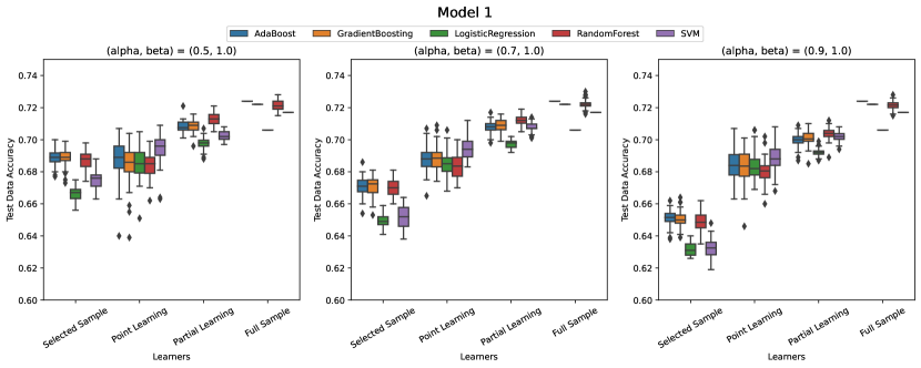
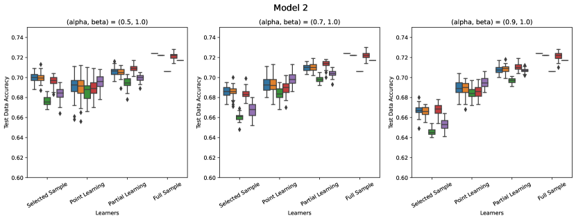
Figure 2: The testing accuracy of different methods with $\alpha=[0.5,0.7,0.9]$ and $\beta=1.0$ under Model 1 and Model 2 in eq. 6.1 respectively.

In this section, we evaluate the performance of our proposed algorithm in a semi-synthetic experiment based on the home loans dataset from FICO [2018]. This dataset consists of $10459$ observations of approved home loan applications. The dataset records whether the applicant repays the loan within $90$ days overdue, which we view as the true outcome $Y^{*}$, and various transaction information of the bank account. The dataset also includes a variable called ExternalRisk, which is a risk score assigned to each application by a proprietary algorithm. We consider ExternalRisk and all transaction features as the observed features $X$.

Synthetic selective labeling.

In this dataset the label of interest is fully observed, so we choose to synthetically create selective labels on top of the dataset. Specifically, we simulate $10$ decision-makers (e.g., bank officers who handle the loan applications) and randomly assign one to each case. We simulate the decision $D$ from a Bernoulli distribution with a success rate $p_{D}$ that depends on an “unobservable” variable $U$, the decision-maker identity $Z$, and the ExternalRisk variable (which serves as an algorithmic assistance to human decision-making). We blind the true outcome $Y^{*}$ for observations with $D=0$. Specifically, we construct $U$ as the residual from a random forest regression of $Y^{*}$ with respect to $X$ over the whole dataset, which is naturally dependent with $Y^{*}$. We then specify $p_{D}$ according to

Model 1: $$p_{D}=\beta\cdot\Big{(}\alpha\cdot\text{expit}\big{\{}U\big{\}}+(1-\alpha)\cdot\text{expit}\big{\{}(1+Z)\cdot\text{ExternalRisk}\big{\}}\Big{)},$$ (6.1)

Model 2: $$p_{D}=\beta\cdot\Big{(}\text{expit}\big{\{}\alpha\cdot U+(1-\alpha)\cdot(1+Z)\cdot\text{ExternalRisk}\big{\}}\Big{)}.$$

Here the $\operatorname{expit}$ function is given by $\operatorname{expit}(t)=1/(1+\exp(-t))$. The parameter $\alpha\in(0,1)$ controls the impact of $U$ on the labeling process and thus the degree of selection bias, and the parameter $\beta\in(0,1)$ further adjusts the overall label missingness. We can easily verify that the point-identification condition in eq. 3.2 holds under Model 1 but it does not hold under Model 2.

Methods and Evaluation.

We randomly split our data into training and and testing sets at a $7:3$ ratio. On the training set, we apply four types of different methods. The first two are our proposed method corresponding to the point identification and partial identification settings (“point learning” and “partial learning”) respectively.

The third and fourth are to run classification algorithms on the labeled subset only (“selected sample”) and the full training set (“full sample”). For each type of method, we try multiple different classification algorithms including AdaBoost, Gradient Boosting, Logistic Regression, Random Forest, and SVM. Our proposed method also need to estimate some unknown weight functions, which we implement by $K=5$ fold cross-fitted Gradient Boosting. All hyperparameters are chosen via $5$-fold cross-validation. See Appendix D for more details. We evaluate the classification accuracy of the resulting classifiers on the testing data.

Results and Discussions.

Figure 2 reports the testing accuracy of each method in $50$ replications of the experiment when $\beta=1$ and $\alpha\in\{0.5,0.7,0.9\}$. We observe that as the degree of selection bias $\alpha$ grows, the gains from using our proposed method relative to the “selected sample” baseline also grows, especially for the “partial learning” method. Interestingly, the “partial learning” method has better performance even under Model 1 when the point identification condition holds. This is perhaps because the “point learning” method requires estimating a conditional variance ratio, which is often difficult in practice. In contrast, the “partial learning” method only requires estimating conditional expectations and tends to be more stable. This illustrates the advantage of the “partial learning” method: it is robust to the failure of point-identification, and it can achieve more stable performance even when point-identification indeed holds. In Appendix D, we further report the results for $\beta\in\{0.5,0.25\}$ with more missing labels. These are more challenging settings so the performance of our method and the “selected sample” baseline all degrades, but our proposed methods (especially the “partial learning” method) still outperform the baseline.

7 Conclusion

In this paper, we study the evaluation and learning of a prediction rule with selective labels. We exploit a particular structure of heterogeneous decision-makers that arises in many applications. Specifically, we view the decision-maker assignment as an instrumental variable and rigorously analyze the identification of the full-population prediction risk. We propose a unified weighted formulation of the prediction risk (or its upper bound) when the risk is point-identified (or only partially identified). We develop a learning algorithm based on this formulation that can be efficiently implemented via standard machine learning packages, and empirically validate its benefit in numerical experiments.

Appendix A Supplement to Identification Analysis

A.1 Proofs for Section 3

Proof of Lemma 1.

To begin with, by the iterated law of expectation, we have

$$\mathbb{E}\big{[}\mathbb{I}\{Y^{*}\neq f(X)\}\big{]} =\mathbb{E}\Big{[}\mathbb{E}\big{[}\mathbb{I}\{Y^{*}\neq f(X)\}\mid X\big{]}\Big{]}$$

$$=\mathbb{E}\Big{[}\mathbb{P}(Y^{*}=1,f(X)=0\mid X)+\mathbb{P}(Y^{*}=0,f(X)=1\mid X)\Big{]}$$

$$=\mathbb{E}\Big{[}\mathbb{P}(Y^{*}=1\mid f(X)=0,X)\cdot\mathbb{P}(f(X)=0\mid X)\Big{]}$$

$$\quad+\mathbb{E}\Big{[}\mathbb{P}(Y^{*}=0\mid f(X)=1,X)\cdot\mathbb{P}(f(X)=1\mid X)\Big{]}.$$

It is essential to notice that

$$\mathbb{E}\Big{[}\mathbb{P}(Y^{*}=1\mid f(X)=0,X)\cdot\mathbb{P}(f(X)=0\mid X)\Big{]} =\mathbb{E}\Big{[}\mathbb{P}(Y^{*}=1\mid X)\cdot\mathbb{P}(f(X)=0\mid X)\Big{]}$$

$$=\mathbb{E}\Big{[}\mathbb{E}[Y^{*}\mid X]\cdot\mathbb{E}[1-f(X)\mid X]\Big{]}$$

$$=\mathbb{E}\Big{[}\mathbb{E}\big{[}\mu^{*}(X)\cdot(1-f(X))\mid X\big{]}\Big{]}$$

$$=\mathbb{E}\Big{[}\mu^{*}(X)\cdot(1-f(X))\Big{]}.$$

The first equality use the consistency of the probability conditioning on $X$, and the second equality holds because $Y^{*}$ and $f(X)$ are both binary random variables with support $\{0,1\}$. In a similar manner, we have

$$\mathbb{E}\Big{[}\mathbb{P}(Y^{*}=0\mid f(X)=1,X)\cdot\mathbb{P}(f(X)=1\mid X)\Big{]} =\mathbb{E}\Big{[}\mathbb{P}(Y^{*}=0\mid X)\cdot\mathbb{P}(f(X)=1\mid X)\Big{]}$$

$$=\mathbb{E}\Big{[}\mathbb{E}[1-Y^{*}\mid X]\cdot\mathbb{E}[f(X)\mid X]\Big{]}$$

$$=\mathbb{E}\Big{[}(1-\mu^{*}(X))\cdot f(X)\Big{]}.$$

Aggregating these together, we have

$$\mathbb{E}\big{[}\mathbb{I}(Y^{*}\neq f(X))\big{]}=\mathbb{E}\big{[}\mu^{*}(X)\big{]}+\mathbb{E}\big{[}(1-2\mu^{*}(X))\cdot f(X)\big{]}.$$

∎

Proof of Theorem 1.

We prove this result in two steps.

Step I. For any $z\in\mathcal{Z}$, the conditional expectation $\mathbb{E}[Y^{*}\mid X]$ could be expressed as

$$\mathbb{E}[Y^{*}\mid X] =\mathbb{E}\big{[}\mathbb{E}[Y^{*}\mid X,U]\mid X\big{]}$$

$$=\mathbb{E}\big{[}\mathbb{E}[Y^{*}\mid X,U,Z=z]\mid X\big{]}$$

$$=\mathbb{E}\big{[}\mathbb{E}[DY^{*}\mid X,U,Z=z]\mid X\big{]}+\mathbb{E}\big{[}\mathbb{E}[(1-D)Y^{*}\mid X,U,Z=z]\mid X\big{]}$$

$$=\mathbb{E}\big{[}\mathbb{E}[DY\mid X,U,Z=z]\mid X\big{]}+\mathbb{E}\big{[}\mathbb{E}[Y^{*}\mid X,U,Z=z]\cdot\mathbb{E}[(1-D)\mid X,U,Z=z]\mid X\big{]}$$

$$=\mathbb{E}\big{[}\mathbb{E}[DY\mid X,U,Z=z]\mid X,Z=z\big{]}+\mathbb{E}\big{[}\mathbb{E}[Y^{*}\mid X,U]\cdot\mathbb{E}[(1-D)\mid X,U,Z=z]\mid X\big{]}.$$

In the first equality, we apply the iterated law of expectation, and the IV independence is used in the second equality. In the fourth equality, we utilize the unconfoundedness and the last equality follows from IV independence again. Equivalently, we have

$$\mathbb{E}[Y^{*}\mid X]=\mathbb{E}[DY\mid X,Z=z]+\mathbb{E}\big{[}\mathbb{E}[Y^{*}\mid X,U]\cdot\mathbb{E}[(1-D)\mid X,U,Z=z]\mid X\big{]}.$$ (A.1)

By subtracting $\mathbb{E}[Y^{*}\mid X]$ on both sides of the equality, we have for any $z\in\mathcal{Z}$,

$$0=\mathbb{E}[DY\mid X,Z=z]-\mathbb{E}\big{[}\mathbb{E}[Y^{*}\mid X,U]\cdot\mathbb{E}[D\mid X,U,Z=z]\mid X\big{]}.$$

Multiplying the weight $z\cdot\mathbb{P}(Z=z\mid X)$ on both sides of equation above generates the following:

$$0=\mathbb{E}[zDY\mid X,Z=z]\cdot\mathbb{P}(Z=z\mid X)-\mathbb{E}\big{[}\mathbb{E}[Y^{*}\mid X,U]\cdot\mathbb{E}[zD\mid X,U,Z=z]\cdot\mathbb{P}(Z=z\mid X,U)\mid X\big{]}.$$

Here we using the fact that instrumental variable $Z$ is independent with $U$ given $X$ (Assumption 2) again. Taking the summation (or integral) over $\mathcal{Z}$ yields the following results:

$$0=\mathbb{E}[ZDY\mid X]-\mathbb{E}\big{[}\mathbb{E}[Y^{*}\mid X,U]\cdot\mathbb{E}[ZD\mid X,U]\mid X\big{]}.$$

Finally, observe that

$$\left\{\begin{aligned} &\mathbb{E}[ZDY\mid X]=\mathrm{Cov}(DY,Z\mid X)+\mathbb{E}[DY\mid X]\cdot\mathbb{E}[Z\mid X]\\ &\mathbb{E}[ZD\mid X,U]=\mathrm{Cov}(D,Z\mid X,U)+\mathbb{E}[D\mid X,U]\cdot\mathbb{E}[Z\mid X,U]\\ \end{aligned}\right.$$

we have

$$0 =\underbrace{\mathrm{Cov}(DY,Z\mid X)}_{\text{I}}+\underbrace{\mathbb{E}[DY^{*}\mid X]\cdot\mathbb{E}[Z\mid X]}_{\text{II}}-\underbrace{\mathbb{E}\big{[}\mathbb{E}[Y^{*}\mid X,U]\cdot\mathrm{Cov}(D,Z\mid X,U)\mid X\big{]}}_{\text{III}}$$ (A.2)

$$\quad-\underbrace{\mathbb{E}\big{[}\mathbb{E}[Y^{*}\mid X,U]\cdot\mathbb{E}[D\mid X,U]\cdot\mathbb{E}[Z\mid X,U]\mid X\big{]}}_{\text{IV}},$$

where here we use the fact that $\mathbb{E}[DY^{*}\mid X]=\mathbb{E}[DY\mid X]$. By the assumptions of unconfoundedness and IV independence again, we have

$$\mathbb{E}[Y^{*}\mid X,U]\cdot\mathbb{E}[D\mid X,U]\cdot\mathbb{E}[Z\mid X,U]=\mathbb{E}[DY^{*}\mid X,U]\cdot\mathbb{E}[Z\mid X].$$

Therefore the II and IV terms in eq. A.2 cancel out, which show us that

$$0=\mathrm{Cov}(DY,Z\mid X)-\mathbb{E}\big{[}\mathbb{E}[Y^{*}\mid X,U]\cdot\mathrm{Cov}(D,Z\mid X,U)\mid X\big{]}.$$ (A.3)

Step II. By assuming that

$$\mathrm{Cov}\big{(}\mathrm{Cov}(D,Z\mid X,U),\ \mathbb{E}[Y^{*}\mid X,U]\mid X\big{)}=0,$$

we have

$$\mathbb{E}\big{[}\mathbb{E}[Y^{*}\mid X,U]\cdot\mathrm{Cov}(D,Z\mid X,U)\mid X\big{]}=\mathbb{E}\big{[}\mathbb{E}[Y^{*}\mid X,U]\mid X\big{]}\cdot\mathbb{E}\big{[}\mathrm{Cov}(D,Z\mid X,U)\mid X\big{]}.$$

According to conditional covariance identity, we have

$$\mathrm{Cov}(D,Z\mid X) =\mathbb{E}\big{[}\mathrm{Cov}(D,Z\mid X,U)\mid X\big{]}+\mathbb{E}\big{[}\mathrm{Cov}(\mathbb{E}[D\mid X,U],\mathbb{E}[Z\mid X,U])\mid X\big{]}$$ (A.4)

$$=\mathbb{E}\big{[}\mathrm{Cov}(D,Z\mid X,U)\mid X\big{]}+\mathbb{E}\big{[}\mathrm{Cov}(\mathbb{E}[D\mid X,U],\mathbb{E}[Z\mid X])\mid X\big{]}$$

$$=\mathbb{E}\big{[}\mathrm{Cov}(D,Z\mid X,U)\mid X\big{]}.$$

Combining eq. A.4 with eq. A.3 leads us to the desired result, that is,

$$\mathbb{E}[Y^{*}\mid X]=\frac{\mathrm{Cov}(DY,Z\mid X)}{\mathrm{Cov}(D,Z\mid X)}:=r(X).$$

Substitute the result into risk function $\mathcal{R}_{\text{oracle}}(f)$ in (3.1) completes this proof.

∎

Proof of Proposition 1.

Notice that the conditional covariance $\mathrm{Cov}(D,Z\mid X,U)$ could be decomposed as

$$\mathrm{Cov}(D,Z\mid X,U)=\mathbb{E}[DZ\mid X,U]-\mathbb{E}[D\mid X,U]\cdot\mathbb{E}[Z\mid X,U]$$

$$= \sum_{j=1}^{m}\mathbb{E}[DZ\mid X,U,Z=j]\cdot\mathbb{P}(Z=j\mid X,U)-\mathbb{E}[D\mid X,U]\cdot\sum_{j=1}^{m}j\cdot\mathbb{P}(Z=j\mid X,U)$$

$$= \sum_{j=1}^{m}j\cdot\mathbb{E}[D\mid X,U,Z=j]\cdot\mathbb{P}(Z=j\mid X,U)$$

$$\quad-\sum_{k=1}^{m}\mathbb{E}[D\mid X,U,Z=k]\cdot\mathbb{P}(Z=k\mid X,U)\cdot\sum_{j=1}^{m}j\cdot\mathbb{P}(Z=j\mid X,U)$$

$$= \sum_{k=1}^{m}\sum_{j=1}^{m}j\cdot\mathbb{P}(Z=j\mid X,U)\cdot\mathbb{P}(Z=k\mid X,U)\cdot\big{[}\mathbb{E}[D\mid X,U,Z=j]-\mathbb{E}[D\mid X,U,Z=k]\big{]}.$$

Therefore, if

$$\mathrm{Cov}\big{(}\mathbb{E}[D\mid Z=j,X,U]-\mathbb{E}[D\mid Z=k,X,U],\ \mathbb{E}[Y^{*}\mid X,U]\mid X\big{)}=0,\quad\forall\ j,k\in[m]$$

almost surely, Theorem 1 is guaranteed by the decomposition above.

∎

Proof of Lemma 2.

According to (A.1), for any $z\in\mathcal{Z}$, the conditional expectation $\mathbb{E}[Y^{*}\mid X]$ could be expressed as

$$\mathbb{E}[Y^{*}\mid X]=\mathbb{E}[DY\mid X,Z=z]+\mathbb{E}\big{[}\mathbb{E}[Y^{*}\mid X,U]\cdot\mathbb{E}[(1-D)\mid X,U,Z=z]\mid X\big{]}.$$

Since this formula holds for every $z\in\mathcal{Z}$, we must have

$$\mathbb{E}[Y^{*}\mid X] =\max_{z\in\mathcal{Z}}\Big{\{}\mathbb{E}[DY\mid X,Z=z]+\mathbb{E}\big{[}\mathbb{E}[Y^{*}\mid X,U]\cdot\mathbb{E}[(1-D)\mid X,U,Z=z]\mid X\big{]}\Big{\}}$$

$$\mathbb{E}[Y^{*}\mid X] =\min_{z\in\mathcal{Z}}\Big{\{}\mathbb{E}[DY\mid X,Z=z]+\mathbb{E}\big{[}\mathbb{E}[Y^{*}\mid X,U]\cdot\mathbb{E}[(1-D)\mid X,U,Z=z]\mid X\big{]}\Big{\}}.$$

Without loss of generality, we assume $\mathbb{E}[(1-D)\mid X,U,Z=z]\geq 0$. As we have assumed that $\mathbb{E}[Y^{*}\mid X,U]\in[\alpha(X),\beta(X)]$ in Assumption 3, we then have

$$\mathbb{E}[Y^{*}\mid X] \geq\max_{z\in\mathcal{Z}}\Big{\{}\mathbb{E}[DY\mid X,Z=z]+\alpha(X)\cdot\mathbb{E}\big{[}\mathbb{E}[(1-D)\mid X,U,Z=z]\mid X,Z=z\big{]}\Big{\}}$$ (A.5)

$$=\max_{z\in\mathcal{Z}}\Big{\{}\mathbb{E}[DY\mid X,Z=z]+\alpha(X)\cdot\mathbb{E}[(1-D)\mid X,Z=z]\Big{\}}.$$

If $\alpha(X)$ is a sharp lower bound for $\mathbb{E}[Y^{*}\mid X,U]$, the lower bound (eq. A.5) is also sharp for $\mathbb{E}[Y^{*}\mid X]$. Similarly, we have

$$\mathbb{E}[Y^{*}\mid X] \leq\min_{z\in\mathcal{Z}}\Big{\{}\mathbb{E}[DY\mid X,Z=z]+\beta(X)\cdot\mathbb{E}\big{[}\mathbb{E}[(1-D)\mid X,U,Z=z]\mid X,Z=z\big{]}\Big{\}}$$

$$=\min_{z\in\mathcal{Z}}\Big{\{}\mathbb{E}[DY\mid X,Z=z]+\beta(X)\cdot\mathbb{E}[(1-D)\mid X,Z=z]\Big{\}}.$$

Combining the results above, we have

$$\max_{z\in\mathcal{Z}}\ \Big{\{}\mathbb{E}[DY\mid X,Z=z]+\alpha(X)\cdot\big{(}1-\mathbb{E}[D\mid X,Z=z]\big{)}\Big{\}}$$

$$\qquad\qquad\qquad\qquad\leq\mathbb{E}[Y\mid X]\leq$$

$$\min_{z\in\mathcal{Z}}\ \Big{\{}\mathbb{E}[DY\mid X,Z=z]+\beta(X)\cdot\big{(}1-\mathbb{E}[D\mid X,Z=z]\big{)}\Big{\}}.$$

∎

Proof of Theorem 2.

For any $\mu^{\prime}(X)\in[l(X),u(X)]$, we have

$$(1/2-\mu^{\prime}(X))f(X)\leq\max_{\mu(X)\in[l(X),u(X)]}\left\{(1-2\mu(X))f(X)\right\}.$$

The inequality above still holds when we take expectation on both sides, which suggests that $\mathcal{R}(f)\leq\overline{\mathcal{R}}(f)$. We can show that $\mathcal{R}(f)\geq\underline{\mathcal{R}}(f)$ in a similar way.

∎

A.2 Balke and Pearl’s Bound

Balke and Pearl [1994] provides partial identification bounds for the average treatment effect of a binary treatment with a binary instrumental variable. In this section, we adapt their bound to our setting with partially observed labels and a binary IV (i.e., the assignment to one of two decision-makers). Under Assumption 2, we have following decomposition of joint probability distribution of $(Y,D,Z,U)$

$$\mathbb{P}(Y,D,Z,U)=\mathbb{P}(Y\mid D,U)\cdot\mathbb{P}(D\mid Z,U)\cdot\mathbb{P}(Z)\cdot\mathbb{P}(U).$$ (A.6)

Here we omit the observed covariates $X$ for simplicity, or alternatively, all distributions can be considered as implicitly conditioning on $X$. Now we define three response functions which characterize the values of $Z$, $D(0),D(1)$, and $Y^{*}$:

$$r_{Z}=\left\{\begin{aligned} &0\ &\text{if}\ Z=0\\ &1\ &\text{if}\ Z=1\\ \end{aligned}\right.,\quad r_{D}=\left\{\begin{aligned} &0\quad&\text{if}\quad D(0)=0\ \text{and}\ D(1)=0\\ &1\quad&\text{if}\quad D(0)=0\ \text{and}\ D(1)=1\\ &2\quad&\text{if}\quad D(0)=1\ \text{and}\ D(1)=0\\ &3\quad&\text{if}\quad D(0)=1\ \text{and}\ D(1)=1\\ \end{aligned}\right.,\quad r_{Y}=\left\{\begin{aligned} &0\ &\text{if}\quad Y^{*}=0\\ &1\ &\text{if}\quad Y^{*}=1\\ \end{aligned}\right..$$

Next, we specify the joint distribution of unobservable variables $r_{D}$ and $r_{Y}$ as follows:

$$q_{kj}=\mathbb{P}(r_{D}=k,r_{Y}=j)\quad\forall\ k\in\{0,1,2,3\},\ j\in\{0,1\},$$

which satisfies the constraint $\sum_{k=0}^{3}(q_{k0}+q_{k1})=1$. Then the target mean parameter of the true outcome can be written as a linear combinations of the $q$’s. Moreover, we note that the observable distribution $\mathbb{P}(Y,D\mid Z)$ is fully specified by the following six variables

$$p_{na,0}=\mathbb{P}(D=0\mid Z=0)\qquad p_{na,1}=\mathbb{P}(D=0\mid Z=1)$$

$$p_{01,0}=\mathbb{P}(Y=0,D=1\mid Z=0)\qquad p_{01,1}=\mathbb{P}(Y=0,D=1\mid Z=1)$$

$$p_{11,0}=\mathbb{P}(Y=1,D=1\mid Z=0)\qquad p_{11,1}=\mathbb{P}(Y=1,D=1\mid Z=1),$$

with constraints $p_{11,0}+p_{01,0}+p_{na,0}=1$ and $p_{11,1}+p_{01,1}+p_{na,1}=1$. We also have the following relation between $p$’s and $q$’s:

$$\begin{aligned} p_{na,0}&=q_{00}+q_{01}+q_{10}+q_{11}\\ p_{01,0}&=q_{20}+q_{30}\\ p_{11,0}&=q_{21}+q_{31}\\ \end{aligned}\qquad\begin{aligned} p_{na,1}&=q_{00}+q_{01}+q_{20}+q_{21}\\ p_{01,1}&=q_{10}+q_{30}\\ p_{11,1}&=q_{11}+q_{31}.\\ \end{aligned}$$

Therefore, we have $p=Pq$ where $p=(p_{na,0},\dots,p_{11,1})$, $q=(q_{00},\dots,q_{31})$, and

$$P=\begin{bmatrix}1&1&0&0&1&1&0&0\\ 0&0&1&1&0&0&0&0\\ 0&0&0&0&0&0&1&1\\ 1&0&1&0&1&0&1&0\\ 0&1&0&1&0&0&0&0\\ 0&0&0&0&0&1&0&1\\ \end{bmatrix}.$$

Then the lower bound on $\mathbb{E}\left[{Y^{*}}\right]$ can be written as the optimal value of the following linear programming problem

$$\begin{aligned} \operatorname*{\mathrm{minimize}}\quad&q_{01}+q_{11}+q_{21}+q_{31}\\ \text{subject to}\quad&\sum_{k=0}^{3}\sum_{j=0}^{1}q_{kj}=1\\ &Pq=p\\ &q_{kj}\geq 0\quad k\in\{0,1,2,3\},\ j\in\{0,1\}.\\ \end{aligned}.$$ (A.7)

Similarly, the upper bound on $\mathbb{E}\left[{Y^{*}}\right]$ can be written as the optimal value of the following optimization problem:

$$\operatorname*{\mathrm{maximize}} q_{01}+q_{11}+q_{21}+q_{31}$$ (A.8)

subject to $$\sum_{k=0}^{3}\sum_{j=0}^{1}q_{kj}=1$$

$$Pq=p$$

$$q_{kj}\geq 0\quad k\in\{0,1,2,3\},\ j\in\{0,1\}.$$

In fact, by simply comparing the variables in the objective function $\mathbb{E}[Y^{*}]=q_{01}+q_{11}+q_{21}+q_{31}$ and those in constraints, one could find that

$$p_{11,0}=q_{21}+q_{31}\leq\mathbb{E}[Y^{*}]$$

$$p_{11,1}=q_{11}+q_{31}\leq\mathbb{E}[Y^{*}]$$

$$p_{11,0}+p_{na,0}=q_{00}+q_{10}+q_{01}+q_{11}+q_{21}+q_{31}\geq\mathbb{E}[Y^{*}]$$

$$p_{11,1}+p_{na,1}=q_{00}+q_{20}+q_{01}+q_{11}+q_{21}+q_{31}\geq\mathbb{E}[Y^{*}].$$

If we let

$$L =\max\{p_{11,0},p_{11,1}\}=\max_{z\in\{0,1\}}\ \Big{\{}\mathbb{P}(Y=1,D=1\mid Z=z)\Big{\}}$$ (A.9)

$$U =\min\{p_{11,0}+p_{na,0},p_{11,1}+p_{na,1}\}=\min_{z\in\{0,1\}}\ \Big{\{}\mathbb{P}(Y=1,D=1\mid Z=z)+\mathbb{P}(D=0\mid Z=z)\Big{\}}.$$

We then have the following partial bounds of $\mathbb{E}[Y\mid X]$.

$$L\ \leq\ \mathbb{E}[Y^{*}]\ \leq\ U.$$

According to Balke and Pearl [1994], the bounds above are tight for $\mathbb{E}[Y^{*}]$. We note that if we condition on $X$ in these bounds, then the corresponding bound on $\mathbb{E}\left[{Y^{*}\mid X}\right]$ coincide with the bounds in Lemma 2 specialized to a binary instrument.

Appendix B Proofs for Section 4

Proof of Lemma 3.

Recall that $\mathcal{R}_{\text{oracle}}(f)=\mathbb{E}[\mu^{*}(X)+(1-2\mu^{*}(X))f(X)]$ where $\mu^{*}(X):=\mathbb{E}[Y^{*}\mid X]$. Suppose there is a real-valued function $h$ on $\mathcal{X}$ such that for each $f$, we have $f(X)=(\operatorname*{\mathrm{sgn}}[h(X)]+1)/2$. Let $\eta^{*}(X)=\mu^{*}(X)-1/2$, we have,

$$\mathcal{R}_{\text{oracle}}(f) =\mathbb{E}\left[\mu^{*}(X)+(1-2\mu^{*}(X))\left(\frac{\operatorname*{\mathrm{sgn}}[h(X)]+1}{2}\right)\right]$$

$$=\frac{1}{2}+\mathbb{E}\left[\left(\frac{1}{2}-\mu^{*}(X)\right)\operatorname*{\mathrm{sgn}}[h(X)]\right]$$

$$=\frac{1}{2}+\mathbb{E}\Big{[}\left(-\eta^{*}(X)\right)\operatorname*{\mathrm{sgn}}[h(X)]\Big{]}:=\mathcal{R}_{\text{oracle}}(h).$$

Here we redefine the oracle risk function $\mathcal{R}_{\text{oracle}}(h)$ with respect to $h$, which can be further decomposed into

$$\mathcal{R}_{\text{oracle}}(h) =\frac{1}{2}+\mathbb{E}\Big{[}(-\eta^{*}(X))\operatorname*{\mathrm{sgn}}[h(X)]\Big{]}$$

$$=\frac{1}{2}+\mathbb{E}\Big{[}|\eta^{*}(X)|\cdot\operatorname*{\mathrm{sgn}}[-\eta^{*}(X)]\operatorname*{\mathrm{sgn}}[h(X)]\Big{]}$$

$$=\frac{1}{2}+\mathbb{E}\Big{[}|\eta^{*}(X)|\cdot\Big{(}2\mathbb{I}\{\operatorname*{\mathrm{sgn}}[\eta^{*}(X)]\neq\operatorname*{\mathrm{sgn}}[h(X)]\}-1\Big{)}\Big{]}$$

$$=\frac{1}{2}-\mathbb{E}[|\eta^{*}(X)|]+2\mathbb{E}\Big{[}|\eta^{*}(X)|\cdot\mathbb{I}\{\operatorname*{\mathrm{sgn}}[\eta^{*}(X)]\neq\operatorname*{\mathrm{sgn}}[h(X)]\}\Big{]}$$

$$:=C_{0}+\mathcal{R}(h).$$

Here we let $C_{0}=1/2-\mathbb{E}[|\eta^{*}(X)|]$ and $\mathcal{R}(h):=\mathbb{E}\Big{[}|\eta^{*}(X)|\cdot\mathbb{I}\{\operatorname*{\mathrm{sgn}}[\eta^{*}(X)]\neq\operatorname*{\mathrm{sgn}}[h(X)]\}\Big{]}$ and the constant term $2$ is omitted as it does not affect the optimization over $h$. Therefore, in the sequel, we only consider optimizing the risk function $\mathcal{R}(h)$ instead.

∎

Proof of Theorem 3.

Recall from Lemma 3 that $\mathcal{R}(h)=\mathbb{E}[|\eta^{*}(X)|\cdot\mathbb{I}\{\operatorname*{\mathrm{sgn}}[\eta^{*}(X)]\neq\operatorname*{\mathrm{sgn}}[h(X)]\}]$ where $\eta^{*}(X)=\mu^{*}(X)-1/2$.

Under the case of point identification, the conditional mean function $\mu^{*}(X)$ is identified as $r(X)=\frac{\mathrm{Cov}(DY,Z\mid X)}{\mathrm{Cov}(D,Y\mid X)}$. We then have $w_{\operatorname{point}}(X):=r(X)-1/2=\eta^{*}(X)$. In this case, we define the risk function origins from $\mathcal{R}(h)$ as

$$\mathcal{R}_{\operatorname{point}}(h):=\mathbb{E}\Big{[}|w_{\operatorname{point}}|\cdot\mathbb{I}\{\operatorname*{\mathrm{sgn}}[w_{\operatorname{point}}(X)]\neq\operatorname*{\mathrm{sgn}}[h(X)]\}\Big{]}.$$ (B.1)

Under the case of partial identification, we have $\mu^{*}(X)\in[l(X),u(X)]$. Let $\tilde{l}(X)=l(X)-1/2$ and $\tilde{u}(X)=u(X)-1/2$, we then have $\eta^{*}(X)\in[\tilde{l}(X),\tilde{u}(X)]$. In this sense, we define partial risk from $\mathcal{R}(h)$ as

$$\mathcal{R}_{\operatorname{partial}}(h):=\mathbb{E}\left[\max_{\eta(X)\in[\tilde{l}(X),\tilde{u}(X)]}|\eta(X)|\cdot\mathbb{I}\{\operatorname*{\mathrm{sgn}}(\eta(X))\neq\operatorname*{\mathrm{sgn}}(h(X))\}\right],$$ (B.2)

which can be further written as

$$\mathcal{R}_{\operatorname{partial}}(h) =\mathbb{E}\left[\max_{\eta(X)\in[\tilde{l}(X),\tilde{u}(X)]}|\eta(X)|\cdot\mathbb{I}\{\operatorname*{\mathrm{sgn}}[\eta(X)]\neq\operatorname*{\mathrm{sgn}}[h(X)]\}\right]$$

$$=\mathbb{E}\left[\mathbb{E}\left[\max_{\eta(X)\in[\tilde{l}(X),\tilde{u}(X)]}|\eta(X)|\cdot\mathbb{I}\{\operatorname*{\mathrm{sgn}}[\eta(X)]\neq\operatorname*{\mathrm{sgn}}[h(X)]\}\mid\tilde{l}(X),\tilde{u}(X)\right]\right]$$

$$=\mathbb{E}\Big{[}|\tilde{u}(X)|\cdot\mathbb{I}\{1\neq\operatorname*{\mathrm{sgn}}[(X)]\}\cdot\mathbb{I}\{\tilde{l}(X)>0\}\Big{]}+\mathbb{E}\Big{[}|\tilde{l}(X)|\cdot\mathbb{I}\{-1\neq\operatorname*{\mathrm{sgn}}[h(X)]\}\cdot\mathbb{I}\{\tilde{u}(X)<0\}\Big{]}$$

$$\quad+\mathbb{E}\Big{[}\max\big{(}|\tilde{u}(X)|\cdot\mathbb{I}\{1\neq\operatorname*{\mathrm{sgn}}[h(X)]\},\ |\tilde{l}(X)|\cdot\mathbb{I}\{-1\neq\operatorname*{\mathrm{sgn}}[h(X)]\}\big{)}\cdot\mathbb{I}\{0\in[\tilde{l}(X),\tilde{u}(X)]\}\Big{]}$$

$$=\mathbb{E}\Big{[}|\tilde{u}(X)|\cdot\mathbb{I}\{1\neq\operatorname*{\mathrm{sgn}}[h(X)]\}\cdot\mathbb{I}\{\tilde{l}(X)>0\}\Big{]}+\mathbb{E}\Big{[}|\tilde{l}(X)|\cdot\mathbb{I}\{-1\neq\operatorname*{\mathrm{sgn}}[h(X)]\}\cdot\mathbb{I}\{\tilde{u}(X)<0\}\Big{]}$$

$$\quad+\mathbb{E}\Big{[}|\tilde{u}(X)|\cdot\mathbb{I}\{1\neq\operatorname*{\mathrm{sgn}}[h(X)]\}\cdot\mathbb{I}\{0\in[\tilde{l}(X),\tilde{u}(X)]\}\Big{]}$$

$$\quad+\mathbb{E}\Big{[}|\tilde{l}(X)|\cdot\mathbb{I}\{-1\neq\operatorname*{\mathrm{sgn}}[h(X)]\}\cdot\mathbb{I}\{0\in[\tilde{l}(X),\tilde{u}(X)]\}\Big{]}$$

$$=\mathbb{E}\Big{[}|\tilde{u}(X)|\cdot\mathbb{I}\{1\neq\operatorname*{\mathrm{sgn}}[h(X)]\}\cdot\mathbb{I}\{\tilde{u}(X)>0\}\Big{]}+\mathbb{E}\Big{[}|\tilde{l}(X)|\cdot\mathbb{I}\{-1\neq\operatorname*{\mathrm{sgn}}[h(X)]\}\cdot\mathbb{I}\{\tilde{l}(X)<0\}\Big{]}$$

$$=\mathbb{E}\Big{[}|\tilde{u}(X)|\cdot\mathbb{I}\{1\neq\operatorname*{\mathrm{sgn}}[h(X)]\}\cdot\mathbb{I}\{\tilde{u}(X)>0\}\Big{]}+\mathbb{E}\Big{[}|\tilde{l}(X)|\cdot\big{(}1-\mathbb{I}\{1\neq\operatorname*{\mathrm{sgn}}[h(X)]\}\big{)}\cdot\mathbb{I}\{\tilde{l}(X)<0\}\Big{]}$$

$$=\mathbb{E}\Big{[}|\tilde{l}(X)|\cdot\mathbb{I}\{\tilde{l}(X)<0\}\Big{]}+\mathbb{E}\Big{[}\big{(}|\tilde{u}(X)|\cdot\mathbb{I}\{\tilde{u}(X)>0\}-|\tilde{l}(X)|\cdot\mathbb{I}\{\tilde{l}(X)<0\}\big{)}\cdot\mathbb{I}\{1\neq\operatorname*{\mathrm{sgn}}[h(X)]\}\Big{]}.$$

Let $w_{\operatorname{partial}}(X)=|\tilde{u}(X)|\cdot\mathbb{I}\{\tilde{u}(X)>0\}-|\tilde{l}(X)|\cdot\mathbb{I}\{\tilde{l}(X)<0\}$, we have

$$\mathcal{R}_{\operatorname{partial}}(h) =\underbrace{\mathbb{E}\Big{[}|\tilde{l}(X)|\cdot\mathbb{I}\{\tilde{l}(X)<0\}\Big{]}}_{(\cdots)}+\mathbb{E}[w_{\operatorname{partial}}(X)\cdot\mathbb{I}\{1\neq\operatorname*{\mathrm{sgn}}[h(X)]\}]$$

$$=(\dots)+\mathbb{E}\left[w_{\operatorname{partial}}(X)\cdot\frac{1-\operatorname*{\mathrm{sgn}}(h(X))}{2}\right]$$

$$=(\dots)+\frac{1}{2}\mathbb{E}\big{[}w_{\operatorname{partial}}(X)\big{]}+\frac{1}{2}\mathbb{E}\big{[}-w_{\operatorname{partial}}(X)\cdot\operatorname*{\mathrm{sgn}}[h(X)]\big{]}$$

$$=(\dots)+\frac{1}{2}\mathbb{E}\big{[}w_{\operatorname{partial}}(X)\big{]}+\frac{1}{2}\mathbb{E}\big{[}|w_{\operatorname{partial}}(X)|\cdot\operatorname*{\mathrm{sgn}}[-w_{\operatorname{partial}}(X)]\cdot\operatorname*{\mathrm{sgn}}[h(X)]\big{]}$$

$$=(\dots)+\frac{1}{2}\mathbb{E}\big{[}w_{\operatorname{partial}}(X)\big{]}+\frac{1}{2}\mathbb{E}\Big{[}|w_{\operatorname{partial}}(X)|\cdot\Big{(}2\mathbb{I}\{\operatorname*{\mathrm{sgn}}[w_{\operatorname{partial}}(X)]\neq\operatorname*{\mathrm{sgn}}[h(X)]\}-1\Big{)}\Big{]}$$

$$=(\cdots)+\mathbb{E}\Big{[}|w_{\operatorname{partial}}(X)|\cdot\mathbb{I}\{\operatorname*{\mathrm{sgn}}[w_{\operatorname{partial}}(X)]\neq\operatorname*{\mathrm{sgn}}[h(X)]\}\Big{]}.$$

Since the term $(\cdots)$ does not affect the optimization over $h$, we may drop it in the sequel. Therefore, with slight abuse of notation, we define the risk function under partial identification as

$$\mathcal{R}_{\operatorname{partial}}:=\mathbb{E}\Big{[}|w_{\operatorname{partial}}(X)|\cdot\mathbb{I}\{\operatorname*{\mathrm{sgn}}[w_{\operatorname{partial}}(X)]\neq\operatorname*{\mathrm{sgn}}(h(X))\}\Big{]},$$ (B.3)

where $w_{\operatorname{partial}}(X)=|\tilde{u}(X)|\cdot\mathbb{I}\{\tilde{u}(X)>0\}-|\tilde{l}(X)|\cdot\mathbb{I}\{\tilde{l}(X)<0\}=\max(u(X)-1/2,0)+\min(l(X)-1/2,0)$.

Overall, the expected risk function under point and partial identification can be written in an unified form as

$$\mathcal{R}\left(h;w\right)=\mathbb{E}\left[{\left|w(X)\right|\mathbb{I}\{\operatorname*{\mathrm{sgn}}[w(X)]\neq\operatorname*{\mathrm{sgn}}[h(X)]\}}\right]$$

with $w_{\operatorname{point}}(X)=r(X)-1/2$ and $w_{\operatorname{partial}}(X)=\max(u(X)-1/2,0)+\min(l(X)-1/2,0)$.

∎

Appendix C Proofs for Section 5

C.1 Decomposition of Excess Risk

In this subsection, we will prove Lemma 4 in two steps. We first show that the excess risk $\mathcal{R}_{M}(\hat{h})-\inf_{h}\mathcal{R}_{M}(h)$ is boundned by the excess $\Phi$-risk $\mathcal{R}_{\Phi}(\hat{h};w_{M})-\min_{h}\mathcal{R}_{\Phi}(h;w_{M})$ with respect to Hinge loss, logistic loss and exponential loss for $M\in\{\operatorname{point},\operatorname{partial}\}$. We then complete the proof of Lemma 4 by showing that the excess $\Phi$-risk can be expressed in two parts.

Lemma 6 (Bounded Excess Risk).

Denote $\mathcal{R}_{M}^{*}=\inf_{h}\mathcal{R}_{M}(h)$ and $\mathcal{R}_{\Phi}^{*}=\inf_{h}\mathcal{R}_{\Phi}(h;w_{M})$. For any measurable function $h$ and $M\in\{\operatorname{point},\operatorname{partial}\}$, the excess risk with respect to $h$ is controlled by the excess $\Phi$-risk:

$$\mathcal{R}_{M}(h)-\mathcal{R}_{M}^{*}\leq\mathcal{R}_{\Phi}(h;w_{M})-\mathcal{R}_{\Phi}^{*}.$$

Proof of Lemma 6.

Let $h^{*}=\operatorname{arg}\min_{h}\mathcal{R}_{M}(h)$ be the Bayes optimal function which minimizes the expected risk $\mathcal{R}_{M}(h)$. For both $M\in\{\operatorname{point},\operatorname{partial}\}$, the excess risk with respect to measurable function $h$ can be written into

$$\mathcal{R}_{M}(h)-\mathcal{R}_{M}^{*} =\mathbb{E}\Big{[}|w_{M}(X)|\cdot\Big{(}\mathbb{I}\big{\{}\operatorname*{\mathrm{sgn}}[w_{M}(X)]\neq\operatorname*{\mathrm{sgn}}[h(X)]\big{\}}-\mathbb{I}\big{\{}\operatorname*{\mathrm{sgn}}[w_{M}(X)]\neq\operatorname*{\mathrm{sgn}}[h^{*}(X)]\big{\}}\Big{)}\Big{]}$$

$$=\mathbb{E}\Big{[}|w_{M}(X)|\cdot\mathbb{I}\big{\{}\operatorname*{\mathrm{sgn}}[h^{*}(X)]\neq\operatorname*{\mathrm{sgn}}[h(X)]\big{\}}\Big{]}.$$

Here we use the fact that the Bayes optimal function $h^{*}(X)$ should have the same sign as weight function $w(X)$.

Recall from (4.1) that the $\Phi$-risk is defined as $\mathcal{R}_{\Phi}(h;w)=\mathbb{E}[|w(X)|\cdot\Phi\left(\operatorname*{\mathrm{sgn}}[w(X)]\cdot h(X)\right)]$ and consider the surrogate loss functions:

$$\begin{aligned} &\text{Hinge loss}:&&\Phi(\alpha)=\max\{1-\alpha,0\}\\ &\text{logistic loss}:&&\Phi(\alpha)=\log(1+e^{-\alpha})\\ &\text{exponential loss}:&&\Phi(\alpha)=e^{-\alpha}\\ \end{aligned}.$$

Notice that for any $\Phi\in\{\operatorname{Hinge},\operatorname{logistic},\operatorname{exponential}\}$, the surrogate loss $\Phi(\alpha)$ is lower-bounded (in fact, $\inf_{\alpha}\Phi(\alpha)=0$), then we have $\inf_{\alpha}\mathbb{E}[\Phi(\alpha(X))]=\mathbb{E}[\inf_{\alpha}\Phi(\alpha(X))]$. Hence, for any given $w(X)$, the Bayes risk $\mathcal{R}_{\Phi}^{*}$ can be formalized as

$$\mathcal{R}_{\Phi}^{*}=\inf_{h}\mathbb{E}\Big{[}|w(X)|\cdot\Phi\big{(}\operatorname*{\mathrm{sgn}}[w(X)]\cdot h(X)\big{)}\Big{]}=\mathbb{E}\Big{[}\inf_{h}|w(X)|\cdot\Phi\big{(}\operatorname*{\mathrm{sgn}}[w(X)]\cdot h(X)\big{)}\Big{]},$$

which suggests that the excess $\Phi$-risk $\mathcal{R}_{\Phi}(h)-\mathcal{R}_{\Phi}^{*}$ can be written as the expectation of

$$|w(X)|\cdot\left[\mathbb{I}\{w(X)\geq 0\}\cdot\Big{(}\Phi(h(X))-\inf_{\alpha}\Phi(\alpha(X))\Big{)}+\mathbb{I}\{w(X)<0\}\cdot\Big{(}\Phi(-h(X))-\inf_{\alpha}\Phi(-\alpha(X))\Big{)}\right].$$

In the following contents, we compare the value of $\mathcal{R}_{M}(h)-\mathcal{R}_{M}^{*}$ and $\mathcal{R}_{\Phi}(h)-\mathcal{R}_{\Phi}^{*}$ by considering all possible value of $(w(X),h(X))$ for any fixed $X=x$.

• Consider the case when $w(x)\geq 0$, we have $\operatorname*{\mathrm{sgn}}[h^{*}(x)]=\operatorname*{\mathrm{sgn}}[w(x)]=+1$ and

  $$\mathbb{I}\big{\{}\operatorname*{\mathrm{sgn}}[h^{*}(x)]\neq\operatorname*{\mathrm{sgn}}[h(x)]\big{\}}=\mathbb{I}\big{\{}1\neq\operatorname*{\mathrm{sgn}}[h(x)]\big{\}}.$$

  Meanwhile, for any $\Phi\in\{\operatorname{Hinge},\operatorname{logistic},\operatorname{exponential}\}$, we have $\inf_{\alpha}\Phi(\alpha(x))=0$ and

  $$\Phi\big{(}h(x)\big{)}-\inf_{\alpha}\Phi\big{(}\alpha(x)\big{)}=\Phi(h(x))-0.$$

  • If $h(x)\geq 0$, then $\Phi(h(x))\geq 0$ holds for any $\Phi\in\{\operatorname{Hinge},\operatorname{logistic},\operatorname{exponential}\}$:

    $$\begin{aligned} \Phi_{\operatorname{Hinge}}\big{(}h(x)\big{)}&=(1-|h(x)|)^{+}\geq 0\\ \Phi_{\operatorname{logistic}}\big{(}h(x)\big{)}&=\log_{2}(1+e^{-|h(x)|})\geq 0\\ \Phi_{\operatorname{exponential}}\big{(}h(x)\big{)}&=e^{-|h(x)|}\geq 0\\ \end{aligned}.$$

    Therefore, we have

    $$\Phi\big{(}h(x)\big{)}-\inf_{\alpha}\Phi\big{(}\alpha(x)\big{)}\geq 0=\mathbb{I}\big{\{}1\neq\operatorname*{\mathrm{sgn}}[h(x)]\big{\}}.$$

  • If $h(x)<0$, then $\Phi(h(x))\geq 1$ holds for any $\Phi\in\{\operatorname{Hinge},\operatorname{logistic},\operatorname{exponential}\}$:

    $$\begin{aligned} \Phi_{\text{Hinge}}\big{(}h(x)\big{)}&=(1+|h(x)|)^{+}\geq 1\\ \Phi_{\text{logistic}}\big{(}h(x)\big{)}&=\log_{2}(1+e^{|h(x)|})\geq\log_{2}(1+e^{0})=1\\ \Phi_{\text{exponential}}\big{(}h(x)\big{)}&=e^{|h(x)|}\geq e^{0}=1\\ \end{aligned}.$$

    Therefore, we have

    $$\Phi\big{(}h(x)\big{)}-\inf_{\alpha}\Phi\big{(}\alpha(x)\big{)}\geq 1=\mathbb{I}\big{\{}1\neq\operatorname*{\mathrm{sgn}}[h(x)]\big{\}}.$$

• We can do the similar analysis when $w(x)<0$ and obtain the same conclusion that

  $$\Phi\big{(}h(x))-\inf_{\alpha}\Phi\big{(}\alpha(x)\big{)}\geq\mathbb{I}\{\operatorname*{\mathrm{sgn}}[h^{*}(x)]\neq h(x)\}.$$

Finally, by multiplying the common weight $|w(X)|$ and taking the expectation over $X$, we conclude that

$$\mathcal{R}_{\Phi}(h;w_{M})-\mathcal{R}_{\Phi}^{*}\geq\mathcal{R}_{M}(h)-\mathcal{R}_{M}^{*}.$$

Therefore, when the excess $\Phi$-risk is minimized, the original excess risk also attains its minimum.

∎

We are now ready to give the proof of Lemma 4.

Proof of Lemma 4.

Notice that the excess $\Phi$-risk defined in Lemma 6 can always be decomposed into

$$\mathcal{R}_{\Phi}(\hat{h};w_{M})-\inf_{h}\mathcal{R}_{\Phi}(h;w_{M})=\mathcal{R}_{\Phi}(\hat{h};w_{M})-\inf_{h\in\mathcal{H}}\mathcal{R}_{\Phi}(h;w_{M})+\inf_{h\in\mathcal{H}}\mathcal{R}_{\Phi}(h;w_{M})-\inf_{h}\mathcal{R}_{\Phi}(h;w_{M}).$$ (C.1)

Here we explicitly write the risk function $\mathcal{R}_{\Phi}$ in terms of hypothesis function $h$ as well as the weight function $w_{M}$ to emphasize the role of weight function $w(\cdot)$ in the risk function.

Finally, Combining the result of Lemma 6 with eq. C.1, we complete the proof of Lemma 4.

∎

C.2 Decomposition of Estimation Error

In this part, we further prove Lemma 5.

Proof of Lemma 5.

Let $h_{\Phi}^{*}=\operatorname{arg}\min_{h}\mathcal{R}_{\Phi}(h;w_{M})$ be the Bayes optimal minimiser of expected $\Phi$-risk, while denote $h_{\Phi,\mathcal{H}}^{*}\in\operatorname{arg}\min_{h\in\mathcal{H}}\mathcal{R}_{\Phi}(h;w_{M})$ be the best-in-class minimiser of expected $\Phi$-risk. We can now write the estimation error $\mathcal{E}(\mathcal{H})$ as

$$\mathcal{E}(\mathcal{H}) =\mathcal{R}_{\Phi}(\hat{h};w_{M})-\inf_{h\in\mathcal{H}}\mathcal{R}_{\Phi}(h;w_{M})=\mathcal{R}_{\Phi}(\hat{h};w_{M})-\mathcal{R}_{\Phi}(h_{\Phi,\mathcal{H}}^{*};w_{M})$$ (C.2)

$$=\underbrace{\Big{[}\mathcal{R}_{\Phi}(\hat{h};w_{M})-\mathcal{R}_{\Phi}(h_{\Phi}^{*};w_{M})\Big{]}}_{\text{Part I}}+\underbrace{\Big{[}\mathcal{R}_{\Phi}(h_{\Phi}^{*};w_{M})-\mathcal{R}_{\Phi}(h_{\Phi,\mathcal{H}}^{*};w_{M})\Big{]}}_{\text{Part II}}.$$

Note that $h_{\Phi}^{*}$ is the global optimal of expected $\Phi$-risk, we have $\text{Part II}\leq 0$. Before we go for Part I, we define

$$\overline{\mathcal{R}}_{\Phi}(h) :=\frac{1}{K}\sum_{k=1}^{K}\mathcal{R}_{\Phi}(h;\hat{w}_{k})=\frac{1}{K}\sum_{k=1}^{K}\mathbb{E}[L_{\Phi}(h;\hat{w}_{k})(X)]\geq 0$$ (C.3)

$$\overline{\widehat{\mathcal{R}}}_{\Phi}(h) :=\frac{1}{K}\sum_{k=1}^{K}\widehat{\mathcal{R}}_{\Phi}^{k}(h;\hat{w}_{k})=\frac{1}{K}\sum_{k=1}^{K}\frac{1}{n_{k}}\sum_{i\in I_{k}}L_{\Phi}(h;\hat{w}_{k})\geq 0.$$

One may notice that $\hat{h}$ defined in eq. 4.2 is the best-in-class minimiser of $\overline{\widehat{\mathcal{R}}}_{\Phi}(h)$. As a result, for Part I we have

Part I $$=\Big{[}\mathcal{R}_{\Phi}(\hat{h};w_{M})-{\color[rgb]{0,0,1}\overline{\mathcal{R}}_{\Phi}(\hat{h})}\Big{]}+\Big{[}{\color[rgb]{0,0,1}\overline{\mathcal{R}}_{\Phi}(\hat{h})}-{\color[rgb]{1,.5,0}\overline{\mathcal{R}}_{\Phi}(h_{\Phi}^{*})}\Big{]}+\Big{[}{\color[rgb]{1,.5,0}\overline{\mathcal{R}}_{\Phi}(h_{\Phi}^{*})}-\mathcal{R}_{\Phi}(h_{\Phi}^{*};w_{M})\Big{]}$$ (C.4)

$$\leq 2\sup_{h\in\mathcal{H}}\Big{|}\overline{\mathcal{R}}_{\Phi}(h)-\mathcal{R}_{\Phi}(h;w_{M})\Big{|}+\Big{[}{\color[rgb]{0,0,1}\overline{\mathcal{R}}_{\Phi}(\hat{h})}-{\color[rgb]{1,.5,0}\overline{\mathcal{R}}_{\Phi}(h_{\Phi}^{*})}\Big{]}$$

$$=2\sup_{h\in\mathcal{H}}\left|\frac{1}{K}\sum_{k=1}^{K}\mathcal{R}_{\Phi}(h;\hat{w}_{k})-\mathcal{R}_{\Phi}(h;w_{M})\right|+\Big{[}{\color[rgb]{0,0,1}\overline{\mathcal{R}}_{\Phi}(\hat{h})}-{\color[rgb]{1,.5,0}\overline{\mathcal{R}}_{\Phi}(h_{\Phi}^{*})}\Big{]}$$

$$\leq\frac{2}{K}\sum_{k=1}^{K}\sup_{h\in\mathcal{H}}\Big{|}\mathcal{R}_{\Phi}(h;\hat{w}_{k})-\mathcal{R}_{\Phi}(h;w_{M})\Big{|}+\underbrace{\Big{[}{\color[rgb]{0,0,1}\overline{\mathcal{R}}_{\Phi}(\hat{h})}-{\color[rgb]{1,.5,0}\overline{\mathcal{R}}_{\Phi}(h_{\Phi}^{*})}\Big{]}}_{(**)}.$$

The establishment of the last inequality is guaranteed by Jensen’s inequality and the convexity of absolute value function $|\cdot|$, at the same time, pointwise supremum over $\mathcal{H}$ preserve such convexity. In fact, one may notice that the second term $(**)$ above is indeed bounded by the supremum of an empirical process. To see this, notice that

$$(**) =\Big{[}{\color[rgb]{0,0,1}\overline{\mathcal{R}}_{\Phi}(\hat{h})}-{\color[rgb]{0,1,1}\overline{\widehat{\mathcal{R}}}_{\Phi}(\hat{h})}\Big{]}+\Big{[}{\color[rgb]{0,1,1}\overline{\widehat{\mathcal{R}}}_{\Phi}(\hat{h})}-{\color[rgb]{1,0,1}\overline{\widehat{\mathcal{R}}}_{\Phi}(h_{\Phi}^{*})}\Big{]}+\Big{[}{\color[rgb]{1,0,1}\overline{\widehat{\mathcal{R}}}_{\Phi}(h_{\Phi}^{*})}-{\color[rgb]{1,.5,0}\overline{\mathcal{R}}_{\Phi}(h_{\Phi}^{*})}\Big{]}$$ (C.5)

$$\leq\sup_{h\in\mathcal{H}}\Big{|}\overline{\mathcal{R}}_{\Phi}(h)-\overline{\widehat{\mathcal{R}}}_{\Phi}(h)\Big{|}+0+\sup_{h\in\mathcal{H}}\Big{|}\overline{\widehat{\mathcal{R}}}_{\Phi}(h)-\overline{\mathcal{R}}_{\Phi}(h)\Big{|}$$

$$=2\sup_{h\in\mathcal{H}}\left|\frac{1}{K}\sum_{k=1}^{K}\Big{[}\widehat{\mathcal{R}}_{\Phi}(h;\hat{w}_{k})-\mathcal{R}_{\Phi}(h;\hat{w}_{k})\Big{]}\right|$$

$$\leq\frac{2}{K}\sum_{k=1}^{K}\sup_{h\in\mathcal{H}}\Big{|}\widehat{\mathcal{R}}_{\Phi}(h;\hat{w}_{k})-\mathcal{R}_{\Phi}(h;\hat{w}_{k})\Big{|}.$$

The first inequality holds because we have assumed $\hat{h}$ to be the minimiser of empirical $\Phi$-risk $\overline{\widehat{\mathcal{R}}}(h)$ over $\mathcal{H}$ in (4.2), while the reasons for the establish of the last inequality are exactly the same as what we analyze in eq. C.4.

Combining the results from eq. C.2 to eq. C.5 leads to the bound of the estimation error $\mathcal{E}(\mathcal{H})$:

$$\mathcal{E}(\mathcal{H})\leq\frac{2}{K}\sum_{k=1}^{K}\underbrace{\sup_{h\in\mathcal{H}}\Big{|}\mathcal{R}_{\Phi}(h;\hat{w}_{k})-\mathcal{R}_{\Phi}(h;w_{M})\Big{|}}_{\text{Supremum of Nuisance Estimation Error}}+\frac{2}{K}\sum_{k=1}^{K}\underbrace{\sup_{h\in\mathcal{H}}\Big{|}\widehat{\mathcal{R}}_{\Phi}(h;\hat{w}_{k})-\mathcal{R}_{\Phi}^{k}(h;\hat{w}_{k})\Big{|}}_{\text{Supremum of Empirical Process}}.$$

∎

C.3 Generalization Error Bounds

In this final subsection, we will prove Theorem 4 under Assumptions 4 and 5. We will first demonstrate the generalization bound of estimation error $\mathcal{E}(\mathcal{H})$ by introducing the following lemma. We then incorporate the approximation error $\mathcal{A}(\mathcal{H})$ into Lemma 5 and then derived the final theoretical guarantee of excess risk. The complete proof of Theorem 4 is given at the end of this subsection. Throughout this section, we let $K$ be a fixed number much smaller than $n$, so all $n_{k}=\left|I_{k}\right|$’s are of the same order of $n$.

To begin with, we introduce our first conclusion in Proposition 2, which upper-bounds the supremum of nuisance estimation term in Lemma 5 over $h\in\mathcal{H}$.

Proposition 2 (Generalization Bound of Nuisance Estimation).

Assume that Assumptions 5 and 4 hold. For any function $h\in\mathcal{H}$, $k\in[K]$ for a fixed $K$ and $\Phi\in\{\operatorname{Hinge},\operatorname{logistics},\operatorname{exponential}\}$, we have

$$\sup_{h\in\mathcal{H}}\Big{|}\mathcal{R}_{\Phi}(h;\hat{w}_{k})-\mathcal{R}_{\Phi}(h;w_{M})\Big{|}=\mathcal{O}\left(n^{-\gamma}\right).$$

Proof of Proposition 2.

To simplify the notations, we define a new loss function $L_{\Phi}(h;w)(X):=|w(X)|\cdot\Phi(\operatorname*{\mathrm{sgn}}[w(X)]\cdot h(X))\in\mathbb{R}^{+}$, and the empirical risk function defined in Algorithm 1 is then

$$\widehat{\mathcal{R}}_{\Phi}^{k}(h;\hat{w}_{k})=\frac{1}{n_{k}}\sum_{i\in I_{k}}L_{\Phi}(h;\hat{w}_{k})(X_{i}),$$

where $I_{k}$ denotes the index set of $k$-th fold in cross-fitting and $\hat{w}_{k}$ is an estimate of the weight function using sample other than the $k$-th fold.

For each $h\in\mathcal{H}$ and $k\in[K]$, the difference of expected $\Phi$-risk with respect to distinct nuisance functions is the expectation of the following:

$$L_{\Phi}(h;\hat{w}_{k})(X)-L_{\Phi}(h;w_{M})(X)$$ (C.6)

$$= |\hat{w}_{k}(X)|\cdot\Phi\big{(}\operatorname*{\mathrm{sgn}}[\hat{w}_{k}(X)]\cdot h(X)\big{)}-|w_{M}(X)|\cdot\Phi\big{(}\operatorname*{\mathrm{sgn}}[w_{M}(X)]\cdot h(X)\big{)}.$$

For any fixed $X=x$, we have the following bounds on surrogate loss $\Phi(\cdot)$ with respect to $h(x)$:

• When $h(x)\geq 0$, we have

  $$0<\Phi(h(x))=\left\{\begin{aligned} &e^{-h(x)}\leq 1&&\text{exponential loss}\\ &(1-h(x))^{+}\leq 1&&\text{Hinge loss}\\ &\log_{2}(1+e^{-h(x)})\leq 1&&\text{logistic loss}\\ \end{aligned}\right..$$

• When $h(x)<0$, we have

  $$1<\Phi(h(x))=\left\{\begin{aligned} &e^{-h(x)}\leq e^{\|h(x)\|_{\infty}}&&\text{exponential loss}\\ &(1-h(x))^{+}\leq 1+\|h(x)\|_{\infty}&&\text{Hinge loss}\\ &\log_{2}(1+e^{-h(x)})\leq 1+\|h(x)\|_{\infty}\log_{2}e&&\text{logistic loss}\\ \end{aligned}\right..$$

  According to Assumption 4, we have $\|h\|_{\infty}\leq C_{5}$, which implies

  $$1<\Phi(h(x))=\left\{\begin{aligned} &e^{-h(x)}\leq e^{C_{5}}&&\text{exponential loss}\\ &(1-h(x))^{+}\leq 1+C_{5}&&\text{Hinge loss}\\ &\log_{2}(1+e^{-h(x)})\leq 1+C_{5}\log_{2}e&&\text{logistic loss}\\ \end{aligned}\right..$$

From the analysis above, we can see that $\Phi(h(x))$ is uniformly bounded under Assumption 4. Consequently, we can now upper-bound the compound surrogate risk function $\Phi(\operatorname*{\mathrm{sgn}}[w(x)]\cdot h(x))$ by enumerating the possible sign of functions $\hat{w}_{k}(x)$ and $w_{M}(x)$.

• Case 1: Suppose $\hat{w}_{k}(x)\geq 0$ and $w_{M}(x)\geq 0$, we have that for any $\Phi\in\{\operatorname{Hinge},\operatorname{logistic},\operatorname{exponential}\}$,

  $$L_{\Phi}(h;\hat{w}_{k})(x)-L_{\Phi}(h;w_{M})(x) =\big{(}|\hat{w}_{k}(x)|-|w_{M}(x)|\big{)}\cdot\Phi(h(x))$$

  $$\leq\big{(}|\hat{w}_{k}(x)-w_{M}(x)|\big{)}\cdot\Phi(h(x))$$

  $$=\mathcal{O}\Big{(}|\hat{w}_{k}(x)-w_{M}(x)|\Big{)}.$$

• Case 2: Suppose $\hat{w}_{k}(x)\geq 0$ while $w_{M}(x)<0$, we have that for any $\Phi\in\{\operatorname{Hinge},\operatorname{logistic},\operatorname{exponential}\}$,

  $$L_{\Phi}(\hat{w},h;x)-L_{\Phi}(w,h;x) =|\hat{w}(x)|\cdot\Phi\big{(}h(x)\big{)}-|w(x)|\cdot\Phi\big{(}-h(x)\big{)}$$

  $$\leq\hat{w}(x)\cdot\Phi\big{(}h(x)\big{)}-w(x)\cdot\Phi\big{(}-h(x)\big{)}$$

  $$\leq\big{(}\hat{w}_{k}(x)-w_{M}(x)\big{)}\cdot\max\big{\{}\Phi\big{(}h(x)\big{)},\Phi\big{(}-h(x)\big{)}\big{\}}$$

  $$=\mathcal{O}\Big{(}|\hat{w}_{k}(x)-w_{M}(x)|\Big{)}.$$

  The first inequality holds because we assume $w(x)<0$, and the last inequalities hold because $\Phi(\cdot)$ is uniformly bounded over $\mathcal{H}$.

• Case 3: Suppose $\hat{w}_{k}(x)<0$ and $w_{M}(x)\geq 0$, the analysis procedure is similar to Case 2 and we can get similar results by symmetry.

• Case 4: Suppose $\hat{w}_{k}(X)<0$ and $w_{M}(x)<0$, the analysis procedure is similar to Case 1 and we can get similar results by symmetry.

We can see from the above analysis that eq. C.6 is always upper-bounded by $|w(x)-\hat{w}(x)|$ up to a finite constant. Combining the results above with Assumption 5, which suggests that

$$\mathbb{E}|\hat{w}_{k}(X)-w_{M}(X)|\leq C_{4}n^{-\gamma},$$

we have

$$\sup_{h\in\mathcal{H}}\Big{|}\mathcal{R}_{\Phi}(h;\hat{w}_{k})-\mathcal{R}_{\Phi}(h;w_{M})\Big{|} =\sup_{h\in\mathcal{H}}\Big{|}\mathbb{E}\Big{[}L_{\Phi}(h;\hat{w}_{k})(X)-L_{\Phi}(h;w_{M})(X)\Big{]}\Big{|}$$

$$\leq\sup_{h\in\mathcal{H}}\mathbb{E}\Big{|}L_{\Phi}(h;\hat{w}_{k})(X)-L_{\Phi}(h;w_{M})(X)\Big{|}$$

$$\leq\mathbb{E}\left[\sup_{h\in\mathcal{H}}\left|L_{\Phi}(h;\hat{w}_{k})(X)-L_{\Phi}(h;w_{M})(X)\right|\right]$$

$$=\mathcal{O}\Big{(}n^{-\gamma}\Big{)}$$

for any $\Phi\in\{\operatorname{Hinge},\operatorname{logisitic},\operatorname{exponential}\}$.

∎

To facilitate our analysis on the generalization error bound of empirical process defined in Lemma 5, we denote a new variable $W=(Y,D,X,Z)$ over the domain $\mathcal{W}=\mathcal{Y}\times\mathcal{X}\times\mathcal{D}\times\mathcal{Z}$ with unknown distribution $P$ and a function $g_{k}(W)=L_{\Phi}(h;\hat{w}_{k})(X)$ in a function class $\mathcal{G}_{k}=\{W\mapsto L_{\Phi}(h;\hat{w}_{k})(X)\mid h\in\mathcal{H}\}\in\mathbb{R}^{+}$. The empirical process defined in Lemma 5 can then be expressed as

$$\sup_{h\in\mathcal{H}}\left|\widehat{\mathcal{R}}_{\Phi}^{k}(h;\hat{w}_{k})-\mathcal{R}_{\Phi}(h;\hat{w}_{k})\right|=\sup_{g\in\mathcal{G}}\left|\frac{1}{n_{k}}\sum_{i\in I_{k}}g_{k}(W_{i})-\mathbb{E}[g_{k}(W)]\right|,\quad\forall\ k\in[K].$$ (C.7)

Given that $h\in\mathcal{H}$ is uniformly bounded on $x\in\mathcal{X}$ according to Assumption 4 and $Y$ is binary, one can justify the new function $g_{k}\in\mathcal{G}_{k}$ is also uniformly bounded over $w\in\mathcal{W}$.

Now, given the i.i.d. sample $\mathcal{S}_{n}=\{W_{1},\dots,W_{n}\}$ drawn from $P$, the empirical Rademacher complexity and Rademacher complexity with respect to $\mathcal{G}_{k}$ can be defined as

$$\widehat{R}_{\mathcal{S}_{n}}(\mathcal{G}_{k})=\mathbb{E}_{\sigma}\left[\sup_{g_{k}\in\mathcal{G}_{k}}\frac{1}{n}\sum_{i=1}^{n}\sigma_{i}g_{k}(W_{i})\right],\quad R_{n}(\mathcal{G}_{k})=\mathbb{E}_{\sigma,P}\left[\sup_{g_{k}\in\mathcal{G}_{k}}\frac{1}{n}\sum_{i=1}^{n}\sigma_{i}g_{k}(W_{i})\right].$$ (C.8)

where $\sigma=(\sigma_{1},\dots,\sigma_{n})^{\top}$ is a vector of i.i.d Rademacher variables taking values in $\{+1,-1\}$. According to Shalev-Shwartz and Ben-David [2014], Vershynin [2018], Wainwright [2019], Bach [2021], we can use the Rademacher complexity to upper bound the empirical process in Lemma 5.

Lemma 7 (Rademacher Complexity Bound).

Without loss of generality, we assume $g_{k}$ is uniformly bounded by $1$ over $\mathcal{G}_{k}$, that is, $0\leq g_{k}(W)\leq 1$ for any $g_{k}\in\mathcal{G}_{k},k=1,\dots,K$. Then, with probability at least $1-\delta$, for all $k\in[K]$,

$$\sup_{g_{k}\in\mathcal{G}_{k}}\left[\frac{1}{n_{k}}\sum_{i\in I_{k}}g_{k}(W_{i})-\mathbb{E}[g_{k}(W)]\right]\leq 2\widehat{R}_{\mathcal{S}_{n}}(\mathcal{G}_{k})+3\sqrt{\frac{2\log(1/\delta)}{n}}.$$

With Lemma 7, once we upper-bound the empirical Rademacher complexity with respect to $\mathcal{G}_{k}$ for $k\in[K]$, we could get the convergence rate of $\sup_{h\in\mathcal{H}}\left|\widehat{\mathcal{R}}_{\Phi}^{k}(h;\hat{\omega}_{k})-\mathcal{R}_{\Phi}(h;\hat{\omega})\right|$. To further bound $\widehat{R}_{\mathcal{S}_{n}}(\mathcal{G}_{k})$ for $k\in[K]$, we use the chaining technique with covering numbers [Wainwright, 2019].

Definition 1 (Covering number).

Given the function class $\mathcal{G}_{k}$, a $\epsilon$-cover of $\mathcal{G}_{k}$ with respect to a pseduo-metric $\rho$ is a set $\{g^{(1)},\dots,g^{(N)}\}\subset\mathcal{G}_{k}$ such that for each $g_{k}\in\mathcal{G}_{k}$, there exists some $i\in\{1,\dots,N\}$ such that the pseudo-metric $\rho(g_{k},g^{(i)})\leq\epsilon$. The $\epsilon$-covering number $N(\epsilon;\mathcal{G}_{k},\rho)$ is the cardinality of the smallest $\epsilon$-cover.

In brief, a $\epsilon$-covering can be visualized as a collection of balls of radius $\epsilon$ that cover the set $\mathcal{G}_{k}$ and the $\epsilon$-covering number is the minimial number of these balls. In our case, we equip the pseudo-metric $\rho(g,\tilde{g})$ with sup-norm over, namely,

$$\rho(g,\tilde{g})=\|g-\tilde{g}\|_{\infty}:=\sup_{w\in\mathcal{W}}|g(w)-\tilde{g}(w)|.$$ (C.9)

Following the approach of Shalev-Shwartz and Ben-David [2014], Wainwright [2019], we introduce the Dudley’s entropy integral bound for the empirical Rademacher complexity as below.

Lemma 8 (Dudley’s Entropy Integral Bound).

Define $C_{\sup}:=\sup_{g,\tilde{g}\in\mathcal{G}_{k}}\|g-\tilde{g}\|_{\infty}$, the empirical Rademacher complexity is upper-bounded by

$$\widehat{R}_{\mathcal{S}_{n}}(\mathcal{G}_{k})\leq\inf_{\epsilon\in[0,C_{\sup}/2]}\left\{4\epsilon+\frac{12}{\sqrt{n}}\int_{\epsilon}^{C_{\sup}/2}d\nu\sqrt{\log N(\nu;\mathcal{G}_{k},\rho)}\right\}.$$

The proof of Lemmas 7 and 8 are postponed to Section C.4. Finally, given the entropy condition of covering number $N(\epsilon;\mathcal{G}_{k},\|\cdot\|_{\infty})$ in Assumption 5, we can give the following bound on the empirical process.

Proposition 3 (Generalization Bound of Empirical Process Bound).

When $0<\tau<2$, with probability at least $1-\delta$, we have

$$\sup_{h\in\mathcal{H}}\left|\widehat{\mathcal{R}}_{\Phi}^{k}(h;\hat{w}_{k})-\mathcal{R}_{\Phi}(h;\hat{w}_{k})\right|\leq\mathcal{O}\left(n^{-1/2}\sqrt{\log(1/\delta)}\right),\quad\forall\ k\in[K].$$

Proof of Proposition 3.

To simplify the notation, here we omit the subscript $k$ in weight function $\hat{w}$, function $g$ and class $\mathcal{G}$, as well as the superscript $k$ in empirical $\Phi$-risk function $\widehat{\mathcal{R}}_{\Phi}$. As mentioned previously, we replace $n_{k}$ with $n$. By the definition of function class $\mathcal{G}$ and Lemma 7, we have

$$\sup_{h\in\mathcal{H}}\left|\widehat{\mathcal{R}}_{\Phi}(h;\hat{w})-\mathcal{R}_{\Phi}(h;\hat{w})\right| =\sup_{g\in\mathcal{G}}\left|\frac{1}{n}\sum_{i=1}^{n}g(W_{i})-\mathbb{E}[g(W)]\right|$$

$$\leq 2\widehat{R}_{\mathcal{S}_{n}}(\mathcal{G})+3\sqrt{\frac{2\log(1/\delta)}{n}}.$$

Based on the Dudley’s entropy bound in Lemma 8 and Assumption 5, we have

$$\sup_{h\in\mathcal{H}}\left|\widehat{\mathcal{R}}_{\Phi}(h;\hat{w})-\mathcal{R}_{\Phi}(h;\hat{w})\right|$$ (C.10)

$$\leq\inf_{\epsilon\in[0,C_{\sup}/2]}\left\{8\delta+\frac{24}{\sqrt{n}}\int_{\epsilon}^{C_{\sup}/2}d\nu\sqrt{\log N(\nu;\mathcal{G},\rho)}\right\}+3\sqrt{\frac{2\log(1/\delta)}{n}}$$

$$\leq\inf_{\epsilon\in[0,C_{\sup}/2]}\left\{8\epsilon+\frac{24}{\sqrt{n}}\int_{\delta}^{C_{\sup}/2}\nu^{-\tau/2}d\nu\right\}+3\sqrt{\frac{2\log(1/\delta)}{n}}$$

$$\leq\inf_{\epsilon\in[0,C_{\sup}/2]}\left\{8\epsilon+\frac{48}{(2-\tau)\sqrt{n}}\left[(C_{\sup}/2)^{1-\tau/2}-\epsilon^{1-\tau/2}\right]\right\}+3\sqrt{\frac{2\log(1/\delta)}{n}}.$$

By simply computation, we know the minimum value of RHS above is achieved at $\epsilon=\mathcal{O}(n^{-1/\tau})$.

Since $h\in\mathcal{H}$ is uniformlly bounded on $x\in\mathcal{X}$ according to Assumption 4 and $Y=y$ is binary, one can justify the new function $g\in\mathcal{G}$ is also uniformlly bounded over $w\in\mathcal{W}$ given any surrogate $\Phi\in\{\operatorname{Hinge},\operatorname{logistic},\operatorname{exponential}\}$. Therefore, $C_{\sup}:=\sup_{g,\tilde{g}\in\mathcal{G}}\|g-\tilde{g}\|_{\infty}$ is indeed a finite constant. Therefore, we have

$$\sup_{h\in\mathcal{H}}\left|\widehat{\mathcal{R}}_{\Phi}(\hat{w};h)-\mathcal{R}_{\Phi}(\hat{w};h)\right| \leq\mathcal{O}\left(n^{-1/\tau}+\frac{1}{2-\tau}\left[n^{-1/2}-n^{-1/\tau}\right]+n^{-1/2}\sqrt{\log(1/\delta)}\right)$$

$$\leq\mathcal{O}\left(n^{-1/\tau}+\frac{1}{2-\tau}n^{-1/2}+n^{-1/2}\sqrt{\log(1/\delta)}\right)$$

$$\leq\mathcal{O}\left(n^{-1/2}\cdot\left(1+\sqrt{\log(1/\delta)}\right)\right)\qquad\text{when }0<\tau<2.$$

Therefore, with probability at least $1-\delta$ and $0<\tau<2$, we have

$$\sup_{h\in\mathcal{H}}\left|\widehat{\mathcal{R}}_{\Phi}(h;\hat{w})-\mathcal{R}_{\Phi}(h;\hat{w})\right|\leq\mathcal{O}\left(n^{-1/2}\cdot\left(1+\sqrt{\log(1/\delta)}\right)\right).$$

∎

Proof of Theorem 4.

Combine with the results in Propositions 2 and 3, we obtain the generalization bound of estimation error:

$$\mathcal{E}(\mathcal{H})=\mathcal{O}\left(n^{-\gamma}+n^{-1/2}\left(1+\sqrt{\log(1/\delta)}\right)\right).$$ (C.11)

By Adding up the approximation error $\mathcal{A}(\mathcal{H})$ in Lemma 4 and the generalization bound of $\mathcal{E}(\mathcal{H})$ above, we obtain the desired result, which is

$$\mathcal{R}_{M}(\hat{h})-\min_{h}\mathcal{R}_{M}(h)\leq\mathcal{A}(\mathcal{H})+\mathcal{O}\left(n^{-\gamma}+n^{-1/2}\left(1+\sqrt{\log(1/\delta)}\right)\right).$$

∎

C.4 Technical Lemmas

Proof of Lemma 7.

To simplify the notation, here we omit the subscript $k$ in weight function $\hat{w}$ as well as function $g$ and class $\mathcal{G}$. As mentioned previously, we replace $n_{k}$ with $n$. Define

$$G(W_{1},\dots,W_{n}):=\sup_{g\in\mathcal{G}}\left[\frac{1}{n}\sum_{i=1}^{n}g(W_{i})-\mathbb{E}[g(W_{i})]\right].$$

We firstly bound the function $G(W_{1},\dots,W_{n})$ using McDiarmid’s inequality. To use McDiarmid’s inequality, we firstly check that the bounded difference condition holds:

$$G(W_{1},\dots,W_{i},\dots,W_{n})-G(W_{1},\dots,W_{i}^{\prime},\dots,W_{n})$$

$$\leq\sup_{g\in\mathcal{G}}\left\{\frac{1}{n}\sum_{j=1}^{n}g(W_{j})\right\}-\sup_{g\in\mathcal{G}}\left\{\frac{1}{n}\sum_{j\neq i}^{n}g(W_{j})+\frac{1}{n}g(W_{i}^{\prime})\right\}$$

$$\leq\sup_{g\in\mathcal{G}}\left\{\frac{1}{n}\sum_{j=1}^{n}g(W_{j})-\frac{1}{n}\sum_{j\neq i}^{n}g(W_{j})-\frac{g(W_{i}^{\prime})}{n}\right\}$$

$$=\sup_{g\in\mathcal{G}}\left\{\frac{1}{n}(g(W_{i})-g(W_{i}^{\prime}))\right\}\leq\frac{2}{n}.$$

The second inequality holds because in general, $\sup_{h}A(f)-\sup_{f}B(f)\leq\sup_{f}[A(f)-B(f)]$, and the last inequality comes from the fact that $0\leq g(W)\leq 1,\ \forall\ g\in\mathcal{G}$ according to statement. We can thus apply McDiarmid’s inequality with parameters $c_{1}=\cdots=c_{n}=\frac{2}{n}$,

$$\mathbb{P}\Big{(}G(W_{1},\dots,W_{n})-\mathbb{E}[G(W_{1},\dots,W_{n})]\geq t\Big{)}\leq\exp\left(-\frac{2t^{2}}{\sum_{i=1}^{n}c_{i}^{2}}\right)=\exp\left(-nt^{2}/2\right),$$

and therefore, with probability $1-\delta$

$$G(W_{1},\dots,W_{n})\leq\mathbb{E}[G(W_{1},\dots,W_{n})]+\sqrt{\frac{2\log(1/\delta)}{n}}.$$

where here we set $\delta=\exp(-n\rho_{n}t^{2}/2)$. By Symmetrization in Lemma 9, we have

$$\mathbb{E}[G(W_{1},\dots,W_{n})]\leq 2R_{n}(\mathcal{G}),$$

which implies that

$$\sup_{g\in\mathcal{G}}\left[\frac{1}{n}\sum_{i=1}^{n}g(W_{i})-\mathbb{E}[g(Z)]\right]\leq 2R_{n}(\mathcal{G})+\sqrt{\frac{2\log(1/\delta)}{n}}.$$

Next, we bound the expected Rademacher complexity $R_{n}(\mathcal{G})$ through empirical Rademacher complexity $\widehat{R}_{S_{n}}(\mathcal{G})$ via McDiarmid inequality again. To begin with, we define a new function

$$\tilde{G}(W_{1},\dots,W_{n})=\widehat{R}_{\mathcal{S}_{n}}(\mathcal{G}):=\mathbb{E}_{\sigma}\left[\sup_{g\in\mathcal{G}}\frac{1}{n}\sum_{i=1}^{n}\sigma_{i}g(W_{i})\right],$$

Again, we find that $\tilde{G}$ also satisfies the bounded difference condition:

$$\tilde{G}(W_{1},\dots,W_{i},\dots,W_{n})-\tilde{G}(W_{1},\dots,W_{i}^{\prime},\dots,W_{n})$$

$$\leq\mathbb{E}\left[\sup_{g\in\mathcal{G}}\left\{\frac{1}{n}\sum_{j=1}^{n}h(W_{j})\right\}-\sup_{g\in\mathcal{G}}\left\{\frac{1}{n}\sum_{j\neq i}^{n}g(W_{j})+\frac{1}{n}g(W_{i}^{\prime})\right\}\right]$$

$$\leq\mathbb{E}\left[\sup_{g\in\mathcal{G}}\left\{\frac{1}{n}\sum_{j=1}^{n}g(W_{j})-\frac{1}{n}\sum_{j\neq i}^{n}g(W_{j})-\frac{g(W_{i}^{\prime})}{n}\right\}\right]$$

$$=\mathbb{E}\left[\sup_{g\in\mathcal{G}}\left\{\frac{1}{n}(g(W_{i})-g(W_{i}^{\prime}))\right\}\right]\leq\frac{2}{n}.$$

Applying the McDiarmid’s inequality with parameter $c_{1}=\cdots=c_{n}=\frac{2}{n}$ leads to the following result

$$\mathbb{P}\Big{(}\tilde{G}(W_{1},\dots,W_{n})-\mathbb{E}[\tilde{G}(W_{1},\dots,W_{n})]\geq t\Big{)}\leq\exp\left(-\frac{2t^{2}}{\sum_{i=1}^{n}c_{i}^{2}}\right)=\exp\left(-nt^{2}/2\right).$$

Similarly, by letting $\delta=\exp(-nt^{2}/2)$, we have with probability at least $1-\delta$,

$$\mathbb{E}[\tilde{G}(W_{1},\dots,W_{n})]\leq\tilde{G}(W_{1},\dots,W_{n})+\sqrt{\frac{2\log(1/\delta)}{n}},$$

namely,

$$R_{n}(\mathcal{G})\leq\widehat{R}_{\mathcal{S}_{n}}(\mathcal{G})+\sqrt{\frac{2\log(1/\delta)}{n}}.$$

Finally, with probability $1-\delta$, we have

$$\sup_{g\in\mathcal{G}}\left[\frac{1}{n}\sum_{i=1}^{n}g(W_{i})-\mathbb{E}[g(Z)]\right] =G(W_{1},\dots,W_{n})$$

$$\leq\mathbb{E}[G(W_{1},\dots,W_{n})]+\sqrt{\frac{2\log(1/\delta)}{n}}$$

$$\leq 2R_{n}(\mathcal{G})+\sqrt{\frac{2\log(1/\delta)}{n}}$$

$$\leq 2\left(\widehat{R}_{\mathcal{S}_{n}}(\mathcal{G})+\sqrt{\frac{2\log(1/\delta)}{n}}\right)+\sqrt{\frac{2\log(1/\delta)}{n}}$$

$$=2\widehat{R}_{\mathcal{S}_{n}}(\mathcal{G})+3\sqrt{\frac{2\log(1/\delta)}{n}}.$$

∎

Proof of Lemma 8.

To simplify the notation, here we omit the subscript $k$ in weight function $\hat{w}$ as well as function $g$ and class $\mathcal{G}$.

We now prove the argument by constructing a sequence of $\epsilon_{j}$-cover with decreasing radius $\epsilon_{j}$ for $j=1,2,\dots,n$. For each $j\in\mathbb{N}_{+}$, let $\epsilon_{j}:=C_{\sup}/2^{j}$ and $\mathcal{C}_{j}\subset\mathcal{G}$ be a minimal $\epsilon_{j}$-cover of metric space $(\mathcal{G},\|\cdot\|_{\infty})$ with size

$$|\mathcal{C}_{j}|=N(\epsilon_{j};\mathcal{G},\|\cdot\|_{\infty}).$$

For any $g\in\mathcal{G}$ and $j\in\mathbb{N}_{+}$, we can find some $g_{j}\in\mathcal{C}_{j}$ such that such that

$$\rho(g,g^{[j]})\leq\epsilon_{j},$$

where the metric $\rho(\cdot,\cdot)$ is defined in eq. C.9. The sequence $g_{1},g_{2},\dots$ converges towards $g$. This sequence can be used to define the following telescoping sum of any $g\in\mathcal{G}$: for any given $m\in\mathbb{N}$ too be chosen later, we have

$$g=g-g^{[m]}+\sum_{j=1}^{m}(g^{[j]}-g^{[j-1]})$$

with $g^{[0]}:=0$. Upon these, the empirical Rademacher complexity can be written as

$$\hat{R}_{\mathcal{S}_{n}}(\mathcal{G}) =\mathbb{E}_{\sigma}\left[\sup_{g\in\mathcal{G}}\frac{1}{n}\sum_{i=1}^{n}\sigma_{i}g(W_{i})\right]=\sup_{g\in\mathcal{G}}\mathbb{E}_{\sigma}\left[\frac{1}{n}\sum_{i=1}^{n}\sigma_{i}g(W_{i})\right]$$ (C.12)

$$\leq\mathbb{E}_{\sigma}\left[\sup_{\begin{subarray}{c}g,g^{[m]}\in\mathcal{G}\\ \rho(g,g^{[m]})\leq\epsilon_{m}\end{subarray}}\frac{1}{n}\sum_{i=1}^{n}\sigma_{i}(g(W_{i})-g^{[m]}(W_{i}))\right]$$

$$\quad+\mathbb{E}_{\sigma}\left[\sum_{j=1}^{m}\sup_{g^{[j]},g^{[j-1]}\in\mathcal{G}}\frac{1}{n}\sum_{i=1}^{n}\sigma_{i}(g^{[j]}(W_{i})-g^{[j-1]}(W_{i}))\right].$$

Next, we bound the two summands separately. The first summand is bounded by $\epsilon_{m}$ as

$$\mathbb{E}_{\sigma}\left[\sup_{\begin{subarray}{c}g,g^{[m]}\in\mathcal{G}\\ \rho(g,g^{[m]})\leq\epsilon_{m}\end{subarray}}\frac{1}{n}\sum_{i=1}^{n}\sigma_{i}(g(W_{i})-g^{[m]}(W_{i}))\right] \leq\sup_{\begin{subarray}{c}g,g^{[m]}\in\mathcal{G}\\ \rho(g,g^{[m]})\leq\epsilon_{m}\end{subarray}}\frac{1}{n}\sum_{i=1}^{n}\big{|}g(W_{i})-g^{[m]}(W_{i})\big{|}$$ (C.13)

$$\leq\sup_{\begin{subarray}{c}g,g^{[m]}\in\mathcal{G}\\ \rho(g,g^{[m]})\leq\epsilon_{m}\end{subarray}}\big{\|}g-g^{[m]}\big{\|}_{\infty}\leq\epsilon_{m}.$$

We now bound the second argument in eq. C.12. For each $j\in\mathbb{N}$, notice that there are at most $|\mathcal{C}_{j}|\cdot|\mathcal{C}_{j-1}|$ different ways to create a vector in $\mathbb{R}^{n}$ of the form

$$(g^{[j]}(W_{1})-g^{[j-1]}(W_{1}),\cdots,g^{[j]}(W_{n})-g^{[j-1]}(W_{n}))$$

with $g^{[j]}\in\mathcal{C}_{j}$ and $g^{[j-1]}\in\mathcal{C}_{j-1}$. Let $\mathcal{C}=\bigcup_{j=1}^{m}\mathcal{C}_{j}$ be the union of all covers, which is a finite subset of $\mathcal{G}$. By using Lemma Lemma 10 (Massart’s lemma), the second summand in eq. C.12 can be upper bounded by

$$\sum_{j=1}^{m}\mathbb{E}_{\sigma}\left[\sup_{g^{[j]},g^{[j-1]}\in\mathcal{G}}\frac{1}{n}\sum_{i=1}^{n}\sigma_{i}(g^{[j]}(W_{i})-g^{[j-1]}(W_{i}))\right]$$ (C.14)

$$= \sum_{j=1}^{m}\mathbb{E}_{\sigma}\left[\sup_{g^{[j]},g^{[j-1]}\in\mathcal{C}}\frac{1}{n}\sum_{i=1}^{n}\sigma_{i}(g^{[j]}(W_{i})-g^{[j-1]}(W_{i}))\right]$$

$$\leq \sum_{j=1}^{m}\sup_{g^{[j]},g^{[j-1]}\in\mathcal{C}}\sqrt{\sum_{i=1}^{n}(g^{[j]}(W_{i})-g^{[j-1]}(W_{i}))^{2}}\cdot\frac{\sqrt{2\log|\mathcal{C}_{j}|\cdot|\mathcal{C}_{j-1}|}}{n}$$

$$= \sum_{j=1}^{m}\sup_{g^{[j]},g^{[j-1]}\in\mathcal{C}}\|g^{[j]}-g^{[j-1]}\|_{\infty}\cdot\sqrt{\frac{2\log|\mathcal{C}_{j}|\cdot|\mathcal{C}_{j-1}|}{n}}.$$

With the triangular inequality of sup-norm, for any $j,j-1\in\mathbb{N}^{+}$, we have (using the fact $\epsilon_{k-1}=2\epsilon_{k}$)

$$||g^{[j]}-g^{[j-1]}||_{\infty} \leq\big{\|}g^{[j]}-g\big{\|}_{\infty}+\big{\|}g-g^{[j-1]}\big{\|}_{\infty}$$

$$\leq\epsilon_{j}+\epsilon_{j-1}=(1+2)\epsilon_{j}=6(\epsilon_{j}-\epsilon_{j+1}).$$

Moreover, since $\epsilon_{j}=\epsilon_{j-1}/2$, we have $|\mathcal{C}_{j-1}|\leq|\mathcal{C}_{j}|$. Putting eqs. C.13 and C.14 and the results above together, we have

$$\hat{R}_{\mathcal{S}_{n}}(\mathcal{G}) \leq\epsilon_{m}+12\sum_{j=1}^{m}(\epsilon_{j}-\epsilon_{j+1})\sqrt{\frac{\log N(\epsilon_{j};\mathcal{G},\rho)}{n}}$$

$$\leq 2\epsilon_{m+1}+12\int_{\epsilon_{m+1}}^{C_{\sup}/2}d\nu\sqrt{\frac{\log N(\nu;\mathcal{G},\rho)}{n}},$$

where the last inequality follows as the integral is lower-bound by its lower Riemann sum as the function $\nu\mapsto N(\nu;\mathcal{G},\rho)$ is decreasing. For any $\epsilon\in[0,C_{\sup}]/2$, choose $m$ such that $\epsilon<\epsilon_{m+1}\leq 2\epsilon$. The statement of the theorem thus follows by taking the infimum over $\epsilon\in[0,C_{\sup}/2]$.

∎

Lemma 9 (Symmetrization).

Given the Rademacher complexity of $\mathcal{G}$ defined in equation C.8, we have

$$\mathbb{E}\left[\sup_{g\in\mathcal{G}}\left(\frac{1}{n}\sum_{i=1}^{n}g(W_{i})-\mathbb{E}[g(W)]\right)\right]\leq 2R_{n}(\mathcal{G})$$

and

$$\mathbb{E}\left[\sup_{g\in\mathcal{G}}\left(\mathbb{E}[g(W)]-\frac{1}{n}\sum_{i=1}^{n}g(W_{i})\right)\right]\leq 2R_{n}(\mathcal{G}).$$

Proof of Lemma 9.

To simplify the notation, here we omit the subscript $k$ in weight function $\hat{w}$ as well as function $g$ and class $\mathcal{G}$.

Now, let $\mathcal{S}_{n}^{\prime}=\{Z_{1}^{\prime},\dots,Z_{n}^{\prime}\}$ be an independent copy of the data $\mathcal{S}_{n}=\{Z_{1},\dots,Z_{n}\}$. Let $(\sigma_{i})_{i\in\{1,\dots,n\}}$ be i.i.d. Rademacher random variables, which are also independent of $\mathcal{S}_{n}$ and $\mathcal{S}_{n}^{\prime}$. Using that for all $i\in\{1,\dots,n\}$, $\mathbb{E}[g(W_{i}^{\prime})\mid\mathcal{S}_{n}]=\mathbb{E}[g(W)]$, we have

$$\mathbb{E}\left[\sup_{g\in\mathcal{G}}\left(\mathbb{E}[g(W)]-\frac{1}{n}\sum_{i=1}^{n}g(W_{i})\right)\right] =\mathbb{E}\left[\sup_{g\in\mathcal{G}}\left(\frac{1}{n}\sum_{i=1}^{n}\mathbb{E}[g(W_{i}^{\prime})\mid\mathcal{S}_{n}]-\frac{1}{n}\sum_{i=1}^{n}g(W_{i})\right)\right]$$

$$=\mathbb{E}\left[\sup_{g\in\mathcal{G}}\left(\frac{1}{n}\sum_{i=1}^{n}\mathbb{E}[g(W_{i}^{\prime})-g(W_{i})\mid\mathcal{S}_{n}]\right)\right]$$

by the definition of independent copy $\mathcal{S}_{n}^{\prime}$. Then using that the supremum of the expectation is less than expectation of the supremum,

$$\mathbb{E}\left[\sup_{g\in\mathcal{G}}\left(\mathbb{E}[g(W)]-\frac{1}{n}\sum_{i=1}^{n}g(W_{i})\right)\right] \leq\mathbb{E}\left[\mathbb{E}\left(\sup_{g\in\mathcal{G}}\left(\frac{1}{n}\sum_{i=1}^{n}[g(W_{i}^{\prime})-g(W_{i})]\right)\mid\mathcal{S}_{n}\right)\right]$$

$$=\mathbb{E}\left[\sup_{g\in\mathcal{G}}\left(\frac{1}{n}\sum_{i=1}^{n}[g(W_{i}^{\prime})-g(W_{i})]\right)\right]$$

$$=\mathbb{E}\left[\sup_{g\in\mathcal{G}}\left(\frac{1}{n}\sum_{i=1}^{n}\sigma_{i}[g(W_{i}^{\prime})-g(W_{i})]\right)\right]\quad(\text{Symmetrization})$$

$$\leq\mathbb{E}\left[\sup_{g\in\mathcal{G}}\left(\frac{1}{n}\sum_{i=1}^{n}\sigma_{i}g(W_{i})\right)\right]+\mathbb{E}\left[\sup_{g\in\mathcal{G}}\left(\frac{1}{n}\sum_{i=1}^{n}-\sigma_{i}g(W_{i})\right)\right]$$

$$=2\mathbb{E}\left[\sup_{g\in\mathcal{G}}\left(\frac{1}{n}\sum_{i=1}^{n}\sigma_{i}g(W_{i})\right)\right]=2R_{n}(\mathcal{H}).$$

The reasoning is essentially identical for $\mathbb{E}\left[\sup_{g\in\mathcal{G}}\left(\mathbb{E}[g(W)]-\frac{1}{n}\sum_{i=1}^{n}g(W_{i})\right)\right]\leq 2R_{n}(\mathcal{H})$.

∎

Lemma 10 (Massart’s Lemma).

Let $A\subset\mathbb{R}^{n}$ be a finite set, with $r=\sup_{X\in A}||X||_{2}$, then the following holds:

$$\mathbb{E}_{\sigma}\left[\sup_{X\in\mathcal{A}}\frac{1}{n}\sum_{i=1}^{n}\sigma_{i}X_{i}\right]\leq\frac{r\sqrt{2\log|A|}}{n},$$ (C.15)

where $\sigma_{i}$’s are independent Rademacher variables taking values in $\{-1,+1\}$ and $X_{1},\dots,X_{n}$ are the components of vector $X$.

Proof of Lemma 10.

For any $t>0$, using Jensen’s inequality, rearranging terms, and bounding the supremum by a sum, we obtain

$$\exp\left(t\cdot\mathbb{E}_{\sigma}\left[\sup_{X\in A}\sum_{i=1}^{n}\sigma_{i}X_{i}\right]\right) \leq\mathbb{E}_{\sigma}\left[\exp\left(t\sup_{X\in A}\sum_{i=1}^{n}\sigma_{i}X_{i}\right)\right]$$

$$=\mathbb{E}_{\sigma}\left[\sup_{X\in A}\exp\left(t\sum_{i=1}^{n}\sigma_{i}X_{i}\right)\right]$$

$$\leq\sum_{X\in A}\mathbb{E}_{\sigma}\left[\exp\left(t\sum_{i=1}^{n}\sigma_{i}X_{i}\right)\right].$$

We next use the independence of the $\sigma_{i}$’s, then apply the bound

$$\mathbb{E}\left[e^{s(X-\mu)}\right]\leq\exp\left(\frac{(b-a)^{2}}{8}s^{2}\right),$$ (C.16)

which is known as Hoeffding’s lemma, and the definition of radius $r$ to write:

$$\sum_{X\in A}\prod_{i=1}^{n}\mathbb{E}[\exp(t\sigma_{i}X_{i})] \leq\sum_{X\in A}\prod_{i=1}^{n}\exp\left(\frac{t^{2}(2X_{i})^{2}}{8}\right)$$

$$=\sum_{X\in A}\exp\left(\frac{t^{2}}{2}\sum_{i=1}^{n}X_{i}^{2}\right)$$

$$\leq\sum_{X\in A}\exp\left(\frac{t^{2}r^{2}}{2}\right)=|A|\cdot\exp\left(\frac{t^{2}r^{2}}{2}\right).$$

Taking the logarithm on both sides and dividing by $t$ yields:

$$\mathbb{E}_{\sigma}\left[\sup_{X\in A}\sum_{i=1}^{n}\sigma_{i}X_{i}\right]\leq\frac{\log|A|}{t}+\frac{tr^{2}}{2}.$$ (C.17)

Notice that such inequality holds for every $t$, we can minimize over $t$ and get $t=\frac{\sqrt{2\log|A|}}{r}$ and get

$$\mathbb{E}_{\sigma}\left[\sup_{X\in A}\sum_{i=1}^{n}\sigma_{i}X_{i}\right]\leq r\sqrt{2\log|A|}.$$

Dividing both sides by $n$ leads to the desired result.

∎

Appendix D Additional Numerical Experiment Results

Recall in Section 6 we synthetically create selective labels on top of the FICO dataset. Specifically, we simulate $10$ decision-makers and randomly assign one to each case. We also generate the decision $D$ (which determines whether the label of this case is missing or not) from a Bernoulli distribution with parameter $p_{D}$ given as follows:

Model 1: $$p_{D}=\beta\cdot\Big{(}\alpha\cdot\text{expit}\big{\{}U\big{\}}+(1-\alpha)\cdot\text{expit}\big{\{}(1+Z)\cdot\text{ExternalRisk}\big{\}}\Big{)},$$ (D.1)

Model 2: $$p_{D}=\beta\cdot\Big{(}\text{expit}\big{\{}\alpha\cdot U+(1-\alpha)\cdot(1+Z)\cdot\text{ExternalRisk}\big{\}}\Big{)}.$$

Here the $\operatorname{expit}$ function is given by $\operatorname{expit}(t)=1/(1+\exp(-t))$. The parameter $\alpha\in(0,1)$ controls the impact of $U$ on the labeling process and thus the degree of selection bias, and the parameter $\beta\in(0,1)$ further adjusts the overall label missingness.

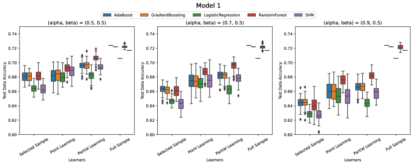
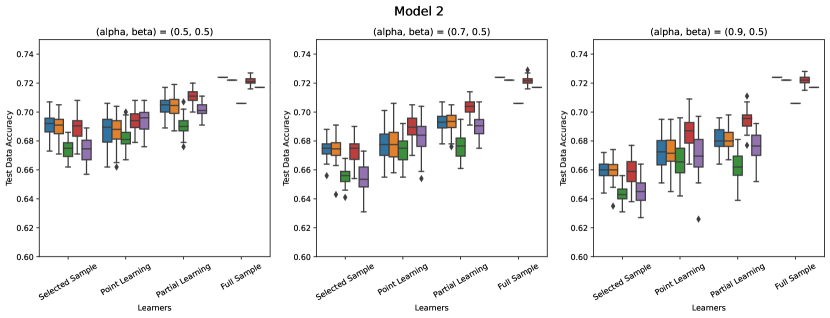
Figure 3: The accuracy scores of four learning methods with different confounding strength $\alpha=[0.5,0.7,0.9]$ and degree of missing $\beta=0.5$. The top graph reflects the results of Model 1 in decision generating process, while the bottom graph reveals the results of Model 2 in (D.1).

In this section, we conduct additional experiments under different degree of missingness $\beta=[1.0,0.5,0.25]$ as mentioned previously. Figures 3 and 4 report the testing accuracy of each method in $50$ replications with $\alpha\in\{0.5,0.7,0.9\}$ under the case of $\beta=0.5$ and $\beta=0.25$ respectively. As the parameter $\beta$ decreases, the size of the labeled dataset becomes smaller, and the performance of our methods and the ”selected sample” baseline all degrades. In spite of this, both ”point learning” and ”partial learning” methods dominates the ”selected sample” baseline on average. Interestingly, the ”partial learning” method has better performance than ”point learning” with higher average accuracy and lower variance.

Finally, we remark that the decision-maker assignment $Z$ plays different roles in different methods. Our proposed methods (”point learning” and ”partial learning”) treatment the decision-maker assignment $Z$ as an instrumental variable to correct for selection bias. In contrast, the baseline methods (”selected sample” and ”full sample”) do not necessarily need $Z$. However, for a fair comparison between our proposals and the baselines, we still incorporate $Z$ as a classification feature in the baseline methods, so they also use the information of $Z$.

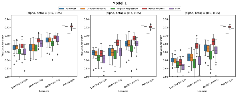
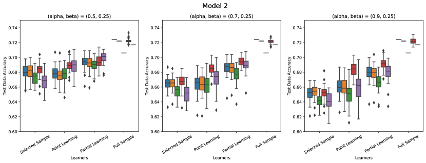
Figure 4: The accuracy scores of four learning methods with different confounding strength $\alpha=[0.5,0.7,0.9]$ and degree of missing $\beta=0.25$. The top graph reflects the results of Model 1 in decision generating process, while the bottom graph reveals the results of Model 2 in (D.1).

References

- Angrist and Imbens [1995] J. Angrist and G. Imbens. Identification and estimation of local average treatment effects, 1995.
- Angrist and Pischke [2009] J. D. Angrist and J.-S. Pischke. Mostly harmless econometrics: An empiricist’s companion. Princeton university press, 2009.
- Angrist et al. [1996] J. D. Angrist, G. W. Imbens, and D. B. Rubin. Identification of causal effects using instrumental variables. Journal of the American statistical Association, 91(434):444–455, 1996.
- Arnold et al. [2022] D. Arnold, W. Dobbie, and P. Hull. Measuring racial discrimination in bail decisions. American Economic Review, 112(9):2992–3038, 2022.
- Athey and Wager [2021] S. Athey and S. Wager. Policy learning with observational data. Econometrica, 89(1):133–161, 2021.
- Athey et al. [2019] S. Athey, J. Tibshirani, and S. Wager. Generalized random forests. The Annals of Statistics, 47(2):1148–1178, 2019.
- Bach [2021] F. Bach. Learning theory from first principles, 2021.
- Balke and Pearl [1994] A. Balke and J. Pearl. Counterfactual probabilities: Computational methods, bounds and applications. In Uncertainty Proceedings 1994, pages 46–54. Elsevier, 1994.
- Bartlett et al. [2006] P. L. Bartlett, M. I. Jordan, and J. D. McAuliffe. Convexity, classification, and risk bounds. Journal of the American Statistical Association, 101(473):138–156, 2006.
- Ben-Michael et al. [2021] E. Ben-Michael, D. J. Greiner, K. Imai, and Z. Jiang. Safe policy learning through extrapolation: Application to pre-trial risk assessment. arXiv preprint arXiv:2109.11679, 2021.
- Bertsimas and Fazel-Zarandi [2022] D. Bertsimas and M. M. Fazel-Zarandi. Prescriptive machine learning for public policy: The case of immigration enforcement. Under review, 2022.
- Chernozhukov et al. [2018] V. Chernozhukov, D. Chetverikov, M. Demirer, E. Duflo, C. Hansen, W. Newey, and J. Robins. Double/debiased machine learning for treatment and structural parameters, 2018.
- Cui and Tchetgen Tchetgen [2021] Y. Cui and E. Tchetgen Tchetgen. A semiparametric instrumental variable approach to optimal treatment regimes under endogeneity. Journal of the American Statistical Association, 116(533):162–173, 2021.
- De-Arteaga et al. [2018] M. De-Arteaga, A. Dubrawski, and A. Chouldechova. Learning under selective labels in the presence of expert consistency. arXiv preprint arXiv:1807.00905, 2018.
- De-Arteaga et al. [2021] M. De-Arteaga, V. Jeanselme, A. Dubrawski, and A. Chouldechova. Leveraging expert consistency to improve algorithmic decision support. arXiv preprint arXiv:2101.09648, 2021.
- D’Amour [2019] A. D’Amour. On multi-cause approaches to causal inference with unobserved counfounding: Two cautionary failure cases and a promising alternative. In The 22nd International Conference on Artificial Intelligence and Statistics, pages 3478–3486. PMLR, 2019.
- FICO [2018] FICO. Explainable machine learning challenge, 2018.
- Imbens and Rubin [2015] G. W. Imbens and D. B. Rubin. Causal inference in statistics, social, and biomedical sciences. Cambridge University Press, 2015.
- Kallus and Zhou [2021] N. Kallus and A. Zhou. Minimax-optimal policy learning under unobserved confounding. Management Science, 67(5):2870–2890, 2021.
- Kilbertus et al. [2020] N. Kilbertus, M. G. Rodriguez, B. Schölkopf, K. Muandet, and I. Valera. Fair decisions despite imperfect predictions. In International Conference on Artificial Intelligence and Statistics, pages 277–287. PMLR, 2020.
- Kleinberg et al. [2018] J. Kleinberg, H. Lakkaraju, J. Leskovec, J. Ludwig, and S. Mullainathan. Human decisions and machine predictions. The quarterly journal of economics, 133(1):237–293, 2018.
- Kling [2006] J. R. Kling. Incarceration length, employment, and earnings. American Economic Review, 96(3):863–876, 2006.
- Kosorok and Laber [2019] M. R. Kosorok and E. B. Laber. Precision medicine. Annual review of statistics and its application, 6:263–286, 2019.
- Laine et al. [2020] R. Laine, A. Hyttinen, and M. Mathioudakis. Evaluating decision makers over selectively labelled data: A causal modelling approach. In Discovery Science: 23rd International Conference, DS 2020, Thessaloniki, Greece, October 19–21, 2020, Proceedings 23, pages 3–18. Springer, 2020.
- Lakkaraju et al. [2017] H. Lakkaraju, J. Kleinberg, J. Leskovec, J. Ludwig, and S. Mullainathan. The selective labels problem: Evaluating algorithmic predictions in the presence of unobservables. In Proceedings of the 23rd ACM SIGKDD International Conference on Knowledge Discovery and Data Mining, pages 275–284, 2017.
- Little and Rubin [2019] R. J. Little and D. B. Rubin. Statistical analysis with missing data, volume 793. John Wiley & Sons, 2019.
- Manski and Pepper [1998] C. F. Manski and J. V. Pepper. Monotone instrumental variables with an application to the returns to schooling, 1998.
- Mueller-Smith [2015] M. Mueller-Smith. The criminal and labor market impacts of incarceration. Unpublished working paper, 18, 2015.
- Pu and Zhang [2021] H. Pu and B. Zhang. Estimating optimal treatment rules with an instrumental variable: A partial identification learning approach. Journal of the Royal Statistical Society: Series B (Statistical Methodology), 83(2):318–345, 2021.
- Qian and Murphy [2011] M. Qian and S. A. Murphy. Performance guarantees for individualized treatment rules. Annals of statistics, 39(2):1180, 2011.
- Rambachan et al. [2022] A. Rambachan, A. Coston, and E. Kennedy. Counterfactual risk assessments under unmeasured confounding. arXiv preprint arXiv:2212.09844, 2022.
- Rambachan et al. [2021] A. Rambachan et al. Identifying prediction mistakes in observational data. Harvard University, 2021.
- Shalev-Shwartz and Ben-David [2014] S. Shalev-Shwartz and S. Ben-David. Understanding machine learning: From theory to algorithms. Cambridge university press, 2014.
- Swanson et al. [2018] S. A. Swanson, M. A. Hernán, M. Miller, J. M. Robins, and T. S. Richardson. Partial identification of the average treatment effect using instrumental variables: review of methods for binary instruments, treatments, and outcomes. Journal of the American Statistical Association, 113(522):933–947, 2018.
- Vershynin [2018] R. Vershynin. High-dimensional probability: An introduction with applications in data science, volume 47. Cambridge university press, 2018.
- Wainwright [2019] M. J. Wainwright. High-dimensional statistics: A non-asymptotic viewpoint, volume 48. Cambridge University Press, 2019.
- Wang and Tchetgen [2018] L. Wang and E. T. Tchetgen. Bounded, efficient and multiply robust estimation of average treatment effects using instrumental variables. Journal of the Royal Statistical Society. Series B, Statistical methodology, 80(3):531, 2018.
- Wei [2021] D. Wei. Decision-making under selective labels: Optimal finite-domain policies and beyond. In International Conference on Machine Learning, pages 11035–11046. PMLR, 2021.
- Yang et al. [2022] Y. Yang, Y. Liu, and P. Naghizadeh. Adaptive data debiasing through bounded exploration. Advances in Neural Information Processing Systems, 35:1516–1528, 2022.
- Zhao et al. [2012] Y. Zhao, D. Zeng, A. J. Rush, and M. R. Kosorok. Estimating individualized treatment rules using outcome weighted learning. Journal of the American Statistical Association, 107(499):1106–1118, 2012.