Fixed-Budget Best-Arm Identification with Heterogeneous Reward Variances

Abstract

We study the problem of best-arm identification (BAI) in the fixed-budget setting with heterogeneous reward variances. We propose two variance-adaptive BAI algorithms for this setting: $\tt SHVar$ for known reward variances and $\tt SHAdaVar$ for unknown reward variances. The key idea in our algorithms is to adaptively allocate more budget to arms with higher reward variances. The main algorithmic novelty is in the design of $\tt SHAdaVar$, which allocates budget greedily based on overestimating unknown reward variances. We bound the probabilities of misidentifying best arms in both $\tt SHVar$ and $\tt SHAdaVar$. Our analyses rely on novel lower bounds on the number of arm pulls in BAI that do not require closed-form solutions to the budget allocation problem. One of our budget allocation problems is equivalent to the optimal experiment design with unknown variances and thus of a broad interest. We also evaluate our algorithms on synthetic and real-world problems. In most settings, $\tt SHVar$ and $\tt SHAdaVar$ outperform all prior algorithms.

1 Introduction

The problem of best-arm identification (BAI) in the fixed-budget setting is a pure exploration bandit problem which can be briefly described as follows. An agent interacts with a stochastic multi-armed bandit with $K$ arms and its goal is to identify the arm with the highest mean reward within a fixed budget $n$ of arm pulls [Bubeck et al., 2009, Audibert et al., 2010]. This problem arises naturally in many applications in practice, such as online advertising, recommender systems, and vaccine tests [Lattimore and Szepesvari, 2019]. It is also common in applications where observations are costly, such as Bayesian optimization [Krause et al., 2008]. Another commonly studied setting is fixed-confidence BAI [Even-Dar et al., 2006, Soare et al., 2014]. Here the goal is to identify the best arm within a prescribed confidence level while minimizing the budget. Some works also studied both settings [Gabillon et al., 2012, Karnin et al., 2013, Kaufmann et al., 2016].

Our work can be motivated by the following example. Consider an A/B test where the goal is to identify a movie with the highest average user rating from a set of $K$ movies. This problem can be formulated as BAI by treating the movies as arms and user ratings as stochastic rewards. Some movies get either unanimously good or bad ratings, and thus their ratings have a low variance. Others get a wide range of ratings, because they are rated highly by their target audience and poorly by others; and hence their ratings have a high variance. For this setting, we can design better BAI policies that take the variance into account. Specifically, movies with low-variance ratings can be exposed to fewer users in the A/B test than movies with high-variance ratings.

An analogous synthetic example is presented in Figure 1. In this example, reward variances increase with mean arm rewards for a half of the arms, while the remaining arms have very low variances. The knowledge of the reward variances can be obviously used to reduce the number of pulls of arms with low-variance rewards. However, in practice, the reward variances are rarely known in advance, such as in our motivating A/B testing example, and this makes the design and analysis of variance-adaptive BAI algorithms challenging. We revisit these two examples in our empirical studies in Section 5.

We propose and analyze two variance-adaptive BAI algorithms: $\tt SHVar$ and $\tt SHAdaVar$. $\tt SHVar$ assumes that the reward variances are known and is a stepping stone for our fully-adaptive BAI algorithm $\tt SHAdaVar$, which estimates them. $\tt SHAdaVar$ utilizes high-probability upper confidence bounds on the reward variances. Both algorithms are motivated by sequential halving ($\tt SH$) of Karnin et al. [2013], a near-optimal solution for fixed-budget BAI with homogeneous reward variances.

Our main contributions are:

• We design two variance-adaptive algorithms for fixed-budget BAI: $\tt SHVar$ for known reward variances and $\tt SHAdaVar$ for unknown reward variances. $\tt SHAdaVar$ is only a third algorithm for this setting [Gabillon et al., 2011, Faella et al., 2020] and only a second that can be implemented as analyzed [Faella et al., 2020]. The key idea in $\tt SHAdaVar$ is to solve a budget allocation problem with unknown reward variances by a greedy algorithm that overestimates them. This idea can be applied to other elimination algorithms in the cumulative regret setting [Auer and Ortner, 2010] and is of independent interest to the field of optimal experiment design [Pukelsheim, 1993].

• We prove upper bounds on the probability of misidentifying the best arm for both $\tt SHVar$ and $\tt SHAdaVar$. The analysis of $\tt SHVar$ extends that of Karnin et al. [2013] to heterogeneous variances. The analysis of $\tt SHAdaVar$ relies on a novel lower bound on the number of pulls of an arm that scales linearly with its unknown reward variance. This permits an analysis of sequential halving without requiring a closed form for the number of pulls of each arm.

• We evaluate our methods empirically on Gaussian bandits and the MovieLens dataset [Lam and Herlocker, 2016]. In most settings, $\tt SHVar$ and $\tt SHAdaVar$ outperform all prior algorithms.

The paper is organized as follows. In Section 2, we present the fixed-budget BAI problem. We present our algorithms in Section 3 and analyze them in Section 4. The algorithms are empirically evaluated in Section 5. We review prior works in Section 6 and conclude in Section 7.

2 Setting

We use the following notation. Random variables are capitalized, except for Greek letters like $\mu$. For any positive integer $n$, we define $[n]=\left\{1,\dots,n\right\}$. The indicator function is denoted by $\mathds{1}\!\left\{\cdot\right\}$. The $i$-th entry of vector $v$ is $v_{i}$. If the vector is already indexed, such as $v_{j}$, we write $v_{j,i}$. The big O notation up to logarithmic factors is $\tilde{O}$.

We have a stochastic bandit with $K$ arms and denote the set of arms by $\mathcal{A}=[K]$. When the arm is pulled, its reward is drawn i.i.d. from its reward distribution. The reward distribution of arm $i\in\mathcal{A}$ is sub-Gaussian with mean $\mu_{i}$ and variance proxy $\sigma^{2}_{i}$. The best arm is the arm with the highest mean reward,

$$\textstyle i_{*}=\operatorname*{arg\,max\,}_{i\in\mathcal{A}}\mu_{i}\,.$$

Without loss of generality, we make an assumption that the arms are ordered as $\mu_{1}>\mu_{2}\geq\ldots\geq\mu_{K}$. Therefore, arm $i_{*}=1$ is a unique best arm. The agent has a budget of $n$ observations and the goal is to identify $i_{*}$ as accurately as possible after pulling all arms $n$ times. Specifically, let $\hat{I}$ denote the arm returned by the agent after $n$ pulls. Then our objective is to minimize the probability of misidentifying the best arm $\mathbb{P}\left(\hat{I}\neq i_{*}\right)$, which we also call a mistake probability. This setting is known as fixed-budget BAI [Bubeck et al., 2009, Audibert et al., 2010]. When observations are costly, it is natural to limit them by a fixed budget $n$.

Another commonly studied setting is fixed-confidence BAI [Even-Dar et al., 2006, Soare et al., 2014]. Here the agent is given an upper bound on the mistake probability $\delta$ as an input and the goal is to attain $\mathbb{P}\left(\hat{I}\neq i_{*}\right)\leq\delta$ at minimum budget $n$. Some works also studied both the fixed-budget and fixed-confidence settings [Gabillon et al., 2012, Karnin et al., 2013, Kaufmann et al., 2016].

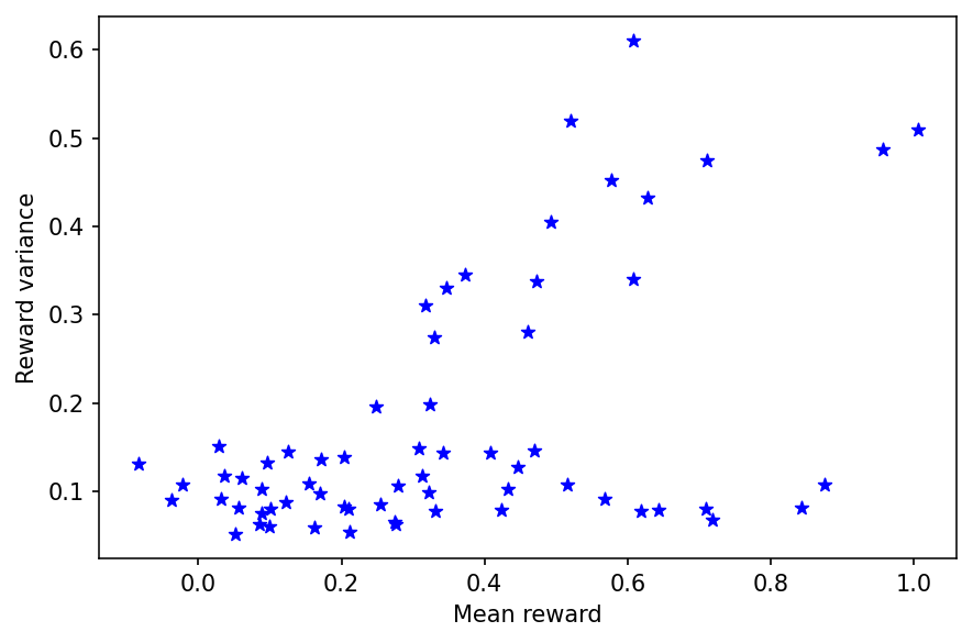
Figure 1: Mean rewards and variances for $K=64$ arms in the Gaussian bandit in Section 5.1.

3 Algorithms

A near-optimal solution for fixed-budget BAI with homogeneous reward variances is sequential halving [Karnin et al., 2013]. The key idea is to sequentially eliminate suboptimal arms in $\log_{2}K$ stages. In each stage, all arms are pulled equally and the worst half of the arms are eliminated at the end of the stage. At the end of the last stage, only one arm $\hat{I}$ remains and that arm is the estimated best arm.

Algorithm 1 Meta-algorithm for sequential halving.

1:Input: Budget $n$, base algorithm $\tt Alg$

2:

3:Number of stages $m\leftarrow\left\lceil\log_{2}K\right\rceil$

4:$\mathcal{A}_{1}\leftarrow\mathcal{A}$

5:for $s=1,\dots,m$ do

6:     Per-stage budget $\displaystyle n_{s}\leftarrow\left\lfloor n/m\right\rfloor$

7:     for $t=1,\dots,n_{s}$ do

8:         $I_{s,t}\leftarrow\tt Alg(s,t)$

9:         Observe reward $Y_{s,t,I_{s,t}}$ of arm $I_{s,t}$      

10:     for $i\in\mathcal{A}_{s}$ do

11:         $\displaystyle N_{s,i}\leftarrow\sum_{t=1}^{n_{s}}\mathds{1}\!\left\{I_{s,t}=i\right\}$

12:         $\displaystyle\hat{\mu}_{s,i}\leftarrow\frac{1}{N_{s,i}}\sum_{t=1}^{n_{s}}\mathds{1}\!\left\{I_{s,t}=i\right\}Y_{s,t,i}$      

13:     $\mathcal{A}_{s+1}\leftarrow\left\{\textrm{$\left\lceil\left|\mathcal{A}_{s}\right|/2\right\rceil$ arms $i\in\mathcal{A}_{s}$ with highest $\hat{\mu}_{s,i}$}\right\}$

14:

15:Output: The last remaining arm $\hat{I}$ in $\mathcal{A}_{m+1}$

Algorithm 2 $\tt SH$: Pulled arm in sequential halving.

1:Input: Stage $s$, round $t$

2:

3:$k\leftarrow(t-1)\bmod\left|\mathcal{A}_{s}\right|+1$

4:$I_{s,t}\leftarrow\textrm{$k$-th arm in $\mathcal{A}_{s}$}$

5:

6:Output: Arm to pull $I_{s,t}$

Algorithm 3 $\tt SHVar$: Pulled arm in sequential halving with known heterogeneous reward variances.

1:Input: Stage $s$, round $t$

2:

3:for $i\in\mathcal{A}_{s}$ do

4:     $\displaystyle N_{s,t,i}\leftarrow\sum_{\ell=1}^{t-1}\mathds{1}\!\left\{I_{s,\ell}=i\right\}$

5:$\displaystyle I_{s,t}\leftarrow\operatorname*{arg\,max\,}_{i\in\mathcal{A}_{s}}\frac{\sigma_{i}^{2}}{N_{s,t,i}}$

6:

7:Output: Arm to pull $I_{s,t}$

The main algorithmic contribution of our work is that we generalize sequential halving of Karnin et al. [2013] to heterogeneous reward variances. All of our algorithms can be viewed as instances of a meta-algorithm (Algorithm 1), which we describe in detail next. Its inputs are a budget $n$ on the number of observations and base algorithm $\tt Alg$. The meta-algorithm has $m$ stages (line 2) and the budget is divided equally across the stages, with a per-stage budget $n_{s}=\left\lfloor n/m\right\rfloor$ (line 5). In stage $s$, all remaining arms $\mathcal{A}_{s}$ are pulled according to $\tt Alg$ (lines 6–8). At the end of stage $s$, the worst half of the remaining arms, as measured by their estimated mean rewards, is eliminated (lines 9–12). Here $Y_{s,t,i}$ is the stochastic reward of arm $i$ in round $t$ of stage $s$, $I_{s,t}\in\mathcal{A}_{s}$ is the pulled arm in round $t$ of stage $s$, $N_{s,i}$ is the number of pulls of arm $i$ in stage $s$, and $\hat{\mu}_{s,i}$ is its mean reward estimate from all observations in stage $s$.

The sequential halving of Karnin et al. [2013] is an instance of Algorithm 1 for $\tt Alg=\tt SH$. The pseudocode of $\tt SH$, which pulls all arms in stage $s$ equally, is in Algorithm 2. We call the resulting algorithm $\tt SH$. This algorithm misidentifies the best arm with probability [Karnin et al., 2013]

$$\mathbb{P}\left(\hat{I}\neq 1\right)\leq 3\log_{2}K\exp\left[-\frac{n}{8H_{2}\log_{2}K}\right]\,,$$ (1)

where

$$H_{2}=\max_{i\in\mathcal{A}\setminus\left\{1\right\}}\frac{i}{\Delta_{i}^{2}}$$ (2)

is a complexity parameter and $\Delta_{i}=\mu_{1}-\mu_{i}$ is the suboptimality gap of arm $i$. The bound in (1) decreases as budget $n$ increases and problem complexity $H_{2}$ decreases.

$\tt SH$ is near optimal only in the setting of homogeneous reward variances. In this work, we study the general setting where the reward variances of arms vary, potentially as extremely as in our motivating example in Figure 1. In this example, $\tt SH$ would face arms with both low and high variances in each stage. A variance-adaptive $\tt SH$ could adapt its budget allocation in each stage to the reward variances and thus eliminate suboptimal arms more effectively.

3.1 Known Heterogeneous Reward Variances

We start with the setting of known reward variances. Let

$$\sigma_{i}^{2}=\mathrm{var}\left[Y_{s,t,i}\right]=\mathbb{E}\left[(Y_{s,t,i}-\mu_{i})^{2}\right]$$ (3)

be a known reward variance of arm $i$. Our proposed algorithm is an instance of Algorithm 1 for $\tt Alg=\tt SHVar$. The pseudocode of $\tt SHVar$ is in Algorithm 3. The key idea is to pull the arm with the highest variance of its mean reward estimate. The variance of the mean reward estimate of arm $i$ in round $t$ of stage $s$ is $\sigma_{i}^{2}/N_{s,t,i}$, where $\sigma_{i}^{2}$ is the reward variance of arm $i$ and $N_{s,t,i}$ is the number of pulls of arm $i$ up to round $t$ of stage $s$. We call the resulting algorithm $\tt SHVar$.

Note that $\tt SH$ is an instance of $\tt SHVar$. Specifically, when all $\sigma_{i}=\sigma$ for some $\sigma>0$, $\tt SHVar$ pulls all arms equally, as in $\tt SH$. $\tt SHVar$ can be also viewed as pulling any arm $i$ in stage $s$ for

$$N_{s,i}\approx\frac{\sigma_{i}^{2}}{\sum_{j\in\mathcal{A}_{s}}\sigma_{j}^{2}}n_{s}$$ (4)

times. This is stated formally and proved below.

Lemma 1.

Fix stage $s$ and let the ideal number of pulls of arm $i\in\mathcal{A}_{s}$ be

$$\lambda_{s,i}=\frac{\sigma_{i}^{2}}{\sum_{j\in\mathcal{A}_{s}}\sigma_{j}^{2}}n_{s}\,.$$

Let all $\lambda_{s,i}$ be integers. Then $\tt SHVar$ pulls arm $i$ in stage $s$ exactly $\lambda_{s,i}$ times.

Proof.

First, suppose that $\tt SHVar$ pulls each arm $i$ exactly $\lambda_{s,i}$ times. Then the variances of all mean reward estimates at the end of stage $s$ are identical, because

$$\frac{\sigma_{i}^{2}}{N_{s,i}}=\frac{\sigma_{i}^{2}}{\lambda_{s,i}}=\frac{\sigma_{i}^{2}}{\frac{\sigma_{i}^{2}}{\sum_{j\in\mathcal{A}_{s}}\sigma_{j}^{2}}n_{s}}=\frac{\sum_{j\in\mathcal{A}_{s}}\sigma_{j}^{2}}{n_{s}}\,.$$

Now suppose that this is not true. This implies that there exists an over-pulled arm $i\in\mathcal{A}_{s}$ and an under-pulled arm $k\in\mathcal{A}_{s}$ such that

$$\frac{\sigma_{i}^{2}}{N_{s,i}}<\frac{\sum_{j\in\mathcal{A}_{s}}\sigma_{j}^{2}}{n_{s}}<\frac{\sigma_{k}^{2}}{N_{s,k}}\,.$$ (5)

Since arm $i\in\mathcal{A}_{s}$ is over-pulled and $\lambda_{s,i}$ is an integer, there must exist a round $t\in[n_{s}]$ such that

$$\frac{\sigma_{i}^{2}}{N_{s,t,i}}=\frac{\sigma_{i}^{2}}{\lambda_{s,i}}=\frac{\sum_{j\in\mathcal{A}_{s}}\sigma_{j}^{2}}{n_{s}}\,.$$

Let $t$ be the last round where this equality holds, meaning that arm $i$ is pulled in round $t$.

Now we combine the second inequality in (5) with $N_{s,k}\geq N_{s,t,k}$, which holds by definition, and get

$$\frac{\sum_{j\in\mathcal{A}_{s}}\sigma_{j}^{2}}{n_{s}}<\frac{\sigma_{k}^{2}}{N_{s,k}}\leq\frac{\sigma_{k}^{2}}{N_{s,t,k}}\,.$$

The last two sets of inequalities lead to a contradiction. On one hand, we know that arm $i$ is pulled in round $t$. On the other hand, we have $\sigma_{i}^{2}/N_{s,t,i}<\sigma_{k}^{2}/N_{s,t,k}$, which means that arm $i$ cannot be pulled. This completes the proof. ∎

Lemma 1 says that each arm $i\in\mathcal{A}_{s}$ is pulled $O(\sigma_{i}^{2})$ times. Since the mean reward estimate of arm $i$ at the end of stage $s$ has variance $\sigma_{i}^{2}/N_{s,i}$, the variances of all estimates at the end of stage $s$ are identical, $\left(\sum_{i\in\mathcal{A}_{s}}\sigma_{i}^{2}\right)/n_{s}$. This relates our problem to the G-optimal design [Pukelsheim, 1993]. Specifically, the $G$-optimal design for independent experiments $i\in\mathcal{A}_{s}$ is an allocation of observations $(N_{s,i})_{i\in\mathcal{A}_{s}}$ such that $\sum_{i\in\mathcal{A}_{s}}N_{s,i}=n_{s}$ and the maximum variance

$$\max_{i\in\mathcal{A}_{s}}\frac{\sigma_{i}^{2}}{N_{s,i}}$$ (6)

is minimized. This happens precisely when all $\sigma_{i}^{2}/N_{s,i}$ are identical, when $N_{s,i}=\lambda_{s,i}$ for $\lambda_{s,i}$ in Lemma 1.

3.2 Unknown Heterogeneous Reward Variances

Our second proposal is an algorithm for unknown reward variances. One natural idea, which is expected to be practical but hard to analyze, is to replace $\sigma_{i}^{2}$ in $\tt SHVar$ with its empirical estimate from the past $t-1$ rounds in stage $s$,

$$\hat{\sigma}_{s,t,i}^{2}=\frac{1}{N_{s,t,i}-1}\sum_{\ell=1}^{t-1}\mathds{1}\!\left\{I_{s,\ell}=i\right\}(Y_{s,\ell,i}-\hat{\mu}_{s,t,i})^{2}\,,$$

where

$$\hat{\mu}_{s,t,i}=\frac{1}{N_{s,t,i}}\sum_{\ell=1}^{t-1}\mathds{1}\!\left\{I_{s,\ell}=i\right\}Y_{s,\ell,i}$$

is the empirical mean reward of arm $i$ in round $t$ of stage $s$. This design would be hard to analyze because $\hat{\sigma}_{s,t,i}$ can underestimate $\sigma_{i}$, and thus is not an optimistic estimate.

The key idea in our solution is to act optimistically using an upper confidence bound (UCB) on the reward variance. To derive it, we make an assumption that the reward noise is Gaussian. Specifically, the reward of arm $i$ in round $t$ of stage $s$ is distributed as $Y_{s,t,i}\sim\mathcal{N}(\mu_{i},\sigma_{i}^{2})$. This allows us to derive the following upper and lower bounds on the unkown variance $\sigma_{i}^{2}$.

Algorithm 4 $\tt SHAdaVar$: Pulled arm in sequential halving with unknown heterogeneous reward variances.

1:Input: Stage $s$, round $t$

2:

3:if $t\leq\left|\mathcal{A}_{s}\right|(4\log(1/\delta)+1)$ then

4:     $k\leftarrow(t-1)\bmod\left|\mathcal{A}_{s}\right|+1$

5:     $I_{s,t}\leftarrow\textrm{$k$-th arm in $\mathcal{A}_{s}$}$

6:else

7:     for $i\in\mathcal{A}_{s}$ do

8:         $\displaystyle N_{s,t,i}\leftarrow\sum_{\ell=1}^{t-1}\mathds{1}\!\left\{I_{s,\ell}=i\right\}$      

9:     $\displaystyle I_{s,t}\leftarrow\operatorname*{arg\,max\,}_{i\in\mathcal{A}_{s}}\frac{U_{s,t,i}}{N_{s,t,i}}$

10:

11:Output: Arm to pull $I_{s,t}$

Lemma 2.

Fix stage $s$, round $t\in[n_{s}]$, arm $i\in\mathcal{A}_{s}$, and failure probability $\delta\in(0,1)$. Let

$$N=N_{s,t,i}-1$$

and suppose that $N>4\log(1/\delta)$. Then

$$\mathbb{P}\left(\sigma_{i}^{2}\geq\frac{\hat{\sigma}_{s,t,i}^{2}}{1-2\sqrt{\frac{\log(1/\delta)}{N}}}\right)\leq\delta$$

holds with probability at least $1-\delta$. Analogously,

$$\mathbb{P}\left(\hat{\sigma}_{s,t,i}^{2}\geq\sigma_{i}^{2}\left[1+2\sqrt{\frac{\log(1/\delta)}{N}}+\frac{2\log(1/\delta)}{N}\right]\right)\leq\delta$$

holds with probability at least $1-\delta$.

Proof.

The first claim is proved as follows. By Cochran’s theorem, we have that $\hat{\sigma}_{s,t,i}^{2}N/\sigma_{i}^{2}$ is a $\chi^{2}$ random variable with $N$ degrees of freedom. Its concentration was analyzed in Laurent and Massart [2000]. More specifically, by (4.4) in Laurent and Massart [2000], an immediate corollary of their Lemma 1, we have

$$\mathbb{P}\left(N-\frac{\hat{\sigma}_{s,t,i}^{2}N}{\sigma_{i}^{2}}\geq 2\sqrt{N\log(1/\delta)}\right)\leq\delta\,.$$

Now we divide both sides in the probability by $N$, multiply by $\sigma_{i}^{2}$, and rearrange the formula as

$$\mathbb{P}\left(\sigma_{i}^{2}\left(1-2\sqrt{\log(1/\delta)/N}\right)\geq\hat{\sigma}_{s,t,i}^{2}\right)\leq\delta\,.$$

When $1-2\sqrt{\log(1/\delta)/N}>0$, we can divide both sides by it and get the first claim in Lemma 2.

The second claim is proved analogously. Specifically, by (4.3) in Laurent and Massart [2000], an immediate corollary of their Lemma 1, we have

$$\mathbb{P}\left(\frac{\hat{\sigma}_{s,t,i}^{2}N}{\sigma_{i}^{2}}-N\geq 2\sqrt{N\log(1/\delta)}+2\log(1/\delta)\right)\leq\delta\,.$$

Now we divide both sides in the probability by $N$, multiply by $\sigma_{i}^{2}$, and obtain the second claim in Lemma 2. This concludes the proof. ∎

By Lemma 2, when $N_{s,t,i}>4\log(1/\delta)+1$,

$$U_{s,t,i}=\frac{\hat{\sigma}_{s,t,i}^{2}}{1-2\sqrt{\frac{\log(1/\delta)}{N_{s,t,i}-1}}}$$ (7)

is a high-probability upper bound on the reward variance of arm $i$ in round $t$ of stage $s$, which holds with probability at least $1-\delta$. This bound decreases as the number of observations $N_{s,t,i}$ increases and confidence $\delta$ decreases. To apply the bound across multiple stages, rounds, and arms, we use a union bound.

The bound in (7) leads to our algorithm that overestimates the variance. The algorithm is an instance of Algorithm 1 for $\tt Alg=\tt SHAdaVar$. The pseudocode of $\tt SHAdaVar$ is in Algorithm 4. To guarantee $N_{s,t,i}>4\log(1/\delta)+1$, we pull all arms $\mathcal{A}_{s}$ in any stage $s$ for $4\log(1/\delta)+1$ times initially. We call the resulting algorithm $\tt SHAdaVar$.

Note that $\tt SHAdaVar$ can be viewed as a variant of $\tt SHVar$ where $U_{s,t,i}$ replaces $\sigma_{i}^{2}$. Therefore, it can also be viewed as solving the G-optimal design in (6) without knowing reward variances $\sigma_{i}^{2}$; and $\tt SHAdaVar$ is of a broader interest to the optimal experiment design community [Pukelsheim, 1993]. We also note that the assumption of Gaussian noise in the design of $\tt SHAdaVar$ is limiting. To address this issue, we experiment with non-Gaussian noise in Section 5.2.

4 Analysis

This section comprises three analyses. In Section 4.1, we bound the probability that $\tt SHVar$, an algorithm that knows reward variances, misidentifies the best arm. In Section 4.2, we provide an alternative analysis that does not rely on the closed form in (4). Finally, in Section 4.3, we bound the probability that $\tt SHAdaVar$, an algorithm that learns reward variances, misidentifies the best arm.

All analyses are under the assumption of Gaussian reward noise. Specifically, the reward of arm $i$ in round $t$ of stage $s$ is distributed as $Y_{s,t,i}\sim\mathcal{N}(\mu_{i},\sigma_{i}^{2})$.

4.1 Error Bound of $\tt SHVar$

We start with analyzing $\tt SHVar$, which is a stepping stone for analyzing $\tt SHAdaVar$. To simplify the proof, we assume that both $m$ and $n_{s}$ are integers. We also assume that all budget allocations have integral solutions in Lemma 1.

Theorem 3.

$\tt SHVar$ misidentifies the best arm with probability

$$\mathbb{P}\left(\hat{I}\neq 1\right)\leq 2\log_{2}K\exp\left[-\frac{n\Delta_{\min}^{2}}{4\log_{2}K\sum_{j\in\mathcal{A}}\sigma_{j}^{2}}\right]\,,$$

where $\Delta_{\min}=\mu_{1}-\mu_{2}$ is the minimum gap.

Proof.

The claim is proved in Appendix A. We follow the outline in Karnin et al. [2013]. The novelty is in extending the proof to heterogeneous reward variances. This requires a non-uniform budget allocation, where arms with higher reward variances are pulled more (Lemma 1). ∎

The bound in Theorem 3 depends on all quantities as expected. It decreases as budget $n$ and minimum gap $\Delta_{\min}$ increase, and the number of arms $K$ and variances $\sigma_{j}^{2}$ decrease. $\tt SHVar$ reduces to $\tt SH$ in Karnin et al. [2013] when $\sigma_{i}^{2}=1/4$ for all arms $i\in\mathcal{A}$. The bounds of $\tt SH$ and $\tt SHVar$ become comparable when we apply $H_{2}\leq K/\Delta_{\min}^{2}$ in (1) and note that $\sum_{j\in\mathcal{A}}\sigma_{j}^{2}=K/4$ in Theorem 3. The extra factor of $8$ in the exponent of (1) is due to a different proof, which yields a finer dependence on gaps.

4.2 Alternative Error Bound of $\tt SHVar$

Now we analyze $\tt SHVar$ differently. The resulting bound is weaker than that in Theorem 3 but its proof can be easily extended to $\tt SHAdaVar$.

Theorem 4.

$\tt SHVar$ misidentifies the best arm with probability

$$\mathbb{P}\left(\hat{I}\neq 1\right)\leq 2\log_{2}K\exp\left[-\frac{(n-K\log K)\Delta_{\min}^{2}}{4\sigma_{\max}^{2}K\log_{2}K}\right]\,,$$

where $\Delta_{\min}=\mu_{1}-\mu_{2}$ is the minimum gap and $\sigma_{\max}^{2}=\max_{i\in\mathcal{A}}\sigma_{i}^{2}$ is the maximum reward variance.

Proof.

The claim is proved in Appendix B. The key idea in the proof is to derive a lower bound on the number of pulls of any arm $i$ in stage $s$, instead of using the closed form of $N_{s,i}$ in (4). The lower bound is

$$N_{s,i}\geq\frac{\sigma_{i}^{2}}{\sigma_{\max}^{2}}\left(\frac{n_{s}}{\left|\mathcal{A}_{s}\right|}-1\right)\,.$$

An important property of the bound is that it is $\Omega(\sigma_{i}^{2}n_{s})$, similarly to $N_{s,i}$ in (4). Therefore, the rest of the proof is similar to that of Theorem 3. ∎

As in Theorem 3, the bound in Theorem 4 depends on all quantities as expected. It decreases as budget $n$ and minimum gap $\Delta_{\min}$ increase, and the number of arms $K$ and maximum variance $\sigma_{\max}^{2}$ decrease. The bound approaches that in Theorem 3 when all reward variances are identical.

4.3 Error Bound of $\tt SHAdaVar$

Now we analyze $\tt SHAdaVar$.

Theorem 5.

Suppose that $\delta<1/(Kn)$ and

$$n\geq K\log_{2}K(4\log(Kn/\delta)+1)\,.$$

Then $\tt SHAdaVar$ misidentifies the best arm with probability

$$\mathbb{P}\left(\hat{I}\neq 1\right)\leq 2\log_{2}K\exp\left[-\alpha\frac{(n-K\log K)\Delta_{\min}^{2}}{4\sigma_{\max}^{2}K\log_{2}K}\right]\,,$$

where $\Delta_{\min}$ and $\sigma_{\max}^{2}$ are defined in Theorem 4, and

$$\alpha=\frac{1-2\sqrt{\frac{\log(Kn/\delta)}{n/K-2}}}{1+2\sqrt{\frac{\log(Kn/\delta)}{n/K-2}}+\frac{2\log(Kn/\delta)}{n/K-2}}\,.$$

Proof.

The claim is proved in Appendix C. The key idea in the proof is to derive a lower bound on the number of pulls of any arm $i$ in stage $s$, similarly to that in Theorem 4. The lower bound is

$$N_{s,i}\geq\frac{\sigma_{i}^{2}}{\sigma_{\max}^{2}}\alpha(\left|\mathcal{A}_{s}\right|,n_{s},\delta)\left(\frac{n_{s}}{\left|\mathcal{A}_{s}\right|}-1\right)$$

and holds with probability at least $1-\delta$. Since the bound is $\Omega(\sigma_{i}^{2}n_{s})$, as in the proof of Theorem 4, the rest of the proof is similar. The main difference from Theorem 4 is in factor $\alpha(\left|\mathcal{A}_{s}\right|,n_{s},\delta)$, which converges to $1$ as $n_{s}\to\infty$. ∎

The bound in Theorem 5 depends on all quantities as expected. It decreases as budget $n$ and minimum gap $\Delta_{\min}$ increase, and the number of arms $K$ and maximum variance $\sigma_{\max}^{2}$ decrease. As $n\to\infty$, we get $\alpha\to 1$ and the bound converges to that in Theorem 4.

5 Experiments

In this section, we empirically evaluate our proposed algorithms, $\tt SHVar$ and $\tt SHAdaVar$, and compare them to algorithms from prior works. We choose the following baselines: uniform allocation ($\tt Unif$), sequential halving ($\tt SH$) [Karnin et al., 2013], gap-based exploration ($\tt GapE$) [Gabillon et al., 2011], gap-based exploration with variance ($\tt GapE\mathchar 45\relax V$) [Gabillon et al., 2011], and variance-based rejects ($\tt VBR$) [Faella et al., 2020].

$\tt Unif$ allocates equal budget to all arms and $\tt SH$ was originally proposed for homogeneous reward variances. Neither $\tt Unif$ nor $\tt SH$ can adapt to heterogenuous reward variances. $\tt GapE$, $\tt GapE\mathchar 45\relax V$ and $\tt VBR$ are variance-adaptive BAI methods from related works (Section 6). In $\tt GapE$, we use $H$ from Theorem 1 of Gabillon et al. [2011]. In $\tt GapE\mathchar 45\relax V$, we use $H$ from Theorem 2 of Gabillon et al. [2011]. Both $\tt GapE$ and $\tt GapE\mathchar 45\relax V$ assume bounded reward distributions with support $[0,b]$. We choose $b=\max_{i\in\mathcal{A}}\mu_{i}+\sigma_{i}\sqrt{\log n}$, since this is a high-probability upper bound on the absolute value of $n$ independent observations from $\mathcal{N}(\mu_{i},\sigma_{i}^{2})$. In $\tt SHAdaVar$, we set $\delta=0.05$, and thus our upper bounds on reward variances hold with probability $0.95$. In $\tt VBR$, $\gamma=1.96$, which means that the mean arm rewards lie between their upper and lower bounds with probability $0.95$. Faella et al. [2020] showed that $\tt VBR$ performs well with Gaussian noise when $\gamma\approx 2$. All reported results are averaged over $5\,000$ runs.

$\tt GapE$ and $\tt GapE\mathchar 45\relax V$ have $O(\exp[-cn/H])$ error bounds on the probability of misidentifying the best arm, where $n$ is the budget, $H$ is the complexity parameter, and $c=1/144$ for $\tt GapE$ and $c=1/512$ for $\tt GapE\mathchar 45\relax V$. Our error bounds are $O(\exp[-c^{\prime}n/H^{\prime}])$, where $H^{\prime}$ is a comparable complexity parameter and $c^{\prime}=1/(4\log_{2}K)$. Even for moderate $K$, $c\ll c^{\prime}$. Therefore, when $\tt SHVar$ and $\tt SHAdaVar$ are implemented as analyzed, they provide stronger guarantees on identifying the best arm than $\tt GapE$ and $\tt GapE\mathchar 45\relax V$. To make the algorithms comparable, we set $H$ of $\tt GapE$ and $\tt GapE\mathchar 45\relax V$ to $Hc/c^{\prime}$, by increasing their confidence widths. Since $H$ is an input to both $\tt GapE$ and $\tt GapE\mathchar 45\relax V$, note that they have an advantage over our algorithms that do not require it.

5.1 Synthetic Experiments

Our first experiment is on a Gaussian bandit with $K$ arms. The mean reward of arm $i$ is $\mu_{i}=1-\sqrt{(i-1)/K}$. We choose this setting because $\tt SH$ is known to perform well in it. Specifically, note that the complexity parameter $H_{2}$ in (2) is minimized when $i/\Delta_{i}^{2}$ are equal for all $i\in\mathcal{A}\setminus\left\{1\right\}$. For our $\mu_{i}$, $\Delta_{i}^{2}=(i-1)/K\approx i/K$ and thus $i/\Delta_{i}^{2}\approx K$. We set the reward variance as $\sigma^{2}_{i}=0.9\mu^{2}_{i}+0.1$ when arm $i$ is even and $\sigma^{2}_{i}=0.1$ when arm $i$ is odd. We additionally perturb $\mu_{i}$ and $\sigma_{i}^{2}$ with additive $\mathcal{N}(0,0.05^{2})$ and multiplicative $\mathrm{Unif}(0.5,1.5)$ noise, respectively. We visualize the mean rewards $\mu_{i}$ and the corresponding variances $\sigma^{2}_{i}$, for $K=64$ arms, in Figure 1. The variances are chosen so that every stage of sequential halving involves both high-variance and low-variance arms. Therefore, an algorithm that adapts its budget allocation to the reward variances of the remaining arms eliminates the best arm with a lower probability than the algorithm that does not.

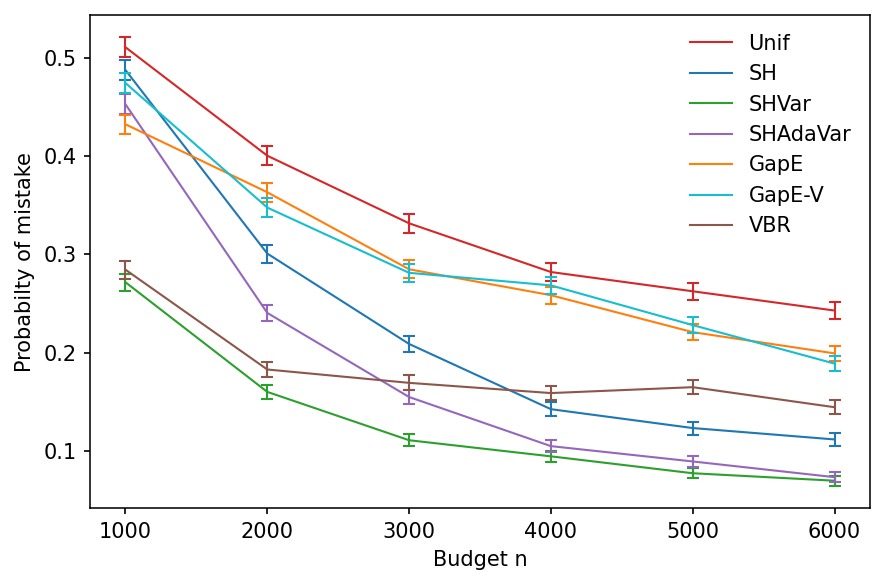
Figure 2: Probability of misidentifying the best arm in the Gaussian bandit in Section 5.1, as budget $n$ increases. The number of arms is $K=64$ and the results are averaged over $5\,000$ runs.

In Figure 2, we report the probability of misidentifying the best arm among $K=64$ arms (Figure 1) as budget $n$ increases. As expected, the naive algorithm $\tt Unif$ performs the worst. $\tt GapE$ and $\tt GapE\mathchar 45\relax V$ perform only slightly better. When the algorithms have comparable error guarantees to $\tt SHVar$ and $\tt SHAdaVar$, their confidence intervals are too wide to be practical. $\tt SH$ performs surprisingly well. As observed by Karnin et al. [2013] and confirmed by Li et al. [2018], $\tt SH$ is a superior algorithm in the fixed-budget setting because it aggressively eliminates a half of the remaining arms in each stage. Therefore, it outperforms $\tt GapE$ and $\tt GapE\mathchar 45\relax V$. We note that $\tt SHVar$ outperforms all algorithms for all budgets $n$. For smaller budgets, $\tt VBR$ outperforms $\tt SHAdaVar$. However, as the budget $n$ increases, $\tt SHAdaVar$ outperforms $\tt VBR$; and without any additional information about the problem instance approaches the performance of $\tt SHVar$, which knows the reward variances. This shows that our variance upper bounds improve quickly with larger budgets, as is expected based on the algebraic form in (7).

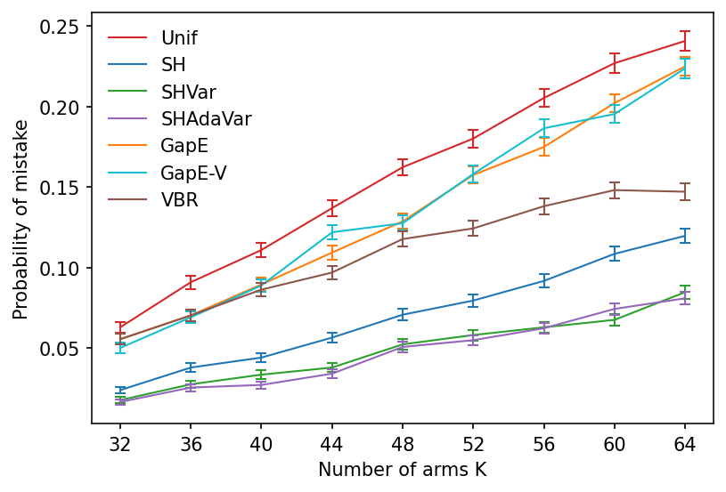
Figure 3: Probability of misidentifying the best arm in the Gaussian bandit in Section 5.1, as the number of arms $K$ increases. The budget is fixed at $n=5\,000$ and the results are averaged over $5\,000$ runs.

In the next experiment, we take same Gaussian bandit as in Figure 2. The budget is fixed at $n=5\,000$ and we vary the number of arms $K$ from $32$ to $64$. In Figure 3, we show the probability of misidentifying the best arm as the number of arms $K$ increases. We observe two major trends. First, the relative order of the algorithms, as measured by their probability of a mistake, is similar to Figure 2. Second, all algorithms get worse as the number of arms $K$ increases because the problem instance becomes harder. This experiment shows that $\tt SHVar$ and $\tt SHAdaVar$ can perform well for a wide range of $K$, they have the lowest probabilities of a mistake for all $K$. While the other algorithms perform well at $K=32$, their probability of a mistake is around $0.05$ or below; they perform poorly at $K=64$, their probability of a mistake is above $0.1$.

5.2 MovieLens Experiments

Our next experiment is motivated by the A/B testing problem in Section 1. The objective is to identify the movie with the highest mean rating from a pool of $K$ movies, where movies are arms and their ratings are rewards. The movies, users, and ratings are simulated using the MovieLens 1M dataset [Lam and Herlocker, 2016]. This dataset contains one million ratings given by $6\,040$ users to $3\,952$ movies. We complete the missing ratings using low-rank matrix factorization with rank $5$, which is done using alternating least squares [Davenport and Romberg, 2016]. The result is a $6\,040\times 3\,952$ matrix $M$, where $M_{i,j}$ is the estimated rating given by user $i$ to movie $j$.

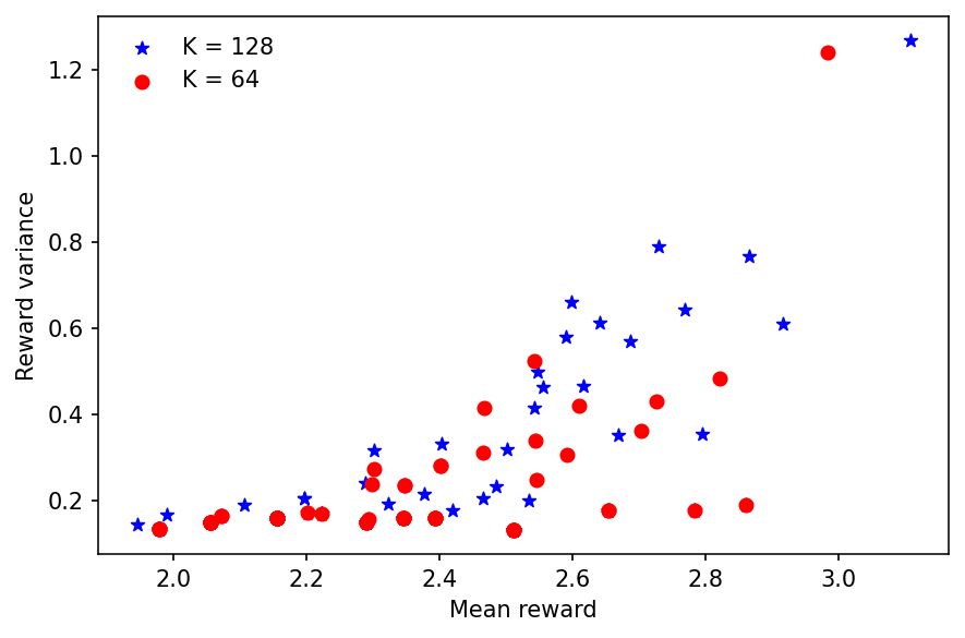
Figure 4: Means and variances of ratings of $K$ movies from the MovieLens dataset. A new sample is generated in each run of the experiment, as described in Section 5.2.

This experiment is averaged over $5\,000$ runs. In each run, we randomly choose new movies according to the following procedure. For all arms $i\in\mathcal{A}$, we generate mean $\tilde{\mu}_{i}$ and variance $\tilde{\sigma}_{i}^{2}$ as described in Section 5.1. Then, for each $i$, we find the closest movie in the MovieLens dataset with mean $\mu_{i}$ and variance $\sigma_{i}^{2}$, the movie that minimizes the distance $(\mu_{i}-\tilde{\mu}_{i})^{2}+(\sigma^{2}_{i}-\tilde{\sigma}_{i}^{2})^{2}$. The means and variances of movie ratings from two runs are shown in Figure 4. As in Section 5.1, the movies are selected so that sequential elimination with halving is expected to perform well. The variance of movie ratings in Figure 4 is intrinsic to our domain: movies are often made for specific audiences and thus can have a huge variance in their ratings. For instance, a child may not like a horror movie, while a horror enthusiast would enjoy it. Because of this, an algorithm that adapts its budget allocation to the rating variances of the remaining movies can perform better. The last notable difference from Section 5.1 is that movie ratings are realistic. In particular, when arm $i$ is pulled, we choose a random user $j$ and return $M_{j,i}$ as its stochastic reward. Therefore, this experiment showcases the robustness of our algorithms beyond Gaussian noise.

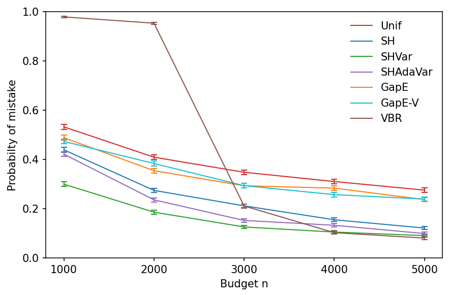
Figure 5: Probability of misidentifying the best movie in the MovieLens bandit in Section 5.2, as budget $n$ increases. The number of movies is $K=64$ and the results are averaged over $5\,000$ runs.

In Figure 5, we report the probability of misidentifying the best movie from $K=64$ as budget $n$ increases. $\tt SHVar$ and $\tt SHAdaVar$ perform the best for most budgets, although the reward distributions are not Gaussian. The relative performance of the algorithms is similar to Section 5.1: $\tt Unif$ is the worst, and $\tt GapE$ and $\tt GapE\mathchar 45\relax V$ improve upon it. The only exception is $\tt VBR$: it performs poorly for smaller budgets, and on par with $\tt SHVar$ and $\tt SHAdaVar$ for larger budgets.

We increase the number of movies next. In Figure 6, we report the probability of misidentifying the best movie from $K=128$ as budget $n$ increases. The trends are similar to $K=64$, except that $\tt VBR$ performs poorly for all budgets. This is because $\tt VBR$ has $K$ stages and eliminates one arm per stage even when the number of observations is small. In comparison, our algorithms have $\log_{2}K$ stages.

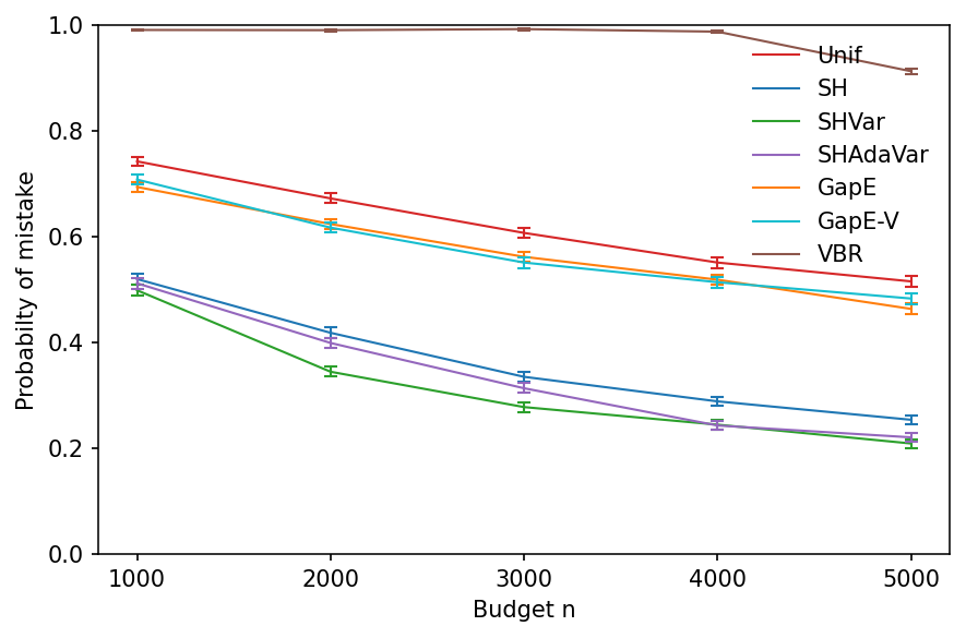
Figure 6: Probability of misidentifying the best movie in the MovieLens bandit in Section 5.2, as budget $n$ increases. The number of movies is $K=128$ and the results are averaged over $5\,000$ runs.

6 Related Work

Best-arm identification has been studied extensively in both fixed-budget [Bubeck et al., 2009, Audibert et al., 2010] and fixed-confidence [Even-Dar et al., 2006] settings. The two closest prior works are Gabillon et al. [2011] and Faella et al. [2020], both of which studied fixed-budget BAI with heterogeneous reward variances. All other works on BAI with heterogeneous reward variances are in the fixed-confidence setting [Lu et al., 2021, Zhou and Tian, 2022, Jourdan et al., 2022].

The first work on variance-adaptive BAI was in the fixed-budget setting [Gabillon et al., 2011]. This paper proposed algorithm $\tt GapE\mathchar 45\relax V$ and showed that its probability of mistake decreases exponentially with budget $n$. Our error bounds are comparable to Gabillon et al. [2011]. The main shortcoming of the analyses in Gabillon et al. [2011] is that they assume that the complexity parameter is known and used by $\tt GapE\mathchar 45\relax V$. Since the complexity parameter depends on unknown gaps and reward variances, it is typically unknown in practice. To address this issue, Gabillon et al. [2011] introduced an adaptive variant of $\tt GapE\mathchar 45\relax V$, $\tt A\mathchar 45\relax GapE\mathchar 45\relax V$, where the complexity parameter is estimated. This algorithm does not come with any guarantee.

The only other work that studied variance-adaptive fixed-budget BAI is Faella et al. [2020]. This paper proposed and analyzed a variant of successive rejects algorithm [Audibert et al., 2010]. Since $\tt SH$ of Karnin et al. [2013] has a comparable error bound to successive rejects of Audibert et al. [2010], our variance-adaptive sequential halving algorithms have comparable error bounds to variance-adaptive successive rejects of Faella et al. [2020]. Roughly speaking, all bounds can be stated as $\exp[-n/H]$, where $H$ is a complexity parameter that depends on the number of arms $K$, their variances, and their gaps.

We propose variance-adaptive sequential halving for fixed-budget BAI. Our algorithms have state-of-the-art performance in our experiments (Section 5). They are conceptually simpler than prior works [Gabillon et al., 2011, Faella et al., 2020] and can be implemented as analyzed, unlike Gabillon et al. [2011].

7 Conclusions

We study best-arm identification in the fixed-budget setting where the reward variances vary across the arms. We propose two variance-adaptive elimination algorithms for this problem: $\tt SHVar$ for known reward variances and $\tt SHAdaVar$ for unknown reward variances. Both algorithms proceed in stages and pull arms with higher reward variances more often than those with lower variances. While the design and analysis of $\tt SHVar$ are of interest, they are a stepping stone for $\tt SHAdaVar$, which adapts to unknown reward variances. The novelty in $\tt SHAdaVar$ is in solving an optimal design problem with unknown observation variances. Its analysis relies on a novel lower bound on the number of arm pulls in BAI that does not require closed-form solutions to the budget allocation problem. Our numerical simulations show that $\tt SHVar$ and $\tt SHAdaVar$ are not only theoretically sound, but also competitive with state-of-the-art baselines.

Our work leaves open several questions of interest. First, the design of $\tt SHAdaVar$ is for Gaussian reward noise. The reason for this choice is that our initial experiments showed quick concentration and also robustness to noise misspecification. Concentration of general random variables with unknown variances can be analyzed using empirical Bernstein bounds [Maurer and Pontil, 2009]. This approach was taken by Gabillon et al. [2011] and could also be applied in our setting. For now, to address the issue of Gaussian noise, we experiment with non-Gaussian noise in Section 5.2. Second, while our error bounds depend on all parameters of interest as expected, we do not provide a matching lower bound. When the reward variances are known, we believe that a lower bound can be proved by building on the work of Carpentier and Locatelli [2016]. Finally, our algorithms are not contextual, which limits their application because many bandit problems are contextual [Li et al., 2010, Wen et al., 2015, Zong et al., 2016].

Appendix A Proof of Theorem 3

First, we decompose the probability of choosing a suboptimal arm. For any $s\in[m]$, let $E_{s}=\left\{1\in\mathcal{A}_{s+1}\right\}$ be the event that the best arm is not eliminated in stage $s$ and $\bar{E}_{s}$ be its complement. Then by the law of total probability,

$$\mathbb{P}\left(\hat{I}\neq 1\right)=\mathbb{P}\left(\bar{E}_{m}\right)=\sum_{s=1}^{m}\mathbb{P}\left(\bar{E}_{s},E_{s-1}\dots,E_{1}\right)\leq\sum_{s=1}^{m}\mathbb{P}\left(\bar{E}_{s}\,\middle|\,E_{s-1}\dots,E_{1}\right)\,.$$

We bound $\mathbb{P}\left(\bar{E}_{s}\,\middle|\,E_{s-1}\dots,E_{1}\right)$ based on the observation that the best arm can be eliminated only if the estimated mean rewards of at least a half of the arms in $\mathcal{A}_{s}$ are at least as high as that of the best arm. Specifically, let $\mathcal{A}_{s}^{\prime}=\mathcal{A}_{s}\setminus\left\{1\right\}$ be the set of all arms in stage $s$ but the best arm and

$$N_{s}^{\prime}=\sum_{i\in\mathcal{A}_{s}^{\prime}}\mathds{1}\!\left\{\hat{\mu}_{s,i}\geq\hat{\mu}_{s,1}\right\}\,.$$

Then by the Markov’s inequality,

$$\mathbb{P}\left(\bar{E}_{s}\,\middle|\,E_{s-1}\dots,E_{1}\right)\leq\mathbb{P}\left(N_{s}^{\prime}\geq\frac{n_{s}}{2}\,\middle|\,E_{s-1}\dots,E_{1}\right)\leq\frac{2\,\mathbb{E}\left[N_{s}^{\prime}\,\middle|\,E_{s-1}\dots,E_{1}\right]}{n_{s}}\,.$$

The key step in bounding the above expectation is understanding the probability that any arm has a higher estimated mean reward than the best one. We bound this probability next.

Lemma 6.

For any stage $s\in[m]$ with the best arm, $1\in\mathcal{A}_{s}$, and any suboptimal arm $i\in\mathcal{A}_{s}$, we have

$$\mathbb{P}\left(\hat{\mu}_{s,i}\geq\hat{\mu}_{s,1}\right)\leq\exp\left[-\frac{n_{s}\Delta_{i}^{2}}{4\sum_{j\in\mathcal{A}_{s}}\sigma_{j}^{2}}\right]\,.$$

Proof.

The proof is based on concentration inequalities for sub-Gaussian random variables [Boucheron et al., 2013]. In particular, since $\hat{\mu}_{s,i}-\mu_{i}$ and $\hat{\mu}_{s,1}-\mu_{1}$ are sub-Gaussian with variance proxies $\sigma_{i}^{2}/N_{s,i}$ and $\sigma_{1}^{2}/N_{s,1}$, respectively; their difference is sub-Gaussian with a variance proxy $\sigma_{i}^{2}/N_{s,i}+\sigma_{1}^{2}/N_{s,1}$. It follows that

$$\mathbb{P}\left(\hat{\mu}_{s,i}\geq\hat{\mu}_{s,1}\right) =\mathbb{P}\left(\hat{\mu}_{s,i}-\hat{\mu}_{s,1}\geq 0\right)=\mathbb{P}\left((\hat{\mu}_{s,i}-\mu_{i})-(\hat{\mu}_{s,1}-\mu_{1})>\Delta_{i}\right)$$

$$\leq\exp\left[-\frac{\Delta_{i}^{2}}{2\left(\frac{\sigma_{i}^{2}}{N_{s,i}}+\frac{\sigma_{1}^{2}}{N_{s,1}}\right)}\right]=\exp\left[-\frac{n_{s}\Delta_{i}^{2}}{4\sum_{j\in\mathcal{A}_{s}}\sigma_{j}^{2}}\right]\,,$$

where the last step follows from the definitions of $N_{s,i}$ and $N_{s,1}$ in Lemma 1. ∎

The last major step is bounding $\mathbb{E}\left[N_{s}^{\prime}\,\middle|\,E_{s-1}\dots,E_{1}\right]$ with the help of Lemma 6. Starting with the union bound, we get

$$\mathbb{E}\left[N_{s}^{\prime}\,\middle|\,E_{s-1}\dots,E_{1}\right] \leq\sum_{i\in\mathcal{A}_{s}^{\prime}}\mathbb{P}\left(\hat{\mu}_{s,i}\geq\hat{\mu}_{s,1}\right)\leq\sum_{i\in\mathcal{A}_{s}^{\prime}}\exp\left[-\frac{n_{s}\Delta_{i}^{2}}{4\sum_{j\in\mathcal{A}_{s}}\sigma_{j}^{2}}\right]$$

$$\leq n_{s}\max_{i\in\mathcal{A}_{s}^{\prime}}\exp\left[-\frac{n_{s}\Delta_{i}^{2}}{4\sum_{j\in\mathcal{A}_{s}}\sigma_{j}^{2}}\right]=n_{s}\exp\left[-\frac{n_{s}\min_{i\in\mathcal{A}_{s}^{\prime}}\Delta_{i}^{2}}{4\sum_{j\in\mathcal{A}_{s}}\sigma_{j}^{2}}\right]\,.$$

Now we chain all inequalities and get

$$\mathbb{P}\left(\hat{I}\neq 1\right)\leq 2\sum_{s=1}^{m}\exp\left[-\frac{n_{s}\min_{i\in\mathcal{A}_{s}^{\prime}}\Delta_{i}^{2}}{4\sum_{j\in\mathcal{A}_{s}}\sigma_{j}^{2}}\right]\,.$$

To get the final claim, we use that

$$m=\log_{2}K\,,\quad n_{s}=\frac{n}{\log_{2}K}\,,\quad\min_{i\in\mathcal{A}_{s}^{\prime}}\Delta_{i}^{2}\geq\Delta_{\min}^{2}\,,\quad\sum_{j\in\mathcal{A}_{s}}\sigma_{j}^{2}\leq\sum_{j\in\mathcal{A}}\sigma_{j}^{2}\,.$$

This concludes the proof.

Appendix B Proof of Theorem 4

This proof has the same steps as that in Appendix A. The only difference is that $N_{s,i}$ and $N_{s,1}$ in Lemma 6 are replaced with their lower bounds, based on the following lemma.

Lemma 7.

Fix stage $s$ and arm $i\in\mathcal{A}_{s}$ in $\tt SHVar$. Then

$$N_{s,i}\geq\frac{\sigma_{i}^{2}}{\sigma_{\max}^{2}}\left(\frac{n_{s}}{\left|\mathcal{A}_{s}\right|}-1\right)\,,$$

where $\sigma_{\max}=\max_{i\in\mathcal{A}}\sigma_{i}$ is the maximum reward noise and $n_{s}$ is the budget in stage $s$.

Proof.

Let $J$ be the most pulled arm in stage $s$ and $\ell\in[n_{s}]$ be the round where arm $J$ is pulled the last time. By the design of $\tt SHVar$, since arm $J$ is pulled in round $\ell$,

$$\frac{\sigma_{J}^{2}}{N_{s,\ell,J}}\geq\frac{\sigma_{i}^{2}}{N_{s,\ell,i}}$$

holds for any arm $i\in\mathcal{A}_{s}$. This can be further rearranged as

$$N_{s,\ell,i}\geq\frac{\sigma_{i}^{2}}{\sigma_{J}^{2}}N_{s,\ell,J}\,.$$

Since arm $J$ is the most pulled arm in stage $s$ and $\ell$ is the round of its last pull,

$$N_{s,\ell,J}=N_{s,J}-1\geq\frac{n_{s}}{\left|\mathcal{A}_{s}\right|}-1\,.$$

Moreover, $N_{s,i}\geq N_{s,\ell,i}$. Now we combine all inequalities and get

$$N_{s,i}\geq\frac{\sigma_{i}^{2}}{\sigma_{J}^{2}}\left(\frac{n_{s}}{\left|\mathcal{A}_{s}\right|}-1\right)\,.$$ (8)

To eliminate dependence on random $J$, we use $\sigma_{J}\leq\sigma_{\max}$. This concludes the proof. ∎

When plugged into Lemma 6, we get

$$\mathbb{P}\left(\hat{\mu}_{s,i}\geq\hat{\mu}_{s,1}\right)\leq\exp\left[-\frac{\Delta_{i}^{2}}{2\left(\frac{\sigma_{i}^{2}}{N_{s,i}}+\frac{\sigma_{1}^{2}}{N_{s,1}}\right)}\right]\leq\exp\left[-\frac{\left(\frac{n_{s}}{\left|\mathcal{A}_{s}\right|}-1\right)\Delta_{i}^{2}}{4\sigma_{\max}^{2}}\right]\,.$$

This completes the proof.

Appendix C Proof of Theorem 5

This proof has the same steps as that in Appendix A. The main difference is that $N_{s,i}$ and $N_{s,1}$ in Lemma 6 are replaced with their lower bounds, based on the following lemma.

Lemma 8.

Fix stage $s$ and arm $i\in\mathcal{A}_{s}$ in $\tt SHAdaVar$. Then

$$N_{s,i}\geq\frac{\sigma_{i}^{2}}{\sigma_{\max}^{2}}\alpha(\left|\mathcal{A}_{s}\right|,n_{s},\delta)\left(\frac{n_{s}}{\left|\mathcal{A}_{s}\right|}-1\right)\,,$$

where $\sigma_{\max}=\max_{i\in\mathcal{A}}\sigma_{i}$ is the maximum reward noise, $n_{s}$ is the budget in stage $s$, and

$$\alpha(k,n,\delta)=\frac{1-2\sqrt{\frac{\log(1/\delta)}{n/k-2}}}{1+2\sqrt{\frac{\log(1/\delta)}{n/k-2}}+\frac{2\log(1/\delta)}{n/k-2}}$$

is an arm-independent constant.

Proof.

Let $J$ be the most pulled arm in stage $s$ and $\ell\in[n_{s}]$ be the round where arm $J$ is pulled the last time. By the design of $\tt SHAdaVar$, since arm $J$ is pulled in round $\ell$,

$$\frac{U_{s,\ell,J}}{N_{s,\ell,J}}\geq\frac{U_{s,\ell,i}}{N_{s,\ell,i}}$$

holds for any arm $i\in\mathcal{A}_{s}$. Analogously to (8), this inequality can be rearranged and loosened as

$$N_{s,i}\geq\frac{U_{s,\ell,i}}{U_{s,\ell,J}}\left(\frac{n_{s}}{\left|\mathcal{A}_{s}\right|}-1\right)\,.$$ (9)

We bound $U_{s,\ell,i}$ from below using the fact that $U_{s,\ell,i}\geq\sigma_{i}^{2}$ holds with probability at least $1-\delta$, based on the first claim in Lemma 2. To bound $U_{s,\ell,J}$, we apply the second claim in Lemma 2 to bound $\hat{\sigma}_{s,\ell,J}^{2}$ in $U_{s,\ell,J}$, and get that

$$U_{s,\ell,J}\leq\sigma_{J}^{2}\frac{1+2\sqrt{\frac{\log(1/\delta)}{N_{s,\ell,J}-1}}+\frac{2\log(1/\delta)}{N_{s,\ell,J}-1}}{1-2\sqrt{\frac{\log(1/\delta)}{N_{s,\ell,J}-1}}}$$

holds with probability at least $1-\delta$. Finally, we plug both bounds into (9) and get

$$N_{s,i}\geq\frac{\sigma_{i}^{2}}{\sigma_{J}^{2}}\frac{1-2\sqrt{\frac{\log(1/\delta)}{N_{s,\ell,J}-1}}}{1+2\sqrt{\frac{\log(1/\delta)}{N_{s,\ell,J}-1}}+\frac{2\log(1/\delta)}{N_{s,\ell,J}-1}}\left(\frac{n_{s}}{\left|\mathcal{A}_{s}\right|}-1\right)\,.$$

To eliminate dependence on random $J$, we use that $\sigma_{J}\leq\sigma_{\max}$ and $N_{s,\ell,J}\geq n_{s}/\left|\mathcal{A}_{s}\right|-1$. This yields our claim and concludes the proof of Lemma 8. ∎

Similarly to Lemma 7, this bound is asymptotically tight when all reward variances are identical. Also $\alpha(\left|\mathcal{A}_{s}\right|,n_{s},\delta)\to 1$ as $n_{s}\to\infty$. Therefore, the bound has the same shape as that in Lemma 7.

The application of Lemma 8 requires more care. Specifically, it relies on high-probability confidence intervals derived in Lemma 2, which need $N_{s,t,i}>4\log(1/\delta)+1$. This is guaranteed whenever $n\geq K\log_{2}K(4\log(1/\delta)+1)$. Moreover, since the confidence intervals need to hold in any stage $s$ and round $t$, and for any arm $i$, we need a union bound over $Kn$ events. This leads to the following claim.

Suppose that $n\geq K\log_{2}K(4\log(1/\delta)+1)$. Then, when Lemma 8 is plugged into Lemma 6, we get that

$$\mathbb{P}\left(\hat{\mu}_{s,i}\geq\hat{\mu}_{s,1}\right)\leq\exp\left[-\frac{\Delta_{i}^{2}}{2\left(\frac{\sigma_{i}^{2}}{N_{s,i}}+\frac{\sigma_{1}^{2}}{N_{s,1}}\right)}\right]\leq\exp\left[-\frac{\alpha(\left|\mathcal{A}_{s}\right|,n_{s},Kn\delta)\left(\frac{n_{s}}{\left|\mathcal{A}_{s}\right|}-1\right)\Delta_{i}^{2}}{4\sigma_{\max}^{2}}\right]\,.$$

This completes the proof.

References

- Audibert et al. [2010] Jean-Yves Audibert, Sebastien Bubeck, and Remi Munos. Best arm identification in multi-armed bandits. In Proceeding of the 23rd Annual Conference on Learning Theory, pages 41–53, 2010.
- Auer and Ortner [2010] Peter Auer and Ronald Ortner. UCB revisited: Improved regret bounds for the stochastic multi-armed bandit problem. Periodica Mathematica Hungarica, 61(1-2):55–65, 2010.
- Boucheron et al. [2013] Stephane Boucheron, Gabor Lugosi, and Pascal Massart. Concentration Inequalities: A Nonasymptotic Theory of Independence. Oxford University Press, 2013.
- Bubeck et al. [2009] Sebastien Bubeck, Remi Munos, and Gilles Stoltz. Pure exploration in multi-armed bandits problems. In Proceedings of the 20th International Conference on Algorithmic Learning Theory, pages 23–37, 2009.
- Carpentier and Locatelli [2016] Alexandra Carpentier and Andrea Locatelli. Tight (lower) bounds for the fixed budget best arm identification bandit problem. In Proceeding of the 29th Annual Conference on Learning Theory, pages 590–604, 2016.
- Davenport and Romberg [2016] Mark Davenport and Justin Romberg. An overview of low-rank matrix recovery from incomplete observations. IEEE Journal of Selected Topics in Signal Processing, 10(4):608–622, 2016.
- Even-Dar et al. [2006] Eyal Even-Dar, Shie Mannor, and Yishay Mansour. Action elimination and stopping conditions for the multi-armed bandit and reinforcement learning problems. Journal of Machine Learning Research, 7:1079–1105, 2006.
- Faella et al. [2020] Marco Faella, Alberto Finzi, and Luigi Sauro. Rapidly finding the best arm using variance. In Proceedings of the 24th European Conference on Artificial Intelligence, 2020.
- Gabillon et al. [2011] Victor Gabillon, Mohammad Ghavamzadeh, Alessandro Lazaric, and Sebastien Bubeck. Multi-bandit best arm identification. In Advances in Neural Information Processing Systems 24, 2011.
- Gabillon et al. [2012] Victor Gabillon, Mohammad Ghavamzadeh, and Alessandro Lazaric. Best arm identification: A unified approach to fixed budget and fixed confidence. In Advances in Neural Information Processing Systems 25, 2012.
- Jourdan et al. [2022] Marc Jourdan, Remy Degenne, and Emilie Kaufmann. Dealing with unknown variances in best-arm identification. CoRR, abs/2210.00974, 2022. URL https://arxiv.org/abs/2210.00974.
- Karnin et al. [2013] Zohar Karnin, Tomer Koren, and Oren Somekh. Almost optimal exploration in multi-armed bandits. In Proceedings of the 30th International Conference on Machine Learning, pages 1238–1246, 2013.
- Kaufmann et al. [2016] Emilie Kaufmann, Olivier Cappe, and Aurelien Garivier. On the complexity of best-arm identification in multi-armed bandit models. Journal of Machine Learning Research, 17(1):1–42, 2016.
- Krause et al. [2008] Andreas Krause, Ajit Paul Singh, and Carlos Guestrin. Near-optimal sensor placements in Gaussian processes: Theory, efficient algorithms and empirical studies. Journal of Machine Learning Research, 9:235–284, 2008.
- Lam and Herlocker [2016] Shyong Lam and Jon Herlocker. MovieLens Dataset. http://grouplens.org/datasets/movielens/, 2016.
- Lattimore and Szepesvari [2019] Tor Lattimore and Csaba Szepesvari. Bandit Algorithms. Cambridge University Press, 2019.
- Laurent and Massart [2000] B. Laurent and P. Massart. Adaptive estimation of a quadratic functional by model selection. The Annals of Statistics, 28(5):1302–1338, 2000.
- Li et al. [2010] Lihong Li, Wei Chu, John Langford, and Robert Schapire. A contextual-bandit approach to personalized news article recommendation. In Proceedings of the 19th International Conference on World Wide Web, 2010.
- Li et al. [2018] Lisha Li, Kevin Jamieson, Giulia DeSalvo, Afshin Rostamizadeh, and Ameet Talwalkar. Hyperband: A novel bandit-based approach to hyperparameter optimization. Journal of Machine Learning Research, 18(185):1–52, 2018.
- Lu et al. [2021] Pinyan Lu, Chao Tao, and Xiaojin Zhang. Variance-dependent best arm identification. In Proceedings of the 37th Conference on Uncertainty in Artificial Intelligence, 2021.
- Maurer and Pontil [2009] Andreas Maurer and Massimiliano Pontil. Empirical Bernstein bounds and sample-variance penalization. In Proceedings of the 22nd Annual Conference on Learning Theory, 2009.
- Pukelsheim [1993] Friedrich Pukelsheim. Optimal Design of Experiments. John Wiley & Sons, 1993.
- Soare et al. [2014] Marta Soare, Alessandro Lazaric, and Remi Munos. Best-arm identification in linear bandits. In Advances in Neural Information Processing Systems 27, pages 828–836, 2014.
- Wen et al. [2015] Zheng Wen, Branislav Kveton, and Azin Ashkan. Efficient learning in large-scale combinatorial semi-bandits. In Proceedings of the 32nd International Conference on Machine Learning, 2015.
- Zhou and Tian [2022] Ruida Zhou and Chao Tian. Approximate top- arm identification with heterogeneous reward variances. In Proceedings of the 25th International Conference on Artificial Intelligence and Statistics, 2022.
- Zong et al. [2016] Shi Zong, Hao Ni, Kenny Sung, Nan Rosemary Ke, Zheng Wen, and Branislav Kveton. Cascading bandits for large-scale recommendation problems. In Proceedings of the 32nd Conference on Uncertainty in Artificial Intelligence, 2016.