A Versatile Multi-Agent Reinforcement Learning Benchmark for Inventory Management

Abstract

Multi-agent reinforcement learning (MARL) models multiple agents that interact and learn within a shared environment. This paradigm is applicable to various industrial scenarios such as autonomous driving, quantitative trading, and inventory management. However, applying MARL to these real-world scenarios is impeded by many challenges such as scaling up, complex agent interactions, and non-stationary dynamics. To incentivize the research of MARL on these challenges, we develop MABIM (Multi-Agent Benchmark for Inventory Management) which is a multi-echelon, multi-commodity inventory management simulator that can generate versatile tasks with these different challenging properties. Based on MABIM, we evaluate the performance of classic operations research (OR) methods and popular MARL algorithms on these challenging tasks to highlight their weaknesses and potential.

1 Introduction

Reinforcement learning (RL) is a critical branch of machine learning that aims to make a sequence of optimal decisions to maximize rewards[1]. It demonstrates remarkable success in various game domains, surpassing human performance in games like Go[2], StarCraft[3, 4, 5], and DOTA2[6, 7]. Besides gaming, RL is widely used in diverse domains such as industrial production[8, 9, 10], energy control[11, 12], autonomous driving[13, 14, 15], quantitative trading[16, 17, 18], and recommendation systems[19, 20]. The RL research is closely tied to the availability of suitable environments, which is well-established in various RL fields, including Multi-Agent Particle Environment[21] and CityLearn[22] for energy control, SUMO[23] for autonomous driving, Qlib[24] for finance, and RecoGym[25] for recommendation systems.

Multi-Agent Reinforcement Learning (MARL) is a sub-field of RL that focuses on studying the behavior of multiple agents coexisting and interacting with each other in a shared environment. Due to its ability to model complex interactions and adapt to dynamic situations, MARL can be applied to real-world production scenarios where diverse and complex decisions are made simultaneously[26].

Despite its strong applicability, MARL encounters various challenges, including scaling up, agent interactions, and non-stationary contexts, among others [27]. To address these challenges, significant research efforts have been dedicated to developing solutions[28, 29, 30, 31]. However, the absence of a comprehensive benchmark makes it difficult to effectively test various algorithms on diverse challenges, and prevents a thorough evaluation of algorithm performance across an extensive range of problems.

Inventory management is a crucial aspect of Operations Research (OR), encompassing a wide range of complex real-world scenarios that require decision-making. The variety of commodities, warehouse interactions, and demand fluctuations make it an ideal platform for MARL research. To leverage this, we develop a Multi-Agent Benchmark for Inventory Management (MABIM), simulating a multi-echelon multi-agent inventory environment based on the OpenAI Gym framework[32]. MABIM captures the complexities inherent in MARL, enabling comprehensive comparisons among different MARL algorithms within a realistic production context. This benchmark promotes advancements in tackling the diverse challenges of inventory management while also providing a platform for assessing MARL algorithm performance across various tasks. The environment code is available at https://github.com/VictorYXL/ReplenishmentEnv.

Our contributions could be summarized as follows:

• We develop MABIM, an efficient and flexible inventory management environment that utilizes real data from our partner in the retail and supports multi-echelon warehouses while handling massive commodities. MABIM serves as an open and effective benchmark for addressing inventory management challenges.

• Leveraging MABIM’s flexibility, we simulate a wide range of MARL challenges, including scaling up, cooperation, competition, generalization, and robustness, further enhancing its applicability in various scenarios.

• We conduct the performance evaluation of both classic OR algorithms and MARL algorithms on these challenging scenarios, providing an in-depth analysis of their individual strengths and weaknesses.

2 Background

In this section, we start by briefly introducing the current challenges faced by MARL. Then, we present an overview of the existing MARL benchmarks. Afterwards, we introduce the inventory management problem and provide a concise summary of existing inventory management benchmarks.

MARL challenges.

MARL is a rapidly growing research field that concentrates on creating learning algorithms for multiple agents operating within a shared environment. Although it has experienced significant progress, several challenges continue to persist. These challenges involve scaling up to accommodate a large number of agents, effectively managing the intricate interactions between agents that encompass cooperation and competition, and addressing the non-stationary dynamics resulting from both environment and the interactive learning agents[27].

MARL benchmarks.

Current MARL benchmarks have certain limitations that can impede a comprehensive assessment and comparison of diverse algorithms. Table 2 compares common MARL benchmarks with ours, highlighting the maximum number of agents, dynamic contexts (or exogenous state variables, see e.g.,[33, 34]), and user customization flexibility. Previous benchmarks face challenges in accommodating scenarios with thousands of agents, incorporating dynamic contexts, and providing flexibility in a single framework. These limitations may impact the precision and applicability for evaluating MARL algorithms, underscoring the importance of developing a more comprehensive and versatile benchmark in MARL research.

Table 1: Comparison for different MARL benchmarks.

	#Agents	Interaction	Contexts	Flexibility
SMAC[35]	27	Coop.
GRF[36]	11	Coop.
GoBigger[37]	24	Coop.&Comp.		✓
MPE[38]	40	Coop.&Comp.
MA-MuJoCO[39]	6	Coop.
NeuralMMO[40]	1024	Coop.&Comp.		✓
ManiSkill[41]	2	Coop.		✓
MABIM(Ours)	2000	Coop.&Comp.	✓	✓

Table 2: Comparison for existing inventory management benchmarks.

	Real data	Multi-echelon	Multi-SKU
OR-Gym[42]		✓
MARLIM[43]	✓		✓
IM Sim.[44]	✓		✓
MABIM(Ours)	✓	✓	✓

Inventory management.

Inventory management is a critical problem in the field of operations research, involving the efficient control of the Stock Keeping Units (SKUs) for storage, acquisition, and distribution to meet customer demands and optimize costs[45]. The main objective of inventory management is to strike a balance between stock availability and storage costs while minimizing stockouts and overstocks[46]. One of the key challenges in this field is the implementation of effective replenishment strategies[47]. Effective inventory management can result in improved customer satisfaction, reduced operational costs, and enhanced overall business performance.

Classic OR algorithms are effective in specific inventory management scenarios. The base stock algorithm by Arrow et al. (1951)[48] maintains desired inventory levels by ordering when the inventory falls below a predetermined level, making it suitable for low order cost situations. Blinder et al. (1990)[49] propose the ($s,S$) algorithm to avoid frequent replenishment, triggering orders when stock falls below reorder point $s$ and replenishing to the maximum level $S$. The base stock (BS) and ($s,S$) algorithms are two popular OR algorithms and serve as baselines in our later experiments. See Appendix A for more details.

Due to the generalization and applicability of reinforcement learning algorithms, they are increasingly being applied to inventory management problems. Examples include Deep Q-Network (DQN)[50], QMIX[51], QTRAN[52], IPPO and MAPPO[53], and CD-PPO[54]. These RL algorithms demonstrate promising capabilities for addressing inventory management challenges and may provide performance improvement and better adaptability.

Inventory management benchmarks.

Despite the extensive research conducted on inventory management, there is a lack of comprehensive benchmarks in this domain. Table 2 provides an overview of existing efforts in this area. The characteristics highlighted in the table not only align the benchmark more closely with real-world production scenarios but also lend themselves to be transformed into challenges for MARL algorithms effectively.

3 MARL formulation for inventory management

In this section, we first introduce how the inventory management problem is modeled in our paper (Section 3.1), including the structure of the multi-echelon system, the dynamic process for each time step, and the calculation of the evaluation metric (i.e., the profit). Subsequently, we present the MARL formulation of this problem (Section 3.2).

3.1 Inventory management model

Multi-echelon structure.

We illustrate the multi-echelon model used in MABIM in Figure 1. This modelling is motivated by the real-world process where products are produced by the factory and transmitted through echelons of warehouses sequentially until they reach the consumers. The goal is to optimize replenishment quantities for each restocking cycle (or time step), balancing inventory to avoid overstocking (causing increasing costs) as well as understocking (causing unmet demands).

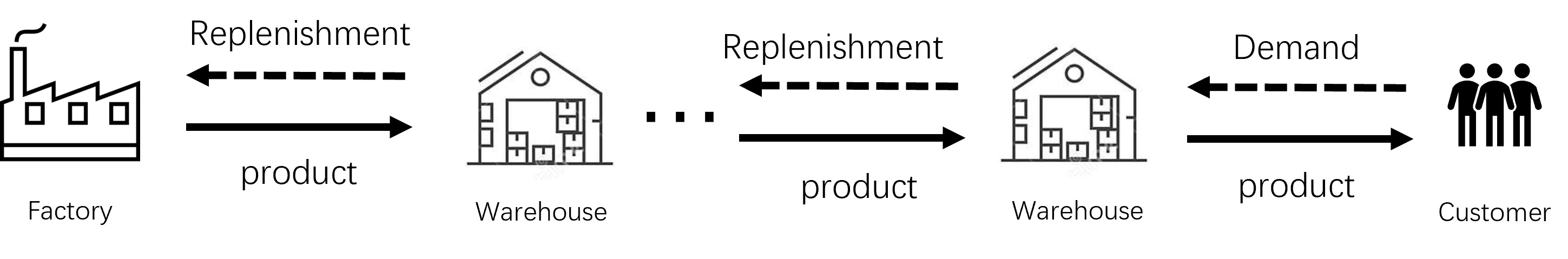
Figure 1: Multi-echelon inventory model.

Workflow.

Each time step involves the agent making decisions regarding replenishment quantities for SKUs and subsequently transitioning the environment to a new state. Let $M\in\mathbb{Z}^{+}$ be the total warehouses, with the first one being closest to customers, and $N\in\mathbb{Z}^{+}$ the total SKUs. Given a variable $X\in\{D,S,L\ldots\}$, $X_{i,j}^{t}$ represents its value for the $j$-th SKU in the $i$-th echelon at step $t$, with $0\leq i<M$ and $0\leq j<N$. Given the above notations, the main progression of a step can be described as follows:

$$D_{i+1,j}^{t+1}=R_{i,j}^{t}$$ (Replenish)

$$S_{i,j}^{t}=\min(D_{i,j}^{t},I_{i,j}^{t})$$ (Sell)

$$A_{i,j}^{t}=\sum_{k=0}^{t-1}\mathbb{I}(k+L_{i,j}^{k}==t)\cdot S_{i+1,j}^{t}$$ (Arrive)

$$\gamma_{i}^{t}=\min\left(\frac{W_{i}-\sum_{j}I_{i,j}^{t}}{\sum_{j}A_{i,j}^{t}},1\right),B_{i,j}^{t}=\lfloor A_{i,j}^{t}\cdot\gamma_{i}^{t}\rfloor$$ (Receive)

$$I_{i,j}^{t+1}=I_{i,j}^{t}-S_{i,j}^{t}+B_{i,j}^{t}$$ (Update)

Here, $D,R,S,I,A,B\in\mathbb{Z}^{+}$ and $\mathbb{I}(\text{condition})$ is an indicator function that returns 1 if the condition is true, and 0 otherwise.

• Replenish: Each warehouse requests a replenishment quantity $R$ for each SKU from the upstream source based on the policy, which becomes the demand of the upstream source. The demand $D$ with $i=0$ comes from consumers, while other demands $D$ with $i>0$ come from replenishment orders of downstream warehouses.

• Sell: Each warehouse sells the product to the downstream warehouse or consumers to meet their demands as much as possible. Specifically, the sale quantity $S$ is set to be the demand $D$ capped by the current inventory level $I$.

• Arrive: Replenished SKUs arrive after lead time $L$ steps, which may be various. Thus, SKUs replenished at different steps may arrive simultaneously, so the arrival quantity $A$ is the sum of multiple previous replenishment quantities.

• Receive: Limited warehouse capacity $W$ may prevent storing all arriving SKUs, causing overflow. The system allows custom acceptance strategies, and we present a built-in uniform receiving strategy in the above equation.

• Update: The inventory for each SKU is updated after each step.

Profit.

After each step, we calculate the profit generated by each SKU in each warehouse independently using the following formulation:

$$\text{profit}=\underbrace{p\cdot S}_{\text{Incoming}}-\underbrace{c\cdot S}_{\text{Procurement cost}}-\underbrace{v\cdot(A-B)}_{\text{Overflow cost}}-\underbrace{o\cdot\mathbb{I}(R>0)}_{\text{Order cost}}-\underbrace{h\cdot I}_{\text{Holding cost}}-\underbrace{k\cdot(D-S)}_{\text{Backlog cost}}$$ (1)

Here $p,c,v,o,h,k\in\mathbb{R}^{+}$ represent the unit selling price, procurement cost, overflow, order, holding, and backlog costs, respectively. We omit all subscripts denoting SKU, echelon, and step indices for better readability. Profit can serve as a useful metric for evaluating the effectiveness of a given strategy, and can also be used to design rewards in RL algorithm.

3.2 MARL formulation

In our formulation, each SKU in each warehouse is modelled as an agent, which is responsible for making decisions regarding its replenishment amount in a warehouse. To ensure the environment is more scalable and adaptable to various scenarios, MABIM provides built-in functions for shaping actions, rewards, and observation states. Besides, interfaces are also available to customize them easily in order to accommodate specific needs and requirements.

• The observation state for each agent is configurable, allowing for the inclusion of all current and past features of an agent. In addition to SKU features, warehouse or environment information can also be included, such as inventory occupancy and profitability.

• The action signifies the quantity of SKUs to be restocked. The system offers various built-in action-to-replenishment converters for enhanced generalization. In subsequent experiments, the average demand is used as a factor to establish the purchasing quantity.

• The reward is also configurable, with various built-in options provided. In the following experiments, we use the profit of each SKU in each warehouse as reward.

The details regarding observation state, reward, and action settings can be found in Appendix B.

4 Core features of MABIM

Building on the MARL formulation for inventory management, MABIM provides a high degree of flexibility to tackle different challenges frequently encountered in MARL research (Section 4.1). To further enhance MARL research, MABIM also offers some other features such as efficiency, ease of use, and fidelity (Section 4.2).

4.1 Tasks with configurable challenges

Compared to other inventory management environments, MABIM provides greater configuration flexibility, enabling the simulation of a wide range of challenges for MARL algorithms. This adaptability allows for customization tailored to specific use cases, enhancing the applicability of algorithms across various challenging tasks. Some typical challenges include:

• Scaling up: In the context of MARL, scaling up refers to the impact of numerous agents on training results and efficiency. While most recent MARL benchmarks do not support a large number of agents, our environment can support thousands of agents.

• Cooperation: Cooperation between agents involves collaboration between warehouses at adjacent echelons. To satisfy consumer demands, deeper cooperation is needed in longer chains. Incentives, such as product profits or backlog penalties, ensure efficient product transfer.

• Competition: Competition between agents arises when they vie for limited warehouse capacity. In our environment, reduced capacity or increased storage costs stimulate agents to compete for storage space.

• Non-stationary contexts: Non-stationary contexts present a challenge for MARL, as they require the development of algorithms capable of learning in dynamic environments with fluctuating conditions. Examples include entirely new contexts to test the algorithm’s generalization ability or noisy contexts to evaluate its robustness. These non-stationary factors may stem from external or internal sources. In the MABIM framework, the demand represents external context, and the features of SKUs serve as internal context.

The challenges mentioned above can be managed by adjusting parameters, allowing for versatile combinations. Altering parameters such as the number of SKUs, warehouses, and warehouse capacity creates challenging environments to test competition, cooperation, and scaling up, as illustrated in Figure 2.

MABIM contains a total of 51 built-in tasks with various challenges. For more details, refer to Appendix C.

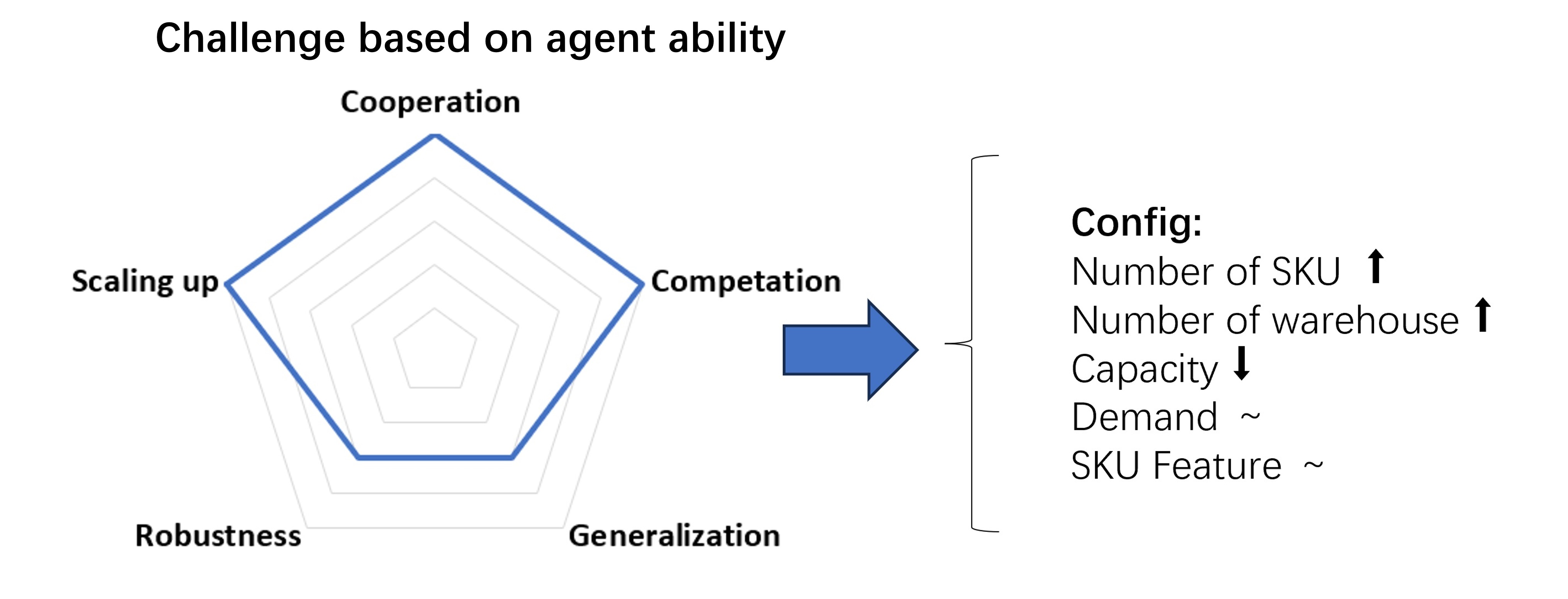
Figure 2: Combined challenge. $\uparrow$, $\downarrow$, and ~ signify increasing, decreasing, and keep steady.

4.2 Other Features

In addition to processing various challenges with configurable difficulties, MABIM possesses several noteworthy features worth mentioning.

Efficient implementation.

MABIM efficiently stores all SKU features and performs operations such as SKU initialization, purchasing, and selling in matrices. This approach ensures system efficiency and resource conservation.

Easy of use.

MABIM utilizes a unified Gym[32] interface and offers wrappers for common OR and RL algorithms. This consistency simplifies integration with other MARL frameworks and reduces the learning curve for researchers. Moreover, a visualization tool for analyzing SKU and warehouse states is provided. See Appendix D for more details.

High fidelity.

MABIM aims to simulate real-world inventory management across various aspects to ensure more applicable solutions for actual production scenarios. Key features include the use of over 2000 real demand data of SKUs, running rule-based algorithms for warmup to avoid cold starts, providing different overflow strategies for processing overflow SKUs rather than discarding them directly, and incorporating an acceptance strategy that allocates storage space based on volume ratios to ensure fairness.

5 Experiment

5.1 Experiment Settings

During experiments, we compare the performance of OR and MARL algorithms. OR algorithms include base stock (BS) and ($s,S$), and MARL algorithms include IPPO[53] and QTRAN[52]. For more details about the algorithm and hyper-parameter, see Appendix A and Appendix B.

We present an overview of the experiment settings in Table 3. In our experiments, challenging tasks are derived from a standard task that follows general inventory management logic with realistic data settings. By modifying the setting, we develop versatile challenging tasks that primarily focus on scaling up, cooperation, competition, generalization and robustness. For more details on the environment design, refer to AppendixC.

Table 3: Experiments settings. "-" means the value is the same as the standard task, "stable" refers to stable contexts from real data, "add gap" implies constant variance with random mean changes, "add noise" keeps the mean constant but adds noise to increase variance, and "#SKU * N" indicates N times the number of SKUs.

Task	#Echelon	#SKU	Capacity	Train contexts	Test contexts
Standard	1	200	#SKU * 100	Stable	Stable
Scaling up	-	$500,1000,2000$	-	-	-
Cooperation	2, 3	-	-	-	-
Competition	-	-	#SKU * 50, #SKU * 25	-	-
Generalization	-	-	-	-	Add gap
Robustness	-	-	-	Add noise	Add noise

We calculate the mean profit over all SKUs and warehouses, and then sum these mean profits over time steps to use as the evaluation metric. For the MARL algorithm, we select the best-performing model from the validation set and evaluate it on the test set. All training jobs are conducted using a single A100 graphics card.

5.2 Scaling up

We present the results for scaling up experiments in Table 4. The IPPO algorithm performs effectively when there is a small number of SKUs. However, its performance deteriorates as the number of agents increases, and it fails entirely when the number of SKUs reaches 2000. For QTRAN, although it yields good results, the training process demands significant time and GPU memory, making it resource-intensive.

Table 4: Result of scaling up tasks.

Experiment	Mean profit						Time usage		Memory usage
	BS static	BS dynamic	($s,S$) static	($s,S$) hindsight	IPPO	QTRAN	IPPO	QTRAN	IPPO	QTRAN
200 SKUs	6.29k	6.32k	8.18k	8.81k	9.83k	9.07k	11.47h	12.80h	3.15G	5.63G
500 SKUs	6.93k	7.71k	9.09k	10.13k	11.21k	11.11k	16.90h	18.15h	5.79G	11.91G
1000 SKUs	5.64k	6.37k	7.92k	8.85k	8.2k	9.44k	23.60h	34.58h	10.39G	22.61G
2000 SKUs	4.48k	5.58k	6.69k	7.97k	1.96k	8.32k	31.23h	52.28h	19.77G	44.31G

We examine the impact of scaling up on the MARL algorithm by displaying the profit on the test set during training iterations in Figure 3. As the number of SKUs increases, finding an optimal strategy for IPPO becomes more challenging, resulting in convergence failure at 2,000 agents, even after 5 million iterations. Although QTRAN exhibits better performance, it encounters substantial training instability, which could present risks in real-world applications. This highlights the difficulties associated with increasing agent numbers in the training process.

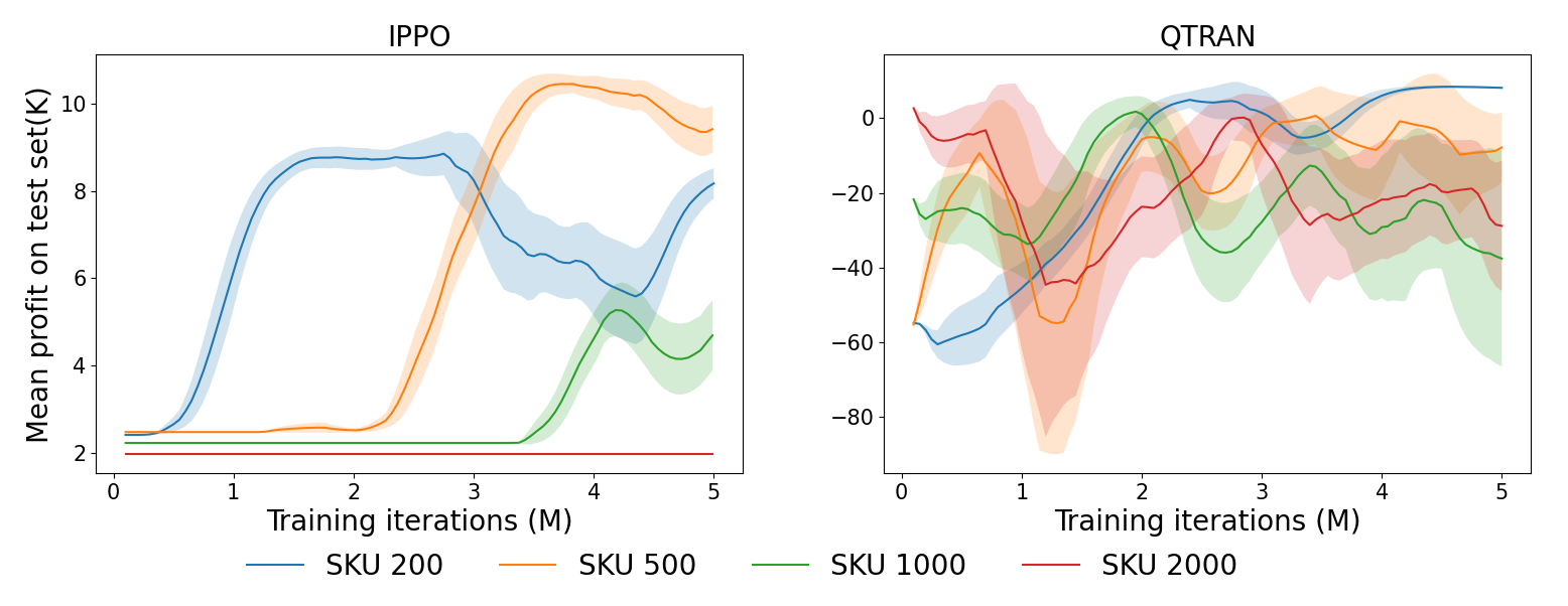
Figure 3: Mean profit in scaling up tasks.

5.3 Competition

We present the competition results in Table 5. When capacity becomes lower, competition for capacity is more incentivized, leading to a greater impact on the base stock’s static mode and the IPPO algorithm. As a result, these methods may face challenges in maintaining optimal performance under constrained capacity conditions.

Table 5: Result of competition tasks.

Experiment	BS static	BS dynamic	($s,S$) static	($s,S$) hindsight	IPPO	QTRAN
Normal capacity	6.29k	6.32k	8.18k	8.81k	9.83k	9.07k
Lower capacity	5.01k	3.64k	6.13k	7.06k	6.46k	6.74k
Lowest capacity	-7.4k	1.42k	3.32k	4.55k	-1.9k	2.04k

We analyze algorithm policies by plotting them in Figure 4. As capacity decreases, BS strategy stays unchanged since it calculates stock levels per SKU without considering overall capacity, causing overflow and higher costs. IPPO reduces replenishment quantity, potentially avoiding short-term purchases to prevent losses but not maximizing long-term profit. Both ($s,S$) static and QTRAN algorithms show better stability in performance.

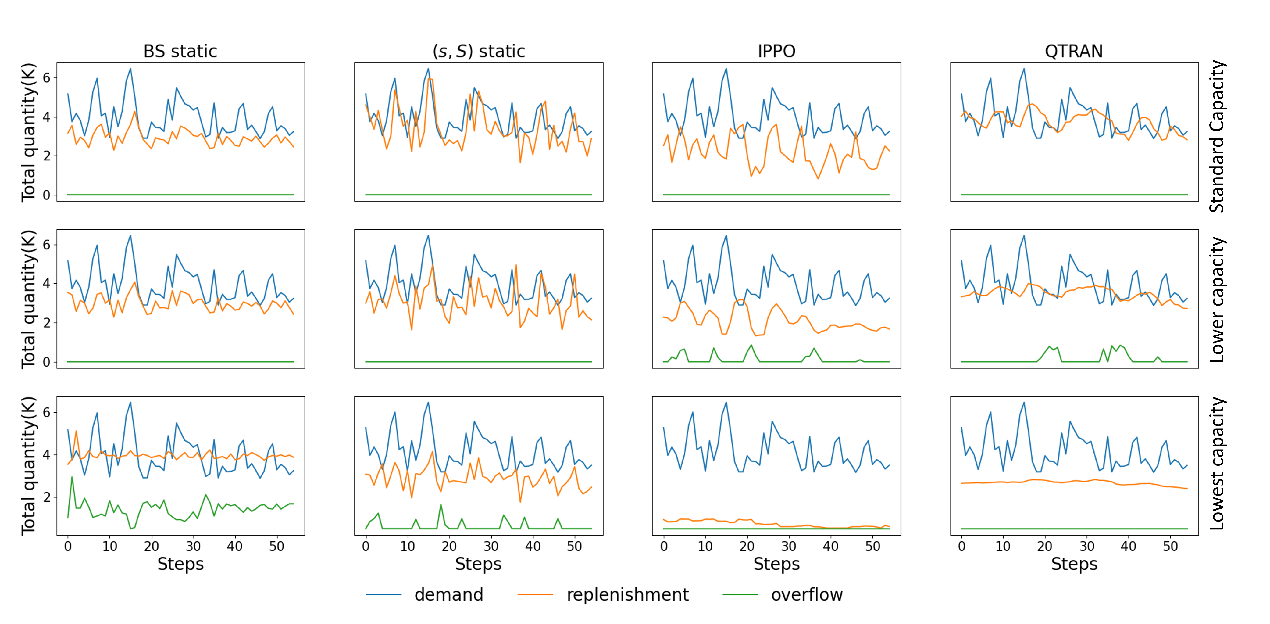
Figure 4: Policies for competition tasks. The demand, replenishment, and overflow represent the total quantity encompassing all SKUs.

5.4 Cooperation

We present the cooperation results in Table 6. To assess the collaboration between upstream and downstream operations, we design two-echelon and three-echelon inventory management models. The MARL algorithms is not as effect as in single echelon, especially IPPO. To determine if learning both upstream and downstream strategies simultaneously results in poor performance, we introduce IPPO+BS and QTRAN+BS algorithms. These algorithms utilize the IPPO/QTRAN algorithm for the upstream warehouse and the BS algorithm for warehouses in other warehouse. The combined algorithm’s performance significantly surpasses that of the pure OR and MARL algorithms. Based on these observations, we hypothesize that MARL performs well in a single warehouse, but encounters difficulties when managing both types of interactions.

Table 6: Result of cooperation tasks.

Experiment	BS static	BS dynamic	($s,S$) static	($s,S$) hindsight	IPPO	IPPO + BS	QTRAN	QTRAN + BS
Single echelon	6.29k	6.32k	8.18k	8.81k	9.83k	-	9.07k	-
2 echelons	9.15k	7.76k	9.1k	9.68k	6.72k	9.86k	9.88k	10.54k
3 echelons	8.45k	7.74k	7.92k	8.27k	4.25k	10.14k	8.09k	9.18k

We analyze algorithm policies by plotting them in Figure 5. Pure IPPO algorithm fulfill only a small demand portion. When the downstream warehouse strategy is fixed with BS, the upstream warehouse’s demand fulfillment improves, enhancing overall performance. This indicates that insufficient information exchange between upstream and downstream entities results in less effective multi-layer strategy cooperation.

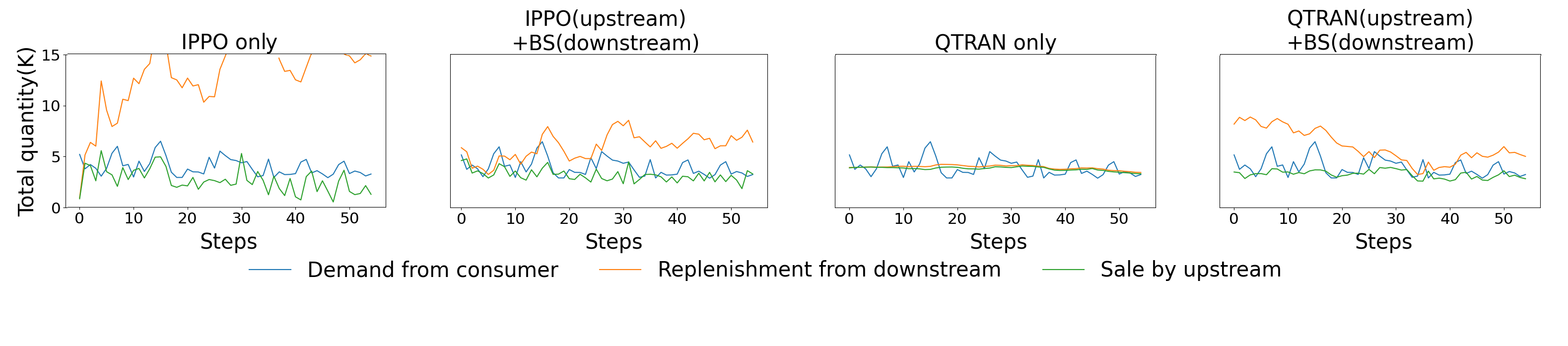
Figure 5: Policies for cooperation tasks. The demand, replenishment and sale represent the total quantity encompassing all SKUs.

5.5 Non-stationary context

In MABIM, we take into account context factors such as demand, selling price, procurement cost, lead time, and more. In this experiment, we use demand as the context and design tests to evaluate the algorithm’s capabilities for generalization and robustness. In generalization experiments, we apply an offset to test set demand, creating a new pattern unseen in training. In robustness experiments, we add random noise to demand in the entire dataset, testing the model’s ability to handle fluctuations.

As ($s,S$) hindsight algorithm directly optimizes on test data, hence is able to achieve the best performance. Its result will be used as the denominator to normalize results of other algorithms for better comparison. See Appendix E for more details on non-stationary context tasks and results.

We display the relative performance of different algorithms in Figure 6. As the gap and noise levels increase, each algorithm is impacted to varying extents. IPPO outperforms other algorithms, whereas the static OR algorithm fares the worst, particularly in generalization tasks. This result illustrates that MABIM is capable of effectively measuring the generalization and robustness of a strategy.

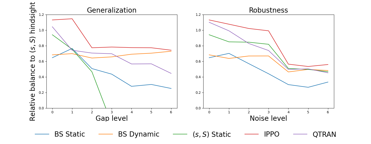
Figure 6: Relative profit of ($s,S$) hindsight.

6 Conclusion

In this paper, we introduce a MARL benchmark called MABIM, which can simulate a diverse range of challenging scenarios based on the inventory management problem. By utilizing MABIM, we develop various tasks that reveal limitations in existing MARL algorithms, such as unstable training with numerous agents, suboptimal performance under limited source, difficulties in cooperation with upstream and downstream, and the necessity for enhanced generalization and robustness. These findings highlight the importance of developing advanced MARL algorithms and demonstrate MABIM’s potential as a valuable MARL benchmark. We believe that MABIM will significantly contribute to the progress of both inventory management and MARL research.

In future work, we aim to address the issues found in MABIM and expand its capabilities to better support MARL research. Potential extensions involve constructing tree-based or graph-based inventory management structures to evaluate agent communication abilities. Additionally, we will hide some SKU features to assess the MARL algorithm performance in partially observable settings.

Appendix A OR Algorithm

In our experiment, we use 2 classical algorithms, base stock policy and ($s,S$) policy.

A.1 Base stock policy

The base stock policy is a simple and efficient inventory management strategy, in which orders are placed to replenish the inventory when the stock quantity falls below the base stock level. This policy is considered a lower bound due to its simplicity and speed. The base stock level is calculated through programming, as demonstrated in Equation A.1.

$$\begin{split}{\bf max}\quad o_{i,j}^{t}&=\bar{p}_{i,j}\cdot S_{i,j}^{t}-\bar{c}_{i,j}\cdot S_{i+1,j}^{t}-\bar{h}_{i,j}\cdot I_{i,j}^{t+1}-\bar{c}_{i,j}\cdot T_{i,j}^{0}-\bar{c}_{i,j}\cdot I_{i,j}^{0}\\ {\bf s.t}\quad I_{i,j}^{t+1}&=I_{i,j}^{t}+S_{i+1,j}^{t-\bar{L}_{i,j}}-S_{i,j}^{t}\\ \quad T_{i,j}^{t+1}&=T_{i,j}^{t}-S_{i+1,j}^{t-\bar{L}_{i,j}}+S_{i+1,j}^{t}\\ S_{i,j}^{t}&=min(I_{i,j}^{t},R_{i,j}^{t})\\ T_{i,j}^{0}&=\sum_{t=-\bar{L}_{i,j}}^{-1}S_{i+1,j}^{t}\\ z_{i,j}&=I_{i,j}^{t+1}+S_{i+1,j}^{t}+T_{i,j}^{t}\\ z_{i,j}&\in\mathbb{R^{+}}\\ \end{split}$$

In the equations mentioned above, $i$, $j$, and $t$ represent the indices of the warehouse, SKU, and time step, respectively. We also use the mean values $\bar{p}$, $\bar{c}$, $\bar{h}$, and $\bar{L}$ to denote the average selling price, procurement cost, holding cost, and lead time, respectively. The variables $S$, $R$, $I$, and $T$ represent the sale quantity, replenishment quantity, quantity in stock, and quantity in transit, respectively. Lastly, $o_{i,j}^{t}$ is the profit as the objective, and $z_{i,j}$ represents the base stock level, which is independently calculated for each product.

In the static mode, all base stock levels are calculated using historical data from the training set and consistently applied to the test set. These levels remain fixed throughout the test period. In the dynamic mode, the base stock levels are calculated using historical data and are updated at regular intervals. The levels are recalculated based on the updated historical data.

A.2 ($s,S$) Policy

The ($s,S$) policy is an effective inventory management strategy wherein orders are placed to replenish inventory when the stock quantity reaches or falls below the base reorder level, denoted as $s$. The policy aims to restore the inventory to its maximum level, represented by $S$. Due to its efficacy, the ($s,S$) policy serves as a powerful baseline, and an optimal ($s,S$) pair is sought for each SKU in the dataset. In static mode, ($s,S$) is searched in train set and in hindsight mode, ($s,S$) is searched in test set.

Appendix B MARL Algorithms

In the training process of the MARL algorithm, some implementation details include:

• The observation encompasses both SKU features and warehouse states. SKU features consist of quantity in stock, selling price, procurement cost, mean and standard deviation of historical demand, holding cost, order cost, and lead time. Warehouse states include total quantity in stock and remaining space, total profit in stock, total quantity in transit, and total profit in transit. All these features are normalized for optimal performance.

• During the training process, state and reward values are normalized using a rolling average and standard deviation. This approach enhances the model’s learning and convergence capabilities.

• For replenishment actions, we employ multiples of the average demanded quantity from the past 21 days, which ensures that inventory levels are maintained based on recent demand trends, resulting in more effective inventory management decisions.

Table 7 lists the training-related hyperparameters.

Table 7: Hyperparameters for MARL.

Hyperparameter	IPPO	QTRAN
#Epochs	5020000	5020000
Discount rate	0.985	0.985
Optimizer	Adam	Adam
Optimizer alpha	0.99	0.99
Optimizer eps	1e-5	1e-5
Learning rate	5e-4	5e-4
Grad norm clip	10	10
Horizon	21	21
Eps clip	0.15	-
Critic coef	0.5	-
Entropy coef	0	-
Accumulated episodes	1	8

Appendix C Details of Tasks Design

Standard task

The design principles behind these environment parameters ensure that more reasonable purchasing strategies yield higher benefits. A reasonable strategy encompasses the following factors:

• Most products have a purchase frequency of 2 to 10 steps.

• There is no optimal strategy for products without replenishment.

• In most cases, commodities are not purchased in excessive quantities at once (no more than 30 times the historical average daily sales volume).

• The holding and storage costs account for 10% to 25% of the gross merchandise volume (GMV) for one year, where $GMV_{i,j}=\sum_{t=1}^{365}{s_{i,j}^{t}*p_{i,j}^{t}}$.

Based on ($s,S$) policy, we search the following hyperparameter as standard configuration in Table 8. Rest feature including selling price, procurement cost, leading time are real dynamic data from external file.

Table 8: Standard configuration.

Hyperparameter	value
#SKU	200
#Warehouse	1
Capacity	20000
Order cost	10
Holding cost	0.002 + 0.001
Backlog cost	0.1 * (selling price - procurement cost)
Overflow cost	0.5 * procurement cost

Total tasks

Based on the standard task, we build-in total of 51 tasks in MABIM. Seen in Table 9

Table 9: Total tasks. "$+$" indicates the extent to which the challenge is involved.

Task name	Scaling up	Cooperation	Competition	Generalization	Robustness	More challenge
sku50.single_store.standard
sku50.2_stores.standard		$+$
sku50.3_stores.standard		$+$ $+$
sku100.single_store.standard
sku100.2_stores.standard		$+$
sku100.3_stores.standard		$+$ $+$
sku200.single_store.standard
sku200.2_stores.standard		$+$
sku200.3_stores.standard		$+$ $+$
sku500.single_store.standard
sku500.2_stores.standard	$+$	$+$
sku500.3_stores.standard	$+$	$+$ $+$
sku1000.single_store.standard
sku1000.2_stores.standard	$+$ $+$	$+$
sku1000.3_stores.standard	$+$ $+$	$+$ $+$
sku2000.single_store.standard
sku2000.2_stores.standard	$+$ $+$ $+$	$+$
sku2000.3_stores.standard	$+$ $+$ $+$	$+$ $+$
sku200.single_store.lower_capacity			$+$
sku200.single_store.lowest_capacity			$+$ $+$
sku200.2_stores.lower_capacity		$+$	$+$
sku200.2_stores.lowest_capacity		$+$	$+$ $+$
sku200.3_stores.lower_capacity		$+$ $+$	$+$
sku200.3_stores.lowest_capacity		$+$ $+$	$+$ $+$
sku200.single_store.dynamic_vlt					$+$
sku200.2_stores.dynamic_vlt		$+$			$+$
sku200.3_stores.dynamic_vlt		$+$ $+$			$+$
sku200.single_store.increase_demand				$+$	$+$
sku200.single_store.decrease_demand				$+$	$+$
sku200.single_store.higher_backlog						higher constraints
sku200.single_store.highest_backlog						highest constraints
sku200.single_store.higher_holding_cost			$+$
sku200.single_store.highest_holding_cost			$+$
sku200.single_store.higher_order_cost						lower action frequency
sku200.single_store.highest_order_cost						lowest action frequency
sku200.single_store.low_profit						low action space
sku200.single_store.high_profit						high action space
sku200.single_store.higher_overflow_cost						higher punishment
sku200.single_store.highest_overflow_cost						highest punishment
sku200.single_store.add_gap_1				$+$
sku200.single_store.add_gap_2				$+$
sku200.single_store.add_gap_3				$+$ $+$
sku200.single_store.add_gap_4				$+$ $+$
sku200.single_store.add_gap_5				$+$ $+$ $+$
sku200.single_store.add_gap_6				$+$ $+$ $+$
sku200.single_store.add_noise_1					$+$
sku200.single_store.add_noise_2					$+$
sku200.single_store.add_noise_3					$+$ $+$
sku200.single_store.add_noise_4					$+$ $+$
sku200.single_store.add_noise_5					$+$ $+$ $+$
sku200.single_store.add_noise_6					$+$ $+$ $+$

Appendix D Visualization

MABIM displays the status of each product in every warehouse during each step, along with the overall warehouse status, in the form of a webpage, as shown in Figure 7. The information provided includes demand, sales, arrivals, acceptance, replenishment, excess, inventory, items in transit, and profit, as well as procurement costs, backlog costs, order costs, and holding costs.

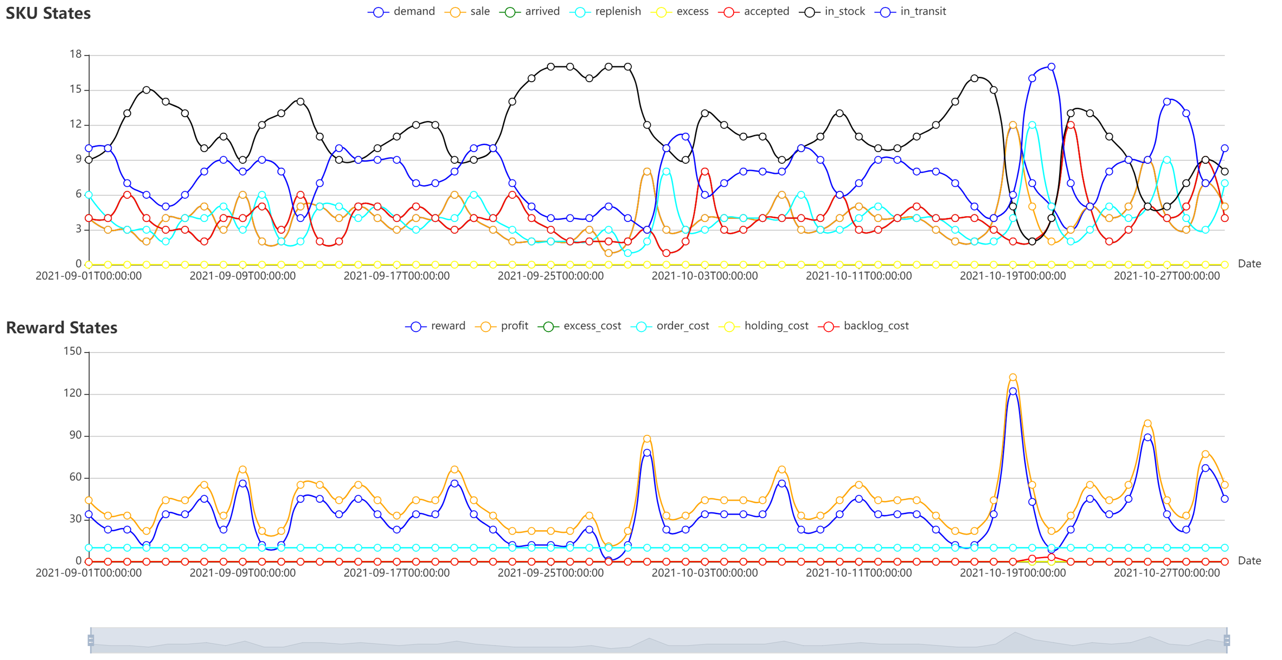
Figure 7: States of SKUs.

Appendix E Non-stationary tasks and results

Table 10: Result of non-stationary context tasks.

Experiment	Gap level	BS static	BS dynamic	($s,S$) static	($s,S$) hindsight	IPPO	QTRAN
Generalization	0 (no gap)	6.29k	6.32k	8.18k	8.81k	9.83k	9.07k
	1	4.6k	4.2k	4.54k	6.01k	6.89k	4.46k
	2	4.94k	6.26k	4.54k	9.74k	7.54k	6.88k
	3	4.31k	6.5k	-1.96k	9.89k	7.75k	6.9k
	4	4.56k	11.28k	-18.66k	16.31k	12.66k	9.24k
	5	5.69k	13.21k	-18.43k	18.74k	14.51k	10.65k
	6	5.48k	15.85k	-48.52k	21.72k	16.14k	9.68k
Experiment	Noise level	BS static	BS dynamic	($s,S$) static	($s,S$) hindsight	IPPO	QTRAN
Robustness	0(no noise)	6.29k	6.32k	8.18k	8.81k	9.83K	9.07K
	1	4.22K	3.83K	5.11K	6.01K	6.47K	5.96K
	2	4.48K	5.25K	6.64K	7.85K	8.02K	6.51K
	3	4.36K	6.62K	8.1K	9.89K	9.81K	7.31K
	4	4.92K	7.57K	8.3K	16.31K	9.2K	8.1K
	5	5.01K	9.31K	9.31K	18.74K	10.01K	9.44K
	6	7.26K	10.48K	10.14K	21.72K	12.15K	9.84k

References

- [1] Richard S Sutton and Andrew G Barto. Reinforcement Learning: An Introduction. MIT press, 2018.
- [2] David Silver, Julian Schrittwieser, Karen Simonyan, Ioannis Antonoglou, Aja Huang, Arthur Guez, Thomas Hubert, Lucas Baker, Matthew Lai, Adrian Bolton, et al. Mastering the game of go without human knowledge. Nature, 550(7676):354–359, 2017.
- [3] Oriol Vinyals, Igor Babuschkin, Wojciech M Czarnecki, Michaël Mathieu, Andrew Dudzik, Junyoung Chung, David H Choi, Richard Powell, Timo Ewalds, Petko Georgiev, et al. Grandmaster level in starcraft ii using multi-agent reinforcement learning. Nature, 575(7782):350–354, 2019.
- [4] Oriol Vinyals, Timo Ewalds, Sergey Bartunov, Petko Georgiev, Alexander Sasha Vezhnevets, Michelle Yeo, Alireza Makhzani, Heinrich Küttler, John Agapiou, Julian Schrittwieser, et al. Starcraft II: A new challenge for reinforcement learning. arXiv preprint arXiv:1708.04782, 2017.
- [5] Kun Shao, Yuanheng Zhu, and Dongbin Zhao. Starcraft micromanagement with reinforcement learning and curriculum transfer learning. IEEE Transactions on Emerging Topics in Computational Intelligence, 3(1):73–84, 2018.
- [6] Christopher Berner, Greg Brockman, Brooke Chan, Vicki Cheung, Przemysław Dębiak, Christy Dennison, David Farhi, Quirin Fischer, Shariq Hashme, Chris Hesse, et al. Dota 2 with large scale deep reinforcement learning. arXiv preprint arXiv:1912.06680, 2019.
- [7] Deheng Ye, Guibin Chen, Wen Zhang, Sheng Chen, Bo Yuan, Bo Liu, Jia Chen, Zhao Liu, Fuhao Qiu, Hongsheng Yu, et al. Towards playing full moba games with deep reinforcement learning. Advances in Neural Information Processing Systems, 33:621–632, 2020.
- [8] SPK Spielberg, RB Gopaluni, and PD Loewen. Deep reinforcement learning approaches for process control. In 2017 6th international symposium on advanced control of industrial processes, pages 201–206. IEEE, 2017.
- [9] Rui Nian, Jinfeng Liu, and Biao Huang. A review on reinforcement learning: Introduction and applications in industrial process control. Computers & Chemical Engineering, 139:106886, 2020.
- [10] Sander Adam, Lucian Busoniu, and Robert Babuska. Experience replay for real-time reinforcement learning control. IEEE Transactions on Systems, Man, and Cybernetics, Part C, 42(2):201–212, 2011.
- [11] ATD Perera and Parameswaran Kamalaruban. Applications of reinforcement learning in energy systems. Renewable and Sustainable Energy Reviews, 137:110618, 2021.
- [12] Andrew Tittaferrante and Abdulsalam Yassine. Multiadvisor reinforcement learning for multiagent multiobjective smart home energy control. IEEE Transactions on Artificial Intelligence, 3(4):581–594, 2021.
- [13] B Ravi Kiran, Ibrahim Sobh, Victor Talpaert, Patrick Mannion, Ahmad A Al Sallab, Senthil Yogamani, and Patrick Pérez. Deep reinforcement learning for autonomous driving: A survey. IEEE Transactions on Intelligent Transportation Systems, 2021.
- [14] Rui Zheng, Chunming Liu, and Qi Guo. A decision-making method for autonomous vehicles based on simulation and reinforcement learning. In 2013 International Conference on Machine Learning and Cybernetics, volume 1, pages 362–369. IEEE, 2013.
- [15] Zhenhai Gao, Tianjun Sun, and Hongwei Xiao. Decision-making method for vehicle longitudinal automatic driving based on reinforcement q-learning. International Journal of Advanced Robotic Systems, 16(3):1729881419853185, 2019.
- [16] Petter N Kolm and Gordon Ritter. Modern perspectives on reinforcement learning in finance. Modern Perspectives on Reinforcement Learning in Finance. The Journal of Machine Learning in Finance, 1(1), 2020.
- [17] Arthur Charpentier, Romuald Elie, and Carl Remlinger. Reinforcement learning in economics and finance. Computational Economics, pages 1–38, 2021.
- [18] Yuh-Jong Hu and Shang-Jen Lin. Deep reinforcement learning for optimizing finance portfolio management. In 2019 Amity International Conference on Artificial Intelligence, pages 14–20. IEEE, 2019.
- [19] Xinshi Chen, Shuang Li, Hui Li, Shaohua Jiang, Yuan Qi, and Le Song. Generative adversarial user model for reinforcement learning based recommendation system. In International Conference on Machine Learning, pages 1052–1061. PMLR, 2019.
- [20] Xueying Tang, Yunxiao Chen, Xiaoou Li, Jingchen Liu, and Zhiliang Ying. A reinforcement learning approach to personalized learning recommendation systems. British Journal of Mathematical and Statistical Psychology, 72(1):108–135, 2019.
- [21] Jayesh K Gupta, Maxim Egorov, and Mykel Kochenderfer. Cooperative multi-agent control using deep reinforcement learning. In Autonomous Agents and Multiagent Systems: AAMAS 2017 Workshops, pages 66–83. Springer, 2017.
- [22] José R Vázquez-Canteli, Jérôme Kämpf, Gregor Henze, and Zoltan Nagy. CityLearn v1.0: An OpenAI gym environment for demand response with deep reinforcement learning. In Proceedings of the 6th ACM International Conference on Systems for Energy-Efficient Buildings, Cities, and Transportation, pages 356–357, 2019.
- [23] Daniel Krajzewicz. Traffic simulation with sumo–simulation of urban mobility. Fundamentals of traffic simulation, pages 269–293, 2010.
- [24] Xiao Yang, Weiqing Liu, Dong Zhou, Jiang Bian, and Tie-Yan Liu. Qlib: An AI-oriented quantitative investment platform. arXiv preprint arXiv:2009.11189, 2020.
- [25] David Rohde, Stephen Bonner, Travis Dunlop, Flavian Vasile, and Alexandros Karatzoglou. Recogym: A reinforcement learning environment for the problem of product recommendation in online advertising. arXiv preprint arXiv:1808.00720, 2018.
- [26] Lucian Buşoniu, Robert Babuška, and Bart De Schutter. Multi-agent reinforcement learning: An overview. Innovations in multi-agent systems and applications-1, pages 183–221, 2010.
- [27] Pablo Hernandez-Leal, Bilal Kartal, and Matthew E Taylor. A survey and critique of multiagent deep reinforcement learning. Autonomous Agents and Multi-Agent Systems, 33(6):750–797, 2019.
- [28] Yaodong Yang, Rui Luo, Minne Li, Ming Zhou, Weinan Zhang, and Jun Wang. Mean field multi-agent reinforcement learning. In International conference on machine learning, pages 5571–5580. PMLR, 2018.
- [29] Jakob Foerster, Ioannis Alexandros Assael, Nando De Freitas, and Shimon Whiteson. Learning to communicate with deep multi-agent reinforcement learning. Advances in Neural Information Processing Systems, 29, 2016.
- [30] Tianshu Chu, Sandeep Chinchali, and Sachin Katti. Multi-agent reinforcement learning for networked system control. arXiv preprint arXiv:2004.01339, 2020.
- [31] Lerrel Pinto, James Davidson, Rahul Sukthankar, and Abhinav Gupta. Robust adversarial reinforcement learning. In International Conference on Machine Learning, pages 2817–2826. PMLR, 2017.
- [32] Greg Brockman, Vicki Cheung, Ludwig Pettersson, Jonas Schneider, John Schulman, Jie Tang, and Wojciech Zaremba. OpenAI Gym. arXiv preprint arXiv:1606.01540, 2016.
- [33] Thomas Dietterich, George Trimponias, and Zhitang Chen. Discovering and removing exogenous state variables and rewards for reinforcement learning. In International Conference on Machine Learning, pages 1262–1270. PMLR, 2018.
- [34] Chuheng Zhang, Yitong Duan, Xiaoyu Chen, Jianyu Chen, Jian Li, and Li Zhao. Towards generalizable reinforcement learning for trade execution. In IJCAI, 2023.
- [35] Mikayel Samvelyan, Tabish Rashid, Christian Schroeder De Witt, Gregory Farquhar, Nantas Nardelli, Tim GJ Rudner, Chia-Man Hung, Philip HS Torr, Jakob Foerster, and Shimon Whiteson. The starcraft multi-agent challenge. arXiv preprint arXiv:1902.04043, 2019.
- [36] Karol Kurach, Anton Raichuk, Piotr Stańczyk, Michał Zając, Olivier Bachem, Lasse Espeholt, Carlos Riquelme, Damien Vincent, Marcin Michalski, Olivier Bousquet, et al. Google research football: A novel reinforcement learning environment. In Proceedings of the AAAI Conference on Artificial Intelligence, volume 34, pages 4501–4510, 2020.
- [37] Ming Zhang, Shenghan Zhang, Zhenjie Yang, Lekai Chen, Jinliang Zheng, Chao Yang, Chuming Li, Hang Zhou, Yazhe Niu, and Yu Liu. Gobigger: A scalable platform for cooperative-competitive multi-agent interactive simulation. In The Eleventh International Conference on Learning Representations, 2023.
- [38] Igor Mordatch and Pieter Abbeel. Emergence of grounded compositional language in multi-agent populations. In Proceedings of the AAAI conference on artificial intelligence, volume 32, 2018.
- [39] Bei Peng, Tabish Rashid, Christian Schroeder de Witt, Pierre-Alexandre Kamienny, Philip Torr, Wendelin Böhmer, and Shimon Whiteson. Facmac: Factored multi-agent centralised policy gradients. Advances in Neural Information Processing Systems, 34:12208–12221, 2021.
- [40] David Ha and Yujin Tang. Collective intelligence for deep learning: A survey of recent developments. Collective Intelligence, 1(1):26339137221114874, 2022.
- [41] Tongzhou Mu, Zhan Ling, Fanbo Xiang, Derek Yang, Xuanlin Li, Stone Tao, Zhiao Huang, Zhiwei Jia, and Hao Su. Maniskill: Generalizable manipulation skill benchmark with large-scale demonstrations. arXiv preprint arXiv:2107.14483, 2021.
- [42] Christian D Hubbs, Hector D Perez, Owais Sarwar, Nikolaos V Sahinidis, Ignacio E Grossmann, and John M Wassick. Or-gym: A reinforcement learning library for operations research problems. arXiv preprint arXiv:2008.06319, 2020.
- [43] Leluc Remi, Kadoche Elie, Bertoncello Antoine, and Gourv enec Sebastien. Marlim: Multi-agent reinforcement learning for inventory management. Advances in Neural Information Processing RL4RealLife Workshop, 2022.
- [44] Puppala Sridhar, CR Vishnu, and R Sridharan. Simulation of inventory management systems in retail stores: A case study. Materials Today: Proceedings, 47:5130–5134, 2021.
- [45] Sridhar Tayur, Ram Ganeshan, and Michael Magazine. Quantitative models for supply chain management, volume 17. Springer Science & Business Media, 2012.
- [46] John W Toomey. Inventory management: principles, concepts and techniques, volume 12. Springer Science & Business Media, 2000.
- [47] Hartmut Stadtler. Supply chain management: An overview. Supply chain management and advanced planning: Concepts, models, software, and case studies, pages 3–28, 2014.
- [48] Kenneth J Arrow, Theodore Harris, and Jacob Marschak. Optimal inventory policy. Econometrica: Journal of the Econometric Society, pages 250–272, 1951.
- [49] Alan S Blinder. Inventory theory and consumer behavior. Harvester Wheatsheaf, 1990.
- [50] M-A Dittrich and S Fohlmeister. A deep q-learning-based optimization of the inventory control in a linear process chain. Production Engineering, 15:35–43, 2021.
- [51] Tabish Rashid, Mikayel Samvelyan, Christian Schroeder De Witt, Gregory Farquhar, Jakob Foerster, and Shimon Whiteson. Monotonic value function factorisation for deep multi-agent reinforcement learning. The Journal of Machine Learning Research, 21(1):7234–7284, 2020.
- [52] Kyunghwan Son, Daewoo Kim, Wan Ju Kang, David Earl Hostallero, and Yung Yi. Qtran: Learning to factorize with transformation for cooperative multi-agent reinforcement learning. In International conference on machine learning, pages 5887–5896. PMLR, 2019.
- [53] Y. Zheng, X. Chen, J. Wang, and M. Chen. A deep reinforcement learning approach for inventory management in retail. Industrial Management & Data Systems, 2020.
- [54] Yuandong Ding, Mingxiao Feng, Guozi Liu, Wei Jiang, Chuheng Zhang, Li Zhao, Lei Song, Houqiang Li, Yan Jin, and Jiang Bian. Multi-agent reinforcement learning with shared resources for inventory management. In Advances in Neural Information Processing RL4RealLife Workshop, 2022.