Learning Unnormalized Statistical Models via Compositional Optimization
Abstract
Learning unnormalized statistical models (e.g., energy-based models) is computationally challenging due to the complexity of handling the partition function. To eschew this complexity, noise-contrastive estimation (NCE) has been proposed by formulating the objective as the logistic loss of the real data and the artificial noise. However, as found in previous works, NCE may perform poorly in many tasks due to its flat loss landscape and slow convergence. In this paper, we study a direct approach for optimizing the negative log-likelihood of unnormalized models from the perspective of compositional optimization. To tackle the partition function, a noise distribution is introduced such that the log partition function can be written as a compositional function whose inner function can be estimated with stochastic samples. Hence, the objective can be optimized by stochastic compositional optimization algorithms. Despite being a simple method, we demonstrate that it is more favorable than NCE by (1) establishing a fast convergence rate and quantifying its dependence on the noise distribution through the variance of stochastic estimators; (2) developing better results for one-dimensional Gaussian mean estimation by showing our objective has a much favorable loss landscape and hence our method enjoys faster convergence; (3) demonstrating better performance on multiple applications, including density estimation, out-of-distribution detection, and real image generation.
1 Introduction
We investigate the problem of learning unnormalized statistical models. Suppose we observe a set of training samples from an unknown probability density function (pdf) and estimate this data pdf by
| (1) |
where is defined as an unnormalized model, and denotes the parameter that will be learnt to best fit the data. The term in equation (1) is called partition function, which is used to ensure the final model is normalized, i.e., . By introducing the partition function, we can use more flexible structures to represent . Specifically, if we set , the above formulation (1) reduces to the well-known energy-based model (EBM) (LeCun et al., 2006):
which enjoys wide applications in machine learning (Du & Mordatch, 2019; Yu et al., 2020; Grathwohl et al., 2020a).
To find the best parameter for the given model , we can directly maximize the log-likelihood on the observed training data, i.e., optimizing the objective , where
| (2) |
However, the challenge is that the log partition function and its gradient are difficult to calculate exactly. To remedy this issue, prior works (Hinton, 2002; Tieleman, 2008; Nijkamp et al., 2019a) resort to Markov chain Monte Carlo (MCMC) sampling (Christian P. Robert, 2004). Considering the gradient of loss , we have:
where denotes the pdf . To compute the second term, previous literature applies a number of MCMC steps to sample from , and then calculates the estimated gradient. However, MCMC sampling is slow and unstable during training (Grathwohl et al., 2020b; Ruiqi et al., 2020; Geng et al., 2021), partly because approximate samples are obtained with only a finite number of steps. As pointed out by Nijkamp et al. (2019b) and Grathwohl et al. (2020b), estimating with finite MCMC steps will produce biased estimations, leading to optimizing a different objective other than the original MLE loss.
To eschew the complexity of estimating the gradient of log partition function, noise-contrastive estimation (NCE) (Gutmann & Hyvärinen, 2012) has been proposed, which transforms the original problem into a classification task. Specifically, NCE introduces a noise distribution , and then optimizes the extended model parameter by minimizing the following loss:
where , and the parameter is used to estimate the log partition function, i.e., . This new objective can be interpreted as the logistic loss to distinguish between the noise and the real data. In practice, the first term is estimated by observed training examples and the second term is evaluated by noise samples where .
However, as pointed out in many works (Goodfellow et al., 2014; Ruiqi et al., 2020), if the noise distribution is very different from the data distribution , this classification problem would be too easy to solve and the learned model may fail to capture adequate information about the real data distribution. In particular, Liu et al. (2022a) demonstrate that when and are not close enough, the loss is extremely flat near the optimum, leading to the slow convergence rate of NCE method.
In this paper, we investigate an alternative approach for directly optimizing the MLE objective by converting it to a stochastic compositional optimization (SCO) problem. To deal with the intractable partition function, we introduce a noise distribution , and then convert the log partition function into . Then, the objective function (2) becomes:
which can be written as a two-level SCO problem. Since SCO has been studied extensively, state-of-the-art algorithms can be employed to solve the above problem. However, besides its simplicity, a major question remains: What are the advantages of this approach compared with NCE and MCMC-based methods for learning unnormalized models? Our main contributions are to demonstrate the following advantages by theoretical analysis and empirical studies:
-
1.
We prove that our single-loop algorithm converges asymptotically to an optimal solution under the Polyak-Łojasiewicz (PL) condition, and establish a fast convergence rate in the order of for finding an -optimal solution. In contrast, NCE and MCMC-based approaches do not provide such guarantees.
-
2.
We prove through one-dimensional Gaussian mean estimation that the MLE objective function has a better loss landscape than the NCE objective, and establish a faster convergence rate of our algorithm than a state-of-the-art NCE-based approach (Liu et al., 2022a) for this task.
-
3.
We illustrate the better performance of our method on different tasks, namely, density estimation, out-of-distribution detection, and real image generation. For the last task, we show that the choice of the noise distribution has a significant impact on the quality of generated data in line with our theoretical analysis.
2 Related Work
This section reviews related work on noise contrastive estimation, and other methods for learning unnormalized models, as well as stochastic compositional optimization.
2.1 Noise-contrastive Estimation
Noise-contrastive estimation (NCE) is first proposed by Gutmann & Hyvärinen (2010, 2012), and gains its popularity in machine learning applications quickly (Mnih & Kavukcuoglu, 2013; Hjelm et al., 2019; Henaff, 2020; Tian et al., 2020; Kong et al., 2020). The basic idea is to introduce a noise distribution, and then distinguish it from the data distribution by a logistic loss. As pointed out in previous works (Goodfellow et al., 2014; Ruiqi et al., 2020; Liu et al., 2022a), the choice of the noise distribution is crucial to the success of NCE, and many methods have been proposed to tune the noise automatically. For example, Bose et al. (2018) utilize a learned adversarial distribution as the noise, and develop a method named Adversarial Contrastive Estimation. At the same time, Conditional NCE is introduced by Ceylan & Gutmann (2018), which generates the noise samples with the help of the observed data. Afterward, Ruiqi et al. (2020) propose Flow Contrastive Estimation, using a flow model to learn the noise distribution by joint training. However, these methods usually introduce extra computation, and the adversarial training of the noise is slow and complex. Instead of designing more complicated noise, Liu et al. (2022a) recently propose a new objective named eNCE, which replaces the log loss in NCE as the exponential loss, and enjoys better results for exponential families. However, eNCE still suffers from the ill-behaved loss landscape, which is extremely flat near the optimum.
2.2 Other Methods for Learning Unnormalized Models
Except NCE and its variants discussed above, there are also many other approaches to solve unnormalized models. To bypass the partition function, score matching (Hyvärinen, 2005) optimizes the squared distance between the gradient of the log density of the model and that of the observed data, in which the partition function would not appear. However, the output dimension of score matching is the same as the input, and training such a model is expensive and unstable, especially for high-dimensional data (Song & Ermon, 2019; Pang et al., 2020). Existing works usually require denoising (Vincent, 2011) or slicing (Song et al., 2019) techniques to train score matching methods.
Besides NCE and score matching, optimizing MLE objective with Markov chain Monte Carlo (MCMC) sampling is also widely used. One well-known method is Contrastive Divergence (CD) introduced by Hinton (2002), which employs MCMC sampling for fixed steps. To sample more efficiently, Tieleman (2008) initializes the MCMC in each training step with the previous sampling results and names this method as persistent CD. Other variants of CD have also been proposed later, such as modified CD (Gao et al., 2018), adversarial CD (Han et al., 2019), etc. These techniques are also very popular in learning energy-based models (EBM), which is a special case of unnormalized models. Specifically, Xie et al. (2016) propose to learn EBM by using ConvNet as the energy function; then, Xie et al. (2018) and Jianwen et al. (2018) use a generator as a fast sampler to help EBM training. Note that the objective of the EBM becomes a modified contrastive divergence, and Xie et al. (2021) and Xie et al. (2022) are proposed as different variants of Jianwen et al. (2018), whose objectives are also a modified contrastive divergence. However, the main drawback of these methods is that MCMC sampling is usually time-consuming and unstable during training (Grathwohl et al., 2020b; Ruiqi et al., 2020; Geng et al., 2021).
2.3 Stochastic Compositional Optimization
Stochastic Compositional Optimization (SCO) has been investigated extensively in the literature. The objective of a two-level SCO is given by , where and are random variables. To solve this problem, Wang et al. (2017a) develop stochastic compositional gradient descent (SCGD), which achieves a complexity of , , and for non-convex, convex, and -strongly convex functions, respectively. These complexities are further improved to , and in a subsequent work (Wang et al., 2017b).
To obtain a better rate, Ghadimi et al. (2020) propose a method named averaged stochastic approximation (NASA), which uses momentum-update to estimate the inner function and the gradient, and attains a complexity of for non-convex objectives. Recently, with the popularity of variance reduction methods such as SARAH (Nguyen et al., 2017), SPIDER (Fang et al., 2018) and STORM (Cutkosky & Orabona, 2019), this complexity is further improved to , by estimating the inner function and the gradient with variance-reduction techniques (Zhang & Xiao, 2019; Chen et al., 2021; Qi et al., 2021a).
3 The Proposed Method
In this section, we propose to learn unnormalized models directly by Maximum likelihood Estimation via Compositional Optimization (MECO). First, it is easy to show that, with a noise distribution , the MLE objective function (2) is equivalent to:
However, optimizing this objective is nontrivial, because of the nested structure of the second term. Specifically, we can not acquire its unbiased estimation by sampling from , since the expectation cannot be moved out of the log function, i.e., . Due to similar reasons, we also can not obtain an unbiased estimation of its gradient, which is the main obstacle to deriving an algorithm with convergence guarantees.
To solve this difficulty, we can treat the as a compositional function, where is the outer function and is the inner function, which can be unbiased-estimated by sampling form . Inspired by NASA (Ghadimi et al., 2020) for solving stochastic compositional optimization (SCO), we use variance reduced estimators to approximate the inner function and the gradient, so that the estimation errors can be reduced over time. Specifically, considering the gradient of the objective function w.r.t. parameter , we have:
To estimate this gradient, in each training step , we first draw sample from the training set , and sample from the noise distribution . Then, we estimate by a function value estimator in the style of momentum update:
| (3) |
When evaluating the gradient, we would use to approximate the term in the denominator. Similarly, we employ a gradient estimator to track the overall gradient by another momentum update:
| (4) | ||||
Although the estimators and are still biased, it can be proved that the estimation error is reduced gradually. After obtaining the gradient estimator , we use it to update the parameter in the style of SGD. The whole algorithm is presented in Algorithm 1. Note that in the first iteration, we can simply set the estimator and .
Difference from NASA: The optimization method we used can be viewed as a modified version of NASA for SCO problems (Ghadimi et al., 2020). Compared with the original NASA applied to constrained SCO, our method does not need to project the variable onto the feasible set and is thus simpler. Another big difference from NASA lies in the improved rate we will derive for an objective satisfying the PL condition, which is missing in their original work.
Difference from energy-based model (EBM) training: Derived from SCO, our algorithm has a key difference from the standard EBM training. By setting , the unnormalized model converts to the EBM, and our gradient estimator is written as:
In contrast, EBM usually optimizes the objective function , and its stochastic gradient is written as . In this sense, our method can be viewed as introducing an adaptive weight to the second term and applying SGD with momentum to update the model.
4 Theoretical Analysis
We first present the advantage of the MLE formulation, and then analyze the convergence rate of the proposed method, as well as its relationship with the noise distribution. Due to space limitations, all the proofs are deferred to the appendix.
4.1 Advantages of the MLE Formulation
Since we use MLE to optimize unnormalized models, our objective inherits several nice properties. Here, we analyze the behavior of the estimator for large sample sizes and assume that there exists an optimal solution such that . To compare different estimators, we introduce the definition of asymptotic relative efficiency (ARE) (Vaart, 1998) below.
Definition 1.
For any two estimators and with
the ARE of to is defined by .
Remark: From the definition, we know that indicates estimator is more efficient than estimator .
Theorem 1.
According to the property of MLE (Wasserman, 2004), the estimator enjoys the following guarantees:
-
1.
(Consistent) The estimator converges in probability to , i.e., .
-
2.
(Asymptotically Normal) , where can be computed analytically.
-
3.
(Asymptotically Optimal) Denote that is the output of any other estimator, then .
Remark: The last property implies that the MLE objective has the smallest variance, indicating it is better than optimizing other objectives, e.g., the NCE objective.
4.2 The Convergence of the Proposed Method
Then, we analyze the convergence of Algorithm 1. First, we define the sample complexity to measure the convergence rate, which is widely used in stochastic optimization.
Definition 2.
The sample complexity is the number of samples needed to find a point satisfying (-stationary), or (-optimal).
For notation simplicity, we denote , , , estimator and , where and are samples drawn from and .
Next, we make the following assumptions, which are commonly used in SCO problems (Wang et al., 2016; Zhang & Xiao, 2019, 2021; Wang & Yang, 2022; Jiang et al., 2022b).
Assumption 1.
We assume that (i) function , are Lipchitz continuous and smooth with respect to their inputs, is a smooth function; (ii) is lower bounded by .
Assumption 2.
There exist such that
Remark: In Assumption 1, is Lipchitz and smooth in terms of its input when , where is a positive constant. Assumption 2 assumes that the variances of estimating , and by sampling from the corresponding distributions are bounded.
We first derive an asymptotic convergence result, showing that Algorithm 1 can converge to a stationary point of .
Theorem 2.
Assume that the sequence of stepsizes satisfies . Then with probability 1, accumulation point ,, of the sequence ,, generated by Algorithm 1 satisfies:
Next, we present the non-asymptotic convergence result.
Theorem 3.
For non-convex function , by setting , , Algorithm 1 finds an -stationary point in iterations.
Remark: The analysis of above two theorems closely follows Ghadimi et al. (2020).
The main contribution of our analysis is to show that by properly setting the hyper-parameters, Algorithm 1 can enjoy a faster convergence rate when the objective satisfies the Polyak-Łojasiewicz (PL) condition (Karimi et al., 2016). We give the definition of the PL condition below.
Definition 3.
satisfies the -PL condition if there exists such that .
Remark: PL condition has been shown to be satisfied for deep learning under over-parameterized networks by many prior works (Allen-Zhu et al., 2019; Du et al., 2019). Under the PL condition, a stationary point becomes a global optimal solution of objective . Thus, our algorithm asymptotically converges to an optimal solution according to Theorem 2. Next, we show the improved complexity under the PL condition as stated below.
Theorem 4.
When the objective satisfies -PL condition, by setting and , Algorithm 1 can find an -optimal solution in iterations.
Remark: We emphasize that the above convergence for a single-loop algorithm is novel in SCO. Existing methods for SCO usually have to employ two-loop stagewise methods to obtain similar results under the PL condition (Zhang & Xiao, 2019; Qi et al., 2021b; Jiang et al., 2022b).
4.3 Choosing the Noise Distribution
Similar to NCE, our approach also relies on a noise distribution . The difference is that the noise distribution only affects the convergence rate of our method, not the optimal solution. Theorem 2 shows that our algorithm will eventually converge to a stationary point or a global optimal solution (under PL condition) of the MLE objective, as long as is positive whenever is positive, no matter what the noise distribution is. On the other hand, the noise distribution would affect the objective function of NCE, and it is pointed out that if the noise distribution is too different from data distribution, the classification problem becomes too easy, which prevents the model from learning much about the data structure (Gutmann & Hyvärinen, 2012). For our method, the impact of on the convergence rate is through the variance of and . From our theoretical results (Theorems 3 and 4), we can see that if the variance is zero, then the noise distribution has no impact on the convergence rate. We show the condition to satisfy the zero variance below.
Lemma 1.
If , then and .
Remark: However, the above choice is impractical as sampling from is not easy, and the dependence of on would also make our convergence analysis fail. In practice, we can only hope is close to .
Also, to ensure the partition function can be written as , we should guarantee whenever . This is also required in NCE, which is not difficult to satisfy, since many continuous probability distributions can ensure their probability density functions are always positive, e.g., Gaussian, Laplace and Cauchy distributions. Thus, our analysis suggests the following:
-
1.
Choose that can be easily sampled and computed.
-
2.
We should ensure whenever .
-
3.
The noise distribution should be similar to or the data distribution .
To satisfy the last two properties, we can sample the real data and add some noise to the data. In particular, to sample , we first sample , , and then set . Since and denote the probability density function of by , the noise distribution would be , which can be approximated within the mini-batch in practice. To ensure that the noise is similar to the data, we can also fit the parameter and by some training data, which can be easily done by using the existing numpy package via numpy.mean() and numpy.cov(). In our empirical study, this is helpful for high-dimensional problems, i.e., image generation on MNIST data set in Section 6.3. For simple problems, such as density estimation and out-of-distribution detection, we can simply set the noise as a multivariate Gaussian distribution, which is very fast and easy to sample from. Since more complex noise would introduce more computations, it is a trade-off in practice.
Finally, we would like to emphasize that the impact of the noise distribution can be alleviated by increasing the mini-batch size for estimating and . If the mini-batch size of noisy samples is , then the variance and will be scaled by . Hence, the larger the batch size, the less impact of the noise distribution on the convergence rate.
5 Case Study: Gaussian Mean Estimation
As pointed out by Liu et al. (2022a), the reason that NCE may fail to learn a good parameter is due to its flat loss landscape. To verify this claim, they use one-dimensional Gaussian mean estimation as an example and show the slow convergence of NCE for this simple task. To demonstrate the effectiveness of our method, we use the same task to show the behavior of our loss and the proposed optimization method. Following their setup, the data and noise distributions are Gaussian distributions with mean and separately, and the variances are both fixed as 1, i.e.,
Then, assume that the model is another Gaussian distribution with mean and variance 1, which is equivalent to setting . The goal is to learn the parameter , or for NCE. First, we can see the flatness of NCE loss via the proposition below.
Proposition 1.
(Proposition 4.2 in Liu et al. (2022a))
Denote that and is the NCE loss. Then, we have , where is the optimal solution.
Remark: If and are not close enough, the difference between and will be extremely small when approaches , implying a flat landscape.
However, it is not a problem for the MLE objective that we optimize, which is shown in the following proposition.
Proposition 2.
For -d Gaussian mean estimation, the MLE objective satisfies that .
Remark: Compared with NCE, the MLE objective does not have the extremely small factor , and thus has a much better loss landscape near the optimum.
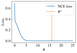
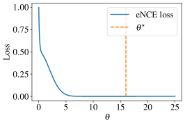
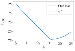
To show this difference more vividly, we plot the loss landscape of the NCE objective and the MLE objective, as well as the newly proposed eNCE objective (Liu et al., 2022a). Following the same setup as Liu et al. (2022a), we set and . The results are shown in Figure 1. As can be seen, both the NCE and eNCE objectives are very flat near the optimal solution, while the MLE objective is very sharp.
Besides, we provide the convergence rate of our method for this task, as stated below.
Proposition 3.
For 1- Gaussian mean estimation, Algorithm 1 ensures after iterations.
Remark: Although Liu et al. (2022a) can ensure that after iterations, by using normalized gradient descent (NGD) for the NCE or eNCE objective, their assumptions are very strong. They assume the algorithm can obtain the exact gradient, which is impossible in practice. In contrast, our analysis only relies on stochastic gradients. Also note that NCE optimized with standard gradient descent requires an exponential number of steps to find a reasonable parameter, according to Liu et al. (2022a).
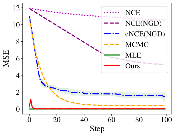
Finally, we conduct experiments to compare different methods. We choose mean square error (MSE) as the criterion and compare our method with NCE trained by SGD and NGD, MCMC training (Du & Mordatch, 2019), and the eNCE objective trained by NGD. The results are presented in Figure 2, which demonstrate that our method converges more quickly than other methods, and NCE is the slowest due to its flat loss landscape. Since MLE can be calculated for Gaussian distribution directly, we also include a curve for MLE as a reference, which is very close to the curve of our method after a few steps. Note that we run each method for 100 steps, and we report the running time of each method in Table 1, It can be seen that the running time of NCE and our method are very similar, while the MCMC method is much slower. As a result, it is fair to compare the convergence between NCE and our method.
| NCE | NCE (NGD) | eNCE (NGD) | MCMC | Ours |
| 176s | 181s | 169s | 1757s | 168s |
| Method | 2spirals | 8gaussians | checkerboard | circles | moons | swissroll |
| NCE | 3.253 ± 0.284 | 0.153 ± 0.095 | 1.956 ± 0.469 | 1.223 ± 0.154 | 5.178 ± 0.341 | 2.715 ± 0.249 |
| NCE (NGD) | 3.445 ± 0.287 | 0.177 ± 0.102 | 1.963 ± 0.488 | 1.270 ± 0.292 | 5.010 ± 0.349 | 2.585 ± 0.201 |
| eNCE (NGD) | 3.328 ± 0.332 | 0.257 ± 0.144 | 1.810 ± 0.218 | 1.183± 0.188 | 4.728 ± 0.399 | 2.975 ± 0.398 |
| MCMC | 3.060 ± 0.780 | 0.150 ± 0.035 | 1.654 ± 0.217 | 1.154 ± 0.294 | 4.722 ± 0.633 | 2.764 ± 0.670 |
| Score Matching | 3.268 ± 0.846 | 0.250 ± 0.076 | 2.167 ± 0.703 | 1.302 ± 0.272 | 4.826 ± 0.153 | 2.660 ± 0.513 |
| Contrastive Divergence | 3.245 ± 0.426 | 0.182 ± 0.085 | 1.987 ± 0.470 | 1.161 ± 0.410 | 4.716 ± 0.658 | 2.623 ± 0.203 |
| Ours | 3.040 ± 0.199 | 0.132 ± 0.098 | 1.645 ± 0.251 | 1.075 ± 0.169 | 4.673 ± 0.519 | 2.566 ± 0.274 |
| Method | 2spirals | 8gaussians | checkerboard | circles | moons | swissroll |
| NCE | 0.103 ± 0.038 | 0.118 ± 0.026 | 0.178 ± 0.026 | 0.096 ± 0.018 | 0.114± 0.020 | 0.181 ± 0.041 |
| NCE (NGD) | 0.078 ± 0.024 | 0.143 ± 0.048 | 0.169 ± 0.023 | 0.103 ± 0.024 | 0.099 ± 0.029 | 0.171 ± 0.023 |
| eNCE (NGD) | 0.083 ± 0.040 | 0.128 ± 0.033 | 0.112 ± 0.029 | 0.085 ± 0.045 | 0.096 ± 0.015 | 0.212 ± 0.040 |
| MCMC | 0.072 ± 0.052 | 0.115 ± 0.038 | 0.125 ± 0.036 | 0.075 ± 0.042 | 0.109 ± 0.042 | 0.174 ± 0.028 |
| Score Matching | 0.109 ± 0.044 | 0.178 ± 0.086 | 0.166 ± 0.069 | 0.099 ± 0.026 | 0.117 ± 0.024 | 0.178 ± 0.062 |
| Contrastive Divergence | 0.089 ± 0.037 | 0.142 ± 0.051 | 0.121 ± 0.029 | 0.105 ± 0.039 | 0.110 ± 0.017 | 0.180 ± 0.025 |
| Ours | 0.061 ± 0.032 | 0.104 ± 0.025 | 0.111 ± 0.024 | 0.065 ± 0.030 | 0.094 ± 0.131 | 0.163 ± 0.039 |
6 Experiments
In this section, we conduct experiments on three different tasks, and compare our method with NCE, MCMC training, NCE and eNCE trained by NGD, etc. For our method, we set the parameter and . For MCMC training, the number of sampling steps is searched from the set and we use Langevin dynamics (Welling & Teh, 2011) as the sampling approach. For all tasks, we tune the learning rates from and pick the best one. In this section, all methods are trained with the same training time. Experiments in Section 6.1 and 6.2 are conducted on a personal laptop, and the training time for each method is around 10 minutes and 72 minutes, respectively. Experiments on MNIST in Section 6.3 are trained on four NVIDIA Tesla V100 GPUs, and the training time is around 2.8 hours.
6.1 Density Estimation on Synthetic Data
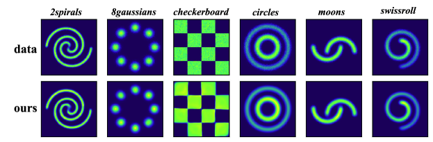
First, we focus on density estimation on synthetic data. Following the experimental setup of the previous literature (Grathwohl et al., 2020b; Liu et al., 2022b), we sample a set of 2D data points as the training set, according to some data distribution , visualized in the top of Figure 3. Then we train unnormalized models to learn this distribution, where is the multi-layer perceptrons (MLPs) with 3 hidden layers and 300 units per layer. In the experiment, We choose the SGD (or SGD-style) optimizer. For NCE, eNCE and our method, the noise distribution is selected as a multivariate Gaussian distribution, whose mean and variance are fitted on the training set.
To quantify the performance of different methods, we adopt the maximum mean discrepancy (MMD) (Gretton et al., 2012) as the criterion. The MMD metric is widely used to compare different distributions, and a lower MMD indicates that the two distributions are more similar. We sample 10000 points from the data distribution and the learned model, and the computed MMD metric is shown in Table 2. As can be seen, our method enjoys the lowest MMD among all methods for all six cases, indicating the superiority of the proposed method. Also, we report the Frechet Inception Distance (FID) score of each method, which is another widely-used measure in comparing distributions. The results are presented in Table 3, and our method enjoys better FID scores than other algorithms (smaller is better). Besides, we compare the estimated density and the ground-truth in Figure 3, showing that our method learns the density accurately in most cases. Finally, We compare different methods with the Adam optimizer and investigate the behavior of our algorithm with different values of and in the appendix.
| Dataset | AUROC↑ AUPRC↑ FRP80↓ | |
| NCE | 0.6468 ± 0.0122 0.5455 ± 0.0053 0.4929 ± 0.0301 | |
| NCE (NGD) | 0.6748 ± 0.0187 0.6265 ± 0.1565 0.5392 ± 0.0271 | |
| eNCE (NGD) | 0.7451 ± 0.0296 0.7052 ± 0.0310 0.4052 ± 0.0586 | |
| MCMC | 0.7077 ± 0.0154 0.6787 ± 0.0119 0.5137 ± 0.0253 | |
| Scoring Matching | 0.5329 ± 0.0024 0.5304 ± 0.0029 0.7706 ± 0.0047 | |
| Contrastive Divergence | 0.7735 ± 0.0161 0.7371 ± 0.0106 0.3733 ± 0.0382 | |
| CIFAR10-Interp | Ours | 0.8019 ± 0.0323 0.7679 ± 0.0402 0.3185 ± 0.0621 |
| NCE | 0.6425 ± 0.0107 0.3436 ± 0.0052 0.5592 ± 0.0286 | |
| NCE (NGD) | 0.6593 ± 0.0035 0.4361 ± 0.0083 0.7284 ± 0.0040 | |
| eNCE (NGD) | 0.6612 ± 0.0075 0.4633 ± 0.0109 0.6910 ± 0.0134 | |
| MCMC | 0.5359 ± 0.0078 0.2674 ± 0.0048 0.6327 ± 0.0037 | |
| Scoring Matching | 0.5601 ± 0.0068 0.3237 ± 0.0010 0.8346 ± 0.0060 | |
| Contrastive Divergence | 0.6103 ± 0.0040 0.3057 ± 0.0018 0.3758 ± 0.0025 | |
| SVHN | Ours | 0.7843 ± 0.0057 0.5134 ± 0.0076 0.3255 ± 0.2081 |
| NCE | 0.5323 ± 0.0199 0.5129 ± 0.0095 0.7122 ± 0.0216 | |
| NCE (NGD) | 0.5513 ± 0.0218 0.5458 ± 0.0160 0.7832 ± 0.0306 | |
| eNCE (NGD) | 0.5034 ± 0.0069 0.5248 ± 0.0158 0.8263 ± 0.0095 | |
| MCMC | 0.5669 ± 0.0059 0.5604 ± 0.0138 0.7217 ± 0.0052 | |
| Scoring Matching | 0.5732 ± 0.0014 0.5343 ± 0.0070 0.6943 ± 0.0059 | |
| Contrastive Divergence | 0.5276 ± 0.0098 0.5136 ± 0.0120 0.6642 ± 0.0111 | |
| CIFAR-100 | Ours | 0.6044 ± 0.0049 0.6262 ± 0.0079 0.5795 ± 0.0113 |
| NCE | 0.5356 ± 0.0006 0.4995 ± 0.0005 0.6876 ± 0.0028 | |
| NCE (NGD) | 0.6049 ± 0.0189 0.5817 ± 0.0083 0.7119 ± 0.0408 | |
| eNCE (NGD) | 0.5470 ± 0.0039 0.6840 ± 0.0042 0.9450 ± 0.0028 | |
| MCMC | 0.5359 ± 0.0153 0.5107 ± 0.0157 0.7436 ± 0.0131 | |
| Scoring Matching | 0.5419 ± 0.0057 0.5221 ± 0.0030 0.7372 ± 0.0097 | |
| Contrastive Divergence | 0.5044 ± 0.0054 0.4980 ± 0.0060 0.6248 ± 0.0022 | |
| LSUN-C | Ours | 0.6944 ± 0.0061 0.6267 ± 0.0046 0.5198 ± 0.0126 |
6.2 Out-of-distribution Detection
Then, we experiment on the out-of-distribution (OOD) detection, since OOD detection performance is an important measure of the density estimation quality. For this task, we choose CIFAR-10 (Krizhevsky, 2009) as the in-distribution data. We use the energy-based model as our unnormalized model, by setting , where is a 40-layer WideResNet (Zagoruyko & Komodakis, 2016). The noise distribution for NCE, eNCE and our method is selected as the multivariate Gaussian distribution, and we use Adam to optimize. For the OOD test dataset, we use four common benchmarks: CIFAR-10 Interp, SVHN (Netzer et al., 2011), CIFAR-100 (Krizhevsky, 2009), and LSUN (Yu et al., 2015). We decide whether a test sample is anomalous or not by computing the density , where a higher value indicates the test sample is more likely to be a normal sample.
To measure the performance of different methods, we follow previous works (Ren et al., 2019; Havtorn et al., 2021; Geng et al., 2021) to choose three metrics to compare: (1) area under the receiver operating characteristic curve (AUROC); (2) area under the precision-recall curve (AUPRC); and (3) false positive rate at 80% true positive rate (FPR80), where the arrow indicates the direction of improvement of the metrics. These three metrics are commonly used for evaluating OOD detection methods, and the results are reported in Table 4. As can be seen, our method performs the best under three different criteria in most cases, implying the effectiveness of the proposed method.
| NCE | NCE (NGD) | eNCE (NGD) | MCMC-OT | CF-EBM | CoopNets | Ours |
| 1.457 ± 0.003 | 1.618 ± 0.010 | 1.600 ± 0.044 | 1.441 ± 0.012 | 1.864 ± 0.004 | 1.591 ± 0.022 | 1.394 ± 0.007 |
6.3 Learning on Real Image Dataset
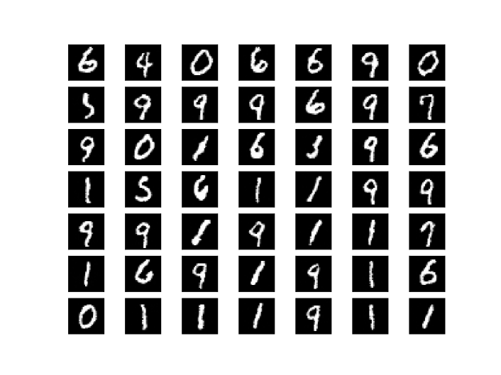
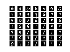
Finally, we test our method on two real image datasets, MNIST (LeCun et al., 1998) and CIFAR-10 (Krizhevsky, 2009). We describe the setup and the results of MNIST in this subsection, and results of CIFAR-10 can be found in Appendix A. For MNIST task, following the same setup in TRE (Rhodes et al., 2020), the model takes the form of , where is the 18-layer ResNet (He et al., 2016). For NCE, eNCE and our method, we try three different noise distributions: 1) the empirical distribution ; 2) multivariate Gaussian distribution, with mean and covariance fitted by the training data; 3) mixture of distribution and a multivariate Gaussian distribution. We find the last one is the best choice for all methods. We use Adam to optimize NCE, and generate new samples via MCMC sampling after training the model. The generated samples of our method with different noises are shown in the Appendix A, and the result with the third noise distribution is presented in Figure 4.
We also evaluate the learned model via estimated average negative log-likelihood (bits per dimension) on the testing sets in Table 5, which is computed by the annealed importance sampling (AIS) (Nash & Durkan, 2019). We also compare our method with some other methods, including MCMC-OT (An et al., 2021), CF-EBM (Zhao et al., 2021), and CoopNets (Xie et al., 2018). As can be seen, our method attains a better likelihood than other methods, indicating the proposed method performs better in this task.
7 Conclusion
In this paper, we investigate the problem of learning unnormalized models by maximum likelihood estimation. By introducing a noise distribution, we cast the problem as compositional optimization and utilize a stochastic algorithm to solve it. We provide the convergence rate of our method and analyze its relationship with the noise distribution. Besides, we use one-dimensional Gaussian mean estimation as an example to show the better loss landscape of our loss compared with the NCE loss, and the fast convergence of the proposed method. Finally, experiments on practical problems demonstrate the effectiveness of the proposed method.
8 Acknowledgments
W. Jiang, L. Wu and L. Zhang are partially supported by the National Key R&D Program of China (2021ZD0112802), NSFC (62122037, 61921006), and the Fundamental Research Funds for the Central Universities (2023300246).
References
- Allen-Zhu et al. (2019) Allen-Zhu, Z., Li, Y., and Song, Z. A convergence theory for deep learning via over-parameterization. In Proceedings of the 36th International Conference on Machine Learning, pp. 242–252, 2019.
- An et al. (2021) An, D., Xie, J., and Li, P. Learning deep latent variable models by short-run mcmc inference with optimal transport correction. In IEEE/CVF Conference on Computer Vision and Pattern Recognition, pp. 15410–15419, 2021.
- Bose et al. (2018) Bose, A. J., Ling, H., and Cao, Y. Adversarial contrastive estimation. In Proceedings of the 56th Annual Meeting of the Association for Computational Linguistics, pp. 1021–1032, 2018.
- Ceylan & Gutmann (2018) Ceylan, C. and Gutmann, M. U. Conditional noise-contrastive estimation of unnormalised models. In Proceedings of the 35th International Conference on Machine Learning, pp. 726–734, 2018.
- Chen et al. (2021) Chen, T., Sun, Y., and Yin, W. Solving stochastic compositional optimization is nearly as easy as solving stochastic optimization. IEEE Transactions on Signal Processing, 69:4937–4948, 2021.
- Christian P. Robert (2004) Christian P. Robert, G. C. Monte Carlo Statistical Methods. Springer, 2004.
- Cutkosky & Orabona (2019) Cutkosky, A. and Orabona, F. Momentum-based variance reduction in non-convex SGD. In Advances in Neural Information Processing Systems 32, pp. 15210–15219, 2019.
- Du et al. (2019) Du, S. S., Zhai, X., Poczos, B., and Singh, A. Gradient descent provably optimizes over-parameterized neural networks. In International Conference on Learning Representations, 2019.
- Du & Mordatch (2019) Du, Y. and Mordatch, I. Implicit generation and modeling with energy based models. In Advances in Neural Information Processing Systems 32, pp. 3603–3613, 2019.
- Fang et al. (2018) Fang, C., Li, C. J., Lin, Z., and Zhang, T. Spider: Near-optimal non-convex optimization via stochastic path integrated differential estimator. ArXiv e-prints, arXiv:1807.01695, 2018.
- Gao et al. (2018) Gao, R., Lu, Y., Zhou, J., Zhu, S.-C., and Wu, Y. N. Learning generative convnets via multi-grid modeling and sampling. In Proceedings of the IEEE/CVF Conference on Computer Vision and Pattern Recognition, pp. 9155–9164, 2018.
- Geng et al. (2021) Geng, C., Wang, J., Gao, Z., Frellsen, J., and Hauberg, S. Bounds all around: training energy-based models with bidirectional bounds. In Advances in Neural Information Processing Systems 34, pp. 19808–19821, 2021.
- Ghadimi et al. (2020) Ghadimi, S., Ruszczynski, A., and Wang, M. A single timescale stochastic approximation method for nested stochastic optimization. SIAM Journal on Optimization, 30(1):960–979, 2020.
- Goodfellow et al. (2014) Goodfellow, I., Pouget-Abadie, J., Mirza, M., Xu, B., Warde-Farley, D., Ozair, S., Courville, A., and Bengio, Y. Generative adversarial nets. In Advances in Neural Information Processing Systems 27, pp. 2672–2680, 2014.
- Grathwohl (2020) Grathwohl, W. Joint energy models. https://github.com/wgrathwohl/JEM, 2020.
- Grathwohl et al. (2020a) Grathwohl, W., Wang, K.-C., Jacobsen, J.-H., Duvenaud, D., Norouzi, M., and Swersky, K. Your classifier is secretly an energy based model and you should treat it like one. In International Conference on Learning Representations, 2020a.
- Grathwohl et al. (2020b) Grathwohl, W., Wang, K.-C., Jacobsen, J.-H., Duvenaud, D., and Zemel, R. Learning the stein discrepancy for training and evaluating energy-based models without sampling. In Proceedings of the 37th International Conference on Machine Learning, pp. 3732–3747, 2020b.
- Gretton et al. (2012) Gretton, A., Borgwardt, K. M., Rasch, M. J., Schölkopf, B., and Smola, A. A kernel two-sample test. Journal of Machine Learning Research, 13(25):723–773, 2012.
- Guo et al. (2021) Guo, Z., Xu, Y., Yin, W., Jin, R., and Yang, T. On stochastic moving-average estimators for non-convex optimization. ArXiv e-prints, arXiv:2104.14840, 2021.
- Gutmann & Hyvärinen (2010) Gutmann, M. U. and Hyvärinen, A. Noise-contrastive estimation: A new estimation principle for unnormalized statistical models. In Proceedings of the 13th International Conference on Artificial Intelligence and Statistics, pp. 297–304, 2010.
- Gutmann & Hyvärinen (2012) Gutmann, M. U. and Hyvärinen, A. Noise-contrastive estimation of unnormalized statistical models, with applications to natural image statistics. Journal of Machine Learning Research, 13(11):307–361, 2012.
- Han et al. (2019) Han, T., Nijkamp, E., Fang, X., Hill, M., Zhu, S., and Wu, Y. N. Divergence triangle for joint training of generator model, energy-based model, and inferential model. In Proceedings of the IEEE/CVF Conference on Computer Vision and Pattern Recognition, pp. 8670–8679, 2019.
- Havtorn et al. (2021) Havtorn, J. D., Frellsen, J., Hauberg, S., and Maaløe, L. Hierarchical VAEs know what they don’t know. In Proceedings of the 38th International Conference on Machine Learning, pp. 4117–4128, 2021.
- He et al. (2016) He, K., Zhang, X., Ren, S., and Sun, J. Deep residual learning for image recognition. In Proceedings of the IEEE/CVF Conference on Computer Vision and Pattern Recognition, pp. 770–778, 2016.
- Henaff (2020) Henaff, O. Data-efficient image recognition with contrastive predictive coding. In Proceedings of the 37th International Conference on Machine Learning, pp. 4182–4192, 2020.
- Hinton (2002) Hinton, G. E. Training products of experts by minimizing contrastive divergence. Neural computation, 14(8):1771–1800, 2002.
- Hjelm et al. (2019) Hjelm, R. D., Fedorov, A., Lavoie-Marchildon, S., Grewal, K., Bachman, P., Trischler, A., and Bengio, Y. Learning deep representations by mutual information estimation and maximization. In International Conference on Learning Representations, 2019.
- Hyvärinen (2005) Hyvärinen, A. Estimation of non-normalized statistical models by score matching. Journal of Machine Learning Research, 6(24):695–709, 2005.
- Jiang et al. (2022a) Jiang, W., Li, G., Wang, Y., Zhang, L., and Yang, T. Multi-block-single-probe variance reduced estimator for coupled compositional optimization. In Advances in Neural Information Processing Systems 35, 2022a.
- Jiang et al. (2022b) Jiang, W., Wang, B., Wang, Y., Zhang, L., and Yang, T. Optimal algorithms for stochastic multi-level compositional optimization. In Proceedings of the 39th International Conference on Machine Learning, pp. 10195–10216, 2022b.
- Jianwen et al. (2018) Jianwen, X., Lu, Y., Zhu, S., and Wu, Y. Cooperative training of descriptor and generator networks. IEEE transactions on pattern analysis and machine intelligence, 2018.
- Karimi et al. (2016) Karimi, H., Nutini, J., and Schmidt, M. Linear convergence of gradient and proximal-gradient methods under the Polyak-Łojasiewicz condition. In Machine Learning and Knowledge Discovery in Databases, pp. 795–811, 2016.
- Kong et al. (2020) Kong, L., de Masson d’Autume, C., Yu, L., Ling, W., Dai, Z., and Yogatama, D. A mutual information maximization perspective of language representation learning. In International Conference on Learning Representations, 2020.
- Krizhevsky (2009) Krizhevsky, A. Learning multiple layers of features from tiny images. Masters Thesis, Deptartment of Computer Science, University of Toronto, 2009.
- LeCun et al. (1998) LeCun, Y., Bottou, L., Bengio, Y., and Haffner, P. Gradient-based learning applied to document recognition. In Proceedings of the IEEE, pp. 2278–2324, 1998.
- LeCun et al. (2006) LeCun, Y., Chopra, S., Hadsell, R., Ranzato, A., and Huang, F. J. A tutorial on energy-based learning. Predicting structured data, 2006.
- Liu et al. (2022a) Liu, B., Rosenfeld, E., Ravikumar, P. K., and Risteski, A. Analyzing and improving the optimization landscape of noise-contrastive estimation. In International Conference on Learning Representations, 2022a.
- Liu et al. (2022b) Liu, M., Liu, H., and Ji, S. Gradient-guided importance sampling for learning binary energy-based models. ArXiv e-prints, arXiv:2210.05782, 2022b.
- Mnih & Kavukcuoglu (2013) Mnih, A. and Kavukcuoglu, K. Learning word embeddings efficiently with noise-contrastive estimation. In Advances in Neural Information Processing Systems 26, pp. 2265–2273, 2013.
- Nash & Durkan (2019) Nash, C. and Durkan, C. Autoregressive energy machines. In Proceedings of the 36th International Conference on Machine Learning, pp. 1735–1744, 2019.
- Netzer et al. (2011) Netzer, Y., Wang, T., Coates, A., Bissacco, A., Wu, B., and Ng, A. Y. Reading digits in natural images with unsupervised feature learning. In Advances in Neural Information Processing Systems Workshop on Deep Learning and Unsupervised Feature Learning, 2011.
- Nguyen et al. (2017) Nguyen, L. M., Liu, J., Scheinberg, K., and Takac, M. SARAH: A novel method for machine learning problems using stochastic recursive gradient. In Proceedings of the 34th International Conference on Machine Learning, pp. 2613–2621, 2017.
- Nijkamp et al. (2019a) Nijkamp, E., Hill, M., Han, T., Zhu, S.-C., and Wu, Y. N. On the anatomy of MCMC-based maximum likelihood learning of energy-based models. In Proceedings of the 33th AAAI Conference on Artificial Intelligence, 2019a.
- Nijkamp et al. (2019b) Nijkamp, E., Hill, M., Zhu, S.-C., and Wu, Y. N. Learning non-convergent non-persistent short-run MCMC toward energy-based model. In Advances in Neural Information Processing Systems 32, pp. 5233–5243, 2019b.
- Pang et al. (2020) Pang, T., Xu, K., LI, C., Song, Y., Ermon, S., and Zhu, J. Efficient learning of generative models via finite-difference score matching. In Advances in Neural Information Processing Systems 33, pp. 19175–19188, 2020.
- Qi et al. (2021a) Qi, Q., Guo, Z., Xu, Y., Jin, R., and Yang, T. An online method for a class of distributionally robust optimization with non-convex objectives. ArXiv e-prints, arXiv:2006.10138, 2021a.
- Qi et al. (2021b) Qi, Q., Luo, Y., Xu, Z., Ji, S., and Yang, T. Stochastic optimization of areas under precision-recall curves with provable convergence. In Advances in Neural Information Processing Systems 34, pp. 1752–1765, 2021b.
- Ren et al. (2019) Ren, J., Liu, P. J., Fertig, E., Snoek, J., Poplin, R., Depristo, M., Dillon, J., and Lakshminarayanan, B. Likelihood ratios for out-of-distribution detection. In Advances in Neural Information Processing Systems 32, pp. 14680–14691, 2019.
- Rhodes et al. (2020) Rhodes, B., Xu, K., and Gutmann, M. U. Telescoping density-ratio estimation. In Advances in Neural Information Processing Systems 33, pp. 4905–4916, 2020.
- Ruiqi et al. (2020) Ruiqi, G., Nijkamp, E., Kingma, D., Xu, Z., Dai, A., and Wu, Y. Flow contrastive estimation of energy-based models. In Proceedings of the IEEE/CVF Conference on Computer Vision and Pattern Recognition, pp. 7518–7528, 2020.
- Seitzer (2020) Seitzer, M. pytorch-fid: FID Score for PyTorch, 2020.
- Song & Ermon (2019) Song, Y. and Ermon, S. Generative modeling by estimating gradients of the data distribution. In Advances in Neural Information Processing Systems 32, pp. 11895–11907, 2019.
- Song et al. (2019) Song, Y., Garg, S., Shi, J., and Ermon, S. Sliced score matching: A scalable approach to density and score estimation. In Proceedings of the 35th Conference on Uncertainty in Artificial Intelligence, 2019.
- Tian et al. (2020) Tian, Y., Krishnan, D., and Isola, P. Contrastive Multiview Coding. Springer, 2020.
- Tieleman (2008) Tieleman, T. Training restricted Boltzmann machines using approximations to the likelihood gradient. In Proceedings of the 25th International Conference on Machine Learning, 2008.
- Vaart (1998) Vaart, A. W. v. d. Asymptotic Statistics. Cambridge University Press, 1998.
- Vincent (2011) Vincent, P. A connection between score matching and denoising autoencoders. Neural Computation, 23(7):1661–1674, 2011.
- Wang & Yang (2022) Wang, B. and Yang, T. Finite-sum coupled compositional stochastic optimization: Theory and applications. In Proceedings of the 39th International Conference on Machine Learning, pp. 23292–23317, 2022.
- Wang et al. (2016) Wang, M., Liu, J., and Fang, E. Accelerating stochastic composition optimization. In Advances in Neural Information Processing Systems 29, pp. 1714–1722, 2016.
- Wang et al. (2017a) Wang, M., Fang, E. X., and Liu, H. Stochastic compositional gradient descent: algorithms for minimizing compositions of expected-value functions. Mathematical Programming, 161(1-2):419–449, 2017a.
- Wang et al. (2017b) Wang, M., Liu, J., and Fang, E. X. Accelerating stochastic composition optimization. Journal of Machine Learning Research, 18:105:1–105:23, 2017b.
- Wasserman (2004) Wasserman, L. All of Statistics. Springer, 2004.
- Welling & Teh (2011) Welling, M. and Teh, Y. W. Bayesian learning via stochastic gradient langevin dynamics. In Proceedings of the 28th International Conference on Machine Learning, 2011.
- Xie et al. (2016) Xie, J., Lu, Y., Zhu, S.-C., and Wu, Y. N. A theory of generative convnet. In Proceedings of the 33rd International Conference on International Conference on Machine Learning, pp. 2635–2644, 2016.
- Xie et al. (2018) Xie, J., Lu, Y., Gao, R., and Wu, Y. N. Cooperative learning of energy-based model and latent variable model via mcmc teaching. In Proceedings of the AAAI Conference on Artificial Intelligence, 2018.
- Xie et al. (2021) Xie, J., Zheng, Z., and Li, P. Learning energy-based model with variational auto-encoder as amortized sampler. In Proceedings of the AAAI Conference on Artificial Intelligence, 2021.
- Xie et al. (2022) Xie, J., Zhu, Y., Li, J., and Li, P. A tale of two flows: Cooperative learning of langevin flow and normalizing flow toward energy-based model. In International Conference on Learning Representations, 2022.
- Yu et al. (2015) Yu, F., Seff, A., Zhang, Y., Song, S., Funkhouser, T., and Xiao, J. LSUN: Construction of a large-scale image dataset using deep learning with humans in the loop. ArXiv e-prints, arXiv:1506.03365, 2015.
- Yu et al. (2020) Yu, L., Song, Y., Song, J., and Ermon, S. Training deep energy-based models with f-divergence minimization. In Proceedings of the 37th International Conference on Machine Learning, volume 119, pp. 10957–10967, 2020.
- Zagoruyko & Komodakis (2016) Zagoruyko, S. and Komodakis, N. Wide residual networks. In Proceedings of the British Machine Vision Conference, 2016.
- Zhang & Xiao (2019) Zhang, J. and Xiao, L. A stochastic composite gradient method with incremental variance reduction. In Advances in Neural Information Processing Systems 32, pp. 9075–9085, 2019.
- Zhang & Xiao (2021) Zhang, J. and Xiao, L. Multilevel composite stochastic optimization via nested variance reduction. SIAM Journal on Optimization, 31(2):1131–1157, 2021.
- Zhao et al. (2021) Zhao, Y., Xie, J., and Li, P. Learning energy-based generative models via coarse-to-fine expanding and sampling. In International Conference on Learning Representations, 2021.
Appendix A Omitted Experimental Results
In this section, we present omitted experimental results on the task of density estimation and image generation.
A.1 More Results on Density Estimation
Results for Adam optimizer
First, we show the performance of different methods with Adam (or Adam-style) optimizer in the task of Density Estimation on Synthetic Data. The results are shown in Table 6 and Table 7. As can be seen, our method performs better than other algorithms in most cases.
| Method | 2spirals | 8gaussians | checkerboard | circles | moons | swissroll |
| NCE | 3.230 ± 0.460 | 0.130 ± 0.055 | 1.710 ± 0.190 | 1.045 ± 0.208 | 4.588 ± 0.688 | 1.510 ± 0.498 |
| NCE (NGD) | 2.533 ± 0.716 | 0.128 ± 0.020 | 1.807 ± 0.451 | 0.947 ± 0.265 | 4.202 ± 0.474 | 1.576 ± 0.589 |
| eNCE (NGD) | 2.585 ± 0.841 | 0.146 ± 0.082 | 1.690 ± 0.264 | 0.968 ± 0.342 | 3.852 ± 0.957 | 1.604 ± 0.490 |
| MCMC | 2.342 ± 0.658 | 0.178 ± 0.105 | 1.710 ± 0.394 | 0.937 ± 0.387 | 3.680 ± 0.916 | 1.438 ± 0.375 |
| Score Matching | 2.727 ± 0.579 | 0.135 ± 0.071 | 3.130 ± 0.497 | 1.706 ± 0.309 | 5.296 ± 0.221 | 2.874 ± 0.688 |
| Contrastive Divergence | 2.516 ± 0.984 | 0.173 ± 0.066 | 1.683 ± 0.904 | 0.927 ± 0.432 | 3.904 ± 0.914 | 1.498 ± 0.368 |
| Ours | 2.488 ± 0.356 | 0.117 ± 0.086 | 1.651 ± 0.166 | 0.886 ± 0.129 | 3.644 ± 0.490 | 1.338 ± 0.131 |
| Method | 2spirals | 8gaussians | checkerboard | circles | moons | swissroll |
| NCE | 0.053 ± 0.030 | 0.096 ± 0.042 | 0.156 ± 0.121 | 0.068 ± 0.028 | 0.046 ± 0.031 | 0.159 ± 0.069 |
| NCE (NGD) | 0.067 ± 0.315 | 0.104 ± 0.038 | 0.167 ± 0.091 | 0.061 ± 0.030 | 0.029 ± 0.017 | 0.171 ± 0.065 |
| eNCE (NGD) | 0.072 ± 0.053 | 0.127 ± 0.085 | 0.102 ± 0.081 | 0.066 ± 0.046 | 0.038 ± 0.032 | 0.205 ± 0.035 |
| MCMC | 0.047 ± 0.025 | 0.107 ± 0.073 | 0.097 ± 0.084 | 0.049 ± 0.028 | 0.052 ± 0.021 | 0.161 ± 0.088 |
| Score Matching | 0.070 ± 0.024 | 0.087 ± 0.050 | 0.231 ± 0.110 | 0.086 ± 0.034 | 0.037 ± 0.018 | 0.190 ± 0.148 |
| Contrastive Divergence | 0.064 ± 0.025 | 0.092 ± 0.034 | 0.093 ± 0.034 | 0.076 ± 0.038 | 0.062 ± 0.022 | 0.148 ± 0.029 |
| Ours | 0.040 ± 0.026 | 0.067 ± 0.030 | 0.086 ± 0.101 | 0.040 ± 0.035 | 0.028 ± 0.037 | 0.144 ± 0.078 |
Results with different and
Then, we investigate the behavior of our algorithm with different values of and . In the previous experiment, we simply set and . Here, we first fix and enumerate from the set . Then, we fix and enumerate from the set . The results are reported in Table 8 and Table 9, which indicates that our method is not very sensitive to the choice of and within a certain range.
| value | 2spirals | 8gaussians | checkerboard | circles | moons | swissroll |
| 3.355 ± 0.781 | 0.168 ± 0.098 | 1.889 ± 0.506 | 1.355 ± 0.164 | 4.762 ± 0.192 | 2.784 ± 0.618 | |
| 3.040 ± 0.199 | 0.132 ± 0.098 | 1.645 ± 0.251 | 1.075 ± 0.169 | 4.673 ± 0.519 | 2.566 ± 0.274 | |
| 3.038 ± 0.395 | 0.150 ± 0.078 | 1.603 ± 0.258 | 1.120 ± 0.211 | 4.816 ± 0.292 | 2.528 ± 0.371 |
| Method | 2spirals | 8gaussians | checkerboard | circles | moons | swissroll |
| 2.982 ± 0.304 | 0.141 ± 0.106 | 1.730 ± 0.716 | 1.345 ± 0.198 | 4.650 ± 0.302 | 2.595 ± 0.493 | |
| 3.040 ± 0.199 | 0.132 ± 0.098 | 1.645 ± 0.251 | 1.075 ± 0.169 | 4.673 ± 0.519 | 2.566 ± 0.274 | |
| 3.168 ± 0.360 | 0.145 ± 0.052 | 1.718 ± 0.418 | 1.152 ± 0.109 | 4.772 ± 0.651 | 2.648 ± 0.601 |
A.2 More Results on Image Generation
Training EBM on MNIST
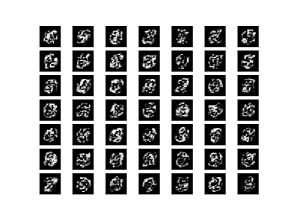
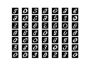
To verify our analysis for the noise distribution, we compare the image generation results with different noises: 1) the empirical distribution ; 2) Gaussian distribution with its mean and variance fitted on the training data; 3) mixture of empirical distribution and a fitted Gaussian noise. The results are shown in Figure 5. As can be seen, the first two cases perform poorly and only the third case generates images similar to the original MNIST dataset, which is consistent with our suggestions.
Training EBM on CIFAR-10
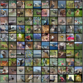
We further test our method on the more complex CIFAR-10 dataset. We use the codebase of the JEM model (Grathwohl et al., 2020a), which performs generation and classification simultaneously. We replace the standard EBM with Langevin dynamics with our proposed method, and follow exactly the same parameter setting as specified in the codebase (Grathwohl, 2020). We test our method for both classification and image generation tasks, and compare with the original JEM method. For this sets of experiments on more complex natural images, we find that it is more important to design an appropriate noise distribution. Our empirical distribution + noise method does not work well in this case, partially due to the fact that the empirical data are too sparsely located at the complex data manifold. Consequently, the estimated density can induce too large variance, leading to slow convergence. We mitigate the limitation by introducing a few MCMC steps (around 10) by directly starting from a pool of updating negative samples, and adopt the kernel density estimation to approximate the density values (as they do not have closed forms after MCMC steps). We find this is essential for learning to generate high-quality real images. Note our adopted method still has limitations, for example, it still requires MCMC steps that we want to avoid, and the estimated densities are not accurate enough. We thus leave designing a good noise estimation for more advanced image generation as interesting future work. Following the instruction in the codebase, we achieve a classification accuracy of 90.72% with a loss of 0.34, compared to an accuracy of 89.38% and a loss of 0.39 from the JEM. Regarding the generated image quality, we measure it with the Inception Score (IS) and Fréchet Inception Distance (FID) score (Seitzer, 2020), based on 10k generated images. Our method obtains an improved FID score from 54.76 to 51.77, while maintaining comparable IS scores, i.e., 4.79 (ours) versus 4.83 (JEM). Note that these numbers are a little worse than what were reported in the JEM paper, mostly due to different experimental settings111As confessed by the JEM author, their reported results need heavily manual tuning, which is not easily reproduced (see issue #7 in the codebase). The results are also far from the current state-of-the-arts. However, our goal is only to demonstrate the effectiveness of our method compared to the standard EBM training under a simple setting. Thus, our results are reasonable and the comparison is fair. . Some generated samples from our method are plotted in Figure 6.
Appendix B Analysis
In this section, we present the proof of all theorems.
B.1 Proof of Theorem 1
Here, we prove the first property of Theorem 1. The other properties — asymptotically normal and asymptotically optimal can be obtained according to the property of MLE (for example, see Chapter 9 in Wasserman (2004)).
We note that the minimizing of is equivalent to minimizing
By the law of large numbers, as the sample size increases, converges to
where means the Kullback-Leibler distance between and . Hence, we have .
Then, we prove the first property — consistent is satisfied under the following conditions.
Since minimizes , we have and
It follows that, for any ,
Select any . By condition 2), there exists such that implies that . Hence,
B.2 Proof of Theorem 2
First, we prove the following supporting lemmas. We simplify the notation as and as .
Lemma 2.
We show that the estimation errors of and would be reduced over time.
Proof.
Consider the update , , and set .
where the last inequality is due to the fact that .
According to Assumption 1, we know that is also -Lipchitz continuous and -smooth, where and . By setting , we have:
∎
To finish the proof, we also need to introduce the following lemma.
Lemma 3.
(Guo et al., 2021) Suppose function is -smooth and consider the update . With , we have:
According to above lemmas, we have:
Summing up, we have:
where
By setting and , where and , we have:
According to the analysis of previous works, such as NASA (Ghadimi et al., 2020), since a.s., and , we would have , , , otherwise the left part of above equation tends to infinity, while the right part is not.
B.3 Proof of Theorem 3
With supporting lemmas in previous theorem, by setting , we have:
where .
Similarly, for the term , we have:
So, we have
where , , is the constant.
Define the . We can have:
To hide the constant, we finally have . We can easily extend the results to the case of adaptive learning rates in the style of Adam, following the analysis of Guo et al. (2021).
B.4 Proof of Theorem 4
If is -PL, which is , we can further improve the rate.
Define that , and then we have:
Setting , we have:
Define , we have:
If , set , which is .
We have , so we have , where Finally, we have .
So . The complexity is .
If , set , and the complexity is .
B.5 Proof of Lemma 1
We analyze the variance of our estimator . By setting , the variance of our estimator is
To get the minimum variance, we should choose and the variance would be zero.
B.6 Proof of Proposition 2
First, we write the MLE objective function as:
So, we have:
B.7 Proof of Proposition 3
We prove that the objective is -strongly convex, which is a stronger condition than -PL condition.
Assume that and we have:
The last equation is due to the fact that the variance is fixed as 1 for the model. So, the objective is -strongly convex, and according to our analysis for PL condition, our method enjoys a complexity of due to Theorem 4.