Holographic RG from ERG: Locality and General Coordinate Invariance in the Bulk

Abstract

In earlier papers it was shown that the correct kinetic term for scalar, vector gauge field and the spin two field in $AdS_{D+1}$ space is obtained starting from the ERG equation for a $CFT_{D}$ perturbed by scalar composite, conserved vector current and conserved traceless energy momentum tensor respectively. In this paper interactions are studied and it is shown that a flipped version of Polchinski ERG equation that evolves towards the UV can be written down and is useful for making contact with the usual AdS/CFT prescriptions for correlation function calculations. The scalar-scalar-spin-2 interaction in the bulk is derived from the ERG equation in the large $N$ semiclasical approximation. It is also shown that after mapping to AdS the interaction is local on a scale of the bare cutoff rather than the moving cutoff (which would have corresponded to the AdS scale). The map to $AdS_{D+1}$ plays a crucial role in this locality. The local nature of the coupling ensures that this interaction term in the bulk action is obtained by gauge fixing a general coordinate invariant scalar kinetic term in the bulk action. A wave function renormalization of the scalar field is found to be required for a mutually consistent map of the two fields to $AdS_{D+1}$.

1 Introduction

A precise realization of the holographic idea [1, 2] is the AdS/CFT correspondence [[3]-[7]]. One of the most interesting ideas that have come out of the AdS/CFT correspondence is that of Holographic RG [[8]-[22]]. It has been shown in a series of papers [24, 25, 26, 27] that in some cases Holographic RG can be derived from first principles starting from a Polchinski ERG equation [[28]-[37]] of the boundary CFT . The particular duality considered in those works is the conjectured duality [39] between free $O(N)$ vector model in $D=3$ and Vasiliev higher spin theory in $D=4$ [42]. The evolution operator for Polchinski’s ERG equation of the $D$-dimensional field theory can be written as a functional integral of the $D+1$ dimensional field theory. This is already holographic, but this field theory has a non standard (and non local) kinetic term. In [24] it was shown that a special field redefinition maps this to a local kinetic term in $AdS_{D+1}$. The holographic bulk action being an evolution operator for an ERG equation, both before the map to $AdS_{D+1}$ and after, is guaranteed to reproduce correlation functions of the boundary theory. In fact any (non singular) field redefinition can be done without spoiling this property. In [38] other maps were explored and some were shown to have interesting properties. What is nice about the map to $AdS_{D+1}$ is that the kinetic term for the scalar field is local. This was extended in [26] to composite operators of the boundary theory. In [27] this was done for conerved vector currents and conserved energy momentum tensor. In the first case one obtains a kinetic term for a gauge fixed gauge field in the bulk. In the second case one obtains a kinetic term for a metric perturbation about an AdS background in a special gauge. Thus one obtains dynamical gauge fields and gravity starting from ERG of a boundary CFT. This is remarkable. In all this it is important to note that the validity of the AdS-CFT conjecture is not assumed. The bulk theory is guaranteed to reproduce correlations of the boundary theory because it is just implementing RG evolution. All this is clearly related to the problem often referred to as “bulk reconstruction”.

Exact Renormalization Group has earlier been interpreted as the essence behind AdS/CFT in [43, 44, 45, 46].

The form of the AdS metric makes it natural for the moving cutoff in the ERG to be mapped to the radial coordinate. The special role played by AdS space so far in this approach is that the kinetic term of the bulk scalar, which was non local to begin with, becomes local when mapped to AdS space.

The natural question that can be asked is whether this property persists for the interaction terms in the bulk. This was partially addressed in [26]. The cubic scalar coupling in the bulk was derived starting from the ERG equation. It was shown to reproduce the correlation function of the boundary theory (as expected). The locality issue was addressed and it was shown that with some assumptions the interaction can be made local.

A conceptual issue in relating Wilsonian ERG to AdS/CFT is that the AdS/CFT prescription involves integration of the bulk moving outwards to large radius—towards the UV [16]. Wilsonian RG naturally starts with a UV region and moves inward. We show in this paper that a flipped ERG equation that evolves to the UV can easily be written down simply by interchanging the low and high energy propagators. They lead to the same results. This equation is unnatural physically from the point of view of RG, but is mathematically valid and corresponds more naturally to the usual AdS/CFT holographic RG calculations. In holographic RG one places the boundary at $z=\epsilon$ and imposes boundary conditions on this surface and, (in pure AdS which is what we consider in this paper), at $z=\infty$ one requires the fields to vanish. $\epsilon$ is taken to zero at the end. In the field theory this corresponds to taking the UV cutoff $\Lambda\to\infty$. We evaluate the cubic interaction using the flipped UV version of the ERG equation. While we have incorporated the cutoff $\epsilon$ in the calculations for obtaining the expressions, these must be renormalised as prescribed in [23] to get finite expressions.

In this paper we also address this issue of locality more carefully. In the (semiclassical) bulk calulation of the boundary correlation function one finds that the final result for the correlation function is independent of the details of dependence of the Green function on the moving cutoff. This is true for any field redefinition. However for the particular field redefinition that gives AdS space it turns out that this freedom can be fruitfully used to make the interaction vertex local. This is intimately tied to the conformal nature of the correlation functions. In particular we calculate the cubic scalar-scalar-spin 2 coupling and find that it can be made local in this manner. Thus, just as with the kinetic term, the map that gives AdS space is picked out as special by the requirement of locality of the cubic coupling as well. Locality requires incorporating the correct falloff conditions for the bulk fields, i.e., the leading term in powers of $z$ for the scalar should be the boundary operator vev and the for the graviton it should be the source for the operator.

The locality of the coupling of the massless spin 2 field has implications for general coordinate invariance of the theory. If one starts with a general coordinate invariant scalar kinetic term and expands about an AdS background, the linear coupling of the metric perturbation in an appropriate gauge reduces to precisely this local coupling. Hence one can conclude that this term is consistent with general coordinate invariance of the theory [47, 48, 49, 50, 51]. It also implies that if one performs a coordinate transformation, the modification of the AdS background metric can be absorbed by the dynamical graviton as a gauge transformation—equivalently it changes the fixed gauge to some other gauge.

One of the technical issues one faces in calculating the graviton-scalar-scalar coupling is that of consistently mapping the kinetic terms of both the composite scalar and spin 2 composite energy momentum tensor (which becomes a graviton in the bulk) to the correct AdS form. As was pointed out in [27], since both kinetic terms are made up of the fundamental scalar kinetic term with a specific cutoff function, it is not possible to map them both simultaneously. The way out of this problem is to perform an additional wave function renormalization of the composite scalar field. This gives some freedom to modify the cutoff dependence of the composite scalar kinetic term at high energies. It becomes possible then to map both kinetic terms to the AdS form simultaneously.

All these issues have also to be generalized to higher spins. The RG approach for higher spins was discussed in [46] and these ideas were further developed in [52, 53]. It would be interesting to apply the ideas of the present paper to these situations also and understand the higher symmetries discussed there.

This paper is organized as follows: In Section 3, we discuss the general coordinate invariance of the theory and the issue of gauge (coordinate) transformations. In Section 4, the flipped ERG equation is worked out and the connection with the usual formulations of the AdS/CFT correspondence is explained. In Section 5 the locality of the cubic scalar coupling is explained. The map to AdS space is also given and it is shown that it leads to a local interaction term in the bulk. Section 6 discusses this issue for the graviton-scalar-scalar coupling, and section 7 has the mapping of this term to AdS. Section 8 contains a summary, conclusions and some open questions. The appendices contain supplementary calculations, viz., the mapping to AdS for the tensor in A, the issue of consistency of simultaneously mapping the scalar and the tensor by our procedure in B, and the computation of the scalar-scalar-tensor vertex integral in C.

2 A Note on Notation

In several places below we omit the measure in integrals to make the equations more readable. Instead we indicate the parameter to be integrated over with a subscript, like so: $\int_{x}$. More specifically, when a momentum is being integrated over,

$$\int_{p}\equiv\int\frac{\mathrm{d}p^{D}}{(2\pi)^{D}},$$ (2.1)

where $D$ is the number of dimensions of the boundary manifold.

3 General Coordinate Invariance

3.1 Gauge fixing a General Coordinate Invariant Action

3.1.1 Free Theory

In [27] it was shown that starting from the ERG equation for a free O(N) scalar field theory perturbed by the term $h^{\mu\nu}T_{\mu\nu}$, (where $T_{\mu\nu}$ is the improved energy momentum tensor), in the boundary of AdS, one can construct a bulk dual action for a free massless spin 2 field in the AdS bulk. In the boundary theory this spin 2 tensor is an auxiliary field standing for the traceless conserved energy momentum tensor composite field. In the bulk a massless spin 2 field must be a graviton. This is confirmed by comparing this action with a bulk calculation. To be more precise, one starts with the Einstein action and takes the metric in the form $(g_{AdS})_{MN}+h_{MN}$, where $(g_{AdS})_{MN}$ ($M=1,...,D+1$ )is the background $AdS_{D+1}$ metric given by

$$ds^{2}=\frac{dz^{2}+\delta_{\mu\nu}dx^{\mu}dx^{\nu}}{z^{2}}.$$

and $h_{MN}$ is a small deviation. Extract the quadratic action for $h_{MN}$ from the Einstein action. One can set ($x^{M}=(z,x^{\mu})$) (in the gauge $h_{zM}=0$)

$$h_{zz}=0=h_{\mu z}=\partial^{\mu}h_{\mu\nu}=h^{\mu}_{\mu}.$$ (3.1)

This is a transverse-traceless gauge. The quadratic action so obtained, i.e. by gauge fixing a general coordinate invariant action is [47, 48, 49, 50]

$$S=\frac{1}{2}\int dz\frac{d^{D}p}{(2\pi)^{D}}~{}z^{1-D}[z^{4}\partial_{z}h_{\mu\nu}\partial^{z}h^{\mu\nu}+\partial_{\rho}h_{\mu\nu}\partial^{\rho}h^{\mu\nu}+4z^{3}h_{\mu\nu}\partial_{z}h^{\mu\nu}+4z^{2}h_{\mu\nu}h^{\mu\nu}].$$ (3.2)

Indices are raised in the above action using $\delta^{MN}$. Setting $h_{\mu\nu}z^{2}=y_{\mu\nu}$,

$$S=\frac{1}{2}\int d^{D+1}x~{}z^{-D+1}~{}[\partial_{z}y_{\mu\nu}\partial^{z}y^{\mu\nu}+\partial_{\rho}y_{\mu\nu}\partial^{\rho}y^{\mu\nu}].$$ (3.3)

This is compared with what is obtained from ERG and one finds that there is agreement [27]. Thus one can say that at the free level, a dynamical gravity consistent with general coordinate invariance is obtained starting from the ERG equation of a boundary CFT in flat space. That dynamical gravity emerges from ERG is conceptually remarkable.

3.1.2 Interactions

One can further test general coordinate invariance at the interacting level as follows. The ERG procedure applied to a scalar composite of the boundary theory generates an action [26]

$$S=\frac{1}{2}\int_{x}\sqrt{g_{AdS}}~{}g_{AdS}^{MN}\partial_{M}\phi\partial_{N}\phi.$$ (3.4)

Here $\int_{x}\equiv\int\mathrm{d}x^{D+1}$.

Let us analyse this from the bulk viewpoint. Our bulk starting point is a general coordinate invariant action:

$$S=\frac{1}{2}\int_{x}\sqrt{g}~{}g^{MN}\partial_{M}\phi\partial_{N}\phi.$$ (3.5)

If we expand about $AdS$ background $g_{MN}=(g_{AdS})_{MN}+h_{MN}$ one expects a graviton-scalar-scalar coupling of the form

$$S=\frac{1}{2}\int_{x}\sqrt{g_{AdS}}~{}[g_{AdS}^{MN}\partial_{M}\phi\partial_{N}\phi+~{}h^{MN}\partial_{M}\phi\partial_{N}\phi].$$ (3.6)

(The $\sqrt{g}$ does not contribute a term linear in $h$ if it is traceless.) In the gauge (3.1) the interaction term becomes

$$S=\frac{1}{2}\int_{x}\sqrt{g_{AdS}}~{}h^{\mu\nu}\partial_{\mu}\phi\partial_{\nu}\phi.$$ (3.7)

In this paper we will verify that such a coupling does indeed exist. This shows that the action obtained from ERG is general coordinate invariant to this order.

Since the action obtained in the bulk using the ERG procedure can be obtained by gauge fixing a general coordinate invariant theory, one concludes that the bulk theory obtained by the ERG procedure is indeed a general coordinate invariant theory of gravity. One can then ask whether it is possible to change gauge from (3.1) to some other gauge. This should be equivalent to a coordinate transformation. Thus we are interested in studying the change in form due to a coordinate transformation (change of variables).

We start with

$$S=\frac{1}{2}\int_{x}\sqrt{G}~{}G^{MN}\partial_{M}\phi\partial_{N}\phi.$$

Here $G_{MN}$ has the functional form of an $AdS$ metric but is not a dynamical field. Thus to begin with $G_{MN}=(g_{AdS})_{MN}$. Under a change of coordinates

$$G^{MN}(x)=G^{MN}(x^{\prime}+\epsilon(x^{\prime}))=G^{MN}(x^{\prime})+\epsilon^{P}(x^{\prime})\partial_{P}G^{MN}(x^{\prime}),$$

$$\frac{\partial\phi(x)}{\partial x^{M}}=\bigg{(}\delta^{Q}_{M}-\frac{\partial\epsilon^{Q}}{\partial x^{M}}\bigg{)}\frac{\partial\phi(x^{\prime}+\epsilon)}{\partial x^{\prime Q}},$$

$$\sqrt{G}G^{MN}(x)\partial_{M}\phi(x)\partial_{N}\phi(x)=\sqrt{G}G^{MN}\frac{\partial\phi(x^{\prime})}{\partial x^{\prime M}}\frac{\partial\phi(x^{\prime})}{\partial x^{\prime N}}+\epsilon^{R}\partial_{R}\bigg{(}\sqrt{G}G^{MN}\frac{\partial\phi(x^{\prime})}{\partial x^{\prime M}}\frac{\partial\phi(x^{\prime})}{\partial x^{\prime N}}\bigg{)}$$

$$-\sqrt{G}\bigg{(}\frac{\partial\epsilon^{M}}{\partial x^{Q}}G^{QN}+\frac{\partial\epsilon^{N}}{\partial x^{P}}G^{MP}\bigg{)}\frac{\partial\phi(x^{\prime})}{\partial x^{\prime M}}\frac{\partial\phi(x^{\prime})}{\partial x^{\prime N}}.$$

Similarly,

$$\int d^{D+1}x=\int d^{D+1}x^{\prime}(1+\partial_{R}\epsilon^{R}).$$

This modified action is physically equivalent to the original action because all we have done is a change of variables. But it is not manifestly invariant. Because the metric is not a dynamical variable. If we drop the boundary term, (assuming that $\epsilon^{R}$ vanishes at the boundary—small gauge transformations), then we are left with a change ($x$ derivative has been changed to $x^{\prime}$ to this order in $\epsilon$):

$$-\int_{x^{\prime}}\sqrt{G}\bigg{(}\frac{\partial\epsilon^{M}}{\partial x^{\prime Q}}G^{QN}+\frac{\partial\epsilon^{N}}{\partial x^{\prime P}}G^{MP}\bigg{)}\frac{\partial\phi(x^{\prime})}{\partial x^{\prime M}}\frac{\partial\phi(x^{\prime})}{\partial x^{\prime N}}.$$

If we find a coupling to a dynamical spin two field of the form

$$\delta S=\frac{1}{2}\int_{x}\sqrt{G}~{}h^{MN}\partial_{M}\phi\partial_{N}\phi$$ (3.8)

then this change can be absorbed into a change of field variable

$$h^{MN}-\frac{\partial\epsilon^{M}}{\partial x^{\prime Q}}G^{QN}-\frac{\partial\epsilon^{N}}{\partial x^{\prime P}}G^{MP}=h^{\prime MN}.$$ (3.9)

Since $h$ is an integration variable this doesn’t affect anything and our action is now manifestly general coordinate transformation invariant—to this order in $h$. At higher orders $\sqrt{G}$ has to become $\sqrt{G+h}$. This is the linearized gauge transformation of the spin 2 graviton field.

Below we show that we do obtain a coupling given in (3.8), but in a specific gauge where $h^{zz}=h^{\mu z}=\partial_{\mu}h^{\mu\nu}=h^{\mu}_{~{}\mu}=0$. The gauge transformation (3.9) then takes us out of this gauge. Thus the spin 2 field in the new gauge is:

$$h^{\prime zz}=-2z^{2}\frac{\partial\epsilon^{z}}{\partial z},~{}~{}~{}~{}h^{\prime\mu z}=-z^{2}(\partial^{\mu}\epsilon^{z}+\partial^{z}\epsilon^{\mu}),~{}~{}~{}~{}h^{\prime\mu\nu}=h^{\mu\nu}-z^{2}\partial^{(\mu}\epsilon^{\nu)}$$ (3.10)

4 UV-IR Interchange in Polchinski ERG equation and AdS/CFT

4.1 Polchinski ERG Equation and UV-IR Interchange

Let us start with the $O(N)$ vector field theory (see [40, 41] for reviews):

$$Z[J]=\int{\cal D}\phi\ e^{-\frac{1}{2}\sqrt{N}\int_{p}\phi^{I}(p)\Delta^{-1}\phi^{I}(-p)-S_{B,I}[\phi]+\int J^{I}\phi^{I}}.$$ (4.1)

$S_{B,I}$ contains interaction terms in the bare action. The index $I$ runs over the first $N$ positive integers. The unmarked integrals are $D$ dimensional momentum integrals $\int\mathrm{d}p^{D}/(2\pi)^{D}$.

We define $\phi_{l},\phi_{h}$ by

$$\Delta=\Delta_{l}+\Delta_{h},~{}~{}~{}\phi=\phi_{l}+\phi_{h}$$ (4.2)

with corresponding propagators $\Delta_{l}$ and $\Delta_{h}$. $l,h$ stand for “low” and “high”. $\Delta_{l},\Delta_{h}$ will be chosen to propagate only low/high momentum modes. We leave the propagators unspecified for the moment.

Up to some field independent factors $Z[J]$ can be written as [34, 35, 36, 37] :

$$Z[J]=\int{\cal D}\phi_{l}\int{\cal D}\phi_{h}e^{-\frac{1}{2}\sqrt{N}\int\phi^{I}_{l}\Delta_{l}^{-1}\phi^{I}_{l}-\frac{1}{2}\sqrt{N}\int\phi^{I}_{h}\Delta_{h}^{-1}\phi^{I}_{h}-S_{B,I}[\phi_{l}+\phi_{h}]+\int J(\phi_{l}+\phi_{h})}.$$ (4.3)

The derivation of Polchinski’s ERG equation proceeds by defining the interacting part of an action:

$$\Psi_{l}[\phi_{l},J]\equiv e^{-S_{I,\Lambda}[\phi_{l},J]}\equiv\int{\cal D}\phi_{h}~{}e^{-\frac{1}{2}\sqrt{N}\int\phi^{I}_{h}\Delta_{h}^{-1}\phi^{I}_{h}-S_{B,I}[\phi_{l}+\phi_{h}]+\int J(\phi_{l}+\phi_{h})}.$$ (4.4)

Let us evaluate

$$\frac{\delta\Psi_{l}}{\delta\phi^{I}_{l}(p)}=\int{\cal D}\phi_{h}e^{-\frac{1}{2}\sqrt{N}\int\phi^{J}_{h}\Delta_{h}^{-1}\phi^{J}_{h}}\frac{\delta}{\delta[}\phi^{I}_{l}]e^{-S_{B,I}[\phi_{l}+\phi_{h}]+\int J(\phi_{l}+\phi_{h})}$$

$$=\int{\cal D}\phi_{h}e^{-\frac{1}{2}\sqrt{N}\int\phi^{J}_{h}\Delta_{h}^{-1}\phi^{J}_{h}}\frac{\delta}{\delta[}\phi^{I}_{h}]e^{-S_{B,I}[\phi_{l}+\phi_{h}]+\int J(\phi_{l}+\phi_{h})}$$

$$=-\int{\cal D}\phi_{h}\frac{\delta}{\delta[}\phi^{I}_{h}(p)](e^{-\frac{1}{2}\sqrt{N}\int\phi^{J}_{h}\Delta_{h}^{-1}\phi^{J}_{h}})e^{-S_{B,I}[\phi_{l}+\phi_{h}]+\int J(\phi_{l}+\phi_{h})}$$

$$=\sqrt{N}\int{\cal D}\phi_{h}~{}\Delta_{h}^{-1}\phi^{I}_{h}(-p)e^{-\frac{1}{2}\sqrt{N}\int\phi^{J}_{h}\Delta_{h}^{-1}\phi^{J}_{h}}e^{-S_{B,I}[\phi_{l}+\phi_{h}]+\int J(\phi_{l}+\phi_{h})}.$$

Then, ignoring a field indepedent term,

$$\frac{\delta^{2}\Psi_{l}}{\delta\phi^{I}_{l}(p)\delta\phi^{I}_{l}(-p)}=N\int{\cal D}\phi_{h}~{}\Delta_{h}^{-2}\phi^{I}_{h}(-p)\phi^{I}_{h}(p)e^{-\frac{1}{2}\sqrt{N}\int\phi^{J}_{h}\Delta_{h}^{-1}\phi^{J}_{h}}e^{-S_{B,I}[\phi_{l}+\phi_{h}]+\int J(\phi_{l}+\phi_{h})}.$$

Now find that, (using $\frac{\partial\Delta_{h}^{-1}}{\partial t}=-\frac{\dot{\Delta}_{h}}{\Delta_{h}^{2}}$),

$$\frac{\partial\Psi_{l}}{\partial t}=\ \sqrt{N}\int{\cal D}\phi_{h}~{}\bigg{(}\int_{p}\frac{1}{2}\phi^{I}_{h}(-p)\dot{\Delta}_{h}\Delta_{h}^{-2}\phi^{I}_{h}(p)\bigg{)}e^{-\frac{1}{2}\int\phi^{J}_{h}\Delta_{h}^{-1}\phi^{J}_{h}}e^{-S_{B,I}[\phi_{l}+\phi_{h}]+\int J(\phi_{l}+\phi_{h})}$$

$$=\frac{1}{2}\frac{1}{\sqrt{N}}\int_{p}\dot{\Delta}_{h}(p)\frac{\delta^{2}\Psi_{l}}{\delta\phi^{I}_{l}(p)\delta\phi^{I}_{l}(-p)}.$$

This gives Polchinski’s ERG equation:

$$\frac{\partial\Psi_{l}}{\partial t}=\frac{1}{2}\frac{1}{\sqrt{N}}\int_{p}\dot{\Delta}_{h}(p)\frac{\delta^{2}\Psi_{l}}{\delta\phi^{I}_{l}(p)\delta\phi^{I}_{l}(-p)}=-\frac{1}{2}\frac{1}{\sqrt{N}}\int_{p}\dot{\Delta}_{l}(p)\frac{\delta^{2}\Psi_{l}}{\delta\phi^{I}_{l}(p)\delta\phi^{I}_{l}(-p)}.$$ (4.5)

Notice that there is complete symmetry between $\phi_{l},\Delta_{l}$ and $\phi_{h},\Delta_{h}$ in the starting action, i.e. there is a symmetry:

$$\Delta_{h}\leftrightarrow\Delta_{l}~{}~{}~{};~{}~{}~{}\phi_{h}\leftrightarrow\phi_{l}.$$ (4.6)

Flipped Polchinski ERG Equation:

Thus we can repeat all the steps above, interchanging $l,h$ and obtain

$$\frac{\partial\Psi_{h}}{\partial t}=\frac{1}{2}\frac{1}{\sqrt{N}}\int_{p}\dot{\Delta}_{l}(p)\frac{\delta^{2}\Psi_{h}}{\delta\phi^{I}_{h}(p)\delta\phi^{I}_{h}(-p)}=-\frac{1}{2}\frac{1}{\sqrt{N}}\int_{p}\dot{\Delta}_{h}(p)\frac{\delta^{2}\Psi_{h}}{\delta\phi^{I}_{h}(p)\delta\phi^{I}_{h}(-p)},$$ (4.7)

where

$$\Psi_{h}=e^{-S_{I,\Lambda}[\phi_{h},J]}=\int{\cal D}\phi_{l}~{}e^{-\frac{1}{2}\sqrt{N}\int\phi^{I}_{l}\Delta_{l}^{-1}\phi^{I}_{l}-S_{B,I}[\phi_{l}+\phi_{h}]+\int J(\phi_{l}+\phi_{h})}.$$ (4.8)

This is an action obtained by integrating out $\phi_{l}$ rather than $\phi_{h}$. We will refer to (4.7) as the flipped ERG equation.

So far, since $\Delta_{l},\Delta_{h}$ have not been specified the physical significance of these equations have not become apparent. Let us now make a choice of propagators:

$$\Delta_{l}=\frac{e^{-p^{2}/\Lambda^{2}}}{p^{2}},~{}~{}~{}\Delta_{h}=\frac{e^{-p^{2}/\Lambda_{0}^{2}}-e^{-p^{2}/\Lambda^{2}}}{p^{2}}.$$ (4.9)

Here $\Lambda_{0}$ (with $\Lambda\leq\Lambda_{0}$) refers to a bare cutoff and for the continuum theory one can take $\Lambda_{0}\to\infty$. So for our purposes

$$\Delta_{l}=\frac{e^{-p^{2}/\Lambda^{2}}}{p^{2}},~{}~{}~{}\Delta_{h}=\frac{1-e^{-p^{2}/\Lambda^{2}}}{p^{2}}.$$ (4.10)

Now it becomes clear that in $\Psi_{l}$ the high energy modes $\phi_{h}$ have been integrated out and thus $S_{I,\Lambda}[\phi_{l},J]$ is the Wilson action and (4.5) is Polchinski’s ERG equation. (4.7) is a mirror image of Polchinski’s equation where the low energy modes have been integrated out. In (4.7), when $\Lambda\to\infty$ the full functional integral has been done and we have the final answer for $Z[J]$.

Integrating $\phi_{l}$ may seem unphysical from a Wilsonian point of view, because one obtains non local terms, but in fact this is what a standard perturbative Feynman diagram calculation does. Consider the typical loop integral in a field theory

$$\int_{0}^{\Lambda}\frac{d^{4}p}{(2\pi)^{4}}\frac{1}{p^{2}(p+k)^{2}}.$$

It is clear here that the low energy modes with $0<|p|<\Lambda$ are the ones being integrated. Eventually $\Lambda$ is taken to infinity to get continuum results. Thus while the interpretation of a “low energy” effective action is lost, mathematically this is a valid procedure.

In practice the low energy theory may be complicated and one may not know how to do the integral over the low energy fields due to infrared problems for instance. One may also imagine that the low energy integral is done using the bulk theory. In any case the evolution equation continues to be valid.

4.2 Holographic RG and AdS/CFT

The above discussion has relevance to AdS/CFT calculations.

The usual AdS/CFT prescription for evaluating $Z[J]$ is depicted in Figure 1. The bulk functional integral over the region $z>\epsilon$ is done with some boundary conditions at $z=\epsilon$ and this gives $\Psi_{h,\epsilon}$. This is equivalent to integrating out low energy modes of the dual boundary CFT. We thus set $\epsilon=\frac{1}{\Lambda}$. The continuum limit is obtained by taking the limit $\epsilon\to 0$. The evolution of $\Psi_{h,\epsilon}$ to the outer boundary is described by (4.7). Usual bulk holographic RG calculations also follow the situation in Figure 1. Equations of motion are solved with boundary conditions that set the fields to zero at $z=\infty$ and boundary conditions are specified at $z=\epsilon$. The limit $\epsilon\to 0$ is taken after counterterms are added to make the action finite.

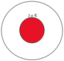
Figure 1: Integration over the red region gives $\Psi_{h,\epsilon}$. Taking $\epsilon\to 0$ gives $Z[J]$. Outer boundary is at $z=0$

The Wilsonian picture on the other hand is (4.5) and describes the situation in Figure 2. The blue region has high momentum modes which are integrated over. This gives $\Psi_{l,a}$ and is the standard Wilsonian picture. Taking $a\to\infty$ gives $Z[J]$.

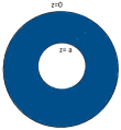
Figure 2: Integration over the blue region gives $\Psi_{l,a}$. Taking $a\to\infty$ gives $Z[J]$.

Both pictures are valid. For actual bulk calculations $\Psi_{h}$ is more useful.

We turn now to an actual calculation.

4.3 Correlation of Scalar Composite using $\Psi_{l}$

4.3.1 ERG equation for Composite Scalar

We will use Polchinski ERG equation in the conventional Wilsonian form involving $\Psi_{l}$ first. In the next section, we repeat using $\Psi_{h}$.

Thus, let us start with a free $O(N)$ vector model like before:

$$Z[J]=\int{\cal D}\phi e^{-\frac{1}{2}\sqrt{N}\int\phi^{I}\Delta^{-1}\phi^{I}+i\int J\phi^{2}},$$ (4.11)

where $\phi^{2}$ stands for $\phi^{I}\phi^{I}$. We have perturbed the (free) CFT by adding a source term for the composite operator $\phi^{2}$. Our strategy will be to introduce an auxiliary field $\sigma$ to represent $\phi^{2}$ and determine an action $S[\sigma]$ that can be used to calculate $\sigma$-correlators using

$$\langle\sigma(x_{1})...\sigma(x_{n})\rangle=\int{\cal D}\sigma~{}\sigma(x_{1})...\sigma(x_{n})~{}e^{-S[\sigma]}$$ (4.12)

The action $S[\sigma]$ can be extracted from

$$Z[J]=\int{\cal D}\phi\int{\cal D}\sigma\delta(\sigma-\phi^{2})e^{-\frac{1}{2}\sqrt{N}\int\phi^{I}\Delta^{-1}\phi^{I}+i\int J\sigma},$$

$$\equiv\int{\cal D}\sigma~{}e^{-S[\sigma]+i\int J\sigma}$$ (4.13)

We will next obtain an ERG equation for determining $S[\sigma]$. To this end we integrate out the modes of $\phi(p)$ with $\Lambda<p<\infty$ as was done in Section 3.1 while deriving the Polchinski ERG equation. This will enable us to define $S_{I,\Lambda}[\sigma,\phi_{l}]$ and an ERG equation for it.

Thus we have, after introducing $\phi_{l},\phi_{h}$ as before,

$$Z[J]= \int{\cal D}\phi_{l}e^{-\frac{1}{2}\sqrt{N}\int\phi^{I}_{l}\Delta_{l}^{-1}\phi^{I}_{l}}\int{\cal D}\phi_{h}\int{\cal D}\sigma e^{i\int J\sigma}\int{\cal D}\chi\exp\bigg{\{}i\int\chi(\sigma-(\phi_{l}+\phi_{h})^{2})$$

$$-\frac{1}{2}\sqrt{N}\int\phi^{I}_{h}\Delta_{h}^{-1}\phi^{I}_{h}\bigg{\}}.$$

One can do the $\phi_{h}$ integral:

$$Z[J]= \int{\cal D}\phi_{l}e^{-\frac{1}{2}\sqrt{N}\int\phi^{I}_{l}\Delta_{l}^{-1}\phi^{I}_{l}}\int{\cal D}\sigma e^{i\int J\sigma}\int{\cal D}\chi~{}e^{i\int\chi\sigma}\int{\cal D}\phi_{h}$$

$$\exp\bigg{\{}-\frac{1}{2}\sqrt{N}\int\phi^{I}_{h}(\Delta_{h}^{-1}+2i\frac{1}{\sqrt{N}}\chi)\phi^{I}_{h}+2i\int\chi\phi^{I}_{l}\phi^{I}_{h}+i\int\chi\phi_{l}^{2}\bigg{\}}$$

$$=\int{\cal D}\phi_{l}e^{-\frac{1}{2}\sqrt{N}\int\phi^{I}_{l}\Delta_{l}^{-1}\phi^{I}_{l}}$$

$$\underbrace{\int{\cal D}\sigma e^{i\int J\sigma}{\cal D}\chi e^{i\int\chi\sigma}\exp\bigg{\{}-\frac{N}{2}Tr\ln(\Delta^{-1}_{h}+2i\frac{1}{\sqrt{N}}\chi)-\frac{1}{2}\int\phi^{I}_{l}\frac{i\chi}{(1+2i\frac{1}{\sqrt{N}}\Delta_{h}\chi)}\phi^{I}_{l}\bigg{\}}}_{e^{-S_{I,\Lambda}[\phi_{l},J]}\equiv\Psi_{l}[\phi_{l},J]}.$$ (4.14)

Polchinski’s ERG equation is, (note that $\dot{\Delta}_{h}=-\dot{\Delta}_{l}$):

$$\frac{\partial\Psi_{l}}{\partial t}=\frac{1}{2}\frac{1}{\sqrt{N}}\int_{p}\dot{\Delta}_{h}(p)\frac{\delta^{2}\Psi_{l}}{\delta\phi^{I}_{l}(p)\delta\phi^{I}_{l}(-p)}.$$ (4.15)

Let us also define $\bar{\Psi}[\phi_{l},\sigma]$ and $\tilde{\Psi}[\phi_{l},\chi]$ as follows:

$$\Psi_{l}[\phi_{l},J]=\int{\cal D}\sigma e^{i\int J\sigma}\bar{\Psi}_{l}[\phi_{l},\sigma]=\int{\cal D}\sigma e^{iJ\sigma}e^{-S_{I,\Lambda}[\phi_{l},\sigma]},$$ (4.16)

so that

$$\bar{\Psi}_{l}[\phi_{l},\sigma]=\int{\cal D}\chi~{}e^{i\int\chi\sigma}\underbrace{\int e^{-\frac{N}{2}Tr\ln(1+2i\frac{1}{\sqrt{N}}\Delta_{h}\chi)-\frac{1}{2}\int\phi^{I}_{l}\frac{i\chi}{(1+2i\frac{1}{\sqrt{N}}\Delta_{h}\chi)}\phi^{I}_{l}}}_{\tilde{\Psi}_{l}[\phi_{l},\chi]}.$$ (4.17)

Thus,

$$\Psi_{l}[\phi_{l},J]=\int{\cal D}\sigma e^{i\int J\sigma}\int{\cal D}\chi~{}e^{i\int\chi\sigma}\tilde{\Psi}_{l}[\phi_{l},\chi]$$

Now we can insert this in (4.15). Thus, we can write

$$\frac{\partial\tilde{\Psi}_{l}}{\partial t}=\frac{1}{2}\frac{1}{\sqrt{N}}\int_{p}\dot{\Delta}_{h}(p)\frac{\delta^{2}\tilde{\Psi}_{l}}{\delta\phi^{I}_{l}(p)\delta\phi^{I}_{l}(-p)}$$ (4.18)

Following [26], we will evaluate this equation at $\phi_{l}=0$. This simplifies things dramatically.

This is

$$\frac{1}{2}\frac{1}{\sqrt{N}}\int_{p}\dot{\Delta}_{h}(p)\frac{\delta^{2}\tilde{\Psi}_{l}}{\delta\phi^{I}_{l}(p)\delta\phi^{I}_{l}(-p)}\Bigg{|}_{\phi_{l}=0}=-\frac{1}{2}\sqrt{N}\int_{p}\dot{\Delta}_{h}(p)\bigg{[}\frac{i\chi}{1+2i\frac{1}{\sqrt{N}}\Delta_{h}\chi}\bigg{]}(p)\tilde{\Psi}_{l}$$

Let us expand this in powers of $\chi$—ignoring the linear term, which comes from a tadpole diagram and can be gotten rid of by shifting the field $\sigma$ [27]. The quadratic and cubic terms are, acting on $\tilde{\Psi}_{l}$:

$$\Big{(}-\int_{k}\int_{p}\dot{\Delta}_{h}(p)\Delta_{h}(k+p)\chi(k)\chi(-k)+$$

$$\frac{2i}{3}\frac{1}{\sqrt{N}}\int\limits_{k_{1},k_{2},k_{3}}\delta(k_{1}+k_{2}+k_{3})\int_{p}\frac{d}{dt}(\Delta_{h}(p)\Delta_{h}(k_{1}+p)\Delta_{h}(k_{1}+k_{2}+p))\chi(k_{1})\chi(k_{2})\chi(k_{3})\Big{)}\tilde{\Psi}_{l}.$$

We can write the quadratic term more suggestively as

$$-\frac{1}{2}\int_{k}\frac{d}{dt}{(\Delta_{h}^{2}(k))}\chi(k)\chi(-k)\tilde{\Psi}_{l}.$$ (4.19)

We get

$$-\frac{1}{2}\int_{k}\chi(k)\chi(-k)\frac{d}{dt}(\Delta_{h}^{2}(k))\tilde{\Psi}_{l}+$$

$$\frac{2i}{3}\frac{1}{\sqrt{N}}\int\limits_{k_{1},k_{2},k_{3}}\delta(k_{1}+k_{2}+k_{3})\int_{p}\frac{d}{dt}(\Delta_{h}(p)\Delta_{h}(p+k_{1})\Delta_{h}(p+k_{1}+k_{2}))\chi(k_{1})\chi(k_{2})\chi(k_{3})\tilde{\Psi}_{l}\Big{|}_{\phi_{l}=0}.$$ (4.20)

This pattern generalizes to higher orders. The $n$th terms are of the form, (a factor $\int_{k_{1},k_{2},...k_{n}}\delta(k_{1}+...+k_{n})$ is understood in each term)

$$N^{\frac{n}{2}-1}\int_{p}\dot{\Delta}_{h}(p)\Delta_{h}(p+k_{1})...\Delta_{h}(p+k_{1}+...k_{n-1})\chi(k_{1})....\chi(k_{n})$$

$$=\frac{2^{n-2}}{n}N^{\frac{n}{2}-1}\int_{p}\frac{d}{dt}\Big{(}\Delta_{h}(p)\Delta_{h}(p+k_{1})...\Delta_{h}(p+k_{1}+...k_{n-1})\Big{)})\chi(k_{1})....\chi(k_{n}).$$

We have used symmetry of the integrand to introduce a factor $1/n$ in the second expression. We thus see that the term multiplying the $n$ external $\chi$’s is a total derivative. This will be important.

Let us proceed now with our analysis of the quadratic and cubic terms. It will be convenient to work with $\bar{\Psi}[\phi_{l},\sigma]$ (defined in (4.17)) in which we can replace $\chi$ by $-i\frac{\delta}{\delta\sigma}$. Converting $\chi\to-i\frac{\delta}{\delta\sigma}$ we get:

$$\frac{\partial\bar{\Psi}_{l}[\phi_{l},\sigma]}{\partial t}\Bigg{|}_{\phi_{l}=0}=\frac{1}{2}\int_{k}\frac{d}{dt}(\Delta_{h}^{2}(k))\frac{\delta^{2}}{\delta\sigma(k)\delta\sigma(-k)}\bar{\Psi}_{l}[\phi_{l},\sigma]|_{\phi_{l}=0}-$$

$$\frac{2}{3\sqrt{N}}\int\limits_{k_{1},k_{2},k_{3}}\delta(k_{1}+k_{2}+k_{3})\frac{d}{dt}\Big{(}\int_{p}\Delta_{h}(p)\Delta_{h}(p+k_{1})\Delta_{h}(p+k_{1}+k_{2})\Big{)}\frac{\delta^{3}\bar{\Psi}_{l}[\phi_{l},\sigma]}{\delta\sigma(k_{1})\delta\sigma(k_{2})\delta\sigma(k_{3})}\Bigg{|}_{\phi_{l}=0}.$$ (4.21)

We see that the propagator for the composite $\sigma$ is $\Delta_{h}^{2}$ as expected.

Let us pause and check whether the leading order term in $\bar{\Psi}$ satisfies this equation. From (4.16), we have

$$\bar{\Psi}_{l}|_{\phi_{l}=0}=\int{\cal D}\chi e^{i\int\chi\sigma}e^{\int_{k}\chi(k)\chi(-k)\Delta_{h}^{2}(k)}=e^{-\frac{1}{2}\int_{k}\frac{\sigma(k)\sigma(-k)}{\Delta_{h}^{2}(k)}}.$$ (4.22)

We have dropped field independent terms. This clearly satisfies the equation (4.21) to leading order.

Acting on the leading order $\bar{\Psi}_{l}$ we can write the second term as a cubic monomial in $\sigma$:

$$-\frac{2}{3}\frac{1}{\sqrt{N}}\int\limits_{k_{1},k_{2},k_{3}}\delta(k_{1}+k_{2}+k_{3})\frac{d}{dt}\Big{(}\int_{p}\Delta_{h}(p)\Delta_{h}(p+k_{1})\Delta_{h}(p+k_{1}+k_{2})\Big{)}$$

$$\times\frac{\delta^{3}}{\delta\sigma(k_{1})\delta\sigma(k_{2})\delta\sigma(k_{3})}\bar{\Psi}_{l}|_{\phi_{l}=0}$$

$$=\frac{2}{3}\frac{1}{\sqrt{N}}\int\limits_{k_{1},k_{2},k_{3}}\delta(k_{1}+k_{2}+k_{3})\frac{d}{dt}\Big{(}\int_{p}\Delta_{h}(p)\Delta_{h}(p+k_{1})\Delta_{h}(p+k_{1}+k_{2})\Big{)}$$

$$\times\frac{\sigma(k_{1})}{\Delta_{h}^{2}(k_{1})}\frac{\sigma(k_{2})}{\Delta_{h}^{2}(k_{2})}\frac{\sigma(k_{3})}{\Delta_{h}^{2}(k_{3})}\bar{\Psi}_{l}|_{\phi_{l}=0}$$

$$\equiv\frac{1}{\sqrt{N}}\int\limits_{k_{1},k_{2},k_{3}}\delta(k_{1}+k_{2}+k_{3})g(k_{1},k_{2},k_{3},\Lambda)\sigma(k_{1})\sigma(k_{2})\sigma(k_{3}).$$ (4.23)

Thus, the ERG equation becomes to this order

$$\frac{\partial\bar{\Psi}_{l}}{\partial t}\bigg{|}_{\phi_{l}=0}= \Big{(}\int_{k}\dot{G}_{s}(k)\frac{\delta^{2}}{\delta\sigma(k)\delta\sigma(-k)}$$

$$+\frac{1}{\sqrt{N}}\int\limits_{k_{1},k_{2},k_{3}}\delta(k_{1}+k_{2}+k_{3})g(k_{1},k_{2},k_{3},\Lambda)\sigma(k_{1})\sigma(k_{2})\sigma(k_{3})\Big{)}\bar{\Psi}_{l}|_{\phi_{l}=0},$$ (4.24)

where

$$g(k_{1},k_{2},k_{3},\Lambda)=\frac{2}{3}\frac{d}{dt}\Big{(}\int_{p}\Delta_{h}(p)\Delta_{h}(p+k_{1})\Delta_{h}(p+k_{1}+k_{2})\Big{)}\frac{1}{G_{s}(k_{1},t)G_{s}(k_{2},t)G_{s}(k_{3},t)}.$$

We have set $\Delta_{h}^{2}=G_{s}$. This determines $\bar{\Psi}_{l}|_{\phi_{l}=0}=e^{-S_{I,\Lambda}[0,\sigma]}$. The leading order expression for $S_{I,\Lambda}[0,\sigma]$ is given in (4.22).

4.3.2 Evolution Operator

The evolution operator for the ERG equation (4.24) can be written as a functional integral:

$$K[\sigma_{f},t_{f};\sigma_{i},t_{i}]= \int\limits_{\sigma(t_{i})=\sigma_{i}}^{\sigma(t_{f})=\sigma_{f}}{\cal D}\sigma~{}\exp\bigg{\{}-\frac{1}{2}\int_{t_{i}}^{t_{f}}dt~{}\bigg{[}\int_{k}\frac{\dot{\sigma}(k,t)\dot{\sigma}(-k,t)}{\dot{G}_{s}(k,t)}$$

$$+\frac{1}{\sqrt{N}}\int\limits_{k_{1},k_{2},k_{3}}\delta(k_{1}+k_{2}+k_{3})g(k_{1},k_{2},k_{3},\Lambda)\sigma(k_{1},t)\sigma(k_{2},t)\sigma(k_{3},t)\bigg{]}\bigg{\}}.$$ (4.25)

The cubic potential term has been added to the action in the path integral, with the $\sigma$ fields becoming functions of $t$.

Let us evaluate it semiclassically, order by order. The leading EOM is

$$\frac{d}{dt}\frac{\dot{\sigma}(-k,t)}{\dot{G}_{s}(k,t)}=0\implies\dot{\sigma}(-k,t)=J(k)\dot{G}_{s}(k,t).$$

Thus,

$$\sigma(k,t)=J(k)G_{s}(k,t),~{}~{}~{}~{}(\because\sigma(k,z=0)=G_{s}(k,z=0)=0).$$ (4.26)

The boundary condition is required—(4.22) is ill-defined at $z=0$ unless $\sigma(k,z=0)$ vanishes.

If we plug this solution into (4.24), one obtains a product of three factors of $\frac{\sigma(k,t)}{G_{s}(k,t)}=J(k)$, which is $t$-independent and the cubic term becomes a total derivative. At one boundary $t=\infty$, where it is non zero, we get

$$\frac{1}{\sqrt{N}}\int_{p}\Delta(p)\Delta(p+k_{1})\Delta(p+k_{1}+k_{2})J(k_{1})J(k_{2})J(k_{3}).$$ (4.27)

This is clearly the correct answer for the one loop contribution of the cubic vertex to the amplitude.

4.4 Correlation of Scalar Composite using $\Psi_{h}$

Given the symmetry $l\leftrightarrow h$ described in (4.6), all the results of the last section can be taken over with $l,h$ interchanged.

Thus, the $\phi_{l}$ fields are integrated over and we get

$$\frac{\partial\bar{\Psi}_{h}}{\partial t}=\frac{1}{2}\int_{k}\frac{d}{dt}(\Delta_{l}^{2}(k))\frac{\delta^{2}}{\delta\sigma(k)\delta\sigma(-k)}\bar{\Psi}_{h}|_{\phi_{h}=0}$$

$$-\frac{2}{3}\frac{1}{\sqrt{N}}\int\limits_{k_{1},k_{2},k_{3}}\delta(k_{1}+k_{2}+k_{3})\frac{d}{dt}\Big{(}\int_{p}\Delta_{l}(p)\Delta_{l}(p+k_{1})\Delta_{l}(p+k_{1}+k_{2})\Big{)}\frac{\delta^{3}}{\delta\sigma(k_{1})\delta\sigma(k_{2})\delta\sigma(k_{3})}\bar{\Psi}_{h}|_{\phi_{h}=0}.$$ (4.28)

(4.22) becomes:

$$\bar{\Psi}_{h}|_{\phi_{h}=0}=\int{\cal D}\chi e^{i\int\chi\sigma}e^{\int_{k}\chi(k)\chi(-k)\Delta_{l}^{2}(k)}=e^{-\frac{1}{2}\int_{k}\frac{\sigma(k)\sigma(-k)}{\Delta_{l}^{2}(k)}}.$$ (4.29)

The Flipped ERG equation is:

$$\frac{\partial\bar{\Psi}_{h}}{\partial t}\bigg{|}_{\phi_{h}=0}= \Big{(}\frac{1}{2}\int_{k}{\dot{G}}_{s}(k)\frac{\delta^{2}}{\delta\sigma(k)\delta\sigma(-k)}$$

$$+\frac{1}{\sqrt{N}}\int\limits_{k_{1},k_{2},k_{3}}\delta(k_{1}+k_{2}+k_{3})g(k_{1},k_{2},k_{3},\Lambda)\sigma(k_{1})\sigma(k_{2})\sigma(k_{3})\Big{)}\bar{\Psi}_{h}\bigg{|}_{\phi_{h}=0},$$ (4.30)

where

$$g(k_{1},k_{2},k_{3},\Lambda)=\frac{2}{3}\frac{d}{dt}\Big{(}\int_{p}\Delta_{l}(p)\Delta_{l}(p+k_{1})\Delta_{l}(p+k_{1}+k_{2})\Big{)}\frac{1}{G_{s}(k_{1},t)G_{s}(k_{2},t)G_{s}(k_{3},t)}.$$

We have set $\Delta_{l}^{2}=G_{s}$. This determines $\bar{\Psi}_{h}|_{\phi_{h}=0}=e^{-S_{I,\Lambda}[\phi_{h}=0,\sigma]}$. The leading order expression for $S_{I,\Lambda}[\phi_{h}=0,\sigma]$ is given in (4.29).

The evolution operator is the same as in (4.25):

$$K[\sigma_{f},t_{f};\sigma_{i},t_{i}]= \int\limits_{\sigma(t_{i})=\sigma_{i}}^{\sigma(t_{f})=\sigma_{f}}{\cal D}\sigma~{}\exp\bigg{\{}-\frac{1}{2}\int_{t_{i}}^{t_{f}}dt~{}\bigg{[}\int_{k}\frac{\dot{\sigma}(k,t)\dot{\sigma}(-k,t)}{\dot{G}_{s}(k,t)}$$

$$+\frac{1}{\sqrt{N}}\int\limits_{k_{1},k_{2},k_{3}}\delta(k_{1}+k_{2}+k_{3})g(k_{1},k_{2},k_{3},\Lambda)\sigma(k_{1},t)\sigma(k_{2},t)\sigma(k_{3},t)\bigg{]}\bigg{\}}.$$ (4.31)

Solving semi classically as before one obtains the same equations, but with the boundary condition that $\sigma$ vanishes at $\infty$ rather than zero, because $\Delta_{l}^{2}$ vanishes at $\Lambda=0$:

$$\frac{d}{dt}\frac{\dot{\sigma}(-k,t)}{\dot{G}_{s}(k,t)}=0\implies\dot{\sigma}(-k,t)=J(k)\dot{G}_{s}(k,t).$$

Thus,

$$\sigma(k,t)=J(k)G_{s}(k,t),~{}~{}~{}~{}(\because\sigma(k,z=\infty)=G_{s}(k,z=\infty)=0).$$ (4.32)

This is the boundary condition used in AdS/CFT correlation function calculations.

The calculation of the correlation function proceeds as before by plugging in this solution into the action. As before, since $\frac{\sigma(k_{i},t)}{G_{s}(k_{i},t)}=J(k_{i})$ is $t$-independent, one obtains again a total derivative, and we pick up the contribution this time, at the $t=-\infty$ ($z=0$) boundary where $\Delta^{2}_{l}=\Delta^{2}$ and the same final answer is obtained:

$$\frac{1}{\sqrt{N}}\int_{p}\Delta(p)\Delta(p+k_{1})\Delta(p+k_{1}+k_{2})J(k_{1})J(k_{2})J(k_{3}).$$ (4.33)

5 Locality of Interaction Term and Mapping to AdS

In the following, we work with the action resulting from the flipped ERG equation.The $D+1$ dimensional action in (4.31) has a non-standard kinetic term and following [24, 26] we will perform a field redefinition that maps it to an action in $AdS_{D+1}$ with the usual scalar kinetic term in $AdS_{D+1}$.

The redefinition is

$$\sigma(p,t)=f(p,t)y(p,t),$$ (5.1)

with

$$\frac{1}{f}=z^{\frac{D}{2}}(A(p)K_{\nu}(pz)-B(p)I_{\nu}(pz)),$$ (5.2)

where $\nu=|\Delta-D/2|$, $\Delta=D-2$ being the dimension of the boundary operator $\sigma(x,0)$. Near the boundary $z=\epsilon$, the leading $z$ behaviour of $y$ is

$$y(p,z)\sim\Big{(}\frac{z}{\epsilon}\Big{)}^{\Delta}\sigma(p,\epsilon).$$ (5.3)

Near the boundary $z\to\epsilon$, $f\to\epsilon^{-\Delta}=\epsilon^{-\frac{D}{2}+\nu}$. Then

$$A(p)=\frac{1}{\Gamma(\nu)}2^{1-\nu}\epsilon^{-\frac{D}{2}+\nu}p^{\nu}.$$ (5.4)

Then we get

$$\frac{1}{f}=\frac{1}{\Gamma(\nu)}2^{1-\nu}\epsilon^{-\frac{D}{2}+\nu}p^{\nu}z^{\frac{D}{2}}K_{\nu}(pz)-\frac{1}{\gamma}2^{\nu-1}\Gamma(\nu)\epsilon^{\frac{D}{2}-\nu}p^{\nu}z^{\frac{D}{2}}I_{\nu}(pz).$$ (5.5)

The Green function $G_{s}$ in turn is given by

$$G_{s}(p,z)=\frac{\gamma^{2}p^{-2\nu}K_{\nu}(pz)}{\gamma K_{\nu}(pz)-2^{2\nu-2}\Gamma(\nu)^{2}\epsilon^{\frac{D}{2}-2\nu}p^{-4\nu}I_{\nu}(pz)}.$$ (5.6)

It vanishes as $z\to\infty$, and

$$G_{s}\to\gamma p^{-2\nu},~{}~{}~{}~{}~{}~{}~{}~{}~{}pz\to 0$$

with $\gamma$ a normalization factor.

The combination $f/G_{s}$ occurs in some calculations below and is given by

$$\frac{f}{G_{s}}=\Gamma(\nu)2^{-1+\nu}\epsilon^{\frac{D}{2}-\nu}z^{-\frac{D}{2}}\frac{p^{\nu}}{\gamma K_{\nu}(pz)}.$$ (5.7)

Kinetic Term

The kinetic term in (4.31) is

$$-\frac{1}{2}\int_{t_{i}}^{t_{f}}dt~{}\int_{p}~{}\frac{\dot{\sigma}(p,t)\dot{\sigma}(-p,t)}{\dot{G}_{s}(p,t)}.$$ (5.8)

Making the field redefinition (5.1) with $f$ given by (5.2) converts it to

$$S_{0}=\frac{1}{2}\int dz~{}\int_{p}~{}z^{-D+1}[\partial_{z}y(p,z)\partial_{z}y(-p,z)+(p^{2}+\frac{m^{2}}{z^{2}})y(p,z)y(-p,z)],$$ (5.9)

with $m^{2}=\nu^{2}-\frac{D^{2}}{4}=4-2D$.

Now we proceed to the interaction term.

Interaction Term

$$S_{I}=\frac{1}{\sqrt{N}}\int dt~{}\int\limits_{k_{1},k_{2},k_{3}}\delta(k_{1}+k_{2}+k_{3})g(k_{1},k_{2},k_{3})\sigma(k_{1},t)\sigma(k_{2},t)\sigma(k_{3},t),$$ (5.10)

with

$$g(k_{1},k_{2},k_{3},\Lambda)=\frac{2}{3}\frac{d}{dt}\Big{(}\int_{p}\Delta_{l}(p)\Delta_{l}(p+k_{1})\Delta_{l}(p+k_{1}+k_{2})\Big{)}\frac{1}{G_{s}(k_{1},t)G_{s}(k_{2},t)G_{s}(k_{3},t)}.$$ (5.11)

We can now substitute (5.1) into (5.10). We will also perform one simplification. Consider the integral

$$I(k_{1},k_{2},\Lambda)=\int_{p}\Delta_{l}(p)\Delta_{l}(p+k_{1})\Delta_{l}(p+k_{1}+k_{2}).$$

We have seen that when the on shell action is used to evaluate the correlation function, only the boundary value of $I$, namely when $\Lambda=\Lambda_{0}\to\infty$, enters the final answer. Thus we have the freedom to choose any regularization procedure for evaluating $I$ as long as it gives the correct answer when $\Lambda=\Lambda_{0}\to\infty$. So we use this freedom and modify the regulator in $g(k_{1},k_{2},k_{3},\Lambda)$. Thus let us choose a regulator and define

$$I_{modified}=\bigg{[}\int_{p}\Delta(p)\Delta(p+k_{1})\Delta(p+k_{1}+k_{2})\bigg{]}_{regulated,\Lambda}.$$

In this particular case, (near $D=3$), one can take $\Lambda\to\Lambda_{0}\to\infty$ and the result is finite. It is clear that this differs from the ERG prescription by $O(\frac{k_{i}}{\Lambda})$, i.e.,

$$I_{modified}=I+O(\frac{k_{i}}{\Lambda}).$$

Since only the value of $I$ at $\Lambda=\Lambda_{0}\to\infty$ enters the final result, the error in the correlation function is $\frac{k_{i}}{\Lambda_{0}}$ and goes to zero as $\Lambda_{0}\to\infty$. Thus we are free to use any $I_{modified}$.

Now the interaction term becomes

$$\frac{2}{3}\frac{1}{\sqrt{N}}\int dt~{}\int_{k_{1},k_{2},k_{3}}\delta(k_{1}+k_{2}+k_{3})\frac{d}{dt}\Big{(}\Big{[}\int_{p}\Delta(p)\Delta(p+k_{1})\Delta(p+k_{1}+k_{2})\Big{]}_{regulated,\Lambda}\Big{)}$$

$$\times\frac{f(k_{1},t)f(k_{2},t)f(k_{3},t)}{G_{s}(k_{1},t)G_{s}(k_{2},t)G_{s}(k_{3},t)}\times y(k_{1},t)y(k_{2},t)y(k_{3},t).$$ (5.12)

The integral has been evaluated in the appendix C for a convenient and commonly used form of the regulator, and one finds:

$$\frac{dI_{modified}}{dt}= \frac{d}{dt}\Big{[}\int_{p}\Delta(p)\Delta(p+k_{1})\Delta(p+k_{1}+k_{2})\Big{]}_{regulated,\Lambda}$$

$$= {\cal N}\frac{K_{\nu}(k_{1}z)}{k_{1}^{\nu}}\frac{K_{\nu}(k_{2}z)}{k_{2}^{\nu}}\frac{K_{\nu}(k_{3}z)}{k_{3}^{\nu}}z^{2(D-3)+3\nu},$$

where $\cal N$ is some numerical constant. The value of $f/G_{s}$ is given in (5.7). Plugging all this into (5.12), one finds that there is an exact cancellation of all momentum dependence! The interaction is local

$$S_{I}={\cal N^{\prime}}\int dt~{}\int_{k_{1},k_{2},k_{3}}\delta(k_{1}+k_{2}+k_{3})y(k_{1},t)y(k_{2},t)y(k_{3},t),$$ (5.13)

with possible cutoff dependence of order $\frac{p}{\Lambda_{0}}$ where $\Lambda_{0}\to\infty$ is the bare cutoff which is to be taken to infinity . The precise form of $f/G_{s}$ in (5.7) was required for this to happen. Thus the nonlocal factor coming from the conformal momentum integrals is exactly compensated for by the function $f/G_{s}$ only when the map is to AdS space.

This concludes our discussion of the cubic scalar vertex. The same logic and techniques will be used for the scalar-scalar-spin 2 vertex. There is a subtlety that needs to be considered before we can do field redefinitions for both scalar and the tensor simultaneously. This is discussed in detail in appendix B.

6 Graviton Coupling

In this section we calculate the cubic correction, involving one spin-2 composite and two scalars, to the ERG equation for the scalar composites in the $O(N)$ model. We will repeat the procedure described in [26] mutatis mutandis.

6.1 Scalar and Tensor auxiliary fields in the Bare action

We work around the Gaussian fixed point as in [38] for simplicity. The free massless spin-2 kinetic term in AdS background was obtained there, starting from the ERG equation for the action for the auxiliary field that stood for the energy momentum tensor composite operator. An auxiliary field standing for the scalar composite will also be introduced. This, in turn, is very similar to the calculation in [26] except that the Wilson-Fisher fixed point action was used there.

Our starting point is thus a generating function

$$Z[J,h^{\mu\nu}]=\int{\cal D}\phi~{}e^{-\frac{1}{2}\int\phi^{I}\Delta^{-1}\phi^{I}-S_{B,I}[\phi,J,h^{\mu\nu}]}.$$ (6.1)

$\Delta$ is a UV regulated propagator of the bare theory with a cutoff $\Lambda_{0}$. $J$ is a source for the composite $\phi^{2}$ and $h^{\mu\nu}$ is a background metric that can be used to define the energy momentum tensor $T_{\mu\nu}$. For the free theory we take

$$S_{B,I}=-i\int J\phi^{2}-i\int h^{\mu\nu}T_{\mu\nu}[\phi].$$ (6.2)

$T_{\mu\nu}[\phi]$ is the traceless and conserved energy momentum tensor of the free theory. It is given by

$$T_{\mu\nu}[\phi]=\partial_{\mu}\phi^{I}\partial_{\nu}\phi^{I}-\frac{1}{2}\delta_{\mu\nu}\partial_{\alpha}\phi^{I}\partial^{\alpha}\phi^{I}-\frac{D-2}{4(D-1)}(\partial_{\mu}\partial_{\nu}-\delta_{\mu\nu}\Box)\phi^{2},$$ (6.3)

and satisfies

$$\partial^{\mu}T_{\mu\nu}[\phi]=T^{\mu}_{~{}\mu}[\phi]=0.$$ (6.4)

We can then restrict $h^{\mu\nu}$ by the “gauge” choice:

$$\partial_{\mu}h^{\mu\nu}=h^{\mu}_{~{}\mu}=0.$$ (6.5)

Once these constraints are imposed on $h^{\mu\nu}$ it follows that only the first term in the expression (6.3) for the energy momentum tensor participates in all further computations.

Introduce auxiliary fields $\sigma,\sigma_{\mu\nu}$ via delta functions

$$\int{\cal D}\sigma\int{\cal D}\sigma_{\mu\nu}~{}\delta(\sigma-\phi^{2})\delta(\sigma_{\mu\nu}-T_{\mu\nu}[\phi])=1,$$

and $\chi,\chi^{\mu\nu}$, Lagrange multiplier fields to implement the delta functions. Because of (6.4)

$$\partial^{\mu}\sigma_{\mu\nu}=\sigma^{\mu}_{~{}\mu}=0,$$ (6.6)

and because of (6.5) $\chi^{\mu\nu}$ can also be chosen to satisfy

$$\partial_{\mu}\chi^{\mu\nu}=\chi^{\mu}_{~{}\mu}=0.$$ (6.7)

Then

$$Z[J,h^{\mu\nu}]$$

$$=\int{\cal D}\phi\int{\cal D}\sigma\int{\cal D}\chi e^{i\int\chi(\sigma-\phi^{2})}\int{\cal D}\sigma_{\mu\nu}\int{\cal D}\chi^{\mu\nu}e^{i\int\chi^{\mu\nu}(\sigma_{\mu\nu}+i\frac{\delta}{\delta h^{\mu\nu}})}~{}e^{-\frac{1}{2}\sqrt{N}\int\phi^{I}\Delta^{-1}\phi^{I}-S_{B,I}[\phi,J,h^{\mu\nu}]}$$

$$=\int{\cal D}\phi~{}e^{-\frac{1}{2}\sqrt{N}\int\phi^{I}\Delta^{-1}\phi^{I}}\int{\cal D}\sigma\int{\cal D}\chi\int{\cal D}\sigma_{\mu\nu}\int{\cal D}\chi^{\mu\nu}e^{i\int\chi\sigma}e^{i\int\chi^{\mu\nu}\sigma_{\mu\nu}}e^{i\int(J-\chi)\phi^{2}+i\int(h^{\mu\nu}-\chi^{\mu\nu})T_{\mu\nu}[\phi]}.$$

Redefining $\chi-J\to\chi,~{}~{}\chi^{\mu\nu}-h^{\mu\nu}\to\chi^{\mu\nu}$, we ge

$$Z[J,h^{\mu\nu}]=\int{\cal D}\sigma~{}e^{i\int J\sigma}\int{\cal D}\sigma_{\mu\nu}~{}e^{i\int h^{\mu\nu}\sigma_{\mu\nu}}$$

$$\underbrace{\int{\cal D}\chi\int{\cal D}\chi^{\mu\nu}\int{\cal D}\phi~{}e^{-\frac{1}{2}\sqrt{N}\int\phi^{I}\Delta^{-1}\phi^{I}}~{}e^{i\int\chi\sigma}e^{i\int\chi^{\mu\nu}\sigma_{\mu\nu}}e^{-i\int\chi\phi^{2}-i\int\chi^{\mu\nu}T_{\mu\nu}[\phi]}}_{e^{-S[\sigma,\sigma_{\mu\nu}]}}.$$ (6.8)

$S[\sigma,\sigma_{\mu\nu}]$ is the action for the auxiliary fields obtained after integrating out $\phi$. It can be used to evaluate correlation functions of the composite operators. For instance,

$$\int{\cal D}\sigma\int{\cal D}\sigma_{\mu\nu}~{}\sigma_{\mu\nu}(x)\sigma_{\rho\sigma}(y)e^{-S[\sigma,\sigma_{\mu\nu}]}=\langle T_{\mu\nu}[\phi](x)T_{\mu\nu}[\phi](y)\rangle.$$ (6.9)

6.2 Wilson Action

We now proceed to integrate out just the high energy modes of $\phi(p),~{}\Lambda_{0}>p>\Lambda$ (with $\Lambda_{0}\to\infty$) and thus obtain the Wilson action. Thus using standard methods [36] we write

$$\phi=\phi_{l}+\phi_{h};~{}~{}~{}~{}~{}~{}~{}~{}~{}\Delta=\Delta_{l}+\Delta_{h}.$$

The low energy propagator, $\Delta_{l}$ propagates modes with $0<p<\Lambda$ and the high energy propagator $\Delta_{h}$ propagates modes with $\Lambda<p<\infty$.

$$Z[J,h_{\mu\nu}]=\int{\cal D}\sigma~{}e^{i\int J\sigma}\int{\cal D}\sigma_{\mu\nu}~{}e^{i\int h^{\mu\nu}\sigma_{\mu\nu}}\int{\cal D}\chi\int{\cal D}\chi^{\mu\nu}$$

$$\int{\cal D}\phi_{l}\int{\cal D}\phi_{h}~{}e^{-\frac{1}{2}\sqrt{N}\int\phi^{I}_{l}\Delta_{l}^{-1}\phi^{I}_{l}-\frac{1}{2}\sqrt{N}\int\phi^{I}_{h}\Delta_{h}^{-1}\phi^{I}_{h}}~{}e^{i\int\chi\sigma}e^{i\int\chi^{\mu\nu}\sigma_{\mu\nu}}e^{-i\int\chi(\phi_{l}+\phi_{h})^{2}-i\int\chi^{\mu\nu}T_{\mu\nu}[\phi_{l}+\phi_{h}]}.$$ (6.10)

The Wilson action is a functional of $\phi_{l}$, (and also $J,h_{\mu\nu}$), and is obtained by integrating out $\phi_{h}$. Thus, let us write

$$e^{-S_{\Lambda}[\phi_{l},J,h_{\mu\nu}]}= e^{-\frac{1}{2}\sqrt{N}\int\phi^{I}_{l}\Delta^{-1}\phi^{I}_{l}}\int{\cal D}\sigma~{}e^{i\int J\sigma}\int{\cal D}\sigma_{\mu\nu}~{}e^{i\int h^{\mu\nu}\sigma_{\mu\nu}}\int{\cal D}\chi\int{\cal D}\chi^{\mu\nu}$$

$$\int{\cal D}\phi_{h}~{}e^{-\frac{1}{2}\sqrt{N}\int\phi^{I}_{h}\Delta_{h}^{-1}\phi^{I}_{h}}~{}e^{i\int\chi\sigma}e^{i\int\chi^{\mu\nu}\sigma_{\mu\nu}}e^{-i\int\chi(\phi_{l}+\phi_{h})^{2}-i\int\chi^{\mu\nu}T_{\mu\nu}[\phi_{l}+\phi_{h}]}$$

$$= e^{-\frac{1}{2}\sqrt{N}\int\phi^{I}_{l}\Delta^{-1}\phi^{I}_{l}}e^{-S_{I,\Lambda}[\phi_{l},J,h^{\mu\nu}]}.$$ (6.11)

Thus,

$$e^{-S_{I,\Lambda}[\phi_{l},J,h^{\mu\nu}]}=\int{\cal D}\sigma\int{\cal D}\sigma_{\mu\nu}e^{i\int J\sigma+i\int h^{\mu\nu}\sigma_{\mu\nu}}e^{-S_{I,\Lambda}[\phi_{l},\sigma,\sigma_{\mu\nu}]}.$$ (6.12)

$S_{I,\Lambda}[\phi_{l},J,h^{\mu\nu}]$ as well as its Fourier transfrom $S_{I,\Lambda}[\phi_{l},\sigma,\sigma_{\mu\nu}]$ obey Polchinski ERG equation, which describes their evolution as $\Lambda$ is taken to zero. Thus $S[\sigma,\sigma_{\mu\nu}]$ used in (6.9) is defined as

$$S[\sigma,\sigma_{\mu\nu}]=\lim_{\Lambda\to 0}S_{I,\Lambda}[\phi_{l}=0,\sigma,\sigma_{\mu\nu}].$$

Let us focus on the $\phi_{h}$ integration first, treating the other fields as background fields. Define

$$e^{-\tilde{S}_{I,\Lambda}[\phi_{l},\chi,\chi^{\mu\nu}]}=\int{\cal D}\phi_{h}e^{-\frac{1}{2}\sqrt{N}\int\phi^{I}_{h}\Delta_{h}^{-1}\phi^{I}_{h}}e^{-\tilde{S}_{I,\Lambda}[\phi_{l},\phi_{h},\chi,\chi^{\mu\nu}]}$$

$$=\int{\cal D}\phi_{h}~{}e^{-\frac{1}{2}\sqrt{N}\int\phi^{I}_{h}\Delta_{h}^{-1}\phi^{I}_{h}}~{}e^{-i\int\chi(\phi_{l}+\phi_{h})^{2}-i\int\chi^{\mu\nu}T_{\mu\nu}[\phi_{l}+\phi_{h}]}.$$

Then

$$e^{-S_{I,\Lambda}[\phi_{l},\sigma,\sigma_{\mu\nu}]}=\int{\cal D}\chi\int{\cal D}\chi^{\mu\nu}e^{i\int\chi\sigma+i\int\chi^{\mu\nu}\sigma_{\mu\nu}-\tilde{S}_{I,\Lambda}[\phi_{l}.\chi,\chi^{\mu\nu}]}.$$ (6.13)

6.3 Doing the $\phi_{h}$ integral

Let us isolate the various types of terms in $\tilde{S}_{I,\Lambda}[\phi_{l},\phi_{h},\chi,\chi^{\mu\nu}]$:

1. Quadratic in $\phi_{h}$

   $$\tilde{S}_{I,\Lambda,hh}= \int_{x}\int_{y}\Big{[}\frac{1}{2}\sqrt{N}\phi^{I}_{h}(x)\Delta_{h}^{-1}(x,y)\phi^{I}_{h}(y)$$

   $$+i\phi^{I}_{h}(x)\chi(x)\delta(x-y)\phi^{I}_{h}(y)+i\phi^{I}_{h}(x)\chi^{\mu\nu}(x)\Theta_{\mu\nu}\delta(x-y)\phi^{I}_{h}(y)\Big{]},$$ (6.14)

   where $\Theta_{\mu\nu}$ is defined as the differential operator contained in $T_{\mu\nu}$, cf. (6.3):

   $$T_{\mu\nu}(x)\equiv\phi^{I}(x)\Theta_{\mu\nu}(x)\phi^{I}(x).$$ (6.15)

   We write this as

   $$\tilde{S}_{\Lambda,hh}=\frac{1}{2}\int_{x}\int_{y}\phi^{I}_{h}(x)O^{-1}(x,y)\phi^{I}_{h}(y),$$ (6.16)

   with

   $$O^{-1}(x,y)=\sqrt{N}\Delta_{h}^{-1}(x,y)+\underbrace{2i\chi(x)\delta(x-y)}_{A}+\underbrace{2i\chi^{\mu\nu}(x)\Theta_{\mu\nu}\delta(x-y)}_{B}.$$

2. Quadratic in $\phi_{l}$

   $$\tilde{S}_{I,\Lambda,ll}=i\int\chi\phi_{l}^{2}+i\int\chi^{\mu\nu}\phi^{I}_{l}\Theta_{\mu\nu}\phi^{I}_{l}$$

   $$=i\int_{x}\int_{y}~{}\phi^{I}_{l}(x)\Big{[}\chi(x)\delta(x-y)+\chi^{\mu\nu}(x)\Theta_{\mu\nu}\delta(x-y)\Big{]}\phi^{I}_{l}(y)$$ (6.17)

   $$=\frac{1}{2}\int_{x}\int_{y}\phi^{I}_{l}(A+B)\phi^{I}_{l}.$$

3. Linear in $\phi_{l},\phi_{h}$

   $$\tilde{S}_{I,\Lambda,lh}=2i\int\chi\phi^{I}_{l}\phi^{I}_{h}+i\int\chi^{\mu\nu}(\phi^{I}_{l}\Theta_{\mu\nu}\phi^{I}_{h}+\phi^{I}_{h}\Theta_{\mu\nu}\phi^{I}_{l})$$

   $$=2i\int_{y}\int_{x}\phi^{I}_{l}(x)\Big{[}\chi(x)\delta(x-y)+\chi^{\mu\nu}\Theta_{\mu\nu}\delta(x-y)\Big{]}\phi^{I}_{h}(y)$$

   $$=\int_{x}\int_{y}\phi^{I}_{l}(A+B)\phi^{I}_{h}.$$

   $$\equiv\int_{y}j^{I}(y)\phi^{I}_{h}(y).$$ (6.18)

   We have integrated by parts and used $\partial_{\mu}\chi^{\mu\nu}=0$.

   Now we can do the $\phi_{h}$ integral in

   $$\int{\cal D}\phi_{h}e^{-\frac{1}{2}\int_{x}\int_{y}\phi^{I}_{h}O^{-1}(x,y)\phi^{I}_{h}(y)-\int_{x}j^{I}(x)\phi^{I}_{h}(x)}$$

   $$=e^{\frac{N}{2}Tr\ln O+\frac{1}{2}\int_{x}\int_{y}j^{I}(x)O(x,y)j^{I}(y)}.$$

   Thus we obtain

   $$\tilde{S}_{I,\Lambda}[\phi_{l},\chi,\chi^{\mu\nu}]=i\int_{x}\int_{y}~{}\phi^{I}_{l}(x)\Big{[}\chi(x)\delta(x-y)+\chi^{\mu\nu}(x)\Theta_{\mu\nu}\delta(x-y)\Big{]}\phi^{I}_{l}(y)$$

   $$-\frac{N}{2}Tr\ln O-\frac{1}{2}\int_{x}\int_{y}j^{I}(x)O(x,y)j^{I}(y).$$ (6.19)

6.4 ERG Equation

If we let $\tilde{\Psi}=e^{-\tilde{S}_{I,\Lambda}[\phi_{l},\chi,\chi^{\mu\nu}]}$ then Polchinski’s ERG equation is:

$$\frac{\partial\tilde{\Psi}}{\partial t}=-\frac{1}{2}\frac{1}{\sqrt{N}}\int_{p}\dot{\Delta}_{l}(p)\frac{\delta^{2}\tilde{\Psi}}{\delta\phi^{I}_{l}(p)\delta\phi^{I}_{l}(-p)}.$$ (6.20)

Following [26] we will evaluate this equation at $\phi_{l}=0$. This simplifies the equation considerably. The disadvantage is that we cannot integrate out any more $\phi_{l}$ modes. This means $\Lambda$ is a physical IR cutoff in the problem. Thus to recover the physics, one has to set $\Lambda=0$. Once we have a general solution valid for arbitrary $\Lambda$ this is not difficult to do.

This procedure gives us an equation for $\tilde{S}_{I,\Lambda}[0,\chi,\chi^{\mu\nu}]$ and after integrating over $\chi,\chi^{\mu\nu}$ as in (6.13), an equation for $S_{I,\Lambda}[0,\sigma,\sigma_{\mu\nu}]$.

Define $\Psi=e^{-\tilde{S}_{I,\Lambda}[\phi_{l},\sigma,\sigma^{\mu\nu}]}=\int{\cal D}\chi\int{\cal D}\chi^{\mu\nu}e^{i\int\chi\sigma+i\int\chi^{\mu\nu}\sigma_{\mu\nu}}\tilde{\Psi}$ as in (6.13). Then (6.20), on setting $\phi_{l}=0$, immediately leads to

$$\frac{\partial\Psi}{\partial t}\bigg{|}_{\phi_{l}=0}=-\frac{1}{2}\frac{1}{\sqrt{N}}\int_{p}\dot{\Delta}_{l}(p)\frac{\delta^{2}\Psi}{\delta\phi^{I}_{l}(p)\delta\phi^{I}_{l}(-p)}\bigg{|}_{\phi_{l}=0}.$$ (6.21)

Since $\dot{\Delta}_{l}=-\dot{\Delta}_{h}$ we can write an equivalent equation:

$$\frac{\partial\Psi}{\partial t}\bigg{|}_{\phi_{l}=0}=\frac{1}{2}\frac{1}{\sqrt{N}}\int_{p}\dot{\Delta}_{h}(p)\frac{\delta^{2}\Psi}{\delta\phi^{I}_{l}(p)\delta\phi^{I}_{l}(-p)}\bigg{|}_{\phi_{l}=0}.$$ (6.22)

This is a more useful form since the propagator that appears in $\Psi$ is $\Delta_{h}$, (see (6.14)).

Let us evaluate the RHS of this equation.

$$O^{-1}=\sqrt{N}\frac{1}{\Delta_{h}}+A+B=\sqrt{N}\Delta_{h}^{-1}(I+\frac{1}{\sqrt{N}}\Delta_{h}A+\frac{1}{\sqrt{N}}\Delta_{h}B),$$

$$O= \frac{1}{\sqrt{N}}\frac{1}{(I+\frac{1}{\sqrt{N}}\Delta_{h}A+\frac{1}{\sqrt{N}}\Delta_{h}B)}\Delta_{h}$$

$$= \frac{1}{\sqrt{N}}[1-\frac{1}{\sqrt{N}}(\Delta_{h}A+\Delta_{h}B)+\frac{1}{N}(\Delta_{h}A+\Delta_{h}B)^{2}+...]\Delta_{h},$$

$$\frac{1}{2}j^{I}Oj^{I}=\frac{1}{2}\frac{1}{\sqrt{N}}\phi^{I}_{l}(A+B)[1-\frac{1}{\sqrt{N}}(\Delta_{h}A+\Delta_{h}B)+\frac{1}{N}(\Delta_{h}A+\Delta_{h}B)^{2}+...]\Delta_{h}(A+B)\phi^{I}_{l}.$$

We have to add $\frac{1}{2}\phi^{I}_{l}(A+B)\phi^{I}_{l}$ from (6.17).

$$\frac{1}{2}\frac{1}{\sqrt{N}}\int_{p}\dot{\Delta}_{h}(p)\frac{\delta^{2}\tilde{\Psi}}{\delta\phi^{I}_{l}(p)\delta\phi^{I}_{l}(-p)}|_{\phi_{l}=0}=$$

$$\frac{1}{2}\int_{p}\dot{\Delta}_{h}\{\sqrt{N}(A+B)+(A+B)[1-\frac{1}{\sqrt{N}}(\Delta_{h}A+\Delta_{h}B)+\frac{1}{N}(\Delta_{h}A+\Delta_{h}B)^{2}+...]\Delta_{h}(A+B)\}\tilde{\Psi}.$$

We are interested in the terms involving two $\chi$’s and one $\chi^{\mu\nu}$ . This will generate the required cubic term as will become clear below. This comes from

$$\frac{1}{\sqrt{N}}\dot{\Delta}_{h}\{A[-\Delta_{h}B]\Delta_{h}A+B[-\Delta_{h}A]\Delta_{h}A+A[-\Delta_{h}A]\Delta_{h}B\}.$$

This can be written compactly in position space:

$$4i\frac{1}{\sqrt{N}}\frac{d}{dt}\int\limits_{x,y,z}\chi(x)\Delta_{h}(x-y)\chi(y)\Delta_{h}(y-z)\chi^{\mu\nu}(z)\frac{\partial^{2}}{\partial z^{\mu}\partial z^{\nu}}\Delta_{h}(z-x).$$

Acting on $\Psi=e^{-S_{I,\Lambda}[\sigma,\sigma^{\mu\nu},\phi_{l}=0]}$ this term becomes

$$-4\frac{1}{\sqrt{N}}\int\limits_{x,y,z}\frac{d}{dt}\Big{(}(\Delta_{h}(x-y)\Delta_{h}(y-z)\frac{\partial^{2}}{\partial z^{\mu}\partial z^{\nu}}\Delta_{h}(z-x))\Big{)}\frac{\delta^{3}e^{-S_{I,\Lambda}[\sigma,\sigma^{\mu\nu},\phi_{l}=0]}}{\delta\sigma(x)\delta\sigma(y)\delta\sigma_{\mu\nu}(z)}.$$ (6.23)

The Feynman diagram corresponding to this term is given below in figure 3.

Figure 3: scalar-scalar-tensor diagram

We now need to address a problem pointed out in [27]. The scalar propagator $\Delta_{h}^{2}$ and the graviton propagator, which is proportional to $(\partial^{2})^{2}\Delta_{h}^{2}$, cannot be simultaneously mapped to AdS space. One of them (tensor) should have $\nu=-\frac{D}{2}$ and the other needs to have $\nu=-\frac{D}{2}+2$. These conditions are mutually incompatible. A resolution was suggested in [27]. This is to redefine one of the fields (say, the scalar) by a function $g_{s}$ selected so that the propagator for the scalar is modified. This is worked out in appendix B. Thus we let $\sigma(p)=g(p)\phi^{2}(p)$. Then the scalar propagator becomes $g^{2}\Delta_{h}^{2}$. Then one can choose $g$ such that this has $\nu=-\frac{D}{2}+2$. With this modification (6.23) changes to, (in momentum space now),

$$-4\frac{1}{\sqrt{N}}\int\limits_{k_{1},k_{2},k_{3}}\delta(k_{1}+k_{2}+k_{3})\frac{d}{dt}\Big{(}\int_{p}(\Delta_{h}(p+k_{1}+k_{2})\Delta_{h}(p+k_{1})p^{\mu}p^{\nu}\Delta_{h}(p)g(k_{1})g(k_{2}))\Big{)}$$

$$\times\frac{\delta^{3}}{\delta\sigma(k_{1})\delta\sigma(k_{2})\delta\sigma_{\mu\nu}(k_{3})}e^{-S_{I,\Lambda}[\sigma,\sigma^{\mu\nu},\phi_{l}=0]}.$$ (6.24)

6.5 ERG Equation

In the previous sections we had introduced the auxiliary field $\sigma$ standing for $g\phi^{2}$ and $\sigma_{\mu\nu}$ standing for the energy momentum tensor. The ERG equation for the effective action involving $\sigma$ and $\sigma_{\mu\nu}$ is

$$\frac{\partial\bar{\Psi}_{l}}{\partial t}\bigg{|}_{\phi_{l}=0}=\bigg{\{}\frac{1}{2}\int_{k}\frac{d}{dt}(g(k)^{2}\Delta_{h}^{2}(k))\frac{\delta^{2}}{\delta\sigma(k)\delta\sigma(-k)}+\frac{1}{2}\int_{k}\frac{d}{dt}((k^{2}\Delta_{h})^{2}(k))\frac{\delta^{2}}{\delta\sigma_{\mu\nu}(k)\delta\sigma^{\mu\nu}(-k)}$$

$$-\frac{2}{3}\frac{1}{\sqrt{N}}\int\limits_{k_{1},k_{2},k_{3}}\frac{d}{dt}\Big{(}g(k_{1})g(k_{2})g(k_{3})\int_{p}\Delta_{h}(p)\Delta_{h}(p+k_{1})\Delta_{h}(p+k_{1}+k_{2})\Big{)}\frac{\delta^{3}}{\delta\sigma(k_{1})\delta\sigma(k_{2})\delta\sigma(k_{3})}$$

$$-\frac{4}{\sqrt{N}}\int\limits_{k_{1},k_{2},k_{3}}\frac{d}{dt}\Big{(}\int_{p}(\Delta_{h}(p+k_{1}+k_{2})\Delta_{h}(p+k_{1})p^{\mu}p^{\nu}\Delta_{h}(p)g(k_{1})g(k_{2}))\Big{)}\frac{\delta^{3}}{\delta\sigma(k_{1})\delta\sigma(k_{2})\delta\sigma_{\mu\nu}(k_{3})}\bigg{\}}$$

$$\bar{\Psi}_{l}|_{\phi_{l}=0},$$ (6.25)

where a momentum conserving $\delta(k_{1}+k_{2}+k_{3})$ is implicit in the cubic terms.

The leading order solution is

$$\bar{\Psi}_{l}|_{\phi_{l}=0}=\exp\bigg{\{}-\frac{1}{2}\int_{k}\frac{\sigma(k)\sigma(-k)}{G_{s}(k)}-\frac{1}{2}\int_{k}\frac{\sigma_{\mu\nu}(k)\sigma^{\mu\nu}(-k)}{G_{t}(k)}\bigg{\}},$$

where as before $G_{s}=g^{2}\Delta_{h}^{2}$ and $G_{t}=(k^{2}\Delta_{h})^{2}$. Acting on this, the cubic derivatives give

$$-\frac{\sigma(k_{1})}{G_{s}(k_{1})}\frac{\sigma(k_{2})}{G_{s}(k_{2},t)}\frac{\sigma(k_{3})}{G_{s}(k_{3},t)},$$

and

$$-\frac{\sigma(k_{1})}{G_{s}(k_{1},t)}\frac{\sigma(k_{2})}{G_{s}(k_{2},t)}\frac{\sigma_{\mu\nu}(k_{3})}{G_{t}(k_{3},t)}.$$

These terms add potential terms to the ERG equation.

6.6 Flipped ERG equation

As explained in Section 2 and Section 3 the flipped ERG equation (4.7) is more suited for mapping to AdS. Flipping is easily done—interhange $l\leftrightarrow h$.

Thus, the flipped ERG equation is

$$\frac{\partial\bar{\Psi}_{h}}{\partial t}\bigg{|}_{\phi_{h}=0}=\bigg{\{}\frac{1}{2}\int_{k}\frac{d}{dt}(g(k)^{2}\Delta_{l}^{2}(k))\frac{\delta^{2}}{\delta\sigma(k)\delta\sigma(-k)}+\frac{1}{2}\int_{k}\frac{d}{dt}((k^{2}\Delta_{l})^{2}(k))\frac{\delta^{2}}{\delta\sigma_{\mu\nu}(k)\delta\sigma^{\mu\nu}(-k)}$$

$$-\frac{2}{3}\frac{1}{\sqrt{N}}\int\limits_{k_{1},k_{2},k_{3}}\frac{d}{dt}\Big{(}g(k_{1})g(k_{2})g(k_{3})\int_{p}\Delta_{l}(p)\Delta_{l}(p+k_{1})\Delta_{l}(p+k_{1}+k_{2})\Big{)}\frac{\delta^{3}}{\delta\sigma(k_{1})\delta\sigma(k_{2})\delta\sigma(k_{3})}$$

$$-4\frac{1}{\sqrt{N}}\int\limits_{k_{1},k_{2},k_{3}}\frac{d}{dt}\Big{(}\int_{p}(\Delta_{l}(p+k_{1}+k_{2})\Delta_{l}(p+k_{1})p^{\mu}p^{\nu}\Delta_{l}(p)g(k_{1})g(k_{2}))\Big{)}$$

$$\times\frac{\delta^{3}}{\delta\sigma(k_{1})\delta\sigma(k_{2})\delta\sigma_{\mu\nu}(k_{3})}\bigg{\}}\bar{\Psi}_{h}|_{\phi_{h}=0},$$ (6.26)

with a momentum conserving $\delta(k_{1}+k_{2}+k_{3})$ in the cubic terms.

The leading order solution is

$$\bar{\Psi}_{h}|_{\phi_{h}=0}=\exp\bigg{\{}-\frac{1}{2}\int_{k}\frac{\sigma(k)\sigma(-k)}{G_{s}(k)}-\frac{1}{2}\int_{k}\frac{\sigma_{\mu\nu}(k)\sigma^{\mu\nu}(-k)}{G_{t}(k)}\bigg{\}},$$ (6.27)

where now $G_{s}=g^{2}\Delta_{l}^{2}$ and $G_{t}=(k^{2}\Delta_{l})^{2}$. Acting on this the cubic derivative terms give

$$-\frac{\sigma(k_{1})}{G_{s}(k_{1})}\frac{\sigma(k_{2})}{G_{s}(k_{2},t)}\frac{\sigma(k_{3})}{G_{s}(k_{3},t)},$$

and

$$-\frac{\sigma(k_{1})}{G_{s}(k_{1},t)}\frac{\sigma(k_{2})}{G_{s}(k_{2},t)}\frac{\sigma_{\mu\nu}(k_{3})}{G_{t}(k_{3},t)}.$$

These contribute potential terms to the flipped ERG equation.

7 Mapping Evolution Operator to AdS

The evolution operator for the flipped ERG equation can be written as

$$\int{\cal D}\sigma{\cal D}\sigma_{\mu\nu}~{}\exp\bigg{\{}-\int dt\int_{p}~{}\bigg{[}\frac{1}{2}\frac{\dot{\sigma}\dot{\sigma}}{\dot{G}_{s}}+\frac{1}{2}\frac{\dot{\sigma}_{\mu\nu}\dot{\sigma}^{\mu\nu}}{\dot{G}_{t}}+~{}V(\sigma,\sigma_{\mu\nu})\bigg{]}\bigg{\}}$$

where

$$V(\sigma,\sigma_{\mu\nu})=\frac{1}{\sqrt{N}}\int\limits_{k_{1},k_{2},k_{3}}\delta(k_{1}+k_{2}+k_{3})\times$$

$$\bigg{\{}-\frac{2}{3}\frac{d}{dt}\Big{(}g(k_{1})g(k_{2})g(k_{3})\int_{p}\Delta_{l}(p)\Delta_{l}(p+k_{1})\Delta_{l}(p+k_{1}+k_{2})\Big{)}\Big{(}\frac{\sigma(k_{1},t)}{G_{s}(k_{1},t)}\frac{\sigma(k_{2},t)}{G_{s}(k_{2},t)}\frac{\sigma(k_{3},t)}{G_{s}(k_{3},t)}\Big{)}$$

$$-4\frac{d}{dt}\Big{(}\int_{p}(\Delta_{l}(p+k_{1}+k_{2})\Delta_{l}(p+k_{1})p^{\mu}p^{\nu}\Delta_{l}(p)g(k_{1})g(k_{2}))\Big{)}\Big{(}\frac{\sigma(k_{1},t)}{G_{s}(k_{1},t)}\frac{\sigma(k_{2},t)}{G_{s}(k_{2},t)}\frac{\sigma_{\mu\nu}(k_{3},t)}{G_{t}(k_{3},t)}\Big{)}\bigg{\}}.$$ (7.1)

The scalar part of this was done in Section 3, (without the factor $g$). As shown in Section 3.1, substituting the leading order solution, one sees that the factors $\frac{\sigma(k,t)}{G_{s}(k,t)}$ are all time independent. Then the integrand becomes a total derivative and we recover the expected amplitudes. The important point is that the final amplitude thus depends only on the value of $g\Delta_{l}$ at the limits of the $t$ integration—where it is zero at one end, ($z=\infty$), and $\Delta$ at the other $(z=0)$. As explained in Section 3 we can modify the regularization procedure in each of the loop integrals. The errors in the final answer, viz, correlation function, is of $O(\frac{k_{i}}{\Lambda_{0}})$. In the limit $\Lambda_{0}\to\infty$ there is no error. We use this freedom exactly as it was done in Section 3. Thus $V$ becomes

$$V(\sigma,\sigma_{\mu\nu})=\frac{1}{\sqrt{N}}\int\limits_{k_{1},k_{2},k_{3}}\delta(k_{1}+k_{2}+k_{3})\times$$

$$\bigg{\{}-\frac{2}{3}\frac{d}{dt}\Big{[}\int_{p}\Delta(p)\Delta(p+k_{1})\Delta(p+k_{1}+k_{2})\Big{]}_{regulated,\Lambda}\Big{(}\frac{\sigma(k_{1},t)}{G_{s}(k_{1},t)}\frac{\sigma(k_{2},t)}{G_{s}(k_{2},t)}\frac{\sigma(k_{3},t)}{G_{s}(k_{3},t)}\Big{)}$$

$$-4\frac{d}{dt}\Big{[}\int_{p}(\Delta(p+k_{1}+k_{2})\Delta(p+k_{1})p^{\mu}p^{\nu}\Delta(p))\Big{]}_{regulated,\Lambda}\Big{(}\frac{\sigma(k_{1},t)}{G_{s}(k_{1},t)}\frac{\sigma(k_{2},t)}{G_{s}(k_{2},t)}\frac{\sigma_{\mu\nu}(k_{3},t)}{G_{t}(k_{3},t)}\Big{)}\bigg{\}}.$$ (7.2)

We now map the action to AdS space by the substitution $\sigma=fy$ and $\sigma_{\mu\nu}=fy_{\mu\nu}$. Thus the coefficient of $y(k_{1})y(k_{2})y(k_{3})$ becomes

$$-\frac{2}{3}\frac{d}{dt}\Big{[}\int_{p}\Delta(p)\Delta(p+k_{1})\Delta(p+k_{1}+k_{2})\Big{]}_{regulated,\Lambda}\Big{(}\frac{f(k_{1},t)}{G_{s}(k_{1},t)}\frac{f(k_{2},t)}{G_{s}(k_{2},t)}\frac{f(k_{3},t)}{G_{s}(k_{3},t)}\Big{)}.$$

As mentioned in Section 3, the time derivative of the loop momentum integral with a convenient regularization procedure is,

$$2(k_{1}{\Lambda})^{-\nu_{1}}K_{\nu_{1}}(k_{1}/\Lambda)\times 2({k_{2}}{\Lambda})^{-\nu_{2}}K_{\nu_{2}}(k_{2}/\Lambda)\times 2({k_{3}}{\Lambda})^{-\nu}K_{\nu_{3}}(k_{3}/\Lambda)$$

upto a normalising factor. The factor $\frac{f}{G_{s}}$ was given in [26] and is the inverse of the above expression. Thus there is an exact cancellation, exactly as described in Section 3 for the scalar case, since (5.7)

$$\frac{f(k,z)}{G_{s}(k,z)}=\epsilon^{\frac{D}{2}-\nu}\frac{z^{-D/2}(k)^{\nu}}{K_{\nu}(k/\Lambda)}.$$

So they cancel exactly for the three scalar case and we get a local term up to some normalization.

$${\cal N}\int_{k_{1},k_{2},k_{3}}\delta(k_{1}+k_{2}+k_{3})y(k_{1},\Lambda)y(k_{2},\Lambda)y(k_{3},\Lambda).$$ (7.3)

For the second loop integral, the computation is done in appendix C, resulting in

$$z^{2D-2}\Big{(}\frac{k_{1}}{z}\Big{)}^{-\nu}K_{\nu}(k_{1}z)~{}\Big{(}\frac{k_{2}}{z}\Big{)}^{-\nu}K_{\nu}(k_{2}z)~{}\Big{(}\frac{k_{3}}{z}\Big{)}^{\nu^{\prime}}K_{\nu^{\prime}}(k_{3}z),$$ (7.4)

where $\nu$ and $\nu^{\prime}$ correspond to the scalar and the tensor respectively. For the tensor, (see appendix A),

$$\frac{f_{t}(k,z)}{G_{t}(k,z)}=\epsilon^{\frac{D}{2}-\nu^{\prime}}\frac{z^{-D/2}k^{-\nu^{\prime}}}{K_{\nu^{\prime}}(kz)}$$ (7.5)

For the other term also we have cancellation resulting in

$${\cal N^{\prime}}z^{D-2}\int_{k_{1},k_{2},k_{3}}\delta(k_{1}+k_{2}+k_{3})k_{1\mu}y(k_{1},\Lambda)k_{2\nu}y(k_{2},\Lambda)y^{\mu\nu}(k_{3},\Lambda).$$ (7.6)

(We have used transversality of $y_{\mu\nu}$ to replace one of the $k_{1}$’s by $k_{2}$.) Above we have identified the scale $1/\Lambda$ with the radial coordinate $z$, with which the mapping is complete. The above term is precisely the coupling of the metric perturbation to the scalar kinetic term given in (3.7).

As explained in Section 2 the presence of this coupling verifies general coordinate invariance of the holographic action obtained from ERG.

8 Summary and Conclusions

The most interesting aspect of the AdS-CFT correspondence is that the bulk dual of a field theory in flat space is a theory with dynamical gravity. The approach outlined in this and earlier papers demonstrates that the functional integral describing an evolution operator of the Exact RG equation of a flat space field theory involves a field theory in a background AdS space and further that the metric fluctuations about this background are also dynamical. That dynamical gravity comes out of ERG is quite remarkable. This demonstration did not assume the AdS-CFT conjecture.

The calculation described in this paper also explains why AdS is special. While the functional integral description of the ERG evolution operator started off with a non standard action, a very special field redefinition was required to map this to a field theory in AdS space. What we see is that when this is done the action is local on a much smaller scale than the AdS scale. The scale of locality is set by the bare cutoff of the field theory rather than the moving cutoff. This was already shown for the kinetic terms in earlier papers [24, 27]. In this paper this was demonstrated for the scalar-scalar-spin 2 coupling (7.6). This also happens for the cubic scalar coupling(7.3).

The locality of the scalar gravity coupling also ensures that this interaction term can be obtained by gauge fixing a general coordinate invariant scalar kinetic term. The spin 2 kinetic term is also obtainable by gauge fixing the kinetic term for a metric perturbation obtained from the Einstein action in an AdS background [27]. Thus both these calculations provide evidence for a general coordinate invariant theory in the bulk. If this persists to higher orders, that would provide some further insight into the AdS-CFT correspondence.

In deriving this cubic interaction it turned out to be useful to work with a flipped ERG equation (4.7), that evolved the theory towards the UV rather than the towards the IR as in the usual Wilsonian RG. It remains to be seen whether this equation has other applications.

Another ingredient in making all this work is the necessity of performing a wave function renormalization of the scalar field standing for the composite scalar. One expects that extending the ERG approach to higher spins will involve similar wave function renomrmalizations for all the fields.

Extending all this to higher spins is certainly an interesting open problem. Some aspects of RG for higher spins has been discussed in [46, 52, 53]. It would be interesting to apply our techniques to understand the higher spin action and symmetries along those lines. That would supplement holographic reconstruction of the bulk higher spin interactions from the boundary $O(N)$ model [54]. A consistent application of the prescription in this paper could be applied to obtain bulk higher spin interactions and strengthen the higher spin-$O(N)$ model duality [55].

All our calculations have been done for Euclidean field theories. The issue of analytically continuation to Minkowski space also needs to be investigated.

These are pressing questions and we hope to address these soon.

Appendix A EM tensor mapping to AdS

The mapping for the tensor is similar to the mapping for the scalar. The holographic action for the tensor is to leading order

$$S=-\frac{1}{2}\int\mathrm{d}t\int_{p}\frac{\dot{\sigma}_{\mu\nu}\dot{\sigma}^{\mu\nu}}{\dot{G}_{t}}.$$ (A.1)

We redefine

$$\sigma_{\mu\nu}(p,t)=y_{\mu\nu}(p,t)f(p,t),$$ (A.2)

with $f^{2}=-\dot{G}_{t}z^{-D}/2$, $z=e^{t}$ and

$$\frac{1}{f}=z^{\frac{D}{2}}(A(p)K_{\nu}(pz)+B(p)I_{\nu}(pz)).$$ (A.3)

Here $\nu=|\Delta-D/2|$, where the dimension $\Delta=D$ for the tensor. Thus, $\nu=D/2=3/2$. With this redefinition, we get an action for a set of scalars $y_{\mu\nu}$ in AdS of mass squared $m^{2}=\nu^{2}-D^{2}/4=0$. We get the action

$$S_{AdS}=\int dz\frac{d^{D}p}{(2\pi)^{D}}z^{1-D}\Big{[}\frac{\partial y_{\mu\nu}(p)}{\partial z}\frac{\partial y_{\rho\sigma}(-p)}{\partial z}+p^{2}y_{\mu\nu}(p)y_{\rho\sigma}(-p)\Big{]}\delta^{\mu\rho}\delta^{\nu\sigma}.$$ (A.4)

Following the same arguments in [24] section 2.4.3,

$$G_{t}(p,z)=\frac{C(p)K_{\nu}(pz)+D(p)I_{\nu}(pz)}{A(p)(K_{\nu}(pz)+B(p)I_{\nu}(pz))},$$ (A.5)

and that the two linear combinations must be linearly independent gives the condition, due to the Wronskian,

$$A(p)D(p)-B(p)C(p)=1.$$ (A.6)

Say the boundary is at $z=\epsilon=1/\Lambda_{0}$. Then near the boundary the leading behaviour of the bulk field is

$$y_{\mu\nu}(x,z)\sim\Big{(}\frac{z}{\epsilon}\Big{)}^{D-\Delta}h_{\mu\nu}(x),$$ (A.7)

where $h_{\mu\nu}$ is the source for the boundary EM tensor $T_{\mu\nu}$.

At this stage, a small digression is necessary to figure out what the behaviour of $f$ should be near the boundary. The equation of motion in the bulk is analogous to the scalar case given in (4.26).

$$\sigma_{\mu\nu}(p,z)=G_{t}(p,z)J_{\mu\nu}(p),$$ (A.8)

for some $J_{\mu\nu}(p)$. The Wilson action at the boundary is given by (6.27),

$$S_{\epsilon}=-\int_{p}\frac{\sigma_{\mu\nu}(p)\sigma^{\mu\nu}(-p)}{G_{t}(p)}+\int_{p}h_{\mu\nu}(p)\sigma^{\mu\nu}(-p).$$ (A.9)

The equation of motion here is

$$\sigma_{\mu\nu}(p,\epsilon)=G_{t}(p,\epsilon)h_{\mu\nu}(p).$$ (A.10)

Thus we have

$$\sigma_{\mu\nu}(p,z)=G_{t}(p,z)h_{\mu\nu}(p).$$ (A.11)

At boundary, $G_{t}(p,z)=p^{2\nu}$, so

$$\lim_{z\to\epsilon}\sigma_{\mu\nu}(p,z)\approx p^{2\nu}h_{\mu\nu}(p).$$ (A.12)

Then from (A.2) and (A.7), it must be that

$$f(p,\epsilon)\approx p^{2\nu}.$$ (A.13)

And since near $z\to 0$,

$$K_{\nu}\to\Gamma(\nu)2^{\nu-1}(pz)^{-\nu},\quad I_{\nu}\to\frac{2^{-\nu}}{\Gamma(1+\nu)}(pz)^{\nu},$$ (A.14)

$$f(p,z)\sim\frac{2^{1-\nu}}{\Gamma(\nu)A(p)}z^{-\frac{D}{2}}(pz)^{\nu}.$$ (A.15)

Therefore, we get

$$A(p)=\frac{1}{\Gamma(\nu)}2^{1-\nu}\epsilon^{-\frac{D}{2}+\nu}p^{-\nu}.$$ (A.16)

$G_{t}$ is the low energy propagator. For $z\to\infty$, $G_{t}$ must vanish. But for $x\to\infty$

$$I_{\nu}(x)\sim\frac{1}{\sqrt{2\pi x}}e^{x},\quad K_{\nu}(x)\sim\sqrt{\frac{\pi}{2x}}e^{-x}.$$ (A.17)

So, $D(p)=0$, and hence $B(p)C(p)=-1$. At the boundary $G_{t}$ must be equal to the full propagator $G=\gamma p^{2\nu}$, i.e., for $z\to 0$, $G_{t}(p,z)\to\gamma p^{2\nu}$.

$$\frac{C(p)}{A(p)}=\gamma p^{2\nu}.$$ (A.18)

$$C(p)=\frac{\gamma}{\Gamma(\nu)}2^{1-\nu}\epsilon^{-\frac{D}{2}+\nu}p^{\nu}$$ (A.19)

Since $BC=-1$,

$$B(p)=-\frac{\Gamma(\nu)}{\gamma}2^{\nu-1}\epsilon^{\frac{D}{2}-\nu}p^{-\nu}$$ (A.20)

Then

$$\frac{1}{f}=\frac{1}{\Gamma(\nu)}2^{1-\nu}\epsilon^{-\frac{D}{2}+\nu}p^{-\nu}z^{\frac{D}{2}}K_{\nu}(pz)-\frac{1}{\gamma}2^{\nu-1}\Gamma(\nu)\epsilon^{\frac{D}{2}-\nu}p^{-\nu}z^{\frac{D}{2}}I_{\nu}(pz),$$ (A.21)

and

$$G_{t}(p,z)=\frac{\gamma^{2}p^{2\nu}K_{\nu}(pz)}{\gamma K_{\nu}(pz)-2^{2\nu-2}\Gamma(\nu)^{2}\epsilon^{D-2\nu}I_{\nu}(pz)}.$$ (A.22)

Finally,

$$\frac{f}{G_{t}}=\frac{z^{-D/2}}{C(p)K_{\nu}(pz)}=\frac{z^{-D/2}\epsilon^{D/2-\nu}2^{\nu-1}\Gamma(\nu)}{\gamma p^{\nu}K_{\nu}(pz)}$$ (A.23)

Appendix B Field Redefinitions for Scalar Composite

Obtaining (3.8) involves simultaneous mapping to AdS of the scalar and tensor fields. As mentioned in [27] this requires a field redefinition of the composites. In this section we elaborate on this field redefinition.

The scalar composite was introduced in [26] by imposing the constraint $\sigma=\phi^{2}$. We would like to understand the freedom of a wave function renormalization of the form $\sigma(p)\to g(p,\Lambda)\sigma(p)$ where $g$ depends on the moving cutoff $\Lambda$.

We proceed as in 4.3.1, by integrating out the high energy modes and obtaining ERG equation for $\sigma$, except now we insert $\sigma=g(p,\Lambda)\phi^{2}$. Thus we modify (4.13),

$$Z=\int{\cal D}\phi\int{\cal D}\sigma\delta(\sigma-g\phi^{2})e^{-\frac{1}{2}\sqrt{N}\int\phi^{I}\Delta^{-1}\phi^{I}}.$$ (B.1)

Proceeding as before, separating high and low energy modes and propagators, we obtain

$$Z=\int{\cal D}\phi_{l}e^{-\frac{1}{2}\sqrt{N}\int\phi^{I}_{l}\Delta_{l}^{-1}\phi^{I}_{l}}\underbrace{\int{\cal D}\sigma\int{\cal D}\chi~{}e^{i\int\chi\sigma}e^{-\frac{N}{2}Tr\ln(\Delta^{-1}_{h}+2i\frac{1}{\sqrt{N}}\chi g)-\frac{1}{2}\int\phi^{I}_{l}\frac{i\chi g}{(1+2i\frac{1}{\sqrt{N}}\Delta_{h}\chi g)}\phi^{I}_{l}}}_{e^{-S_{I,\Lambda}[\phi_{l}]}\equiv\Psi}.$$ (B.2)

Polchinski’s ERG equation is, (note that $\dot{\Delta}_{h}=-\dot{\Delta}_{l}$):

$$\frac{\partial\Psi}{\partial t}=\frac{1}{2}\frac{1}{\sqrt{N}}\int_{p}\dot{\Delta}_{h}(p)\frac{\delta^{2}\Psi}{\delta\phi^{I}_{l}(p)\delta\phi^{I}_{l}(-p)}$$ (B.3)

Let us also define $\bar{\Psi}$ by

$$\Psi=\int{\cal D}\sigma\bar{\Psi}$$ (B.4)

so that

$$\bar{\Psi}=\int{\cal D}\chi~{}e^{i\int\chi\sigma}\underbrace{\int e^{-\frac{1}{2}NTr\ln(1+2i\frac{1}{\sqrt{N}}\Delta_{h}\chi g)-\frac{1}{2}\int\phi_{l}\frac{i\chi g}{(1+2i\frac{1}{\sqrt{N}}\Delta_{h}\chi g)}\phi_{l}}}_{\tilde{\Psi}}.$$

Thus

$$\Psi=\int{\cal D}\sigma\int{\cal D}\chi~{}e^{i\int\chi\sigma}\tilde{\Psi}[\phi_{l},\chi g].$$

Now we can insert this in (B.3). But the time derivative gets a contribution not only from $\Delta_{h}$ which is captured by the RHS of Polchinski ERG equation, but it has an additional dependence due to $g$. This quantity obeys the following equation.

$$\frac{\partial\tilde{\Psi}}{\partial t}=\frac{1}{2}\frac{1}{\sqrt{N}}\int_{p}\Big{(}\dot{\Delta}_{h}(p)+\frac{1}{g}\Delta_{h}\dot{g}\Big{)}\frac{\delta^{2}\tilde{\Psi}}{\delta\phi_{l}(p)\delta\phi_{l}(-p)}=\frac{1}{2}\frac{1}{\sqrt{N}}\int_{p}\frac{1}{g}\frac{\mathrm{d}}{\mathrm{d}t}(\Delta_{h}g)\frac{\delta^{2}\tilde{\Psi}}{\delta\phi_{l}(p)\delta\phi_{l}(-p)}.$$ (B.5)

We can evaluate this at $\phi_{l}=0$, and the discussion follows exactly like in the section 4.3.1, with $\Delta_{h}g$ replacing $\Delta_{h}$ everywhere. The ERG equation becomes to cubic order

$$\frac{\partial\bar{\Psi}}{\partial t}\bigg{|}_{\phi_{l}=0}= \Big{(}\int_{k}\dot{G}_{s}(k)\frac{\delta^{2}}{\delta\sigma(k)\delta\sigma(-k)}$$

$$+\frac{1}{\sqrt{N}}\int\limits_{k_{1},k_{2},k_{3}}\delta(k_{1}+k_{2}+k_{3})f(k_{1},k_{2},k_{3},\Lambda)\sigma(k_{1})\sigma(k_{2})\sigma(k_{3})\Big{)}\bar{\Psi}|_{\phi_{l}=0},$$ (B.6)

where

$$f(k_{1},k_{2},k_{3},\Lambda)=$$

$$-\frac{1}{6}\frac{d}{dt}\Big{(}g(k_{1})g(k_{2})g(k_{3})\int_{p}\Delta_{h}(p)\Delta_{h}(p+k_{1})\Delta_{h}(p+k_{1}+k_{2})\Big{)}\frac{1}{G_{s}(k_{1})G_{s}(k_{2})G_{s}(k_{3})}.$$

We have set $g^{2}\Delta_{h}^{2}=G_{s}$. This determines $\bar{\Psi}|_{\phi_{l}=0}=e^{-S_{I,\Lambda}[0,\sigma]}$. The leading order expression for $S_{I,\Lambda}[0,\sigma]$ is

$$\bar{\Psi}|_{\phi_{l}=0}=\int{\cal D}\chi e^{i\int\chi\sigma}e^{\int_{k}\chi(k)\chi(-k)g(k)^{2}\Delta_{h}^{2}(k)}=e^{-\frac{1}{4}\int_{k}\frac{\sigma(k)\sigma(-k)}{g^{2}\Delta_{h}^{2}(k)}}.$$ (B.7)

Evaluating the evolution operator for this equation semiclassically as before, one obtains the same correlator:

$$\frac{1}{\sqrt{N}}\int_{p}\Delta(p)\Delta(p+k_{1})\Delta(p+k_{1}+k_{2})J(k_{1})J(k_{2})J(k_{3}).$$ (B.8)

Appendix C One loop scalar-scalar-graviton graph

Three Point Function

The Feynman diagram is ($k_{1}+k_{2}+k_{3}=0$).

$$I^{\mu\nu}(k_{1},k_{2},k_{3},\Lambda)=\int\frac{d^{D}p}{(2\pi)^{D}}\frac{p^{\mu}p^{\nu}}{(k_{1}+p)^{2a_{3}}(k_{1}+k_{2}+p)^{2a_{1}}(p)^{2a_{2}}}.$$ (C.1)

with some regulator $\Lambda$. The regularization scheme we leave unspecified for now. We will use the tracelessness and transversality of $\chi_{\mu\nu}$($\chi^{\mu}_{~{}\mu}=0=k_{3}^{\mu}\chi_{\mu\nu}(k_{3})$) to simplify results. So effective action at the cubic order is

$$\Delta S_{3}=\int_{k_{1}}\int_{k_{2}}\int_{k_{3}}\chi(k_{1})\chi(k_{2})\chi_{\mu\nu}(k_{3})I^{\mu\nu}(k_{1},k_{2},k_{3},\Lambda)(2\pi)^{D}\delta^{D}(k_{1}+k_{2}+k_{3}).$$

Thus we need

$$I=\int ds_{1}ds_{2}ds_{3}\frac{s_{1}^{a_{1}-1}s_{2}^{a_{2}-1}s_{3}^{a_{3}-1}}{\Gamma(a_{1})\Gamma(a_{2})\Gamma(a_{3})}\int\frac{d^{D}p}{(2\pi)^{D}}~{}p^{\mu}p^{\nu}~{}e^{-(k_{1}+p)^{2}s_{3}}e^{-(k_{1}+k_{2}+p)^{2}s_{1}}e^{-(p)^{2}s_{2}}.$$ (C.2)

Simplify exponent. Use $k_{1}+k_{2}=-k_{3}$.

$$-(k_{1}+p)^{2}s_{3}-(k_{1}+k_{2}+p)^{2}s_{1}-(p)^{2}s_{2}$$

$$=-[p^{2}(s_{1}+s_{2}+s_{3})+2k_{1}.ps_{3}-2k_{3}.ps_{1}+k_{1}^{2}s_{3}+k_{3}^{2}s_{1}]$$

$$=-(s_{1}+s_{2}+s_{3})[(p+\frac{k_{1}s_{3}-k_{3}s_{1}}{s_{1}+s_{2}+s_{3}})^{2}-(\frac{k_{1}s_{3}-k_{3}s_{1}}{s_{1}+s_{2}+s_{3}})^{2}+\frac{k_{1}^{2}s_{3}+k_{3}^{2}s_{1}}{s_{1}+s_{2}+s_{3}}].$$

Let $p^{\prime}=p+\frac{k_{1}s_{3}-k_{3}s_{1}}{s_{1}+s_{2}+s_{3}}$.

Simplify exponent further using $2k_{1}.k_{3}=(k_{1}+k_{3})^{2}-k_{1}^{2}-k_{3}^{2}=k_{2}^{2}-k_{1}^{2}-k_{3}^{2}$.

$$\frac{k_{1}^{2}s_{3}^{2}+k_{3}^{2}s_{1}^{2}-(k_{2}^{2}-k_{1}^{2}-k_{3}^{2})s_{1}s_{3}-k_{1}^{2}s_{3}(s_{1}+s_{2}+s_{3})-k_{3}^{2}s_{1}(s_{1}+s_{2}+s_{3})}{(s_{1}+s_{2}+s_{3})}$$

$$=-\frac{k_{1}^{2}s_{2}s_{3}+k_{3}^{2}s_{1}s_{2}+k_{2}^{2}s_{1}s_{3}}{(s_{1}+s_{2}+s_{3})}.$$

The exponent is

$$-(s_{1}+s_{2}+s_{3})p^{\prime 2}-\frac{k_{1}^{2}s_{2}s_{3}+k_{3}^{2}s_{1}s_{2}+k_{2}^{2}s_{1}s_{3}}{(s_{1}+s_{2}+s_{3})}.$$

So we can do the momentum integral (removing prime on $p$):

$$\int\frac{d^{D}p}{(2\pi)^{D}}~{}e^{-(s_{1}+s_{2}+s_{3})p^{2}-\frac{k_{1}^{2}s_{2}s_{3}+k_{3}^{2}s_{1}s_{2}+k_{2}^{2}s_{1}s_{3}}{(s_{1}+s_{2}+s_{3})}}(p-\frac{k_{1}s_{3}-k_{3}s_{1}}{s_{1}+s_{2}+s_{3}})^{\mu}(p-\frac{k_{1}s_{3}-k_{3}s_{1}}{s_{1}+s_{2}+s_{3}})^{\nu}$$

The $p^{\mu}p^{\nu}$ term gives $\delta^{\mu\nu}$ which vanishes due to tracelessness of $\chi_{\mu\nu}$. Similarly terms involving $k_{3}^{\mu}$ or $k_{3}^{\nu}$ vanish due to transversality of $\chi_{\mu\nu}$. We are left with

$$\frac{k_{1}^{\mu}k_{1}^{\nu}}{(4\pi)^{\frac{D}{2}}}\frac{s_{3}^{2}}{(s_{1}+s_{2}+s_{3})^{\frac{D}{2}+2}}e^{-\frac{k_{1}^{2}s_{2}s_{3}+k_{3}^{2}s_{1}s_{2}+k_{2}^{2}s_{1}s_{3}}{(s_{1}+s_{2}+s_{3})}}.$$

So the integral is

$$I=\frac{k_{1}^{\mu}k_{1}^{\nu}}{(4\pi)^{\frac{D}{2}}\Gamma(a_{1})\Gamma(a_{2})\Gamma(a_{3})}\int ds_{1}ds_{2}ds_{3}\frac{s_{1}^{a_{1}-1}s_{2}^{a_{2}-1}s_{3}^{a_{3}+1}}{(s_{1}+s_{2}+s_{3})^{\frac{D}{2}+2}}e^{-\frac{k_{1}^{2}s_{2}s_{3}+k_{3}^{2}s_{1}s_{2}+k_{2}^{2}s_{1}s_{3}}{(s_{1}+s_{2}+s_{3})}}.$$ (C.3)

Change of variables :

$$s_{1}=\alpha_{1}t,~{}~{}s_{2}=\alpha_{2}t,~{}~{}s_{3}=\alpha_{3}t,~{}~{}~{}~{}s_{1}+s_{2}+s_{3}=t,~{}~{}~{}\alpha_{1}+\alpha_{2}+\alpha_{3}=1$$

We have:

$$\int ds_{1}ds_{2}ds_{3}~{}=\int dt~{}t^{2}d\alpha_{1}d\alpha_{2}d\alpha_{3}\delta(1-\alpha_{1}-\alpha_{2}-\alpha_{3}).$$

So

$$I= \frac{1}{(4\pi)^{\frac{D}{2}}\Gamma(a_{1})\Gamma(a_{2})\Gamma(a_{3})}\int dt~{}t^{2}d\alpha_{1}d\alpha_{2}d\alpha_{3}\delta(1-\alpha_{1}-\alpha_{2}-\alpha_{3})$$

$$(\alpha_{1}t)^{a_{1}-1}(\alpha_{2}t)^{a_{2}-1}(\alpha_{3}t)^{a_{3}+1}t^{-\frac{D}{2}-2}e^{-k_{1}^{2}\alpha_{2}\alpha_{3}t-k_{2}^{2}\alpha_{1}\alpha_{3}t-k_{3}^{2}\alpha_{2}\alpha_{1}t}.$$ (C.4)

Further change of variables:

$$\alpha_{1}\alpha_{2}t=\beta_{3},~{}~{}\alpha_{1}\alpha_{3}t=\beta_{2},~{}~{}\alpha_{3}\alpha_{2}t=\beta_{1}.$$ (C.5)

Then

$$\beta_{1}\beta_{2}\beta_{3}=(\alpha_{1}\alpha_{2}\alpha_{3})^{2}t^{3}\implies\frac{(\beta_{1}\beta_{2}\beta_{3})^{\frac{1}{2}}}{\beta_{3}}=\alpha_{3}t^{\frac{1}{2}}.$$

Thus

$$(\beta_{1}\beta_{2}\beta_{3})^{\frac{1}{2}}(\frac{1}{\beta_{1}}+\frac{1}{\beta_{2}}+\frac{1}{\beta_{3}})=t^{\frac{1}{2}}$$

$$\implies\frac{(\beta_{2}\beta_{3}+\beta_{1}\beta_{3}+\beta_{2}\beta_{1})^{2}}{(\beta_{1}\beta_{2}\beta_{3})}\equiv\frac{J^{2}}{\beta_{1}\beta_{2}\beta_{3}}=t.$$

We have defined

$$J=(\beta_{2}\beta_{3}+\beta_{1}\beta_{3}+\beta_{2}\beta_{1}).$$ (C.6)

Also

$$\alpha_{3}=\frac{\beta_{1}\beta_{2}\beta_{3}}{J\beta_{3}},~{}~{}~{}\alpha_{2}=....$$

So

$$\alpha_{1}^{a_{1}-1}\alpha_{2}^{a_{2}-1}\alpha_{3}^{a_{3}-1}=\frac{(\beta_{1}\beta_{2}\beta_{3})^{a_{1}+a_{2}+a_{3}-3}}{J^{a_{1}+a_{2}+a_{3}-3}}\beta_{1}^{1-a_{1}}\beta_{2}^{1-a_{2}}\beta_{3}^{1-a_{3}},$$

The change of variables is

$$\alpha_{1}\alpha_{2}t=\beta_{3},~{}~{}\alpha_{1}(1-\alpha_{2}-\alpha_{1})t=\beta_{2},~{}~{}(1-\alpha_{2}-\alpha_{1})\alpha_{2}t=\beta_{1},$$

Jacobian:

$$J=\det\begin{pmatrix}\frac{\partial\beta_{3}}{\partial\alpha_{1}}&\frac{\partial\beta_{3}}{\partial\alpha_{2}}&\frac{\partial\beta_{3}}{\partial t}\\[6.0pt] \frac{\partial\beta_{2}}{\partial\alpha_{1}}&\frac{\partial\beta_{2}}{\partial\alpha_{2}}&\frac{\partial\beta_{2}}{\partial t}\\[6.0pt] \frac{\partial\beta_{1}}{\partial\alpha_{1}}&\frac{\partial\beta_{1}}{\partial\alpha_{2}}&\frac{\partial\beta_{1}}{\partial t}\end{pmatrix},$$ (C.7)

$$J=\det\begin{pmatrix}\alpha_{2}t&\alpha_{1}t&\alpha_{1}\alpha_{2}\\ (1-2\alpha_{1}-\alpha_{2})t&\alpha_{1}t&\alpha_{1}(1-\alpha_{1}-\alpha_{2})\\ -\alpha_{2}t&(1-\alpha_{1}-2\alpha_{2})t&\alpha_{2}(1-\alpha_{1}-\alpha_{2})\end{pmatrix},$$ (C.8)

$$J=\alpha_{1}\alpha_{2}\alpha_{3}t^{2}.$$ (C.9)

Putting all this together

$$I=\frac{1}{(4\pi)^{\frac{D}{2}}\Gamma(a_{1})\Gamma(a_{2})\Gamma(a_{3})}\int\frac{d\beta_{1}d\beta_{2}d\beta_{3}}{J}t^{a_{1}+a_{2}+a_{3}-\frac{D}{2}-1}\alpha_{1}^{a_{1}-1}\alpha_{2}^{a_{2}-1}\alpha_{3}^{a_{3}+1}$$

$$e^{-k_{1}^{2}\alpha_{2}\alpha_{3}t-k_{2}^{2}\alpha_{1}\alpha_{3}t-k_{3}^{2}\alpha_{2}\alpha_{1}t}$$

$$=\frac{1}{(4\pi)^{\frac{D}{2}}\Gamma(a_{1})\Gamma(a_{2})\Gamma(a_{3})}\int\frac{d\beta_{1}d\beta_{2}d\beta_{3}}{J}\frac{J^{2(a_{1}+a_{2}+a_{3}-\frac{D}{2}-1)}}{J^{a_{1}+a_{2}+a_{3}-1}}\frac{\beta_{1}^{a_{2}+a_{3}}\beta_{2}^{a_{1}+a_{3}}\beta_{3}^{a_{1}+a_{2}-2}}{(\beta_{1}\beta_{2}\beta_{3})^{a_{1}+a_{2}+a_{3}-1-\frac{D}{2}}}$$

$$e^{-k_{1}^{2}\beta_{1}-k_{2}^{2}\beta_{2}-k_{3}^{2}\beta_{3}}$$

$$I=\frac{1}{(4\pi)^{\frac{D}{2}}\Gamma(a_{1})\Gamma(a_{2})\Gamma(a_{3})}\int d\beta_{1}d\beta_{2}d\beta_{3}J^{a_{1}+a_{2}+a_{3}-2-D}\beta_{1}^{\frac{D}{2}+1-a_{1}}\beta_{2}^{\frac{D}{2}+1-a_{2}}\beta_{3}^{\frac{D}{2}-1-a_{3}}$$

$$e^{-k_{1}^{2}\beta_{1}-k_{2}^{2}\beta_{2}-k_{3}^{2}\beta_{3}}.$$ (C.10)

Now rewrite

$$J^{a_{1}+a_{2}+a_{3}-2-D}=(\frac{J}{\beta_{1}\beta_{2}\beta_{3}})^{a_{1}+a_{2}+a_{3}-2-D}(\beta_{1}\beta_{2}\beta_{3})^{a_{1}+a_{2}+a_{3}-2-D}.$$

$$I=\frac{1}{(4\pi)^{\frac{D}{2}}\Gamma(a_{1})\Gamma(a_{2})\Gamma(a_{3})}\int d\beta_{1}d\beta_{2}d\beta_{3}(\frac{J}{\beta_{1}\beta_{2}\beta_{3}})^{a_{1}+a_{2}+a_{3}-2-D}$$

$$\beta_{1}^{a_{2}+a_{3}-1-\frac{D}{2}}\beta_{2}^{a_{1}+a_{3}-1-\frac{D}{2}}\beta_{3}^{a_{1}+a_{2}-3-\frac{D}{2}}.$$

Now use

$$\Big{(}\frac{J}{\beta_{1}\beta_{2}\beta_{3}}\Big{)}^{a_{1}+a_{2}+a_{3}-2-D}=\frac{1}{\Gamma(D+2-a_{1}-a_{2}-a_{3})}\int_{0}^{\infty}dx~{}e^{-x(\frac{J}{\beta_{1}\beta_{2}\beta_{3}})}x^{D+2-a_{1}-a_{2}-a_{3}-1}$$

$$=\frac{1}{\Gamma(D+2-a_{1}-a_{2}-a_{3})}\int_{0}^{\infty}dx~{}e^{-x(\frac{1}{\beta_{1}}+\frac{1}{\beta_{2}}+\frac{1}{\beta_{3}})}x^{D+2-a_{1}-a_{2}-a_{3}-1}.$$

In interest of getting the appropriate result from the formula (C.12) below, we rescale $x$.

$$\Big{(}\frac{J}{\beta_{1}\beta_{2}\beta_{3}}\Big{)}^{a_{1}+a_{2}+a_{3}-2-D}=\frac{2^{-2(D+2-a_{1}-a_{2}-a_{3})}}{\Gamma(D+2-a_{1}-a_{2}-a_{3})}\int_{0}^{\infty}dx~{}e^{-\frac{x}{4}(\frac{1}{\beta_{1}}+\frac{1}{\beta_{2}}+\frac{1}{\beta_{3}})}x^{D+2-a_{1}-a_{2}-a_{3}-1}$$

Here $\beta\to\infty$ is the IR region and is cutoff by $k_{i}^{2}$. $\beta\to 0$ is the UV end and we can cut it off by cutoffing off the lower end of the $x$ integral by $\frac{1}{\Lambda^{2}}$. Thus

$$I=\frac{2^{-2(D+2-a_{1}-a_{2}-a_{3})}}{\Gamma(D+2-a_{1}-a_{2}-a_{3})}\frac{1}{(4\pi)^{\frac{D}{2}}\Gamma(a_{1})\Gamma(a_{2})\Gamma(a_{3})}\int_{0}^{\infty}dx~{}x^{D+2-a_{1}-a_{2}-a_{3}-1}$$

$$\int d\beta_{1}d\beta_{2}d\beta_{3}~{}\beta_{1}^{\overbrace{a_{2}+a_{3}-\frac{D}{2}}^{\nu_{1}}-1}\beta_{2}^{\overbrace{a_{1}+a_{3}-\frac{D}{2}}^{\nu_{2}}-1}\beta_{3}^{\overbrace{a_{1}+a_{2}-2-\frac{D}{2}}^{-\nu_{3}}-1}$$

$$e^{-k_{1}^{2}\beta_{1}-k_{2}^{2}\beta_{2}-k_{3}^{2}\beta_{3}}e^{-\frac{x}{4}(\frac{1}{\beta_{1}}+\frac{1}{\beta_{2}}+\frac{1}{\beta_{3}})}$$ (C.11)

Now use[57]

$$\int_{0}^{\infty}d\beta~{}\beta^{\nu-1}e^{-k^{2}\beta-\frac{x}{4\beta}}=2^{1-\nu}\Big{(}\frac{k}{\sqrt{x}}\Big{)}^{-\nu}K_{\nu}(k\sqrt{x}).$$ (C.12)

Therefore

$$I= \frac{2^{-2(D+2-a_{1}-a_{2}-a_{3})}}{\Gamma(D+2-a_{1}-a_{2}-a_{3})}\frac{1}{(4\pi)^{\frac{D}{2}}\Gamma(a_{1})\Gamma(a_{2})\Gamma(a_{3})}\int_{\frac{1}{\Lambda^{2}}}^{\infty}dx~{}x^{D+2-a_{1}-a_{2}-a_{3}-1}$$

$$2^{3-\nu_{1}-\nu_{2}-\nu_{3}}\bigg{(}\frac{k_{1}}{\sqrt{x}}\bigg{)}^{-\nu_{1}}K_{\nu_{1}}(k_{1}\sqrt{x})~{}\bigg{(}\frac{k_{2}}{\sqrt{x}}\bigg{)}^{-\nu_{2}}K_{\nu_{2}}(k_{2}\sqrt{x})~{}\bigg{(}\frac{k_{3}}{\sqrt{x}}\bigg{)}^{\nu_{3}}K_{\nu_{3}}(k_{3}\sqrt{x}),$$ (C.13)

where

$$\nu_{1}=a_{2}+a_{3}-\frac{D}{2},~{}~{}~{}\nu_{2}=a_{1}+a_{3}-\frac{D}{2},~{}~{}~{}-\nu_{3}=a_{1}+a_{2}-\frac{D}{2}-2.$$

For the case at hand $a_{1}=a_{2}=a_{3}=1$. So

$$\nu_{1}=2-\frac{D}{2},~{}~{}\nu_{2}=2-\frac{D}{2},~{}~{}\nu_{3}=\frac{D}{2}.$$ (C.14)

Thus we see that

$$\frac{\mathrm{d}I}{\mathrm{d}t}=\Lambda\frac{\mathrm{d}I}{\mathrm{d}\Lambda}=\sqrt{2}\frac{1}{\Lambda^{2D-2}}(k_{1}\Lambda)^{-\nu_{1}}K_{\nu_{1}}\Big{(}\frac{k_{1}}{\Lambda}\Big{)}~{}(k_{2}\Lambda)^{-\nu_{2}}K_{\nu_{2}}\Big{(}\frac{k_{2}}{\Lambda}\Big{)}~{}(k_{3}\Lambda)^{\nu_{3}}K_{\nu_{3}}\Big{(}\frac{k_{3}}{\Lambda}\Big{)}.$$ (C.15)

References

- [1] G. ’t Hooft, “Dimensional reduction in quantum gravity,” Conf. Proc. 930308, 284 (1993) [gr-qc/9310026].
- [2] L. Susskind, “The World as a hologram,” J. Math. Phys. 36, 6377 (1995) doi:10.1063/1.531249 [hep-th/9409089].
- [3] J. M. Maldacena, “The Large N limit of superconformal field theories and supergravity,” Int. J. Theor. Phys. 38, 1113 (1999) [Adv. Theor. Math. Phys. 2, 231 (1998)] doi:10.1023/A:1026654312961 arXiv:hep-th/9711200.
- [4] S. S. Gubser, I. R. Klebanov, and A. M. Polyakov, “Gauge theory correlators from non-critical string theory,” Phys. Lett. B428 (1998) 105-114, arXiv:hep-th/9802109.
- [5] E. Witten, “Anti-de Sitter space and holography,” Adv. Theor. Math. Phys. 2 (1998) 253-291, arXiv:hep-th/9802150.
- [6] E. Witten, “Anti-de Sitter space, thermal phase transition, and confinement in gauge theories,” Adv. Theor. Math. Phys. 2, 505 (1998) arXiv:hep-th/9803131.
- [7] J. Penedones, “TASI lectures on AdS/CFT,” doi:10.1142/9789813149441-0002 arXiv:1608.04948 [hep-th].
- [8] E. T. Akhmedov, “A Remark on the AdS / CFT correspondence and the renormalization group flow,” Phys. Lett. B442 (1998) 152-158, arXiv:hep-th/9806217 [hep-th].
- [9] E. T. Akhmedov1 “Notes on multitrace operators and holographic renormalization group”. Talk given at 30 Years of Supersymmetry, Minneapolis, Minnesota, 13-27 Oct 2000, and at Workshop on Integrable Models, Strings and Quantum Gravity, Chennai, India, 15-19 Jan 2002. arXiv: hep-th/0202055
- [10] E. T. Akhmedov, I.B. Gahramanov, E.T. Musaev,“ Hints on integrability in the Wilsonian/holographic renormalization group” arXiv:1006.1970 [hep-th]
- [11] E. Alvarez and C. Gomez, “Geometric holography, the renormalization group and the c theorem,” Nucl.Phys. B541 (1999) 441-460, arXiv:hep-th/9807226 [hep-th].
- [12] V. Balasubramanian and P. Kraus, “Space-time and the holographic renormalization group,” Phys. Rev. Lett. 83 (1999) 3605-3608, arXiv:hep-th/9903190 [hep-th].
- [13] D. Freedman, S. Gubser, K. Pilch, and N. Warner, “Renormalization group flows from holography supersymmetry and a c theorem,” Adv. Theor. Math. Phys. 3 (1999) 363-417, arXiv:hep-th/9904017 [hep-th].
- [14] J. de Boer, E. P. Verlinde, and H. L. Verlinde, “On the holographic renormalization group,” JHEP 08 (2000) 003, arXiv:hep-th/9912012.
- [15] J. de Boer, “The Holographic renormalization group,” Fortsch. Phys. 49 (2001) 339-358, arXiv:hep-th/0101026 [hep-th].
- [16] T. Faulkner, H. Liu, and M. Rangamani, “Integrating out geometry: Holographic Wilsonian RG and the membrane paradigm,” JHEP 1108, 051 (2011) doi:10.1007/JHEP08(2011)051 arXiv:1010.4036 [hep-th].
- [17] I. R. Klebanov and E. Witten, “AdS / CFT correspondence and symmetry breaking,” Nucl. Phys. B556, 89 (1999) doi:10.1016/S0550-3213(99)00387-9 arXiv:hep-th/9905104.
- [18] I. Heemskerk and J. Polchinski, “Holographic and Wilsonian Renormalization Groups,” JHEP 1106, 031 (2011) doi:10.1007/JHEP06(2011)031 arXiv:1010.1264 [hep-th].
- [19] J. M. Lizana, T. R. Morris, and M. Perez-Victoria, “Holographic renormalisation group flows and renormalisation from a Wilsonian perspective,” JHEP 1603, 198 (2016) doi:10.1007/JHEP03(2016)198 arXiv:1511.04432 [hep-th].
- [20] A. Bzowski, P. McFadden, and K. Skenderis, “Scalar 3-point functions in CFT: renormalisation, beta functions and anomalies,” JHEP 1603, 066 (2016) doi:10.1007/JHEP03(2016)066 arXiv:1510.08442 [hep-th].
- [21] S. de Haro, S. N. Solodukhin, and K. Skenderis, “Holographic reconstruction of space-time and renormalization in the AdS / CFT correspondence,” Comm. Math. Phys. 217, 595 (2001) doi:10.1007/s002200100381 arXiv:hep-th/0002230.
- [22] A. Mukhopadhyay, Int. J. Mod. Phys. A 31, no.34, 1630059 (2016) doi:10.1142/S0217751X16300593 [arXiv:1612.00141 [hep-th]].
- [23] K. Skenderis, “Lecture notes on holographic renormalization,” Class. Quant. Grav. 19, 5849-5876 (2002) doi:10.1088/0264-9381/19/22/306 [arXiv:hep-th/0209067 [hep-th]].
- [24] B. Sathiapalan and H. Sonoda, “A Holographic form for Wilson’s RG,” Nucl. Phys. B 924, 603 (2017) doi:10.1016/j.nuclphysb.2017.09.018 [arXiv:1706.03371 [hep-th]].
- [25] B. Sathiapalan and H. Sonoda, “Holographic Wilson’s RG,” Nucl. Phys. B 948, 114767 (2019) doi:10.1016/j.nuclphysb.2019.114767 [arXiv:1902.02486 [hep-th]].
- [26] B. Sathiapalan, “Holographic RG and Exact RG in O(N) Model,” Nucl. Phys. B 959, 115142 (2020) doi:10.1016/j.nuclphysb.2020.115142 [arXiv:2005.10412 [hep-th]].
- [27] P. Dharanipragada, S. Dutta and B. Sathiapalan, “Bulk gauge fields and holographic RG from exact RG,” JHEP 23, 174 (2020) doi:10.1007/JHEP02(2023)174 [arXiv:2201.06240 [hep-th]].
- [28] K. G. Wilson and J. B. Kogut, “The Renormalization group and the epsilon expansion,” Phys. Rept. 12, 75 (1974). doi:10.1016/0370-1573(74)90023-4
- [29] F. J. Wegner and A. Houghton, “Renormalization group equation for critical phenomena,” Phys. Rev. A8 (1973) 401-412.
- [30] K. G. Wilson, “The renormalization group and critical phenomena,” Rev. Mod. Phys. 55 (1983) 583-600.
- [31] J. Polchinski, “Renormalization and Effective Lagrangians,” Nucl. Phys. B231, 269 (1984). doi:10.1016/0550-3213(84)90287-6
- [32] C. Wetterich, “Exact evolution equation for the effective potential,” Phys. Lett. B301, 90 (1993). doi:10.1016/0370-2693(93)90726-X
- [33] T. R. Morris, “The Exact renormalization group and approximate solutions,” Int. J. Mod. Phys. A 9, 2411 (1994) doi:10.1142/S0217751X94000972 arXiv:hep-ph/9308265.
- [34] C. Bagnuls and C. Bervillier, “Exact renormalization group equations and the field theoretical approach to critical phenomena,” Int. J. Mod. Phys. A 16, 1825 (2001) doi:10.1142/S0217751X01004505 hep-th/0101110.
- [35] C. Bagnuls and C. Bervillier, “Exact renormalization group equations. An Introductory review,” Phys. Rept. 348, 91 (2001) doi:10.1016/S0370-1573(00)00137-X hep-th/0002034.
- [36] Y. Igarashi, K. Itoh, and H. Sonoda, “Realization of Symmetry in the ERG Approach to Quantum Field Theory,” Prog. Theor. Phys. Suppl. 181, 1 (2010) doi:10.1143/PTPS.181.1 arXiv:0909.0327 [hep-th].
- [37] O. J. Rosten, “Fundamentals of the Exact Renormalization Group,”In this paper Phys. Rep. 511 (2012)177-272, arXiv:1003.1366 [hep-th].
- [38] P. Dharanipragada, S. Dutta and B. Sathiapalan, “Aspects of the map from exact RG to holographic RG in AdS and dS,” Mod. Phys. Lett. A 37, no.37n38, 2250235 (2022) doi:10.1142/S0217732322502352 [arXiv:2301.13605 [hep-th]].
- [39] I. R. Klebanov and A. M. Polyakov, “AdS dual of the critical O(N) vector model,” Phys. Lett. B 550, 213 (2002) doi:10.1016/S0370-2693(02)02980-5 [hep-th/0210114].
- [40] Jean Zinn-Justin, “Quantum Field Theory and Critical Phenomena”, (International Series of Monographs on Physics), Oxford University Press, USA (1996)
- [41] M. Moshe and J. Zinn-Justin, “Quantum field theory in the large N limit: A Review,” Phys. Rept. 385, 69 (2003) doi:10.1016/S0370-1573(03)00263-1 [hep-th/0306133].
- [42] M. A. Vasiliev, doi:10.1142/9789812793850_0030 [arXiv:hep-th/9910096 [hep-th]].
- [43] S.-S. Lee, “Holographic description of quantum field theory”, Nuclear Physics B 832 (Jun, 2010) 567585, arXiv:0912.5223.
- [44] “ S.-S. Lee, Background independent holographic description: from matrix field theory to quantum gravity”, Journal of High Energy Physics 2012 (Oct, 2012) 160, arXiv:1204.1780.
- [45] K. Jin, R. G. Leigh and O. Parrikar, “Higher Spin Fronsdal Equations from the Exact Renormalization Group,” JHEP 06, 050 (2015) doi:10.1007/JHEP06(2015)050 [arXiv:1503.06864 [hep-th]].
- [46] M. R. Douglas, L. Mazzucato and S. S. Razamat, “Holographic dual of free field theory,” Phys. Rev. D 83, 071701 (2011) doi:10.1103/PhysRevD.83.071701 [arXiv:1011.4926 [hep-th]].
- [47] D. Kabat, G. Lifschytz, S. Roy and D. Sarkar, “Holographic representation of bulk fields with spin in AdS/CFT,” Phys. Rev. D 86, 026004 (2012) doi:10.1103/PhysRevD.86.026004 [arXiv:1204.0126 [hep-th]].
- [48] G. E. Arutyunov and S. A. Frolov, “On the origin of supergravity boundary terms in the AdS / CFT correspondence,” Nucl. Phys. B 544, 576-589 (1999) doi:10.1016/S0550-3213(98)00816-5 [arXiv:hep-th/9806216 [hep-th]].
- [49] I. Y. Aref’eva and I. V. Volovich, “On the breaking of conformal symmetry in the AdS / CFT correspondence,” Phys. Lett. B 433, 49-55 (1998) doi:10.1016/S0370-2693(98)00699-6 [arXiv:hep-th/9804182 [hep-th]].
- [50] H. Liu and A. A. Tseytlin, “D = 4 superYang-Mills, D = 5 gauged supergravity, and D = 4 conformal supergravity,” Nucl. Phys. B 533, 88-108 (1998) doi:10.1016/S0550-3213(98)00443-X [arXiv:hep-th/9804083 [hep-th]].
- [51] W. Mueck and K. S. Viswanathan, “The Graviton in the AdS-CFT correspondence: Solution via the Dirichlet boundary value problem,” [arXiv:hep-th/9810151 [hep-th]].
- [52] R. G. Leigh, O. Parrikar and A. B. Weiss, “Holographic geometry of the renormalization group and higher spin symmetries,” Phys. Rev. D 89, no.10, 106012 (2014) doi:10.1103/PhysRevD.89.106012 [arXiv:1402.1430 [hep-th]].
- [53] R. G. Leigh, O. Parrikar and A. B. Weiss, “Exact renormalization group and higher-spin holography,” Phys. Rev. D 91, no.2, 026002 (2015) doi:10.1103/PhysRevD.91.026002 [arXiv:1407.4574 [hep-th]].
- [54] C. Sleight and M. Taronna, “Higher Spin Interactions from Conformal Field Theory: The Complete Cubic Couplings,” Phys. Rev. Lett. 116, no.18, 181602 (2016) doi:10.1103/PhysRevLett.116.181602 [arXiv:1603.00022 [hep-th]].
- [55] S. Giombi and X. Yin, “Higher Spin Gauge Theory and Holography: The Three-Point Functions,” JHEP 1009, 115 (2010) doi:10.1007/JHEP09(2010)115 [arXiv:0912.3462 [hep-th]].
- [56] M. Duetsch and K. H. Rehren, “Generalized free fields and the AdS - CFT correspondence,” Annales Henri Poincare 4, 613-635 (2003) doi:10.1007/s00023-003-0141-9 [arXiv:math-ph/0209035 [math-ph]].
- [57] Gradshteĭn, I.S., Ryzhik, I.M., Jeffrey, A., 2007. “Table of integrals, series, and products”, 7th ed. Academic Press, Amsterdam ; Boston. Page 917, 8.432