Cosmic string gravitational waves from global $U(1)_{B-L}$ symmetry breaking as a probe of the type I seesaw scale

Abstract

In type I seesaw models, the right-handed neutrinos are typically super-heavy, consistent with the generation of baryon asymmetry via standard leptogenesis. Primordial gravitational waves of cosmological origin provides a new window to probe such high scale physics, which would otherwise be inaccessible. By considering a global $U(1)_{B-L}$ extension of the type I seesaw model, we explore the connection between the heaviest right-handed neutrino mass and primordial gravitational waves arising from the dynamics of global cosmic string network. As a concrete example, we study a global $U(1)_{B-L}$ extension of the Littlest Seesaw model, and show that the inevitable GW signals, if detectable, probe the parameter space that can accommodate neutrino oscillation data and successful leptogenesis, while respecting theoretical constraints like perturbativity of the theory. Including CMB constraints from polarization and dark radiation leaves a large region of parameter space of the model, including the best fit regions, which can be probed by GW detectors like LISA and ET in the near future. In general, the GW detectors can test high scale type I seesaw models with the heaviest right-handed neutrino mass above $2.5\times 10^{14}$ GeV, assuming the perturbativity, and $7\times 10^{13}$ GeV assuming that the coupling between the heaviest right-handed neutrino and the $U(1)_{B-L}$ breaking scalar is less than unity.

1 The introduction

Evidenced by the neutrino oscillation experiments 2016NuPhB.908….1O , the existence of neutrino masses and mixing represents the most convincing physics beyond the Standard Model. In the past half-century, theorists have invented hundreds of models to interpret the existence of the neutrino masses and most of them lead to an effective dimension-five Weinberg operator Weinberg:1979sa . Among those models, the most popular and well-studied ones are the tree-level realisations of the Weinberg operator, namely the type I Minkowski:1977sc ; Yanagida:1979as ; GellMann:1980vs ; Mohapatra:1979ia , II Magg:1980ut ; Schechter:1980gr ; Wetterich:1981bx ; Lazarides:1980nt ; Mohapatra:1980yp ; Ma:1998dx and III Foot:1988aq ; Ma:1998dn ; Ma:2002pf ; Hambye:2003rt seesaw models. However, the most general version of seesaw model has many free parameters. In general, there are not enough physical constraints to fix the parameters, and thus the model is hard to be tested even indirectly. A natural and effective solution to reduce the number of free parameters is to consider only two right-handed neutrinos (2RHN) with one texture zero King:1999mb ; King:2002nf , in which the lightest neutrino has zero mass. The number of free parameters could be further reduced by imposing two texture zeros in the Dirac neutrino mass matrix Frampton:2002qc . However, such a two texture zero model is incompatible with the normal hierarchy of neutrino masses even though the consistency with cosmological leptogenesis is kept Fukugita:1986hr ; Guo:2003cc ; Ibarra:2003up ; Mei:2003gn ; Guo:2006qa ; Antusch:2011nz ; Harigaya:2012bw ; Zhang:2015tea , while the one texture zero model is compatible with the normal neutrino mass hierarchy.

In neutrino mass models with 2RHN admitting some flavour structures, the model parameter can be very constrained, leading to a strong prediction on the seesaw scale. An example is the Littlest Seesaw (LS) model, which is based on the one texture zero 2RHN model with a constrained sequential dominance (CSD) form of Dirac neutrino mass matrix of level $n$ where $n=3$ leads to an excellent fit to low energy neutrino data King:2013iva ; Bjorkeroth:2014vha ; King:2015dvf ; Bjorkeroth:2015ora ; Bjorkeroth:2015tsa ; King:2016yvg ; Ballett:2016yod . The number of independent Yukawa couplings is only two, which means the model is highly predictive. Following a fitting result for three degrees of freedom with the low-energy neutrino data and leptogenesis in such a model King:2018fqh , a further extension has been made to the model to explain the existence of dark matter Chianese:2019epo ; Chianese:2020khl . However, in order to explain the baryon asymmetry through standard thermal leptogenesis, such kinds of models require the RHNs to be superheavy. The typical scale of the lightest RHN is around $10^{10}$ GeV, which is far beyond the reach of current or foreseen experiments.

The recent discovery of gravitational wave events (astrophysical sources by the LIGO-Virgo collaboration in 2015 Abbott:2017xzu ) provides a new pathway to physics beyond the standard model (BSM), particularly as a window into the pre-BBN universe with several upcoming GW detectors expected in the near future such as LISA Audley:2017drz , BBO-DECIGO Yagi:2011wg , the Einstein Telescope (ET) Punturo:2010zz ; Hild:2010id , and Cosmic Explorer (CE) Evans:2016mbw . Several studies in the recent years explored various interesting connection between BSM physics (involving neutrinos and leptogenesis) and gravitational waves of cosmological origin such as that from local cosmic strings Dror:2019syi , domain walls Barman:2022yos and other topological defects Dunsky:2021tih or from nucleating and colliding vacuum bubbles Dasgupta:2022isg ; Borah:2022cdx ; Fu:2022eun ; Borah:2023saq , graviton bremmstrahlung Ghoshal:2022kqp and primordial black holes Bhaumik:2022pil ; Bhaumik:2022zdd ; Borah:2022vsu . These previous studies on GW Vachaspati:1984gt ; Buchmuller:2013lra ; Chao:2017ilw ; Okada:2018xdh ; Buchmuller:2019gfy ; Hasegawa:2019amx ; Haba:2019qol ; Dror:2019syi ; Blasi:2020wpy ; Dunsky:2021tih ; Ferrer:2023uwz focused on the stochastic GW background from local cosmic strings or thermal phase transition dynamics. Here we focus on cosmic strings which associated with global $U(1)$ symmetry breaking the dynamics of which is essentially very different from that of local cosmic string which lead to novel correlations between GW observables and BSM parameter space quite unexplored before as we will show. Global $U(1)$ breaking can also lead to phase transitions which can under certain circumstances lead to a GW signature DiBari:2023mwu , but here we focus on cosmic string signals.

$U(1)_{B-L}$ symmetry is one of the most appealing $U(1)$ extensions of the Standard Model (SM). Although baryon number ($B$) and lepton number ($L$) are both accidental global symmetries of the Standard Model, their difference, $B-L$, is the only anomaly-free combination Wilczek:1979hc ; Lipkin:1980rg ; Heeck:2014zfa . Also $B-L$ symmetry is not only preserved by SU(5) gauge interactions but also protected by sphaleron processes. In general, $B-L$ can be either a global symmetry Marshak:1980dg ; Mohapatra:1982aj ; Mohapatra:1982xz or a local (gauged) symmetry Davidson:1978pm ; Mohapatra:1980qe ; Wetterich:1981bx ; Buchmuller:1991ce . The gauged $U(1)_{B-L}$ is more popular in model building as it can be a residue symmetry of the SO(10) group in Grand Unified Theories (GUTs) Fukuyama:2004ps . The connection between gauged $U(1)_{B-L}$ symmetry breaking and gravitational waves has also been discussed wildly in literature Dror:2019syi ; King:2020hyd ; King:2021gmj ; Fu:2022lrn ; Dasgupta:2022isg ; Okada:2020vvb . However, the gauged $U(1)_{B-L}$ extension of the SM requires the addition of three right-handed neutrinos so that the gauge anomalies are cancelled. In seesaw models with only two RH neutrinos, the $U(1)_{B-L}$ symmetry can only exist as a global symmetry. The connection between global $U(1)_{B-L}$ symmetry and gravitational waves has not so far been studied in the type I seesaw framework.

In this paper, then, we make a first study of the connection between neutrino physics and gravitational waves sourced from the dynamics of global cosmic strings. By considering a global $U(1)_{B-L}$ extension of the type I seesaw model, the $U(1)_{B-L}$ symmetry breaking is related to the mass of the heaviest RH neutrino up to an undetermined Yukawa coupling. After the $U(1)_{B-L}$ symmetry is broken by a heavy scalar, the RH neutrinos become massive and in the meantime global cosmic string network are formed. The evolution of the global strings produce stochastic gravitational waves background (SGWB) that can be detected via several upcoming GW experiments. Such consideration provides us a probe to the mass scale of the heaviest RH neutrino in the type I seesaw model.

As an example of the general approach to probing the type I seesaw at high scales using GW signals, we study a particular global $U(1)_{B-L}$ extension of an existing model in the literature known as the Littlest Seesaw model. By fitting both the low energy neutrino data and the baryon asymmetry of the universe via leptogenesis, we determine the favoured best fit values for both RHN masses appearing in this model. In particular, by updating the data and improving the numerical method in Ref. King:2018fqh , we evaluate the goodness of fitting for different values of the heavier RHN mass, whose fit is dominated by the low energy neutrino data. We remark that the heavier RHN mass is mainly relevant for the $U(1)_{B-L}$ breaking scale and GWs, while the lighter RHN mass is mainly relevant for leptogenesis. Choosing regions around the best fitted point, we show how the experimental sensitivity reaches from the GW detectors may be used to probe the mass of the heavier RHN mass in this model, which is predicted from low energy neutrino data. Moreover, we also identify the parameter space which is already ruled out due to existing constraints on global cosmic strings (limits on the string tension G$\mu$) coming from the CMB measurements which we describe in detail.

This paper is organised as follows. In Sec.2, we describe the Littlest Seesaw model with a global $U(1)_{B-L}$ symmetry. By revisiting the Littlest Seesaw model, we show how the parameters other than the heaviest RH neutrino mass can be fixed by the neutrino data and leptogenesis. In Sec.3, we briefly review the property of gravitational wave produced by the evolution of cosmic string. After that, we show how the gravitational wave can be used to test the neutrino mass models in Sec.4, with an example of the best-fit benchmark point in the Littlest seesaw model. Finally, we summarise and discuss in Sec.5.

2 Type I seesaw model with a $U(1)_{B-L}$ symmetry

	$Q$	$u_{R}$	$d_{R}$	$L$	$e_{R}$	$H$	$N$	$\Phi$
$SU(2)_{L}$	$\bf 2$	$\bf 1$	$\bf 1$	$\bf 2$	$\bf 1$	$\bf 2$	$\bf 1$	$\bf 1$
$U(1)_{Y}$	$\frac{1}{6}$	$\frac{2}{3}$	$-\frac{1}{3}$	$-\frac{1}{2}$	$-1$	$-\frac{1}{2}$	0	0
$U(1)_{B-L}$	$\frac{1}{3}$	$\frac{1}{3}$	$\frac{1}{3}$	$-1$	$-1$	$0$	$-1$	$2$

Table 1: Irreducible representations of the fields of the model under the $SU(2)_{L}\times U(1)_{Y}\times U(1)_{B-L}$ symmetry. The fields $Q,L$ are left-handed SM doublets while $u_{R},d_{R},e_{R}$ are right-handed SM singlets. $N$ represents the right-handed neutrinos and $\Phi$ is a scalar singlet.

Here, we start with a type I seesaw extension of the SM with a $U(1)_{B-L}$ symmetry. The particle content of the model is shown in Tab.1 In the frame work of type I seesaw model, the SM leptons $L_{\alpha}$ couple to two or three singlet fermions $N_{i}$, namely the right-handed neutrinos, and the Higgs boson through Yukawa-like interactions that can be written as

$$Y_{\alpha i}\overline{L_{\alpha}}\tilde{H}N_{i}+h.c..$$ (1)

The right-handed neutrinos are assumed to be Majorana so that the SM left-handed neutrinos can obtain effective Majorana masses at low scale after the electroweak symmetry breaking. The model is free of anomalies even if the $U(1)_{B-L}$ symmetry is gauged in the case with three RH neutrinos, but with the absence of the third RH neutrino, the model only admits a global $U(1)_{B-L}$ symmetry unless the symmetry is flavour-dependent.

The Majorana mass of right-handed neutrinos can be sourced from the vacuum expectation value (VEV) of a scalar singlet, which couples to the right-handed neutrinos in the form of

$$\frac{1}{2}y_{i}\Phi\overline{N_{i}^{c}}N_{i}+h.c.$$ (2)

As the RH neutrinos are charged under the hypothetic $U(1)_{B-L}$ symmetry, the scalar singlet has to be also charged and thus its VEV $\langle\Phi\rangle=\eta$ would break the symmetry spontaneously. After the $U(1)_{B-L}$ symmetry is broken, the RH neutrinos become massive with a diagonal mass matrix

$$\begin{pmatrix}M_{1}&0&0\\ 0&M_{2}&0\\ 0&0&M_{3}\end{pmatrix},\quad M_{i}=y_{i}\eta\,.$$ (3)

In models only two RH neutrinos, the heavy neutrino mass matrix is

$$\begin{pmatrix}M_{1}&0\\ 0&M_{2}\end{pmatrix},\quad M_{i}=y_{i}\eta\,.$$ (4)

2.1 The Littlest Seesaw model

To make a testable connection between the low energy neutrino physics and the high energy gravitational wave phenomena, we consider a class of highly predictive models, which is called the Littlest Seesaw models. In the type I seesaw model with two right-handed (RH) neutrinos, the neutrino Dirac mass is denoted by $3\times 2$ matrix $m_{D}$. Under the assumption of the constrained sequential dominance (CSD) King:2015dvf , the two columns of $m_{D}$ follow specific alignments. The first column of $m_{D}$ is proportional to $(0,1,1)$, and the second column is proportional to $(1,n,n-2)$. Let $m_{a}$ and $m_{b}$ be the coefficients of the two columns, then the Dirac mass matrix can be expressed as

$$m_{D}=\begin{pmatrix}0&m_{b}e^{i\beta/2}\\ m_{a}&n\,m_{b}\,e^{i\beta/2}\\ m_{a}&(n-2)m_{b}\,e^{i\beta/2}\end{pmatrix}\,.$$ (5)

The relative Majorana phase between the two columns of the Dirac mass matrix, $\beta$, is equivalent to that between the two RH neutrino masses. The Dirac neutrino mass matrix is originated from the neutrino Yukawa coupling through Higgs mechanism. The neutrino Yukawa coupling reads

$$Y_{\nu}=m_{D}/v_{\rm SM}=\begin{pmatrix}0&b\,e^{i\beta/2}\\ a&n\,b\,e^{i\beta/2}\\ a&(n-2)b\,e^{i\beta/2}\end{pmatrix}\,,$$ (6)

where $a=m_{a}/v_{\rm SM}$, $b=m_{b}/v_{\rm SM}$ and $v_{\rm SM}$ is the standard model Higgs VEV.

In the Littlest Seesaw model, the neutrino mass is explained by the type I seesaw mechanism. In general, the SM neutrino mass matrix is completely determined by 6 parameters in the model: $n$, $\beta$, $m_{a}$, $m_{b}$, $M_{1}$, $M_{2}$. However, by reprameterisation, the number of independent free parameters can be reduced to 4, namely $n$, $\beta$, $M_{a}\equiv m_{a}^{2}/M_{1}$, $M_{b}\equiv m_{b}^{2}/M_{2}$. Using the first alignment in Eq.5 as an example, one can obtain the neutrino mass matrix as

$$m_{\nu}=M_{b}\,e^{-i\beta}\begin{pmatrix}1&n&n-2\\ n&n^{2}+r^{-1}\,e^{i\beta}&n(n-2)+r^{-1}\,e^{i\beta}\\ n-2&n(n-2)+r^{-1}\,e^{i\beta}&(n-2)^{2}+r^{-1}\,e^{i\beta}\end{pmatrix}\,,$$ (7)

where we further define $r=M_{b}/M_{a}$ for convenience. Moreover, the value of number $n$ is commonly motivated by discrete flavour symmetries. We first treat $n$ as a free parameter and then consider a specific case with $n=3$ (motivated by a $S_{4}$ flavour symmetry) in numerical analysis, which has been studied a lot not only in theoretical aspect but also in the context of leptogenesis King:2018fqh and dark matter Chianese:2019epo ; Chianese:2020khl . The mass matrix should be diagonalised by the Pontecorvo-Maki-Nakagawa-Sakata (PMNS) mixing matrix, which involves 3 mixing angles and 1 Dirac phase that are measured by neutrino experiments and 1 relative Majorana phase (not 2 as the lightest neutrino is massless), and have eigenvalues $(0,\,\sqrt{\Delta m^{2}_{12}},\,\sqrt{\Delta m^{2}_{13}})$. With the oscillation data Esteban:2020cvm ; NuFitweb , the parameters $\beta$, $M_{a}$, $M_{b}$ can be determined. To evaluate the discrepancy between predicted and measured values of the observables, we adopt the $\chi^{2}$ function as a measurement, with the definition

$$\chi^{2}=\sum_{n}\chi^{2}_{n}=\sum_{n}\left[\frac{{\cal O}_{n}^{\rm pre}-{\cal O}_{n}^{\rm bf}}{\sigma_{{\cal O}_{n}}}\right]^{2}\,.$$ (8)

For an observable ${\cal O}_{n}$, ${\cal O}_{n}^{\rm pre}$ is the value predicted by the model and ${\cal O}_{n}^{\rm bf}$ is the best-fitted value from the data with $1\sigma$ error $\sigma_{{\cal O}_{n}}$. The data used for the best-fitted values and $1\sigma$ errors are listed in Table.2.

	Without SK atmospheric data	With SK atmospheric data
$\theta_{12}/\degree$	$33.41^{+0.75}_{-0.72}$	$33.41^{+0.75}_{-0.72}$
$\theta_{23}/\degree$	$49.1^{+1.0}_{-1.3}$	$42.2^{+1.1}_{-0.9}$
$\theta_{13}/\degree$	$8.54^{+0.11}_{-0.12}$	$8.58^{+0.11}_{-0.11}$
$\delta/\degree$	$197^{+42}_{-25}$	$232^{+36}_{-26}$
$\frac{\Delta m^{2}_{12}}{10^{-5}\text{eV}^{2}}$	$7.41^{+0.21}_{-0.20}$	$7.41^{+0.21}_{-0.20}$
$\frac{\Delta m^{2}_{13}}{10^{-3}\text{eV}^{2}}$	$2.511^{+0.028}_{-0.027}$	$2.507^{+0.026}_{-0.027}$
$Y_{\Delta B}/10^{-11}$	$8.72^{+0.04}_{-0.04}$

Table 2: Global fit result to oscillation data provided by NuFit Esteban:2020cvm ; NuFitweb and baryon asymmetry from combined analysis of the Planck CMB power spectra, CMB lensing reconstruction and baryon acoustic oscillation (BAO) measurements Planck:2018vyg .

As the true data does not follow the normal distribution, the fitting result has different upper and lower error at $1\sigma$ level. To simplify the calculation of $\chi^{2}$, we set the $1\sigma$ error to be the one with smaller absolute value in the upper and lower error.

As the neutrino Dirac mass and the RH neutrino mass cannot be determined by the neutrino mass and mixing, we take leptogenesis into consideration. The lepton asymmetry produced during thermal leptogenesis is affected by the lightest RH neutrino mass. In the case of hierarchical right-handed neutrino mass spectrum ($M_{2}\gg M_{1}$), the leptogenesis can be estimated as

$$Y_{\Delta\alpha}\simeq\epsilon_{1\alpha}\eta_{\alpha}Y_{N_{1}}^{\rm eq}$$ (9)

where $\epsilon_{1\alpha}$ is the CP asymmetry in the decay of the lightest right-handed neutrino into lepton flavour $\alpha$, $\eta_{\alpha}$ is the efficiency factor, and $Y_{N_{1}}^{\rm eq}\simeq 4\times 10^{-3}$ is the equilibrium comoving density of the same neutrino at $T\ll M_{1}$. The CP asymmetry arising at one-loop order reads

$$\epsilon_{1\alpha} \simeq \frac{3}{16\pi}\frac{M_{1}M_{b}}{v_{\rm SM}^{2}}\sin\beta\left\{0,\,n(n-1),\,(n-1)(n-2)\right\}\,.$$ (10)

The key mass-dimension parameters in determination of $\eta_{\alpha}$ appears to be independent of the RH neutrino mass:

$$\tilde{m}_{\alpha\alpha} \equiv \frac{m_{a}^{2}\left\{0,\,1,\,1\right\}_{\alpha}\left\{0,\,1,\,1\right\}_{\alpha}}{M_{1}}=M_{a}\left\{0,\,1,\,1\right\}_{\alpha}\,,$$ (11)

$$m^{*} \equiv 4\pi\frac{v_{SM}^{2}}{M_{1}^{2}}\mathcal{H}(M_{1})\simeq 1.1\times 10^{-3}\,\text{eV}\,,$$ (12)

where $\mathcal{H}(M_{1})$ is the Hubble parameter when $T=M_{1}$. By requiring a successful leptogenesis, $M_{1}$ can be determined.

Although the heaviest RH neutrinos mass $M_{2}$ does not play an important role in either the low energy neutrino data or the leptogenesis, it can potentially change the behaviour of the renormalisation group (RG) running from low to high scale. As the flavour symmetry is commonly defined at a high scale, the RG running effects should be considered in fitting the model to data. By scanning the parameter space, a value of $M_{2}$ where the model fit data best can be found in principle. Such a possibility is discussed in King:2018fqh . For a benchmark point, it has been shown that local minima exist in the $a-b$ plane as well as the $M_{1}-M_{2}$ plane. However, such result does not lead to a local minimum in the 4 parameter space $\{a,\,b,\,M_{1},\,M_{2}\}$. The local minimum in the $a-b$ plane or the $M_{1}-M_{2}$ plane only shows that the $2\times 2$ blocks of the total Hessian matrix have positive determinant, but the determinant of the total Hessian matrix can still be negative, corresponding to a saddle point. Here, we improve the scan of parameter space using a three-dimensional random walk with random step size for different values of $M_{2}$. Through the random walk, we fit the model to neutrino data and find the benchmark point that fits the data best. For $\theta_{23}$ in the second octant, we found that there is no local minimum for the $\chi^{2}$. Instead, the fit becomes worse as $M_{2}$ increases from $10^{11}$ GeV to $10^{15}$ GeV and then turn back to the same level at GUT scale. However, when $\theta_{23}$ is in the first octant, we find a minimal $\chi^{2}$ between $10^{11}$ GeV to the GUT scale. In figure Fig.1, we show how the model fit the data as $M_{2}$ changes, with respect to the global fit result with SK atmospheric data.

Figure 1: Minimal $\chi^{2}$ for different $M_{2}$. We have fitted the results assuming the NuFit data with SK atmospheric data ($\theta_{23}$ in the first octant). The phase $\beta$ is fixed to be $2\pi/3$. The GUT cutoff is set to be $10^{16}$ GeV.

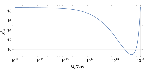
The model fits the data best when $M_{2}=4.50\times 10^{15}$ GeV, with $\chi^{2}=8.93$. The values of the free parameters and the predicted observables for the best-fit point are listed in Tab.3.

$M_{1}/$GeV	$M_{2}/$GeV	$a$	$b$	$\beta$	$n$
$5.140\times 10^{10}$	$4.500\times 10^{15}$	$0.008617$	$0.8834$	$2\pi/3$	3
$m_{2}$	$m_{3}$	$\theta_{12}$	$\theta_{13}$	$\theta_{23}$	$\delta$	$Y_{B}$	$\chi^{2}$
$8.70$ meV	$49.98$ meV	$33.89\degree$	$8.47\degree$	$44.3\degree$	$266\degree$	$8.72\times 10^{-11}$	$8.93$

Table 3: Best-fit point found by a three-dimensional random walk with random step size in ${a,\,b,\,M_{1}}$ for different values of $M_{2}$. We have fitted the results assuming the NuFit data with SK atmospheric data.

Among the observables, $\theta_{23}$ shows the greatest deviation from the NuFit result, being outside the $1\sigma$ range. However, the global fit result of $\theta_{23}$ is non-Gaussian. For individual experiments, the combination of ${\theta_{23},\,\delta}$ still lies in the $1\sigma$ range allowed by the T2K result and $2\sigma$ range allowed by the NOvA result Esteban:2020cvm .

2.1.1 Neutrinoless double beta decay

The Majorana nature of neutrinos would lead to neutrinoless double beta decay ($0\nu\beta\beta$). The key parameter affecting the decay rate (or the half-life time) of nucleons due to the mediation of light Majorana neutrinos is described by the effective mass $m_{\beta\beta}$, which is determined by the mass spectrum and PMNS mixing matrix. In the framework of the Littlest Seesaw model, the neutrino mass spectrum and mixing matrix are completely fixed by the neutrino data. Following the curve in Fig.1, the model predicts $m_{\beta\beta}$ around 4 meV, beyond the sensitivity of the next generation experiments nEXO:2021ujk ; LEGEND:2021bnm , which is consistent with the common result in the normal ordering case with the lightest neutrino massless Giuliani:2019uno .

2.1.2 Vacuum stability

As the couplings run from low scale to high scale, the Higgs quartic coupling can become negative, leading to breaking of the stability of the vacuum. Within SM, the RG equation of the Higgs quartic coupling at 1-loop level is given by Degrassi:2012ry

$$(4\pi)^{2}\frac{d\lambda_{H}}{d\ln\mu} = \frac{3}{8}\left(g_{1}^{4}+2g_{1}^{2}g_{2}^{2}+3g_{2}^{4}\right)-6y_{t}^{4}+\left(12y_{t}^{2}-3g_{1}^{2}-9g_{2}^{2}\right)\lambda_{H}+24\lambda_{H}^{2}\,.$$ (13)

Such running depends significantly on the Yukawa coupling (or the mass) of the top quark since it the largest among other couplings. In the seesaw extension of SM, the seesaw Yukawa couplings contributes negatively to the RG equation Antusch:2005gp

$$(4\pi)^{2}\frac{d\lambda_{H}}{d\ln\mu} = \frac{3}{8}\left(g_{1}^{4}+2g_{1}^{2}g_{2}^{2}+3g_{2}^{4}\right)-6y_{t}^{4}-2\text{Tr}[Y_{\nu}^{\dagger}Y_{\nu}Y_{\nu}^{\dagger}Y_{\nu}]$$ (14)

$$\quad\quad+\left(12y_{t}^{2}+\text{Tr}[Y_{\nu}^{\dagger}Y_{\nu}]-3g_{1}^{2}-9g_{2}^{2}\right)\lambda_{H}+24\lambda_{H}^{2}\,.$$

For heavy RH neutrinos, the seesaw Yukawa coupling can be quite large (close to O(1)), leading to a sharp decrease to values below zero of the SM Higgs quartic coupling at scales above the mass of the heaviest RH neutrino Mandal:2019ndp . This makes the SM Higgs potential unbounded from below and makes the vacuum unstable. However, the existence of the new heavy scalar, which as similar mass to the heavy neutrinos, can also couple to the Higgs through $\lambda_{H\Phi}H^{2}\Phi^{2}$, providing an extra contribution to the RG equation. At 1-loop level, the RG equations are given by Elias-Miro:2012eoi

$$(4\pi)^{2}\frac{d\lambda_{H}}{d\ln\mu} = \frac{3}{8}\left(g_{1}^{4}+2g_{1}^{2}g_{2}^{2}+3g_{2}^{4}\right)-6y_{t}^{4}-2\text{Tr}[Y_{\nu}^{\dagger}Y_{\nu}Y_{\nu}^{\dagger}Y_{\nu}]$$

$$\quad\quad+\left(12y_{t}^{2}+\text{Tr}[Y_{\nu}^{\dagger}Y_{\nu}]-3g_{1}^{2}-9g_{2}^{2}\right)\lambda_{H}+24\lambda_{H}^{2}+4\lambda_{H\Phi}^{2}$$

$$(4\pi)^{2}\frac{d\lambda_{H\Phi}}{d\ln\mu} = \frac{1}{2}\left(g_{1}^{4}+2g_{1}^{2}g_{2}^{2}+3g_{2}^{4}\right)+8\lambda_{\Phi}^{2}+4(3\lambda_{H}+2\lambda_{\Phi})\lambda_{H\Phi}$$ (15)

$$(4\pi)^{2}\frac{d\lambda_{\Phi}}{d\ln\mu} = -\frac{1}{8}\sum_{i}y_{i}^{4}+8\lambda_{H\Phi}^{2}+\sum_{i}y_{i}^{2}\lambda_{\Phi}+20\lambda_{\Phi}^{2}$$

The negative contribution from the seesaw Yukawa can be compensated with the positive contribution from the coupling between SM Higgs and the heavy scalar $\lambda_{H\Phi}$, and one may avoid the vacuum instability Mandal:2019ndp .

3 Gravitational Waves from Global Cosmic Strings

Figure 2: Gravitational wave spectrum from a global cosmic string network with $U(1)_{\rm B-L}$ symmetry breaking scale $\eta=10^{14},10^{15}$ GeV.

Cosmic strings (CS) are topological defects that are produced due to $U(1)$ symmetry breaking in the early universe Hindmarsh:1994re ; Vilenkin:2000jqa ; Vachaspati:2015cma . These topological defects behave as dynamical classical objects moving at relativistic speed. In context to string theory however, the description of these objects are sometimes as fundamental or somtimes as composite objects Witten:1985fp ; Dvali:2003zj ; Copeland:2003bj ; Polchinski:2004ia ; Sakellariadou:2008ie ; Davis:2008dj ; Sakellariadou:2009ev ; Copeland:2009ga . Interestingly, CS networks once formed offer very promising sources of GW of cosmological origin which maybe detected in near future. Moreover several Standard Model extensions, such as models of Grand Unified Theory (GUT) Jeannerot:2003qv ; Sakellariadou:2007bv ; Buchmuller:2013lra , or the seesaw mechanism for generating the neutrino masses in the Standard Model when $U_{B-L}(1)$ is broken spontaneously Dror:2019syi .

The cosmic string network is characterized by its correlation length $L$. When the strings are stretched by cosmic expansion, they form loops. This would mean we may expect that $L$ evolves linearly with the scale factor $a$ due to the background Hubble expansion, in a manner that $L\propto t^{1/2}$ during radiation domination epoch and $L\propto t^{2/3}$ during the matter domination. But this turns out to be incorrect. From we find from the simulations of cosmic strings is that the system reaches its scaling regime after a transient evolution. During this period the energy loss of long strings into loop formation, is exactly the same as that as if $L$ scales linearly with the Hubble horizon $t$ Ringeval:2005kr ; Vanchurin:2005pa ; Martins:2005es ; Olum:2006ix ; BlancoPillado:2011dq . Therefore, the CS evolutionary dynamics during this regime is only characterized by the string tension $\mu$, which is approximately equal to the phase transition temperature $T_{p}$ squared given as

$$G\mu\simeq 10^{-15}\left(\frac{T_{p}}{10^{11}~{}\text{GeV}}\right)^{2}.$$ (16)

The long string energy density, $\rho_{\infty}=\mu/L^{2}$ redshifts as radiation in radiation domination and as matter in matter domination epochs in early universe in the scaling regime.

The oscillations of the CS loops are known to be large dominant source of the Stochastic Gravitational Waves Background (SGWB). These long-standing source starts to emit GW after the network formation and still radiating today Vilenkin:1981bx ; Hogan:1984is ; Vachaspati:1984gt ; Accetta:1988bg ; Bennett:1990ry ; Caldwell:1991jj ; Allen:1991bk ; Battye:1997ji ; DePies:2007bm ; Siemens:2006yp ; Olmez:2010bi ; Regimbau:2011bm ; Sanidas:2012ee ; Sanidas:2012tf ; Binetruy:2012ze ; Kuroyanagi:2012wm ; Kuroyanagi:2012jf . The prediction of the SGWB from CS is that these GW consists of frequencies spanning over many orders of magnitude in frequency. Hence, the capability of the next generation of GW interferometers, LISA Audley:2017drz , Einstein Telescope Hild:2010id ; Punturo:2010zz , Cosmic Explorer Evans:2016mbw , BBO and DECIGO Yagi:2011wg to detect the SGWB from CS. This naturally gives us a unique observational window, on any new physics beyond the SM in early universe like we allude to, in the littlest seesaw model. For our analysis, we will refer to Ref. Kibble:1976sj for the original article, Ref. Vilenkin:2000jqa for a textbook, and Refs. Gouttenoire:2019kij ; Auclair:2019wcv ; Gouttenoire:2022gwi ; Ghoshal:2023sfa for reviews of their spectrum arising due to the GW emission.

3.1 Short review for Global Cosmic Strings

The CS core has the size which is inverse of the scale of symmetry-breaking, typically much smaller than the cosmological horizon. Due to this it can be described as infinitely thin classical objects with energy per unit length also knwon as the $\mu$ (Nambu-Goto approximation) for the global cosmic strings,

$$\mu=2\pi n\,\eta^{2}\times\log(\eta t)$$ (17)

where $\eta$ represents the vacuum expectation value of the scalar field constituting CS, and $n$ is the winding number (taken to be $n=1$). Usually for global strings, the logarithmic divergence arises due to the presence of massless Goldstone mode. This means the existence of long-range gradient energy Vilenkin:2000jqa . As the CS network is formed below the temperature of the $U(1)$-breaking phase transition, the cosmic string tension is approximately given by

$$T_{\textrm{form}} \simeq\eta.$$ (18)

There exists no GW before the cosmic strings network is formed. The typical GW spectrum from global cosmic strings has a natural cut-off, which corresponds to the network formation giving us the frequency,

$$f_{\textrm{form}}~{}\simeq{1\rm GHz}\times 0.47\left(\frac{T_{\rm form}}{10^{14}~{}{\rm GeV}}\right)\left(\frac{0.1}{\alpha}\right)\left[\frac{g_{*}(T_{\rm form})}{g_{*}(T_{0})}\right]^{\frac{1}{4}},$$ (19)

where it has always assumed that the early universe is always radiation-dominated universe. This cut-off remains only in the ultra-high frequency regime, and is not probe-able by the future-planned GW interferometer-based GW detectors.

In general, the evolution of cosmic strings is initially frozen due to the presence of thermal friction; however afterwards it reaches an attractor solution called the scaling regime. It is during this period that the correlation length of the string network suffers linear growth with respect to the cosmic time, $L\propto t$ Vilenkin:2000jqa ; Martins:2000cs ; Martins:2016ois . Dedicated numerical simulations of cosmic strings Blanco-Pillado:2013qja show that the GW spectrum is dominantly produced via loops with the largest size, typically corresponding to $10\%$ of the Hubble horizon size. Although the loop may have some disctribution but the fact that even the largest cosmic string loop size is so very small compared to the Hubble means that we may take the loop size distribution to be monochromatic in nature for all practical purposes

$$P_{\alpha}(\alpha)=\delta(\alpha-0.1).$$ (20)

After their formation, loops oscillate and radiate GW at a frequency $\tilde{f}=2k/l$, where $l$ is the loop length and $k\in\mathbb{Z}^{+}$ denotes the usual Fourier mode index under consideration. The frequency of the GW observed today is given by $f=\tilde{f}[a(\tilde{t})/a(t_{0})].$ where the subscript 0 represents present time. Each Fourier mode $k$ radiates GW with power

$$P_{\rm GW}^{(k)}=\Gamma^{(k)}G\mu^{2},\qquad\text{with}\quad\Gamma^{(m)}=\frac{\Gamma k^{-{\delta}}}{\sum_{p=1}^{\infty}p^{-\delta}},$$ (21)

where $\Gamma=50$ Blanco-Pillado:2017oxo . The index $\delta$ depends on whether high Fourier modes are dominated by cusps ($\delta=4/3$), kinks ($\delta=5/3$), and kink-kink collision $(\delta=2)$ Olmez:2010bi . The strings will lose energy incessantly leading to shrinking of the loop length $l$

$$l(\tilde{t})=\alpha t_{i}-(\Gamma G\mu+\kappa)(\tilde{t}-t_{i}).$$ (22)

where $\Gamma G\mu$ and $\kappa$ represent the shrinking rates due to GW and particle emissions, respectively.

Written from right to left, are in chronological order the various processes that occur and lead us to the final expression for the spectral energy density of GWs from CS, defined as $\Omega_{\rm GW}\equiv\frac{1}{\rho_{c}}\frac{d\rho_{\rm GW}}{d\ln{f}}$,

$$\Omega_{\rm GW}(f) =\sum_{m}\frac{1}{\rho_{c}}\int_{t_{\rm osc}}^{t_{0}}d\tilde{t}\int_{0}^{1}d\alpha\,\Theta\left[t_{i}-\frac{l_{*}}{\alpha}\right]\cdot\Theta[t_{i}-t_{\rm osc}]\cdot\left[\frac{a(\tilde{t})}{a(t_{0})}\right]^{4}\cdot P_{\rm GW}^{(m)}\times$$

$$\hskip 150.00023pt\times\left[\frac{a(t_{i})}{a(\tilde{t})}\right]^{3}\cdot P_{\alpha}(\alpha)\cdot\frac{dt_{i}}{df}\cdot\frac{dn_{\rm loop}}{dt_{i}}.$$ (23)

which simplifies to Gouttenoire:2019kij

$$\Omega_{\rm std}^{\rm CS}h^{2} \simeq\Omega_{r}h^{2}\,\Delta_{\rm R}\,C_{\rm eff}^{\rm rad}\cdot 9\left[\frac{\Gamma}{\Gamma_{\rm gold}}\right]\left[\frac{\eta}{M_{\rm Pl}}\right]^{4}\log^{3}\left[\eta\tilde{t}_{\rm M}\right],$$ (24)

$$\simeq 1.2\cdot 10^{-17}\left[\frac{\eta}{10^{15}~{}{\rm GeV}}\right]^{4}\log^{3}\left\{5.6\cdot 10^{30}\left[\frac{\eta}{10^{15}~{}{\rm GeV}}\right]\left[\frac{1~{}{\rm mHz}}{f}\right]^{\!2}\right\},$$ (25)

where $\Omega_{r}h^{2}\simeq 4.2\times 10^{-5}$ ParticleDataGroup:2020ssz is the radiation density today, and $\Delta_{\rm R}$ gives the information on the change in Universe expansion rate due to the change of the number of relativistic species,

$$\Delta_{\rm R}(T)\equiv\left(\frac{g_{*}(T)}{g_{*}(T_{0})}\right)\left(\frac{g_{*}s(T_{0})}{g_{*s}(T)}\right)^{4/3}=~{}0.39\left(\frac{106.75}{g_{*}(T)}\right)^{1/3}.$$ (26)

3.2 Existing constraints on Global strings

Massless Goldstone particles can be produced efficiently by global cosmic strings, contributing to the number $N_{\rm eff}$ of effective relativistic degrees of freedom. The precise constraint depends on how many Goldstone particles can be produced from strings, which is still debatable. Very recent studies Hindmarsh:2019csc ; Hindmarsh:2021vih ; Buschmann:2019icd ; Buschmann:2021sdq claim that the Goldstone energy spectrum from strings is scale-invariant, while other also recent studies Gorghetto:2018myk ; Gorghetto:2020qws ; Gorghetto:2021fsn suggest a slightly infrared-dominated spectrum, which leads to the production of more Goldstone particles. Here we quote the upper bound $\eta\lesssim 3.5\cdot 10^{15}\,{\rm GeV}$ derived in Ref. Chang:2021afa and refer to Refs. Gorghetto:2021fsn ; Dror:2021nyr for slightly tighter bounds.

The measurements of CMB show no evidence of B-mode polarization. This gives us yet another constraint on the global cosmic string network. If one assumes instantaneous reheating and the presence of only the SM degrees of freedom, the upper bound on the primordial inflationary Hubble parameter $H_{\rm inf}\lesssim 3\times 10^{13}~{}\rm GeV$ BICEP:2021xfz roughly gives the estimate for the maximum possible temperature of the universe to be $T_{\rm max}\lesssim 4\times 10^{15}$ GeV. Therefore, for the string network to form, the string scale $\eta$ must be at least smaller than the maximum temperature $\eta\lesssim 4\times 10^{15}$ GeV, up to $\mathcal{O}(1)$ model-dependent parameters.

Additional constraints arise due to the potential distortion of the CMB power spectrum by global cosmic strings Planck:2015fie ; Charnock:2016nzm ; Lopez-Eiguren:2017dmc . For $\eta\gtrsim 10^{15}\,{\rm GeV}$, GW from global strings extend to $f\lesssim 10^{-14}\,{\rm Hz}$. This in principle leaves its signature in CMB polarization experiments, e.g. Ref. BICEP:2021xfz . However, the GW in this frequency range can only be produced after photon decoupling, evading the CMB constraint. We refer the reader to see Fig. 8 of Ref. Chang:2021afa .

3.3 GW Detectors

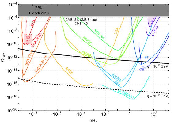
In Fig.2, we display the expected sensitivity reaches for various current and planned GW experiments which can be categorized as following:

• ground based interferometers: LIGO/VIRGO LIGOScientific:2016aoc ; LIGOScientific:2016sjg ; LIGOScientific:2017bnn ; LIGOScientific:2017vox ; LIGOScientific:2017ycc ; LIGOScientific:2017vwq , aLIGO/aVIRGO LIGOScientific:2014pky ; VIRGO:2014yos ; LIGOScientific:2019lzm , AION Badurina:2021rgt ; Graham:2016plp ; Graham:2017pmn ; Badurina:2019hst , Einstein Telescope (ET) Punturo:2010zz ; Hild:2010id , Cosmic Explorer (CE) LIGOScientific:2016wof ; Reitze:2019iox ,

• space based interferometers: LISA LISA:2017pwj ; Baker:2019nia , BBO Crowder:2005nr ; Corbin:2005ny , DECIGO, U-DECIGOSeto:2001qf ; Kudoh:2005as ; Nakayama:2009ce ; Yagi:2011wg ; Kawamura:2020pcg , AEDGE AEDGE:2019nxb ; Badurina:2021rgt , $\mu$-ARES Sesana:2019vho

• CMB spectral distortions: PIXIE, Super-PIXIE Kogut:2019vqh , VOYAGER2050 Chluba:2019kpb

• recasts of star surveys: GAIA/THEIA Garcia-Bellido:2021zgu ,

• CMB polarization: Planck 2018 Akrami:2018odb and BICEP 2/ Keck BICEP2:2018kqh computed by Clarke:2020bil , LiteBIRD Hazumi:2019lys ,

• pulsar timing arrays (PTA): Square-Kilometer-Array (SKA) Carilli:2004nx ; Janssen:2014dka ; Weltman:2018zrl , EPTA Lentati:2015qwp ; Babak:2015lua , NANOGRAV McLaughlin:2013ira ; NANOGRAV:2018hou ; Aggarwal:2018mgp ; Brazier:2019mmu ; NANOGrav:2020bcs

3.4 Dark radiation bounds from BBN and CMB decoupling

At last the energy density of the primordial gravitational waves should be smaller than the limit on dark radiation encoded in $\Delta N_{\text{eff.}}$ from Big Bang Nucleosynthesis and CMB observations (see the discussion in the text for bounds and projections on $\Delta N_{\text{eff.}}$). The change of the number of effective relativistic degrees of freedom (Neff ) at recombination time is given by an amount Maggiore:1999vm

$$\int_{f_{\text{min}}}^{f=\infty}\frac{\text{d}f}{f}\Omega_{\text{GW}}(f)h^{2}\leq 5.6\times 10^{-6}\;\Delta N_{\text{eff.}}.$$ (27)

The lower limit for the integration is taken to be $f_{\text{min}}\simeq 10^{-10}\text{Hz}$ for BBN and $f_{\text{min}}\simeq 10^{-18}\text{Hz}$ for the CMB bounds. However we may approximately ignore the frequency dependence to constrain the energy density of the peak for a given GW spectrum to be

$$\Omega_{\text{GW}}^{\text{Peak}}h^{2}\leq 5.6\times 10^{-6}\;\Delta N_{\text{eff.}}.$$ (28)

4 Gravitational wave from $U(1)_{B-L}$ symmetry breaking

As having been discussed in Sec.2, the scale of $U(1)_{B-L}$ symmetry breaking can be related to the masses of RH neutrinos through a single group of Yukawa couplings, namely the $y_{i}$ in Eq.2. On the other hand, GW detectors can detect the gravitational waves produced by the cosmic strings resulting from the $U(1)_{B-L}$ symmetry breaking, whose strength is dominantly determined by the scale of $U(1)$ symmetry breaking. As a consequence, it is possible to constraint the masses of RH neutrinos through gravitational wave detection, up to the Yukawa coupling $y_{i}$. In particular, if a certain upper bound of the Higgs singlet VEV is obtained from gravitational wave observation, the heaviest RH neutrino, which has the largest Yukawa coupling to the heavy Higgs singlet, cannot be much heavier than that upper bound due to the perturbativity limit of the coupling.

In Fig.3, we show how this kind of connection between RH neutrino mass and the GW observations works. The heaviest RHN mass is labelled as $M$ and the corresponding coupling to the Higgs singlet is $y$. The colour filled in the figure stands for the value of $y$. Below the black solid line, the white region is where the coupling is larger than its perturbativity limit and thus not considered theoretically. The constraints on the VEV of the Higgs singlet are shown are the shadowed areas and the sensitivities of GW detectors are shown as the horizontal lines. In particular, if any of the GW detectors does not find any signal, the region above the corresponding line would be excluded. Combined the perturbativity limit, the GW detection can be used to test models with the heaviest RH neutrino mass above $2.5\times 10^{14}$ GeV.

Figure 3: Constraints and sensitivities in the $M-\eta$ plane. The various GW detectors shown here tell us the range of $U(1)_{\rm B-L}$ symmetry breaking scales that it will be able to probe via the measurements of the GW spectrum. The horizontal scale represents the heaviest RH neutrino mass, and the lines and contours show the Yukawa coupling of this neutrino to the $B-L$ breaking scalar, whose VEV is indicated by the LH vertical axis. The pink band is the favoured heavier RH neutrino mass in the Littlest Seesaw model, which can be fully probed by future GW experiments. See the text for further details.

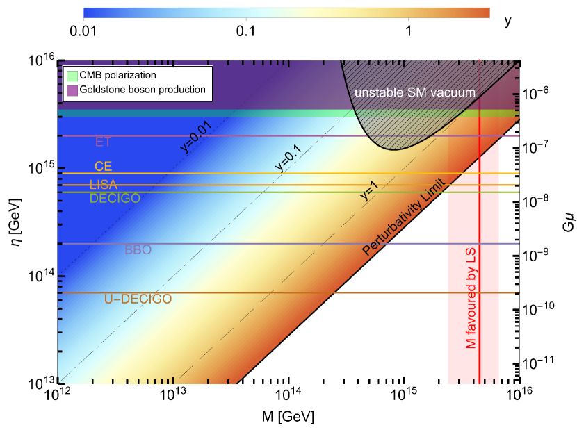
As an example, the case of the Littlest Seesaw model fitting to the NuFit result with SK atmospheric data is presented in Fig.3. The red vertical line marks the value of the heaviest RH neutrino mass in the Littlest Seesaw model for the best-fit benchmark point in Tab.3. The region shadowed with red represents the allowed range of the heaviest RH neutrino mass requiring $\chi^{2}<10$. As can be read from the figure, the region where the Littlest Seesaw model can fit the neutrino data with $\chi^{2}<10$ can be excluded if no GW signal is observed by ET, CE and LISA. Further more, if all of the GW detectors in the figure cannot find and signal, the Littlest Seesaw model would be excluded at $\chi^{2}<16.0$ level. If the coupling $y$ is further required to be smaller than 1, the exclusion would be improved to $\chi^{2}<17.6$.

On the other hand, the GW detection in Fig.3 can be alternatively understood as constraints on the coupling $y$. For the best-fitted value of $M_{2}$ in the Littlest Seesaw model (the red line), ET can imply the coupling $y$ if it is below 5. In another word, if ET does not find any signal, the region where $y<5$ will be ruled out for the best-fitted point in the Littlest Seesaw model. If a model predicts a lower mass of the heaviest RH neutrino, then its coupling to the superheavy scalar field can be implied or constrained by more GW detection. For example, the coupling $y$ in a model predicting a $7\times 10^{13}$ GeV heaviest RH neutrino would be implied by U-DECIGO as long as it is smaller than 1.

As the right-handed neutrino mass becomes larger, the Yukawa coupling can be large enough to dominate over the top quark Yukawa coupling in the RG running of the Higgs quartic coupling 14. As a result, the SM vacuum can become unstable at high energies. In Fig.3, we identify the region where the SM vacuum stability breaks below the scale of the heavy scalar $\eta$ since the heavy scalar is integrated out of the theory. Above the scale of the heavy scalar, the coupling between $\Phi$ and Higgs boson can help preserving the stability of the SM vacuum.

5 Conclusion

The type I seesaw model not only accounts for the small neutrino masses and large mixing of the PMNS matrix elegantly but also provides a potential explanation of the matter-antimatter asymmetry via thermal leptogenesis. However, in the standard leptogenesis scenario, the lightest RH neutrino is typically above $10^{9}$ GeV, which is far beyond the accessibility of collider or astrophysical experiments.

In this paper, we have explored the possibility of constraining the RH neutrino mass with primordial gravitational wave detection. In the minimal natural extension of the type I seesaw models with a global $U(1)_{B-L}$ symmetry, the VEV of a superheavy scalar field, from which the RH neutrinos obtain their Majorana mass, breaks the $U(1)_{B-L}$ symmetry. During the corresponding phase transition in the early universe, global cosmic strings can be produced due to the $U(1)_{B-L}$ symmetry breaking. The dynamical evolution of the strings results in detectable GWs, whose amplitude can be determined by the symmetry breaking scale. As a result, the detection of GWs can be used to constrain the masses of heaviest RH neutrinos associated with the ${B-L}$ breaking.

In some models the RH neutrino masses are determined, leading to a decisive test of these models using GWs. As a concrete example, we have studied the Littlest Seesaw model, where only two RH neutrinos play a role in the seesaw mechanism and the Yukawa couplings in the flavour basis follow special alignments as required by discrete flavour symmetry. By fitting the model to neutrino data and baryon asymmetry, all of the free parameters in the model can be determined including the heavier RH neutrino mass, which is related to the $B-L$ breaking scale up to an arbitary Yukawa coupling. We have found that, due to the perturbativity limit of this coupling, the parameter space favoured by the Littlest Seesaw model can be fully probed by the proposed GW detectors including LISA, CE and ET. If no GW signal is found by these detectors, the entire parameter space of this model would be disfavoured. For more general type I seesaw models with a global $B-L$ symmetry, the above GW detectors can serve to constrain the coupling between the heaviest RH neutrino and the $B-L$ breaking scalar.

In summary, gravitational wave detection allows us to probe the heaviest RH neutrino mass in a general class of type I seesaw models with a global $U(1)_{B-L}$ symmetry. To illustrate this, we have analysed a specific example of a highly predictive type I seesaw model with two RH neutrinos and shown that it will be tested very soon by proposed gravitational wave detectors. The methodology can be extended to other type I seesaw models with a global $U(1)_{B-L}$ symmetry.

In future, it would be interesting to understand how such $U(1)$ global symmetries when embedded in UV-complete scenarios like SO(10) may lead to associated formation of other topological defects like domain walls and local cosmic strings or hybrid defect scenarios which may have their own unique GW signal corresponding to breaking pattern in the early universe like studied in Ref. Barman:2022yos ; Dunsky:2021tih or involving mixed GW signals from phase transitions and topological defects in standard and non-standard cosmological histories Ferrer:2023uwz ; Ghoshal:2023sfa .

We envisage that the precision measurements that the GW cosmology and GW astronomy aspire to reach from the planned global network of GW detectors will make the dream of testing high-scale physics and fundamental BSM scenarios of UV-completion a reality in the very near future.

Appendix A Appendix: Signal-to-noise ratio (SNR)

Gravitational Wave Interferometers actually measure displacements of detector arms in terms of a what is known in terms of dimensionless strain-noise $h_{\text{GW}}(f)$ which is related to the GW amplitude. This can be straight-forwardly converted into the corresponding energy density Garcia-Bellido:2021zgu

$$\Omega_{\text{exp}}(f)h^{2}=\frac{2\pi^{2}f^{2}}{3H_{0}^{2}}h_{\text{GW}}(f)^{2}h^{2},$$ (29)

where $H_{0}=h\times 100\;\text{(km/s)}/\text{Mpc}$ is the Hubble expansion rate today. The signal-to-noise ratio (SNR) for a projected experimental sensitivity $\Omega_{\text{exp}}(f)h^{2}$ is then estimated in order to assess the detection probability of the primordial GW background originating from the global cosmic string background following the prescription Thrane:2013oya ; Caprini:2015zlo

$$\text{SNR}\equiv\sqrt{\tau\int_{f_{\text{min}}}^{f_{\text{max}}}\text{d}f\left(\frac{\Omega_{\text{GW}}(f)h^{2}}{\Omega_{\text{exp}}(f)h^{2}}\right)^{2}},$$ (30)

where $h=0.7$ and $\tau=4\;\text{years}$ is the observation time. Usually this is chosen to be $\text{SNR}\geq 10$ as the detection threshold for each individual detector.

References

- (1) T. Ohlsson, Special Issue on “Neutrino Oscillations: Celebrating the Nobel Prize in Physics 2015” in Nuclear Physics B, Nuclear Physics B 908 (2016) 1.
- (2) S. Weinberg, Baryon and Lepton Nonconserving Processes, Phys. Rev. Lett. 43 (1979) 1566.
- (3) P. Minkowski, at a Rate of One Out of Muon Decays?, Phys. Lett. B 67 (1977) 421.
- (4) T. Yanagida, Horizontal gauge symmetry and masses of neutrinos, Conf. Proc. C 7902131 (1979) 95.
- (5) M. Gell-Mann, P. Ramond and R. Slansky, Complex Spinors and Unified Theories, Conf. Proc. C 790927 (1979) 315 [1306.4669].
- (6) R.N. Mohapatra and G. Senjanovic, Neutrino Mass and Spontaneous Parity Nonconservation, Phys. Rev. Lett. 44 (1980) 912.
- (7) M. Magg and C. Wetterich, Neutrino Mass Problem and Gauge Hierarchy, Phys. Lett. B 94 (1980) 61.
- (8) J. Schechter and J.W.F. Valle, Neutrino Masses in SU(2) x U(1) Theories, Phys. Rev. D 22 (1980) 2227.
- (9) C. Wetterich, Neutrino Masses and the Scale of B-L Violation, Nucl. Phys. B 187 (1981) 343.
- (10) G. Lazarides, Q. Shafi and C. Wetterich, Proton Lifetime and Fermion Masses in an SO(10) Model, Nucl. Phys. B 181 (1981) 287.
- (11) R.N. Mohapatra and G. Senjanovic, Neutrino Masses and Mixings in Gauge Models with Spontaneous Parity Violation, Phys. Rev. D 23 (1981) 165.
- (12) E. Ma and U. Sarkar, Neutrino masses and leptogenesis with heavy Higgs triplets, Phys. Rev. Lett. 80 (1998) 5716 [hep-ph/9802445].
- (13) R. Foot, H. Lew, X.G. He and G.C. Joshi, Seesaw Neutrino Masses Induced by a Triplet of Leptons, Z. Phys. C 44 (1989) 441.
- (14) E. Ma, Pathways to naturally small neutrino masses, Phys. Rev. Lett. 81 (1998) 1171 [hep-ph/9805219].
- (15) E. Ma and D.P. Roy, Heavy triplet leptons and new gauge boson, Nucl. Phys. B 644 (2002) 290 [hep-ph/0206150].
- (16) T. Hambye, Y. Lin, A. Notari, M. Papucci and A. Strumia, Constraints on neutrino masses from leptogenesis models, Nucl. Phys. B 695 (2004) 169 [hep-ph/0312203].
- (17) S.F. King, Large mixing angle MSW and atmospheric neutrinos from single right-handed neutrino dominance and U(1) family symmetry, Nucl. Phys. B 576 (2000) 85 [hep-ph/9912492].
- (18) S.F. King, Constructing the large mixing angle MNS matrix in seesaw models with right-handed neutrino dominance, JHEP 09 (2002) 011 [hep-ph/0204360].
- (19) P.H. Frampton, S.L. Glashow and T. Yanagida, Cosmological sign of neutrino CP violation, Phys. Lett. B 548 (2002) 119 [hep-ph/0208157].
- (20) M. Fukugita and T. Yanagida, Baryogenesis Without Grand Unification, Phys. Lett. B 174 (1986) 45.
- (21) W.-l. Guo and Z.-z. Xing, Calculable CP violating phases in the minimal seesaw model of leptogenesis and neutrino mixing, Phys. Lett. B 583 (2004) 163 [hep-ph/0310326].
- (22) A. Ibarra and G.G. Ross, Neutrino phenomenology: The Case of two right-handed neutrinos, Phys. Lett. B 591 (2004) 285 [hep-ph/0312138].
- (23) J.-w. Mei and Z.-z. Xing, Radiative corrections to neutrino mixing and CP violation in the minimal seesaw model with leptogenesis, Phys. Rev. D 69 (2004) 073003 [hep-ph/0312167].
- (24) W.-l. Guo, Z.-z. Xing and S. Zhou, Neutrino Masses, Lepton Flavor Mixing and Leptogenesis in the Minimal Seesaw Model, Int. J. Mod. Phys. E 16 (2007) 1 [hep-ph/0612033].
- (25) S. Antusch, P. Di Bari, D.A. Jones and S.F. King, Leptogenesis in the Two Right-Handed Neutrino Model Revisited, Phys. Rev. D 86 (2012) 023516 [1107.6002].
- (26) K. Harigaya, M. Ibe and T.T. Yanagida, Seesaw Mechanism with Occam’s Razor, Phys. Rev. D 86 (2012) 013002 [1205.2198].
- (27) J. Zhang and S. Zhou, A Further Study of the Frampton-Glashow-Yanagida Model for Neutrino Masses, Flavor Mixing and Baryon Number Asymmetry, JHEP 09 (2015) 065 [1505.04858].
- (28) S.F. King, Minimal predictive see-saw model with normal neutrino mass hierarchy, JHEP 07 (2013) 137 [1304.6264].
- (29) F. Björkeroth and S.F. King, Testing constrained sequential dominance models of neutrinos, J. Phys. G 42 (2015) 125002 [1412.6996].
- (30) S.F. King, Littlest Seesaw, JHEP 02 (2016) 085 [1512.07531].
- (31) F. Björkeroth, F.J. de Anda, I. de Medeiros Varzielas and S.F. King, Towards a complete A SU(5) SUSY GUT, JHEP 06 (2015) 141 [1503.03306].
- (32) F. Björkeroth, F.J. de Anda, I. de Medeiros Varzielas and S.F. King, Leptogenesis in minimal predictive seesaw models, JHEP 10 (2015) 104 [1505.05504].
- (33) S.F. King and C. Luhn, Littlest Seesaw model from S U(1), JHEP 09 (2016) 023 [1607.05276].
- (34) P. Ballett, S.F. King, S. Pascoli, N.W. Prouse and T. Wang, Precision neutrino experiments vs the Littlest Seesaw, JHEP 03 (2017) 110 [1612.01999].
- (35) S.F. King, S. Molina Sedgwick and S.J. Rowley, Fitting high-energy Littlest Seesaw parameters using low-energy neutrino data and leptogenesis, JHEP 10 (2018) 184 [1808.01005].
- (36) M. Chianese, B. Fu and S.F. King, Minimal Seesaw extension for Neutrino Mass and Mixing, Leptogenesis and Dark Matter: FIMPzillas through the Right-Handed Neutrino Portal, JCAP 03 (2020) 030 [1910.12916].
- (37) M. Chianese, B. Fu and S.F. King, Interplay between neutrino and gravity portals for FIMP dark matter, JCAP 01 (2021) 034 [2009.01847].
- (38) LIGO Scientific, Virgo, 1M2H, Dark Energy Camera GW-E, DES, DLT40, Las Cumbres Observatory, VINROUGE, MASTER collaboration, A gravitational-wave standard siren measurement of the Hubble constant, Nature 551 (2017) 85 [1710.05835].
- (39) LISA collaboration, Laser Interferometer Space Antenna, 1702.00786.
- (40) K. Yagi and N. Seto, Detector configuration of DECIGO/BBO and identification of cosmological neutron-star binaries, Phys. Rev. D 83 (2011) 044011 [1101.3940].
- (41) M. Punturo et al., The Einstein Telescope: A third-generation gravitational wave observatory, Class. Quant. Grav. 27 (2010) 194002.
- (42) S. Hild et al., Sensitivity Studies for Third-Generation Gravitational Wave Observatories, Class. Quant. Grav. 28 (2011) 094013 [1012.0908].
- (43) LIGO Scientific collaboration, Exploring the Sensitivity of Next Generation Gravitational Wave Detectors, Class. Quant. Grav. 34 (2017) 044001 [1607.08697].
- (44) J.A. Dror, T. Hiramatsu, K. Kohri, H. Murayama and G. White, Testing the Seesaw Mechanism and Leptogenesis with Gravitational Waves, Phys. Rev. Lett. 124 (2020) 041804 [1908.03227].
- (45) B. Barman, D. Borah, A. Dasgupta and A. Ghoshal, Probing high scale Dirac leptogenesis via gravitational waves from domain walls, Phys. Rev. D 106 (2022) 015007 [2205.03422].
- (46) D.I. Dunsky, A. Ghoshal, H. Murayama, Y. Sakakihara and G. White, GUTs, hybrid topological defects, and gravitational waves, Phys. Rev. D 106 (2022) 075030 [2111.08750].
- (47) A. Dasgupta, P.S.B. Dev, A. Ghoshal and A. Mazumdar, Gravitational wave pathway to testable leptogenesis, Phys. Rev. D 106 (2022) 075027 [2206.07032].
- (48) D. Borah, A. Dasgupta and I. Saha, Leptogenesis and dark matter through relativistic bubble walls with observable gravitational waves, JHEP 11 (2022) 136 [2207.14226].
- (49) B. Fu and S.F. King, Gravitational wave signals from leptoquark-induced first-order electroweak phase transitions, JCAP 05 (2023) 055 [2209.14605].
- (50) D. Borah, A. Dasgupta and I. Saha, LIGO-VIRGO constraints on dark matter and leptogenesis triggered by a first order phase transition at high scale, 2304.08888.
- (51) A. Ghoshal, R. Samanta and G. White, Bremsstrahlung High-frequency Gravitational Wave Signatures of High-scale Non-thermal Leptogenesis, 2211.10433.
- (52) N. Bhaumik, A. Ghoshal and M. Lewicki, Doubly peaked induced stochastic gravitational wave background: testing baryogenesis from primordial black holes, JHEP 07 (2022) 130 [2205.06260].
- (53) N. Bhaumik, A. Ghoshal, R.K. Jain and M. Lewicki, Distinct signatures of spinning PBH domination and evaporation: doubly peaked gravitational waves, dark relics and CMB complementarity, 2212.00775.
- (54) D. Borah, S. Jyoti Das and R. Roshan, Probing high scale seesaw and PBH generated dark matter via gravitational waves with multiple tilts, 2208.04965.
- (55) T. Vachaspati and A. Vilenkin, Gravitational Radiation from Cosmic Strings, Phys. Rev. D 31 (1985) 3052.
- (56) W. Buchmüller, V. Domcke, K. Kamada and K. Schmitz, The Gravitational Wave Spectrum from Cosmological Breaking, JCAP 10 (2013) 003 [1305.3392].
- (57) W. Chao, W.-F. Cui, H.-K. Guo and J. Shu, Gravitational wave imprint of new symmetry breaking, Chin. Phys. C 44 (2020) 123102 [1707.09759].
- (58) N. Okada and O. Seto, Probing the seesaw scale with gravitational waves, Phys. Rev. D 98 (2018) 063532 [1807.00336].
- (59) W. Buchmuller, V. Domcke, H. Murayama and K. Schmitz, Probing the scale of grand unification with gravitational waves, Phys. Lett. B 809 (2020) 135764 [1912.03695].
- (60) T. Hasegawa, N. Okada and O. Seto, Gravitational waves from the minimal gauged model, Phys. Rev. D 99 (2019) 095039 [1904.03020].
- (61) N. Haba and T. Yamada, Gravitational waves from phase transition in minimal SUSY model, Phys. Rev. D 101 (2020) 075027 [1911.01292].
- (62) S. Blasi, V. Brdar and K. Schmitz, Fingerprint of low-scale leptogenesis in the primordial gravitational-wave spectrum, Phys. Rev. Res. 2 (2020) 043321 [2004.02889].
- (63) F. Ferrer, A. Ghoshal and M. Lewicki, Imprints of a Supercooled Universe in the Gravitational Wave Spectrum from a Cosmic String network, 2304.02636.
- (64) P. Di Bari, S.F. King and M.H. Rahat, Gravitational waves from phase transitions and cosmic strings in neutrino mass models with multiple Majorons, 2306.04680.
- (65) F. Wilczek and A. Zee, Operator Analysis of Nucleon Decay, Phys. Rev. Lett. 43 (1979) 1571.
- (66) H.J. Lipkin, Why Is Conserved and Baryon Number Not in Unified Models of Quarks and Leptons?, Phys. Rev. Lett. 45 (1980) 311.
- (67) J. Heeck, Unbroken B – L symmetry, Phys. Lett. B 739 (2014) 256 [1408.6845].
- (68) R.E. Marshak, invariance, B-L symmetry and naturalness, AIP Conf. Proc. 72 (1981) 665.
- (69) R.N. Mohapatra and G. Senjanovic, Hydrogen - Anti-hydrogen Oscillations and Spontaneously Broken Global Symmetry, Phys. Rev. Lett. 49 (1982) 7.
- (70) R.N. Mohapatra and G. Senjanovic, Spontaneous Breaking of Global l Symmetry and Matter - Antimatter Oscillations in Grand Unified Theories, Phys. Rev. D 27 (1983) 254.
- (71) A. Davidson, as the fourth color within an model, Phys. Rev. D 20 (1979) 776.
- (72) R.N. Mohapatra and R.E. Marshak, Local B-L Symmetry of Electroweak Interactions, Majorana Neutrinos and Neutron Oscillations, Phys. Rev. Lett. 44 (1980) 1316.
- (73) W. Buchmuller, C. Greub and P. Minkowski, Neutrino masses, neutral vector bosons and the scale of B-L breaking, Phys. Lett. B 267 (1991) 395.
- (74) T. Fukuyama, A. Ilakovac, T. Kikuchi, S. Meljanac and N. Okada, SO(10) group theory for the unified model building, J. Math. Phys. 46 (2005) 033505 [hep-ph/0405300].
- (75) S.F. King, S. Pascoli, J. Turner and Y.-L. Zhou, Gravitational Waves and Proton Decay: Complementary Windows into Grand Unified Theories, Phys. Rev. Lett. 126 (2021) 021802 [2005.13549].
- (76) S.F. King, S. Pascoli, J. Turner and Y.-L. Zhou, Confronting SO(10) GUTs with proton decay and gravitational waves, JHEP 10 (2021) 225 [2106.15634].
- (77) B. Fu, S.F. King, L. Marsili, S. Pascoli, J. Turner and Y.-L. Zhou, A predictive and testable unified theory of fermion masses, mixing and leptogenesis, JHEP 11 (2022) 072 [2209.00021].
- (78) N. Okada, O. Seto and H. Uchida, Gravitational waves from breaking of an extra in grand unification, PTEP 2021 (2021) 033B01 [2006.01406].
- (79) I. Esteban, M.C. Gonzalez-Garcia, M. Maltoni, T. Schwetz and A. Zhou, The fate of hints: updated global analysis of three-flavor neutrino oscillations, JHEP 09 (2020) 178 [2007.14792].
- (80) “NuFIT website.” www.nu-fit.org.
- (81) Planck collaboration, Planck 2018 results. VI. Cosmological parameters, Astron. Astrophys. 641 (2020) A6 [1807.06209].
- (82) nEXO collaboration, nEXO: neutrinoless double beta decay search beyond 1028 year half-life sensitivity, J. Phys. G 49 (2022) 015104 [2106.16243].
- (83) LEGEND collaboration, The Large Enriched Germanium Experiment for Neutrinoless Decay: LEGEND-1000 Preconceptual Design Report, 2107.11462.
- (84) APPEC Committee collaboration, Double Beta Decay APPEC Committee Report, 1910.04688.
- (85) G. Degrassi, S. Di Vita, J. Elias-Miro, J.R. Espinosa, G.F. Giudice, G. Isidori et al., Higgs mass and vacuum stability in the Standard Model at NNLO, JHEP 08 (2012) 098 [1205.6497].
- (86) S. Antusch, J. Kersten, M. Lindner, M. Ratz and M.A. Schmidt, Running neutrino mass parameters in see-saw scenarios, JHEP 03 (2005) 024 [hep-ph/0501272].
- (87) S. Mandal, R. Srivastava and J.W.F. Valle, Consistency of the dynamical high-scale type-I seesaw mechanism, Phys. Rev. D 101 (2020) 115030 [1903.03631].
- (88) J. Elias-Miro, J.R. Espinosa, G.F. Giudice, H.M. Lee and A. Strumia, Stabilization of the Electroweak Vacuum by a Scalar Threshold Effect, JHEP 06 (2012) 031 [1203.0237].
- (89) M.B. Hindmarsh and T.W.B. Kibble, Cosmic strings, Rept. Prog. Phys. 58 (1995) 477 [hep-ph/9411342].
- (90) A. Vilenkin and E.P.S. Shellard, Cosmic Strings and Other Topological Defects, Cambridge University Press (7, 2000).
- (91) T. Vachaspati, L. Pogosian and D. Steer, Cosmic Strings, Scholarpedia 10 (2015) 31682 [1506.04039].
- (92) E. Witten, Cosmic Superstrings, Phys. Lett. B 153 (1985) 243.
- (93) G. Dvali and A. Vilenkin, Formation and evolution of cosmic D strings, JCAP 03 (2004) 010 [hep-th/0312007].
- (94) E.J. Copeland, R.C. Myers and J. Polchinski, Cosmic F and D strings, JHEP 06 (2004) 013 [hep-th/0312067].
- (95) J. Polchinski, Introduction to cosmic F- and D-strings, in NATO Advanced Study Institute and EC Summer School on String Theory: From Gauge Interactions to Cosmology, pp. 229–253, 12, 2004 [hep-th/0412244].
- (96) M. Sakellariadou, Cosmic Superstrings, Phil. Trans. Roy. Soc. Lond. A 366 (2008) 2881 [0802.3379].
- (97) A.-C. Davis, P. Brax and C. van de Bruck, Brane Inflation and Defect Formation, Phil. Trans. Roy. Soc. Lond. A 366 (2008) 2833 [0803.0424].
- (98) M. Sakellariadou, Cosmic Strings and Cosmic Superstrings, Nucl. Phys. B Proc. Suppl. 192-193 (2009) 68 [0902.0569].
- (99) E.J. Copeland and T.W.B. Kibble, Cosmic Strings and Superstrings, Proc. Roy. Soc. Lond. A 466 (2010) 623 [0911.1345].
- (100) R. Jeannerot, J. Rocher and M. Sakellariadou, How generic is cosmic string formation in SUSY GUTs, Phys. Rev. D 68 (2003) 103514 [hep-ph/0308134].
- (101) M. Sakellariadou, Production of Topological Defects at the End of Inflation, Lect. Notes Phys. 738 (2008) 359 [hep-th/0702003].
- (102) C. Ringeval, M. Sakellariadou and F. Bouchet, Cosmological evolution of cosmic string loops, JCAP 02 (2007) 023 [astro-ph/0511646].
- (103) V. Vanchurin, K.D. Olum and A. Vilenkin, Scaling of cosmic string loops, Phys. Rev. D 74 (2006) 063527 [gr-qc/0511159].
- (104) C.J.A.P. Martins and E.P.S. Shellard, Fractal properties and small-scale structure of cosmic string networks, Phys. Rev. D 73 (2006) 043515 [astro-ph/0511792].
- (105) K.D. Olum and V. Vanchurin, Cosmic string loops in the expanding Universe, Phys. Rev. D 75 (2007) 063521 [astro-ph/0610419].
- (106) J.J. Blanco-Pillado, K.D. Olum and B. Shlaer, Large parallel cosmic string simulations: New results on loop production, Phys. Rev. D 83 (2011) 083514 [1101.5173].
- (107) A. Vilenkin, Gravitational radiation from cosmic strings, Phys. Lett. B 107 (1981) 47.
- (108) C.J. Hogan and M.J. Rees, Gravitational interactions of cosmic strings, Nature 311 (1984) 109.
- (109) F.S. Accetta and L.M. Krauss, The stochastic gravitational wave spectrum resulting from cosmic string evolution, Nucl. Phys. B 319 (1989) 747.
- (110) D.P. Bennett and F.R. Bouchet, Constraints on the gravity wave background generated by cosmic strings, Phys. Rev. D 43 (1991) 2733.
- (111) R.R. Caldwell and B. Allen, Cosmological constraints on cosmic string gravitational radiation, Phys. Rev. D 45 (1992) 3447.
- (112) B. Allen and E.P.S. Shellard, Gravitational radiation from cosmic strings, Phys. Rev. D 45 (1992) 1898.
- (113) R.A. Battye, R.R. Caldwell and E.P.S. Shellard, Gravitational waves from cosmic strings, in Conference on Topological Defects and CMB, pp. 11–31, 6, 1997 [astro-ph/9706013].
- (114) M.R. DePies and C.J. Hogan, Stochastic Gravitational Wave Background from Light Cosmic Strings, Phys. Rev. D 75 (2007) 125006 [astro-ph/0702335].
- (115) X. Siemens, V. Mandic and J. Creighton, Gravitational wave stochastic background from cosmic (super)strings, Phys. Rev. Lett. 98 (2007) 111101 [astro-ph/0610920].
- (116) S. Olmez, V. Mandic and X. Siemens, Gravitational-Wave Stochastic Background from Kinks and Cusps on Cosmic Strings, Phys. Rev. D 81 (2010) 104028 [1004.0890].
- (117) T. Regimbau, S. Giampanis, X. Siemens and V. Mandic, The stochastic background from cosmic (super)strings: popcorn and (Gaussian) continuous regimes, Phys. Rev. D 85 (2012) 066001 [1111.6638].
- (118) S.A. Sanidas, R.A. Battye and B.W. Stappers, Constraints on cosmic string tension imposed by the limit on the stochastic gravitational wave background from the European Pulsar Timing Array, Phys. Rev. D 85 (2012) 122003 [1201.2419].
- (119) S.A. Sanidas, R.A. Battye and B.W. Stappers, Projected constraints on the cosmic (super)string tension with future gravitational wave detection experiments, Astrophys. J. 764 (2013) 108 [1211.5042].
- (120) P. Binetruy, A. Bohe, C. Caprini and J.-F. Dufaux, Cosmological Backgrounds of Gravitational Waves and eLISA/NGO: Phase Transitions, Cosmic Strings and Other Sources, JCAP 06 (2012) 027 [1201.0983].
- (121) S. Kuroyanagi, K. Miyamoto, T. Sekiguchi, K. Takahashi and J. Silk, Forecast constraints on cosmic string parameters from gravitational wave direct detection experiments, Phys. Rev. D 86 (2012) 023503 [1202.3032].
- (122) S. Kuroyanagi, K. Miyamoto, T. Sekiguchi, K. Takahashi and J. Silk, Forecast constraints on cosmic strings from future CMB, pulsar timing and gravitational wave direct detection experiments, Phys. Rev. D 87 (2013) 023522 [1210.2829].
- (123) T.W.B. Kibble, Topology of Cosmic Domains and Strings, J. Phys. A 9 (1976) 1387.
- (124) Y. Gouttenoire, G. Servant and P. Simakachorn, Beyond the Standard Models with Cosmic Strings, JCAP 07 (2020) 032 [1912.02569].
- (125) P. Auclair et al., Probing the gravitational wave background from cosmic strings with LISA, JCAP 04 (2020) 034 [1909.00819].
- (126) Y. Gouttenoire, Beyond the Standard Model Cocktail, Springer Theses, Springer, Cham (2022), 10.1007/978-3-031-11862-3, [2207.01633].
- (127) A. Ghoshal, Y. Gouttenoire, L. Heurtier and P. Simakachorn, Primordial Black Hole Archaeology with Gravitational Waves from Cosmic Strings, 2304.04793.
- (128) C.J.A.P. Martins and E.P.S. Shellard, Extending the velocity dependent one scale string evolution model, Phys. Rev. D 65 (2002) 043514 [hep-ph/0003298].
- (129) C.J.A.P. Martins, I.Y. Rybak, A. Avgoustidis and E.P.S. Shellard, Extending the velocity-dependent one-scale model for domain walls, Phys. Rev. D 93 (2016) 043534 [1602.01322].
- (130) J.J. Blanco-Pillado, K.D. Olum and B. Shlaer, The number of cosmic string loops, Phys. Rev. D 89 (2014) 023512 [1309.6637].
- (131) J.J. Blanco-Pillado and K.D. Olum, Stochastic gravitational wave background from smoothed cosmic string loops, Phys. Rev. D 96 (2017) 104046 [1709.02693].
- (132) Particle Data Group collaboration, Review of Particle Physics, PTEP 2020 (2020) 083C01.
- (133) M. Hindmarsh, J. Lizarraga, A. Lopez-Eiguren and J. Urrestilla, Scaling Density of Axion Strings, Phys. Rev. Lett. 124 (2020) 021301 [1908.03522].
- (134) M. Hindmarsh, J. Lizarraga, A. Lopez-Eiguren and J. Urrestilla, Approach to scaling in axion string networks, Phys. Rev. D 103 (2021) 103534 [2102.07723].
- (135) M. Buschmann, J.W. Foster and B.R. Safdi, Early-Universe Simulations of the Cosmological Axion, Phys. Rev. Lett. 124 (2020) 161103 [1906.00967].
- (136) M. Buschmann, J.W. Foster, A. Hook, A. Peterson, D.E. Willcox, W. Zhang et al., Dark matter from axion strings with adaptive mesh refinement, Nature Commun. 13 (2022) 1049 [2108.05368].
- (137) M. Gorghetto, E. Hardy and G. Villadoro, Axions from Strings: the Attractive Solution, JHEP 07 (2018) 151 [1806.04677].
- (138) M. Gorghetto, E. Hardy and G. Villadoro, More axions from strings, SciPost Phys. 10 (2021) 050 [2007.04990].
- (139) M. Gorghetto, E. Hardy and H. Nicolaescu, Observing invisible axions with gravitational waves, JCAP 06 (2021) 034 [2101.11007].
- (140) C.-F. Chang and Y. Cui, Gravitational waves from global cosmic strings and cosmic archaeology, JHEP 03 (2022) 114 [2106.09746].
- (141) J.A. Dror, H. Murayama and N.L. Rodd, Cosmic axion background, Phys. Rev. D 103 (2021) 115004 [2101.09287].
- (142) BICEP, Keck collaboration, Improved Constraints on Primordial Gravitational Waves using Planck, WMAP, and BICEP/Keck Observations through the 2018 Observing Season, Phys. Rev. Lett. 127 (2021) 151301 [2110.00483].
- (143) Planck collaboration, Planck 2015 results. XIII. Cosmological parameters, Astron. Astrophys. 594 (2016) A13 [1502.01589].
- (144) T. Charnock, A. Avgoustidis, E.J. Copeland and A. Moss, CMB constraints on cosmic strings and superstrings, Phys. Rev. D 93 (2016) 123503 [1603.01275].
- (145) A. Lopez-Eiguren, J. Lizarraga, M. Hindmarsh and J. Urrestilla, Cosmic Microwave Background constraints for global strings and global monopoles, JCAP 07 (2017) 026 [1705.04154].
- (146) LIGO Scientific, Virgo collaboration, Observation of Gravitational Waves from a Binary Black Hole Merger, Phys. Rev. Lett. 116 (2016) 061102 [1602.03837].
- (147) LIGO Scientific, Virgo collaboration, GW151226: Observation of Gravitational Waves from a 22-Solar-Mass Binary Black Hole Coalescence, Phys. Rev. Lett. 116 (2016) 241103 [1606.04855].
- (148) LIGO Scientific, VIRGO collaboration, GW170104: Observation of a 50-Solar-Mass Binary Black Hole Coalescence at Redshift 0.2, Phys. Rev. Lett. 118 (2017) 221101 [1706.01812].
- (149) LIGO Scientific, Virgo collaboration, GW170608: Observation of a 19-solar-mass Binary Black Hole Coalescence, Astrophys. J. Lett. 851 (2017) L35 [1711.05578].
- (150) LIGO Scientific, Virgo collaboration, GW170814: A Three-Detector Observation of Gravitational Waves from a Binary Black Hole Coalescence, Phys. Rev. Lett. 119 (2017) 141101 [1709.09660].
- (151) LIGO Scientific, Virgo collaboration, GW170817: Observation of Gravitational Waves from a Binary Neutron Star Inspiral, Phys. Rev. Lett. 119 (2017) 161101 [1710.05832].
- (152) LIGO Scientific collaboration, Advanced LIGO, Class. Quant. Grav. 32 (2015) 074001 [1411.4547].
- (153) VIRGO collaboration, Advanced Virgo: a second-generation interferometric gravitational wave detector, Class. Quant. Grav. 32 (2015) 024001 [1408.3978].
- (154) LIGO Scientific, Virgo collaboration, Open data from the first and second observing runs of Advanced LIGO and Advanced Virgo, SoftwareX 13 (2021) 100658 [1912.11716].
- (155) L. Badurina, O. Buchmueller, J. Ellis, M. Lewicki, C. McCabe and V. Vaskonen, Prospective sensitivities of atom interferometers to gravitational waves and ultralight dark matter, Phil. Trans. A. Math. Phys. Eng. Sci. 380 (2021) 20210060 [2108.02468].
- (156) P.W. Graham, J.M. Hogan, M.A. Kasevich and S. Rajendran, Resonant mode for gravitational wave detectors based on atom interferometry, Phys. Rev. D 94 (2016) 104022 [1606.01860].
- (157) MAGIS collaboration, Mid-band gravitational wave detection with precision atomic sensors, 1711.02225.
- (158) L. Badurina et al., AION: An Atom Interferometer Observatory and Network, JCAP 05 (2020) 011 [1911.11755].
- (159) LIGO Scientific collaboration, Exploring the Sensitivity of Next Generation Gravitational Wave Detectors, Class. Quant. Grav. 34 (2017) 044001 [1607.08697].
- (160) D. Reitze et al., Cosmic Explorer: The U.S. Contribution to Gravitational-Wave Astronomy beyond LIGO, Bull. Am. Astron. Soc. 51 (2019) 035 [1907.04833].
- (161) LISA collaboration, Laser Interferometer Space Antenna, 1702.00786.
- (162) J. Baker et al., The Laser Interferometer Space Antenna: Unveiling the Millihertz Gravitational Wave Sky, 1907.06482.
- (163) J. Crowder and N.J. Cornish, Beyond LISA: Exploring future gravitational wave missions, Phys. Rev. D 72 (2005) 083005 [gr-qc/0506015].
- (164) V. Corbin and N.J. Cornish, Detecting the cosmic gravitational wave background with the big bang observer, Class. Quant. Grav. 23 (2006) 2435 [gr-qc/0512039].
- (165) N. Seto, S. Kawamura and T. Nakamura, Possibility of direct measurement of the acceleration of the universe using 0.1-Hz band laser interferometer gravitational wave antenna in space, Phys. Rev. Lett. 87 (2001) 221103 [astro-ph/0108011].
- (166) H. Kudoh, A. Taruya, T. Hiramatsu and Y. Himemoto, Detecting a gravitational-wave background with next-generation space interferometers, Phys. Rev. D 73 (2006) 064006 [gr-qc/0511145].
- (167) K. Nakayama and J. Yokoyama, Gravitational Wave Background and Non-Gaussianity as a Probe of the Curvaton Scenario, JCAP 01 (2010) 010 [0910.0715].
- (168) S. Kawamura et al., Current status of space gravitational wave antenna DECIGO and B-DECIGO, PTEP 2021 (2021) 05A105 [2006.13545].
- (169) AEDGE collaboration, AEDGE: Atomic Experiment for Dark Matter and Gravity Exploration in Space, EPJ Quant. Technol. 7 (2020) 6 [1908.00802].
- (170) A. Sesana et al., Unveiling the gravitational universe at -Hz frequencies, Exper. Astron. 51 (2021) 1333 [1908.11391].
- (171) A. Kogut, M.H. Abitbol, J. Chluba, J. Delabrouille, D. Fixsen, J.C. Hill et al., CMB Spectral Distortions: Status and Prospects, 1907.13195.
- (172) J. Chluba et al., Spectral Distortions of the CMB as a Probe of Inflation, Recombination, Structure Formation and Particle Physics: Astro2020 Science White Paper, Bull. Am. Astron. Soc. 51 (2019) 184 [1903.04218].
- (173) J. Garcia-Bellido, H. Murayama and G. White, Exploring the early Universe with Gaia and Theia, JCAP 12 (2021) 023 [2104.04778].
- (174) Planck collaboration, Planck 2018 results. X. Constraints on inflation, Astron. Astrophys. 641 (2020) A10 [1807.06211].
- (175) BICEP2, Keck Array collaboration, BICEP2 / Keck Array x: Constraints on Primordial Gravitational Waves using Planck, WMAP, and New BICEP2/Keck Observations through the 2015 Season, Phys. Rev. Lett. 121 (2018) 221301 [1810.05216].
- (176) T.J. Clarke, E.J. Copeland and A. Moss, Constraints on primordial gravitational waves from the Cosmic Microwave Background, JCAP 10 (2020) 002 [2004.11396].
- (177) M. Hazumi et al., LiteBIRD: A Satellite for the Studies of B-Mode Polarization and Inflation from Cosmic Background Radiation Detection, J. Low Temp. Phys. 194 (2019) 443.
- (178) C.L. Carilli and S. Rawlings, Science with the Square Kilometer Array: Motivation, key science projects, standards and assumptions, New Astron. Rev. 48 (2004) 979 [astro-ph/0409274].
- (179) G. Janssen et al., Gravitational wave astronomy with the SKA, PoS AASKA14 (2015) 037 [1501.00127].
- (180) A. Weltman et al., Fundamental physics with the Square Kilometre Array, Publ. Astron. Soc. Austral. 37 (2020) e002 [1810.02680].
- (181) L. Lentati et al., European Pulsar Timing Array Limits On An Isotropic Stochastic Gravitational-Wave Background, Mon. Not. Roy. Astron. Soc. 453 (2015) 2576 [1504.03692].
- (182) S. Babak et al., European Pulsar Timing Array Limits on Continuous Gravitational Waves from Individual Supermassive Black Hole Binaries, Mon. Not. Roy. Astron. Soc. 455 (2016) 1665 [1509.02165].
- (183) M.A. McLaughlin, The North American Nanohertz Observatory for Gravitational Waves, Class. Quant. Grav. 30 (2013) 224008 [1310.0758].
- (184) NANOGRAV collaboration, The NANOGrav 11-year Data Set: Pulsar-timing Constraints On The Stochastic Gravitational-wave Background, Astrophys. J. 859 (2018) 47 [1801.02617].
- (185) K. Aggarwal et al., The NANOGrav 11-Year Data Set: Limits on Gravitational Waves from Individual Supermassive Black Hole Binaries, Astrophys. J. 880 (2019) 2 [1812.11585].
- (186) A. Brazier et al., The NANOGrav Program for Gravitational Waves and Fundamental Physics, 1908.05356.
- (187) NANOGrav collaboration, The NANOGrav 12.5 yr Data Set: Search for an Isotropic Stochastic Gravitational-wave Background, Astrophys. J. Lett. 905 (2020) L34 [2009.04496].
- (188) M. Maggiore, Gravitational wave experiments and early universe cosmology, Phys. Rept. 331 (2000) 283 [gr-qc/9909001].
- (189) E. Thrane and J.D. Romano, Sensitivity curves for searches for gravitational-wave backgrounds, Phys. Rev. D 88 (2013) 124032 [1310.5300].
- (190) C. Caprini et al., Science with the space-based interferometer eLISA. II: Gravitational waves from cosmological phase transitions, JCAP 04 (2016) 001 [1512.06239].